Probing Na in giant exoplanets with ESPRESSO and 3D NLTE stellar spectra

G. Canocchi; G. Morello; K. Lind; I. Carleo; M. Stangret; E. Pallé

doi:10.1051/0004-6361/202451972

Home

All issues

Volume 692 (December 2024)

A&A, 692 (2024) A43

Full HTML

Open Access

Issue		A&A Volume 692, December 2024


Article Number		A43
Number of page(s)		22
Section		Planets, planetary systems, and small bodies
DOI		https://doi.org/10.1051/0004-6361/202451972
Published online		03 December 2024

A&A, 692, A43 (2024)

Probing Na in giant exoplanets with ESPRESSO and 3D NLTE stellar spectra

G. Canocchi¹^★, G. Morello²^,3, K. Lind¹, I. Carleo⁴^,3^,5, M. Stangret⁶ and E. Pallé³^,5

¹ Department of Astronomy, Stockholm University, AlbaNova University Center, 106 91 Stockholm, Sweden
² Instituto de Astrofísica de Andalucía (IAA-CSIC), Gta. de la Astronomía s/n, 18008 Granada, Granada, Spain
³ Instituto de Astrofísica de Canarias (IAC), 38205 La Laguna, Tenerife, Spain
⁴ INAF – Osservatorio Astrofisico di Torino, Via Osservatorio 20, 10025, Pino Torinese, Italy
⁵ Departamento de Astrofísica, Universidad de La Laguna (ULL), 38206 La Laguna, Tenerife, Spain
⁶ INAF – Osservatorio Astronomico di Padova, Vicolo dell’Osservatorio 5, 35122 Padova, Italy

^★ Corresponding author; gloria.canocchi@astro.su.se

Received: 23 August 2024
Accepted: 21 October 2024

Abstract

Context. Neutral sodium was the first atom that was detected in an exoplanetary atmosphere using the transmission spectroscopy technique. To date, it remains the most successfully detected species due to its strong doublet in the optical at 5890 Å and 5896 Å. However, the center-to-limb variation (CLV) of these lines in the host star can bias the Na I detection. When combined with the Rossiter-McLaughlin (RM) effect, the CLV can mimic or obscure a planetary absorption feature if it is not properly accounted for.

Aims. This work aims to investigate the impact of three-dimensional (3D) radiation hydrodynamic stellar atmospheres and non-local thermodynamic equilibrium (NLTE) radiative transfer on the modeling of the CLV+RM effect in single-line transmission spectroscopy to improve the detection and characterization of exoplanet atmospheres.

Methods. We produced a grid of 3D NLTE synthetic spectra for Na I for FGK-type dwarfs within the following parameter space: T_eff = 4500–6500 K, log g = 4.0–5.0, and [Fe/H] = [−0.5, 0, 0.5]. This grid was then interpolated to match the stellar parameters of four stars hosting well-known giant exoplanets, generating stellar spectra to correct for the CLV+RM effect in their transmission spectra. We used archival observations taken with the high-resolution ESPRESSO spectrograph.

Results. Our work confirms the Na I detections in three systems, namely WASP-52b, WASP-76b, and WASP-127b, also improving the accuracy of the measured absorption depth. Furthermore, we find that 3D NLTE stellar models can explain the spectral features in the transmission spectra of HD 209458b without the need for any planetary absorption. In the grid of stellar synthetic spectra, we observe that the CLV effect is stronger for stars with low T_eff and high log g. However, the combined effect of CLV and RM is highly dependent on the orbital geometry of the planet-star system.

Conclusions. With the continuous improvement of instrumentation, it is crucial to use the most accurate stellar models available to correct for the CLV+RM effect in high-resolution transmission spectra to achieve the best possible characterization of exoplanet atmospheres. This will be fundamental in preparation for instruments such as ANDES at the Extremely Large Telescope to fully exploit its capabilities in the near future. We make our grid of 3D NLTE synthetic spectra for Na I publicly available.

Key words: techniques: spectroscopic / planets and satellites: atmospheres / planets and satellites: individual: HD 209458b / planets and satellites: individual: WASP-52b / planets and satellites: individual: WASP-76b / planets and satellites: individual: WASP-127b

© The Authors 2024

Open Access article, published by EDP Sciences, under the terms of the Creative Commons Attribution License (https://creativecommons.org/licenses/by/4.0), which permits unrestricted use, distribution, and reproduction in any medium, provided the original work is properly cited.

This article is published in open access under the Subscribe to Open model. Subscribe to A&A to support open access publication.

1 Introduction

The study of the composition and dynamics of the atmospheres of giant exoplanets has seen enormous progress in the past two decades, starting in 2002 from the first detection of Na I in the atmosphere of the hot Jupiter HD 209458b (Charbonneau et al. 2002) through the analysis of low-resolution spectra from the Hubble Space Telescope (HST) via transmission spectroscopy. Only a few years later, the same technique started to be performed from ground-based high-resolution (R ~ 100 000) spectrographs as well (e.g., Narita et al. 2005; Snellen et al. 2008; Redfield et al. 2008), making it a powerful tool complementary to the space telescopes for the analysis of exoplanets atmospheres. Ground-based spectrographs such as the High Accuracy Radial velocity Planet Searcher in the southern (HARPS; Mayor et al. 2003) and northern hemisphere (HARPS-N; Cosentino et al. 2012), as well as the Echelle Spectrograph for Rocky Exoplanet and Stable Spectroscopic Observation (ESPRESSO; Pepe et al. 2010, 2014, 2021) at the Very Large Telescope (VLT), are able to resolve the spectral line profiles of several strong lines of different atomic species, especially alkali metals such as neutral sodium (Na I) and potassium (K I), both of which have strong optical absorption features in stars, as well as in giant planet atmospheres. In particular, absorption line profiles of the Na I doublet at 5890 Å and 5896 Å can be spectrally resolved through the analysis of high-resolution transmission spectra to infer several physical quantities such as the temperatures, number densities, and wind patterns at the probed atmospheric layers (e.g., Wyttenbach et al. 2015; Seidel et al. 2019). In addition to Na I, more than 50 other atomic and molecular species have been detected in more than 200 exoplanet atmospheres¹. The analysis of the composition of exoplanets plays a critical role in understanding and constraining planet formation and evolution theories (e.g., Öberg et al. 2011; Madhusudhan et al. 2014; Mordasini et al. 2016), and transmission spectroscopy is currently the most effective method for atmospheric characterization.

The technique requires that a time series of spectra is taken before, after, and during the transit of an exoplanet (Brown 2001). When the planet passes in front of its host star during the primary eclipse, part of the stellar light is filtered through the upper layers of the planet atmosphere, and it is absorbed there by the atoms and molecules that are present in it. Then, by comparing the spectra taken during the transit event (in-transit) to those taken before and after (out-of-transit), it is possible to recover the planet signature at specific wavelengths that correspond to the chemical species we search for.

An important effect to consider when analyzing transmission spectra with this technique is the center-to-limb variation (CLV) of the stellar line profiles. The CLV describes the variation in strength and shape of the lines that form in the stellar atmosphere as the observer’s line of sight moves from the center to the edge of the stellar disk, since lines form in increasingly higher layers toward the edge. Several previous studies stressed the importance of correctly accounting for this effect in the interpretation of the spectra of gas giants, showing that different stellar models lead to very different results (e.g., Yan et al. 2017; Borsa & Zannoni 2018; Chiavassa & Brogi 2019; Chen et al. 2020).

To model this effect, most of the transmission spectroscopy studies so far made use of synthetic stellar spectra produced with one-dimensional (1D) plane-parallel stellar atmospheres and local thermodynamic equilibrium (LTE) radiative transfer codes, such as the tool Spectroscopy Made Easy (SME; Valenti & Piskunov 1996; Piskunov & Valenti 2017). In the LTE assumption, atomic level populations are determined by collisions and are thus easily computed using the Saha-Boltzmann equations. LTE is valid in high-density environments, such as the deeper layers of a star, but it breaks down in the outer less dense layers (photosphere) in which the spectral lines form. In these regions, radiative rates dominate over collisional rates, which invalidates the LTE assumption. To accurately model spectral lines in these conditions, the more complex and computationally demanding non-local thermodynamic equilibrium (NLTE) assumption is required, in which the level populations are governed by the statistical equilibrium equations (e.g., Rutten 2003). Implementing NLTE modeling requires not only significantly more computational power but also highly accurate atomic and molecular data. With the advancements in computational power, it is now feasible to generate synthetic stellar spectra not only using 1D atmospheres but even with the more accurate threedimensional (3D) radiation-hydrodynamic (RHD) simulations. For an in-depth discussion of the effect of different assumptions regarding the model atmosphere (1D or 3D) and radiative transfer (LTE or NLTE) on the stellar synthetic spectra computations, we refer to the recent review by Lind & Amarsi (2024) and the references therein.

The solar CLVs of spectral lines are a probe of coupled 3D and NLTE effects because they map different layers of the atmosphere, as mentioned above. Even though they are widely used, 1D LTE models fail to reproduce the CLV of several atomic lines in the Sun (e.g., Pereira et al. 2013; Lind et al. 2017; Nordlander & Lind 2017; Bjørgen et al. 2018; Amarsi et al. 2018, 2019; Bergemann et al. 2021; Pietrow & Pastor Yabar 2023; Pietrow et al. 2024), including the Na I D resonance lines, which are affected by strong NLTE effects. Some improvements were made by Yan et al. (2017), who used 1D NLTE spectra of the Na I doublet to correct for the CLV effect in high-resolution spectra of HD 189733 b. Further progress was achieved by Reiners et al. (2023), who investigated the impact of the CLV in transmission light curves (LCs) by simulating the Sun as an exoplanet host star. The authors compared the recently published Solar Atlas (Ellwarth et al. 2023) with synthetic spectra computed using 3D RHD atmospheres under the assumption of LTE.

Recently, Canocchi et al. (2024) showed that stellar spectra produced with 3D model atmospheres and NLTE line formation are required to correctly reproduce the CLV of high-resolution spatially resolved observations of the Na I D lines at different viewing angles (μ angles²) in the solar disk from the Swedish 1-m Solar Telescope (SST; Scharmer et al. 2003). The LTE models, whether with 1D or 3D atmospheres, significantly underestimate the strength of the Na I D lines observed at the solar limb. These lines are strongly affected by NLTE effects and are highly sensitive to the velocity fields in the stellar atmosphere. As a result, the traditional 1D plane-parallel model fails to accurately reproduce their CLV even when NLTE calculations are employed.

Another effect that deforms the shape of the stellar lines as the planet transits the stellar disk is the Rossiter–McLaughlin (RM; Rossiter 1924; McLaughlin 1924) effect. Since the star rotates during the transit and the planet disk selectively obscures different parts of the stellar disk, the average wavelength of the stellar line is slightly shifted toward the red or blue in different orbital phases. The RM effect can be as critical as the CLV effect, and therefore, it must be modeled carefully in transmission spectroscopy studies (e.g., Czesla et al. 2015; Casasayas-Barris et al. 2020; Casasayas-Barris et al. 2021; Morello et al. 2022).

Currently, ESPRESSO stands out as the best ground-based facility for analyzing stellar spectra in the optical wavelength range (Casasayas-Barris et al. 2021), employing transit observations to characterize the atmosphere of exoplanets that orbit them. Indeed, it is an ultra-stable spectrograph with a remarkably high spectral and temporal resolution. In this work, we computed a grid of synthetic stellar spectra for the Na I D lines using 3D radiation hydrodynamic atmospheres and NLTE radiative transfer for FGK-type dwarfs within the following parameter space: an effective temperature (T_eff) between 4500 and 6500 K, a surface gravity log g) between 4.0 and 5.0 dex, and a metallicity ([Fe/H]) between −0.5 and +0.5 dex. It is important to highlight that 3D NLTE synthetic spectra for Na I did not previously exist for these stars. We then interpolated the grid to the specific stellar parameters of four stars hosting well-known close-in giant exoplanets, ranging from warm Neptunes to ultrahot Jupiters, to obtain accurate 3D NLTE synthetic spectra. We then calculated the CLV and RM model from these spectra and used them to correct the transmission spectra extracted from archival observations taken with ESPRESSO in the previous years for these effects. A comparison with the models computed via 1D LTE, 3D LTE, and 1D NLTE was included in order to test the impact of the 3D NLTE models in improving the (non-)detection of Na I in the exoplanet atmospheres.

The paper is organized as follows. Section 2 gives an overview of the ESPRESSO observations used in this work, as well as a brief introduction to each planet-star system. The synthesis of stellar spectra with 3D stellar atmospheres and NLTE radiative transfer for the correction of the CLV effect is explained in Sect. 3. The data analysis steps to obtain the transmission spectra are described in detail in Sect. 4. Then, in Sect. 5, our results for Na I detections are analyzed and discussed with reference to previous studies. Finally, we summarize in Sect. 6 the main conclusions and present future perspectives.

Table 1

Observing log for the ESPRESSO observations.

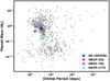Fig. 1

Masses of known transiting exoplanets (gray dots) as a function of their orbital period. The four targets analyzed in this work are shown as colored stars, as in the figure legend. The data were obtained from the NASA Exoplanet Archive (Akeson et al. 2013) on July 30, 2024.

2 Observations

We employed observations from the high-resolution ground-based spectrograph ESPRESSO at the Very Large Telescope (VLT; Pepe et al. 2021) with a spectral resolving power of R ≈ 140 000, and covering the wavelength range 380–788 nm. The data are summarized in Table 1, where we report the observing logs. Further information about discarded datasets that would adversely affect the transmission spectra because of a low signal-to-noise ratio (S/N) or bad weather conditions, for instance, can be found in Sects. 2.1–2.4. The four analyzed targets are shown in Fig. 1. The ESPRESSO Data Reduction Software (DRS) pipeline, as reported in Table 1, was used to reduce all the observations and extract the 1D spectra used for the analysis.

The stellar, planetary, and orbital parameters of the four star-planet systems are shown in Table 2.

2.1 HD 209458b

HD 209458b is a benchmark hot Jupiter orbiting a bright G-type star. This was the first planet found to be transiting its host star (Charbonneau et al. 2000; Henry et al. 2000), and it remains one of the most extensively studied objects in the literature to date. The NaI absorption in transmission spectra was highly debated by comparing observations at high and low resolution with different instruments and telescopes (e.g., Morello et al. 2022).

After the first detection in the early 2000s in low-resolution observations taken with the Space Telescope Imaging Spectrograph (STIS) on board the HST (Charbonneau et al. 2002), upper limits to the Na I absorption were set from the ground a few years later (Snellen 2004; Narita et al. 2005). Numerous other detections were subsequently reported from both ground- and space-based observations (e.g., Sing et al. 2008; Snellen et al. 2008; Albrecht et al. 2009; Langland-Shula et al. 2009; Jensen et al. 2011; Astudillo-Defru & Rojo 2013; Santos et al. 2020), confirming the presence of Na I at both low and high resolution. However, in 2020, the first doubts emerged when Casasayas-Barris et al. (2020) analyzed high-resolution data from the CARMENES and HARPS-N spectrographs and suggested that the spectral features observed in the transmission spectrum of the Na I D lines might be caused by the combined effects of the CLV and RM effect of the star and not by the absorption from the planet. This non-detection was then supported by two nights of high-resolution high-S/N observations with ESPRESSO (Casasayas-Barris et al. 2021; Morello et al. 2022; Dethier & Bourrier 2023). In the analysis of these data, Casasayas-Barris et al. (2021) argued that the spectral features in transmission spectra at 589 nm could be explained by the CLV and RM effects of the star. However, the modeled stellar spectra were unable to perfectly reproduce the observed spectral feature, especially in the transmission LCs of the Na I D lines. The authors indeed emphasize the necessity of using precise stellar models to correctly account for the CLV and RM effect, which might otherwise bias the analysis of transit spectroscopy observations.

We reanalyzed two transits observed with ESPRESSO under the ESO program 1102.C-0744 in July and September 2019. The datasets are the same as were previously analyzed in Casasayas-Barris et al. (2021) (CB21 from hereafter). For this target, all exposures listed in Table 1 were used, and none were discarded.

2.2 WASP-52b

WASP-52b is a highly inflated hot Jupiter around a K-type faint moderately active star (see the S-index in Table 1) with a strong CLV+RM effect (e.g., Chen et al. 2020), and with occulted starspots and faculae observed in transit LCs (e.g., Kirk et al. 2016; Mancini et al. 2017). Na I was detected by Chen et al. (2020) by combining three transits observed at high resolution with ESPRESSO in October and November 2018 under the ESO programs 0102.D-0789 and 0102.C-0493. We reanalyzed these data. From the first two nights, we discarded the last exposure because the S/N was extremely low (S/N < 2).

Several activity indicators were used to monitor WASP-52 during the transit observations, but no excess absorption suggesting activity was registered (see Sect. 5.1 in Chen et al. 2020). Furthermore, Cegla et al. (2023) did not detect any evidence of spot occultations during the same transits in simultaneous photometric observations from the EulerCam (Lendl et al. 2012) and the Next Generation Transit Survey (NGTS; Wheatley et al. 2018).

The atmosphere of WASP-52b is the first atmosphere that was analyzed with the ESPRESSO spectrograph. Na I was previously detected in low-resolution observations from the HST (e.g., Alam et al. 2018) and ground-based telescopes spanning from the optical to the infrared wavelengths (e.g., Chen et al. 2017; Louden et al. 2017; Bruno et al. 2018), as well as with combined data from different instruments (e.g., Bruno et al. 2020). Most of these studies found evidence for a cloudy atmosphere, and specifically, an optically thick and gray cloud layer at high altitudes.

Table 2

Stellar, planetary, and orbital parameters adopted for the four ESPRESSO targets.

2.3 WASP-76b

The exoplanet WASP-76b belongs to the class of ultrahot Jupiters (UHJs), which are highly irradiated gas giants with a surface temperature greater than 2000 K and an atmosphere that is rich in atomic species. It orbits an F-type star with an orbital period of only 1.8 days. Different atmospheric chemistry is expected between the day- and nightside of this type of exoplanet, and asymmetric absorption signatures have indeed been detected during transits of WASP-76b by Ehrenreich et al. (2020). These authors measured a blueshifted Fe I line of about −11.0 ± 0.7 km s⁻¹, which they attributed to a combination of winds and planetary rotation. The data of the two transits observed by ESPRESSO in 2018, which we reanalyze here, were part of the ESO program 1102.C-744. In the analysis, we discarded the last exposure of the second transit because the S/N was very low (S/N ≈ 20). These observations were also analyzed in Tabernero et al. (2021), who reported a strong detection of Na I absorption in the transmission spectra but did not correct for the CLV+RM effect since they estimated the amplitude of the effects to be much smaller than the error bars on the datapoints. NaI was also previously detected in HARPS data (e.g., Seidel et al. 2019; Žák et al. 2019; Langeveld et al. 2022) as a broadened feature of the Na I doublet, but with a lower significance than in the ESPRESSO data. By combining HARPS and ESPRESSO data, Seidel et al. (2021) were able to distinguish between different wind patterns in the lower and upper atmospheres, and they also retrieved the temperature profile of WASP-76b by analyzing the broadened line shape of the Na I doublet. Finally, the same data were analyzed by Kesseli et al. (2022) using the cross-correlation technique, which revealed asymmetries in the radial velocities (RVs) between ingress and egress in most of the detected species, including Na I, and provided insights into the atmospheric dynamics of this planet.

2.4 WASP-127b

WASP-127b is a close-in highly inflated super-Neptune in a misaligned retrograde orbit around a bright slowly rotating G-type star. Low-resolution ground-based observations first revealed a very peculiar atmosphere that is rich in alkali metals (Na I, Li I, and K I), but also shows unexpected signatures of water (Palle et al. 2017; Chen et al. 2018). After this, the presence of Na I was debated in Seidel et al. (2020), who detected the D₂ line, but not the D₁ line in high-resolution HARPS data. However, Na I absorption was again detected at low resolution in a recent analysis of combined HST and Spitzer Space Telescope data (Spake et al. 2021). Moreover, because of its peculiar properties, this exoplanet has been extensively studied since its discovery and was also recently observed by the James Webb Space Telescope (JWST; Barstow et al. 2015) in May and December 2023, under programs GO 2437 and GTO 1201, respectively. ESPRESSO observed two transits of this exoplanet in February and March 2019 under the ESO program 1102.C-0744, and the data were analyzed in Allart et al. (2020). The authors did not correct the transmission spectrum for the CLV+RM effect because the model showed an extremely small amplitude as a result of the unusual planetary orbit. The authors were still able to retrieve a Na I absorption at a confidence level of 9σ that was blueshifted by 2.74 ± 0.79 km s⁻¹. They interpreted this as a signal of the dynamics of the planet atmosphere, specifically, as winds moving from the day- to the nightside. We reanalyzed these ESPRESSO data without discarding any exposure.

3 Synthetic stellar spectra

The synthetic stellar spectra used in the calculations for the CLV+RM model (see Sect. 4.4) were computed with the radiative transfer MPI-parallelized code Balder (Amarsi et al. 2018). The latter originates from the Multi3d code (Botnen & Carlsson 1999; Leenaarts & Carlsson 2009), which is able to solve the restricted NLTE problem for trace elements, for user-specified atomic elements, and for model atmospheres in either 1D or 3D. Balder can also synthesize spectra under the assumption of LTE line formation. The equation of state, the background line opacities, and the continuous opacities were calculated using the BLUE package, as described in Amarsi et al. (2016a,b). Balder solves the radiative transfer equation and the statistical equilibrium equations simultaneously in an iterative way, until convergence of the level populations is reached. When radiative transfer is performed in 3D, the computation is performed along several short characteristic rays at different μ inclinations and azimuthal ϕ angles. We used the following number of rays with the Lobatto quadrature: n_μ = 8 and n_ϕ = 4. The details about the model atmospheres and the model atom used are given in Sects. 3.1 and 3.2, respectively. The computation of the synthetic spectra is described in Sect. 3.3.

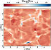Fig. 2

Ratio of the NLTE to LTE equivalent width of Na I 5896 Å for a single STAGGER snapshot of a star with T_eff = 6000 K, log g = 4.5 dex, and [Fe/H]=0.0. In the upflowing granules, overionization weakens the line in NLTE.

3.1 Model atmosphere

Snapshots from 3D radiation-hydrodynamics (RHD) simulations calculated with the STAGGER code (Galsgaard & Nordlund 1995; Stein & Nordlund 1998; Collet et al. 2011; Magic et al. 2013; Collet et al. 2018; Chiavassa et al. 2018; Stein et al. 2024) were employed as model atmospheres for the spectrum synthesis performed in Balder. The detailed 3D NLTE radiative transfer was calculated on five snapshots of each model from the recently updated STAGGER grid (Rodríguez Díaz et al. 2024), adequately spaced so as to capture several convective turnovers. The snapshots were selected according to the procedure described in Sect. 4.4 of Rodríguez Díaz et al. (2024), ensuring that the average hydrodynamic gas properties remained consistent with the full time series. The resulting spectra (intensities at different μ angles) from the five chosen snapshots were then temporally and spatially averaged. We refer to Rodríguez Díaz et al. (2024) for more details about the code and the new STAGGER grid.

The 3D RHD STAGGER model is set on a Cartesian grid of size 240×240×240, corresponding to a physical size that varies from one star to the next, but chosen in such a way as to always include at least ten granules in the simulation. However, in order to decrease the computational time for the spectral synthesis, all the atmospheric snapshots were resized to a resolution of 48×48×240. The vertical dimension is not equidistant in space, but a higher resolution was adopted in the line-forming region (i.e., photosphere). Rodríguez Díaz et al. (2024) showed that reducing the resolution of the horizontal dimension does not significantly affect the resulting spectral line.

Figure 2 displays an example of the spatially resolved 3D NLTE to 3D LTE ratio of the equivalent width (W_λ) of the Na I 5896 Å line at the surface of one of the STAGGER snapshots. NLTE effects strongly depend on the line strength, and since W_λ represents the strength of a spectral line regardless of the spectral resolution, it is a good indicator of discrepancies between LTE and NLTE modeling. The figure shows that the NLTE effects vary over the convection pattern: overpopulation (i.e., W_NLTE/W_LTE > 1) in the intergranular lanes, and under-population in the granules. The steeper temperature gradient of the granules leads to a larger split between the mean radiation field J_ν and the Planck function B_ν, as well as to a more efficient overionization. This effect was observed in the Sun for the Na (Canocchi et al. 2024) as well as for other elements (e.g., Asplund et al. 2004; Lind et al. 2017).

In 3D atmospheres, granulation on the stellar surface arises naturally: The granules are the locations of upflowing hot plasma and gas, whereas the dark intergranular lanes are the locations of downflowing cooler plasma. Analogously, effects such as spectral line broadening and line asymmetries are naturally accounted for in the model itself (e.g., Dravins et al. 1981; Asplund et al. 2000; Dravins et al. 2021) without the need for tunable parameters such as micro- and macroturbulence (v_mic and v_mac), which are typically used in 1D stationary hydrostatic models. For comparison and completeness, we also computed synthetic spectra from 1D MARCS (Gustafsson et al. 2008) model atmospheres and used them throughout this work. We adopted v_mic = 1.0 km s⁻¹ and v_mac = 3.5 km s⁻¹, respectively.

3.2 Model atom

The strong NLTE effects of the Na I atom have been reported in several studies in which NLTE spectra were necessary to reproduce observed data of the Sun and other stars (e.g., Mashonkina et al. 2000; Lind et al. 2011; Asplund et al. 2021; Canocchi et al. 2024). Specifically, the main NLTE effect of the resonance Na I D lines in 1D is that they are affected by over-recombination of the ground state and a subthermal source function, resulting in a stronger line in NLTE than in LTE at the same abundance. For more details about the NLTE effects of Na I, we refer to Sect. 3.1 of Lind et al. (2011) and Sect. 3.2 of Canocchi et al. (2024).

The model atom we used as input for the Balder NLTE calculations was developed and tested in Lind et al. (2011), with modifications as described in Canocchi et al. (2024). It consists of a total of 23 levels: 22 energy levels for Na, and one level for the continuum (Na II). The model includes both radiative and collisional transitions among these energy levels, with detailed quantum mechanical calculations specifically for inelastic collisions involving Na and hydrogen atoms (Belyaev et al. 2010; Barklem et al. 2010) as well as electrons (Park 1971; Allen & Rossouw 1993; Igenbergs et al. 2008). The Na I doublet lines arise from transitions between the 3s–3p_1/2 and 3s–3p_3/2 levels.

3.3 Synthetic spectra

For a given model atom and model atmosphere, radiative transfer calculations were performed independently for three different values of sodium abundances (A(Na)), defined as $A (N a) = \log ϵ_{N a} = \log_{10} (N_{N a} / N_{H}) + 12,$ $\[A(\mathrm{Na})=\log \epsilon_{\mathrm{Na}}=\log _{10}\left(N_{\mathrm{Na}} / N_{\mathrm{H}}\right)+12,\]$ (1)

where N_Na and N_H are the number densities of Na and H. In particular, for each stellar metallicity (i.e., [Fe/H] = log ε_Fe − log ε_{Fe_⊙}), we synthesized spectra for the following sodium abundances: [Na/Fe]³= −0.5, 0.0, and 0.5, that is, within the range of the observed sodium abundance in large spectroscopic stellar surveys such as GALAH (e.g., Amarsi et al. 2020; Buder et al. 2021). The synthetic spectra have a resolving power of R ≈ 500 000 in the Na I D region, covering the wavelength range 5866.0–5920.0 Å. Therefore, a grid of 3D NLTE synthetic spectra was computed for the following stellar parameters: a T_eff between 4500 and 6500 K in steps of 500 K; a log g=4.0, 4.5, and 5.0 dex; and [Fe/H]=−0.5, 0.0, and +0.5 dex. These parameters cover most of the FGK-type stars hosting exoplanets that are observed in transmission spectroscopy studies. Figure 3 shows the Hertzsprung-Russell (HR) diagram with the extent of the computed stellar grid and the locations of the host stars of this work. In addition, the stellar parameters of the synthetic spectra we computed are reported in Table A.3. Seven models are not available in the STAGGER grid: T_eff = 6000 and 6500 K with log g = 5.0 for all three metallicities, and T_eff =5000 K, log g = 4.0, [Fe/H] = −0.5.

We make the grid of synthetic spectra publicly available, together with a Python interpolation routine to obtain the flux and/or intensity spectra at different μ angles for given stellar parameters of T_eff, log g, [Fe/H], and A(Na) (see Sect. 6).

For each of the four targets, we used a simple trilinear interpolation to interpolate the synthetic flux spectra from the grid to the specific T_eff, log g, and [Fe/H] of the host star, using the stellar parameters reported in Table 2. The STAGGER grid, as shown in Fig. 3, is sparse compared to standard 1D grids such as MARCS (Gustafsson et al. 2008), and some of our target stars are located quite far from the grid nodes. In a previous study on a 3D NLTE grid of synthetic spectra for Li I, Wang et al. (2021) investigated the accuracy of different interpolation methods on the STAGGER grid, concluding that the commonly used spline interpolation performs well for spectral line profiles (see Fig. 10 in Wang et al. 2021). However, they suggested that more complex methods, such as those involving neural networks, should be employed for abundance determinations. We decided to use linear interpolation because we found that spline interpolation performs well for relatively weak spectral lines such as the Li I line analyzed by Wang et al. (2021), but it overestimates the flux in the wings of very broad lines such as the Na I D lines. We plan to explore the impact of different and more accurate interpolation methods on our Na I grid in a forthcoming paper, which will also extend the grid of 3D NLTE synthetic spectra to include lower-metallicity models as well as giant stars.

After interpolating the synthetic fluxes from the grid to match the parameters of the four host stars, we normalized the observed out-of-transit fluxes (i.e., the Master Out; see Sect. 4.3) by fitting a first-order polynomial to the local continuum in the region of the Na I D lines and then dividing the data by this polynomial. After this, the synthetic normalized flux of the Na I D lines was fit to the observed normalized Master Out via a standard χ² minimization routine using the Na I abundance (A(Na) (see Table A.3) as a free parameter. Linear interpolation between models was applied. The best-fit value of A(Na), as inferred from the Na I D lines, is reported in Table 2. The resulting best-fit line profile is shown in Fig. 4. The best-fit abundance value was then employed to compute the intensity spectra at the different μ angles used in the analysis of the transmission spectra and LCs to compute the CLV+RM model (see Sect. 4.4).

Similarly, we fit the 3D NLTE synthetic flux to the Na I doublet at 6154 Å and 6160 Å, which is typically used to determine the sodium abundance in metal-rich stars. The synthetic spectra have a resolving power of R ≈ 400 000 in the 6154/6160 Å region, covering the wavelength range 6148–6168 Å. The resulting [Na/F] values are presented in Table 2. These values agree well with those inferred from fitting the NaI D lines, with discrepancies ranging from 0.02 dex for WASP-76b to 0.06 dex for WASP-127b. These discrepancies might be due to unresolved blends, a slightly different continuum placement, or/and various errors in atomic data. We did not compute the CLV+RM model for these lines because they are significantly weaker than the Na I D lines. As a result, the transmission spectra and LCs exhibit variations on the same order of magnitude as the continuum (e.g., 0.05% in HD 209458), which prevents us from detecting any measurable absorption depth in the planet atmosphere using these lines.

The stellar parameters of the four stars were taken from the Gaia DR3 archive (Gaia Collaboration 2023)⁴ and are mostly consistent with other values reported in the literature. We noted a discrepancy between the [Fe/H] values for HD 209458 and WASP-76 from Gaia DR3 and from high-resolution spectroscopic studies in the literature. However, this discrepancy does not significantly affect our results, meaning that the [Fe/H] parameter does not play a critical role in the analysis of the CLV+RM model.

Moreover, we used the 3D NLTE Hα line profiles from the public grid of Amarsi et al. (2018) as a diagnostic to validate the effective temperature. The extremely good agreement of the wings of the Na I D lines with these models is shown in Fig. A.1, where the models are overplotted on the out-of-transit spectra of the four targets.

In Sect. 5 we apply the 3D NLTE synthetic spectra to the high-resolution spectroscopic observations of four bright exoplanet host stars, presented in Sect. 2. We compare them with synthetic spectra computed with Balder in 3D LTE, 1D LTE, and 1D NLTE as well, and we test the improvement, if any, in the (non-)detectability of Na I in their atmospheres.

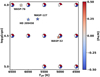Fig. 3

Hertzsprung-Russel diagram illustrating the STAGGER-grid nodes at which the 3D NLTE computations were performed for [Fe/H] = −0.5 (blue), 0.0 (white), and +0.5 (red). Additionally, the four host stars of the gas giants are overplotted, colored by their metallicity.

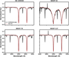Fig. 4

Master Out (in black) around the Na I doublet region. The best-fit synthetic 3D NLTE spectra are overplotted (in red) for HD 209458 (upper left), WASP-52 (upper right), WASP-76 (bottom left), and WASP-127 (bottom right). The two emission spikes in WASP-52 and WASP-127 are due to cosmic rays.

4 Search for Na absorption

The data reduction, including the sky correction, was performed with the ESPRESSO data reduction pipeline, as specified in Table 1. After this, we carried out the following steps for all the targets to search for absorption signatures of Na I in the doublet at 5890 and 5896 Å, which originates from the upper layers of the planetary atmosphere. We extracted the transmission spectrum as presented in previous studies (e.g., Wyttenbach et al. 2015; Casasayas-Barris et al. 2017, 2021; Yan & Henning 2018; Borsa et al. 2021).

4.1 Telluric correction

The telluric emission lines such as those from Na I were removed in the sky-subtraction step. On the other hand, we corrected for telluric absorption lines coming from the Earth’s atmosphere using the ESO software Molecfit (Smette et al. 2015; Kausch et al. 2015) through ExoReflex version 2.11.5. The code produces synthetic spectra of telluric H₂O and O₂ using a line-by-line radiative transfer model of Earth’s atmospheric transmission. The correction was performed in the Earth rest frame and was successfully used in several works that focused on atmospheric composition using the ESPRESSO spectrograph (e.g., Chen et al. 2020; Casasayas-Barris et al. 2021; Borsa et al. 2021).

4.2 Determining the orbital phase

For each night of observations, we calculated the orbital phase of each exposure based on the literature ephemeris (e.g., transit duration, orbital period, and transit epoch), as reported in Table 2. This allowed us to determine the in- and out-of-transit exposures. The latter are defined as the frames with zero overlap with the transit event. The fully in-transit exposures are instead located for more than 50% between the second and third contacts of the transit event. The other exposures are considered either ingress or egress events. Exposures with a low S/N were discarded as described in Sect. 2.

4.3 RV fitting and creation of the Master Out

A linear fit was performed on the radial velocities⁵ (RV) of the out-of-transit frames in order to determine the semi-amplitude of the stellar radial velocity signal (K_⋆; see Table 2). The intransit exposures were discarded for this determination since they contain the RM component.

At this point, all the spectra were shifted to the stellar rest frame (SRF) using the stellar RV-fit model. The systemic velocity (v_sys) was corrected for each night as well.

All the spectra were then normalized using a third-order polynomial function to fit the continuum variations between every individual spectrum. The variations in the Earth’s atmosphere (e.g., airmass) during the night cause the flux to vary between each exposure. Then, the normalized out-of-transit spectra were averaged together to create the Master Out spectrum, using the inverse square of flux uncertainties as the weight. All the not discarded out-of-transit observations, as specified in Sects. 2.1–2.4, were used to generate the Master Out. This resulted in an average relative uncertainty in the final flux ranging from 0.1% for HD 209458 to 0.8% for WASP-52. This procedure was repeated for each night, and the resulting spectra for all the targets are shown in Fig. 4. The best-fit synthetic spectrum produced with 3D NLTE models as described in Sect. 3 is overplotted in this figure.

4.4 Correction for the center-to-limb variation and Rossiter–McLaughlin effect

We modeled the combined effect of the CLV and RM on the Na I D line profiles using the best-fit synthetic stellar spectra as described in Sect. 3. We considered 3D NLTE, 3D LTE, 1D NLTE, and 1D LTE stellar synthetic spectra.

Following the approach of Casasayas-Barris et al. (2019) and Morello et al. (2022), the sky-projected stellar disk was represented as a grid of 300 × 300 squared cells. Each cell had a specific μ angle, radial velocity (v_μ), and intensity spectrum (I_μ) depending on its position on the disk. The intensity spectra were interpolated from the best-fit synthetic spectra at 21 μ angles, ranging from the disk center (μ = 1.0) to near the edge (μ = 0.001), where μ = 0.001 was chosen instead of 0.0 to avoid numerical errors.

The spectra for cells at intermediate μ angles were obtained via linear interpolation. Each cell was associated with Cartesian coordinates (x_i, y_i), assuming a circular stellar disk with a radius R_⋆ = 1, centered on the origin. Therefore, for the ith cell, the μ angle was calculated as $μ_{i} = \sqrt{1 - x_{i}^{2} - y_{i}^{2}}$ $\[\mu_{i}=\sqrt{1-x_{i}^{2}-y_{i}^{2}}\]$ (2)

The local radial velocity (v_i) for each cell was determined by the sky-projected obliquity (λ) and the stellar rotational velocity (v sin i_⋆) using the following equation: $v_{i} = v \sin i_{⋆} (y_{i} \sin λ - x_{i} \cos λ) .$ $\[v_{i}=v \sin i_{\star}\left(y_{i} \sin \lambda-x_{i} \cos \lambda\right).\]$ (3)

The values of λ and v sin i_⋆ for the four targets were taken from the literature and are reported in Table 2. These values can be retrieved by modeling the RM effect on the in-transit spectra, for example, through the reloaded RM technique (Cegla et al. 2016) adopted in CB21 to analyze the HD 209458b data.

In these simulations, we assumed that the star rotates as a solid body, meaning that differential rotation was not considered. At each orbital phase, the stellar spectrum was then obtained by summing the Doppler-shifted spectra from all stellar disk cells that were not obscured by the transiting planet. The resulting CLV+RM models in the transmission spectra using 3D NLTE synthetic spectra around the Na I D lines of each target are shown in Fig. 5. The comparisons between CLV+RM models obtained using different synthetic spectra, that is, 1D LTE, 1D NLTE, 3D LTE, and 3D NLTE, are shown in Figs. 6 and 7, for the Na I D₁ and D₂, respectively. Finally, we show in Figs. A.3 and A.4 the CLV+RM models for the transmission LCs.

4.5 Creating the transmission spectrum

To obtain the transmission spectrum of each exposure in the stellar rest frame, each in-transit spectrum in the SRF (F_i,in) was divided by the Master Out. As the planet moves across the stellar disk during a transit, it gradually blocks the light from regions with varying velocities and CLV. In the case of an aligned orbit, the planet initially covers the blueshifted side of the star at ingress, followed by the redshifted side near egress. This causes distortions in the spectral line profiles due to the stellar rotation. This phenomenon is referred to as the Doppler shadow (Collier Cameron et al. 2010). The latter is clearly visible in the two-dimensional map in Fig. 8, where the ratio of the in- to out-of-transit flux observed for each phase of HD 209458b is displayed, together with the corresponding CLV+RM model from the 3D NLTE synthetic spectra.

All the residual spectra were then shifted to the planet rest frame (PRF) by computing the planet velocity at each phase ϕ through the following equation: $v_{p} = K_{p} \sin (2 π ϕ),$ $\[v_{\mathrm{p}}=K_{\mathrm{p}} \sin (2 \pi \phi),\]$ (4)

where K_p is the planet RV semi-amplitude obtained from transit parameters such as the semi-major axis a, the orbital inclination i_p, and the orbital period P_orb as follows, assuming zero eccentricity: $K_{p} = \frac{2 π a}{P_{orb}} \sin (i_{p}) .$ $\[K_{\mathrm{p}}=\frac{2 \pi a}{P_{\text {orb }}} \sin \left(i_{\mathrm{p}}\right).\]$ (5)

The K_p calculated with this equation for each target is reported in Table 2. Finally, to compute the transmission spectrum, all the in-transit residuals were combined with an arithmetic average.

For better visualization of the resulting transmission spectra, they were binned in wavelength to either 0.05 Å (for HD 209458b) or 0.10 Å (for WASP-52b, WASP-76b, and WASP-127b). This is shown in Fig. 5.

An issue with ESPRESSO data that has been highlighted in several previous studies (e.g., Casasayas-Barris et al. 2021; Tabernero et al. 2021) is the interference sinusoidal pattern, the wiggles that arise when spectra taken at different times during the same night are divided, that is, in transmission spectra. These wiggles are due to non-flat-fielded interference that occurs in some optical elements of the Coude’ train. The ESPRESSO wiggles were corrected for by fitting a third-order spline to the combined transmission spectrum of each night, as previously performed by Jiang et al. (2023). An example of this correction is shown in Fig. A.2.

After the wiggle-pattern correction, the CLV+RM model was subtracted from the data as well in order to obtain the final transmission spectrum. Transmission spectra from different transits were coadded using a weighted average. Finally, a Gaussian fit was performed on the absorption features (if any) corresponding to the Na I D lines. The corrected transmission spectra are shown in Fig. 9. The absorption depth inferred from the Gaussian fit is reported in Table 3, and is compared there with measurements from previous works that used the same datasets. Other properties of the line fit (i.e., FWHM and Doppler shift) are reported in Table A.1.

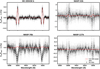Fig. 5

Wiggle-corrected transmission spectra (in black) of the Na I D lines. The CLV+RM model from 3D NLTE stellar spectra (in red) is overplotted for HD 209458 (upper left), WASP-52 (upper right), WASP-76 (bottom left), and WASP-127 (bottom right).

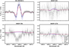Fig. 6

Same as Fig. 5, but zoomed-in on the Na I D₁ line. The CLV+RM model from different synthetic stellar spectra is overplotted: 3D NLTE (solid blue line), 3D LTE (solid red line), 1D NLTE (dashed blue line), and 1D LTE (dashed red line).

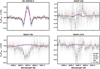Fig. 7

Same as Fig. 5, but zoomed-in on the Na I D₂ line. The CLV+RM model from different synthetic stellar spectra is overplotted: 3D NLTE (solid blue line), 3D LTE (solid red line), 1D NLTE (dashed blue line), and 1D LTE (dashed red line).

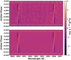Fig. 8

Two-dimensional map of HD 209458 during a transit by its planet (first night), in the stellar rest frame. Top: in- to out-of-transit flux observed by ESPRESSO on 2019 July 20. Bottom: in- to out-of-transit flux produced with the best-fit 3D NLTE synthetic spectra. The dashed white lines represent the beginning and end of the transit.

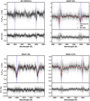Fig. 9

Transmission spectra corrected for the CLV+RM effect using 3D NLTE models around the Na I D lines. The gray dots represent the original data, and the black dots are the binned data (with a binning of 0.05 Å for HD 209458b and 0.1 Å for the others). Top: best Gaussian fit to the data overplotted (solid red line). The rest-frame wavelength of each individual line is represented by a dashed vertical blue line. The scales of the y-axis are different. Bottom: residuals between the data and the Gaussian fit.

4.6 Creating the transmission light curve

As done in previous studies of the Na I D lines (e.g., Yan et al. 2017; Casasayas-Barris et al. 2020, 2021), considering the transmission spectra in the PRF, the transmission LCs were obtained by fixing a passband of a given width Δλ = 0.75 Å or 0.4 Å around the center of the line that was to be analyzed, and we then calculated the flux inside the passband using trapezoidal integration. In order to perform this calculation, we used tools from ExoTETHys⁶ (Morello et al. 2020a,b, 2021), following the procedure detailed in Morello et al. (2022). As in CB21, the LCs of different nights were combined by sorting the values measured at different time stamps in chronological order with respect to the center of the transit. In this way, an interpolation to a common time axis can be avoided. For visualization purposes, the combined data were then binned to 0.001 in orbital phase. The transmission LCs of the average of the two Na I D lines of HD 209458b are displayed in Fig. 10, and they are shown for the other targets in Figs. A.3 and A.4 for the 0.75 Å and 0.4 Å passband, respectively.

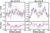Fig. 10

Transmission LCs of HD 209458b in comparison with models of the CLV+RM effect from synthetic stellar spectra, colored as in the figure legend. Left: transmission LC computed in a passband of 0.75 Å around the Na I D lines, averaged together, and binned to 0.001 in orbital phases for better visualization. Right: transmission LC in a passband of 0.4 Å. In the bottom panels, we show the difference between the binned data and the models.

Table 3

Measured depths of the Gaussian fits to the Na I D lines in the transmission spectra for all targets after correcting for the CLV+RM effect with 3D NLTE models.

5 Results

We applied the different synthetic models described in Sect. 3 to correct for the stellar spectrum effect (CLV+RM model) imprinted on ESPRESSO transmission data of four giant exoplanets orbiting relatively bright host stars. We compare the four stellar models computed with different assumptions, that is, 1D LTE, 1D NLTE, 3D LTE, and 3D NLTE, to the transmission spectrum of the targets in Sect. 5.1. The transmission light curve of HD 209458b is also analyzed in Sect. 5.2.

Moreover, we discuss the CLV effects over the grid of 3D NLTE synthetic stellar spectra in Sect. 5.3. We also simulate the variation in the CLV+RM effect of the HD 209458 system within the parameter space of the stellar grid in Sect. 5.4.

5.1 Transmission spectra

As already shown in several works (e.g., Czesla et al. 2015; Casasayas-Barris et al. 2020), depending on the geometry of the star-planet system, the amplitude of the CLV+RM effect can be as strong as the absorption feature itself. One of the main parameters affecting the shape of the CLV+RM effect is λ, the sky-projected angle. For aligned orbits, such as those of HD 209458b and WASP-52b (see Table 2), the amplitude of the stellar CLV on the planetary transmission spectrum and LCs can be as large as 0.5% (e.g., Yan et al. 2017). This is indeed the case for systems HD 209458 and the WASP-52. Specifically, for HD 209458b, the difference between the adopted stellar model is significant, and a large scatter up to ± 0.2% for the 1 D models was indeed observed when the residuals between the data and the models were computed: +0.2% for the 1D NLTE, and about −0.2% for the 1D LTE. This is illustrated in Fig. 11, where the transmission spectrum is zoomed-in on the Na I D₁ line to visualize the differences between the synthetic spectra better. Different stellar models result in varying amplitudes of the line deformations. Figure 11 clearly shows that only the 3D NLTE model results in an extremely good fit of the observed transmission spectrum of the Na I D₁ line. On the other hand, the 1D LTE and NLTE models result in an underestimate and overestimate, respectively, of the observed amplitude in the line core. The same behavior is observed for the Na I D₂ line, as shown in the top left panel of Fig. 7. Specifically, the residuals obtained with the 1D NLTE model show a dip in the line core that can be mistaken for a Na absorption feature corresponding to an absorption depth of about 0.2% when this stellar model is adopted. Then, if a 3D stellar atmosphere is used in the LTE assumption, the resulting CLV+RM model produces a curve with the smallest amplitude (of 0.23% at maximum) among all the other stellar models, which translates into a peak in the line core of about +0.2% in the corresponding residuals. With the 3D NLTE models, the CLV+RM curve instead shows a peak at about 0.4% at the line center and a minimum of about −0.25% in the line wings. This matches the data perfectly. Therefore, we obtain essentially flat residuals when we subtract the 3D NLTE model from the data. This indicates that no additional Na absorption is required to explain the behavior of the Na I D lines in the transmission spectrum of HD 209458b and supports the results of CB21, namely that no Na is detected in the atmosphere of this planet at the layers probed by high-resolution spectroscopy. However, this result does not necessarily contradict the many Na detections at low resolution. Indeed, Na could still be present in small quantities, colder than equilibrium temperature and/or deeper atmospheric layers without significantly affecting the transmission spectrum at high resolution, as shown by Morello et al. (2022).

For the other planets, namely the WASP systems, the average S/N is lower and the error bars on the data points are slightly larger than in HD 209458b, which makes it more challenging to distinguish between various stellar models. Despite these challenges, differences remain between the models, although the detection and measurement of Na absorption can be achieved even without correcting for the CLV+RM effect, albeit with a reduced confidence level. After correcting for the CLV+RM effect using a 3D NLTE model, we measured an absorption depth that was consistent with previous literature studies that either did not apply this correction or used a 1D model. The results are summarized in Table 3.

For WASP-52b, the amplitude of the 3D NLTE curve is the largest of the models. It reaches a peak of about 0.2% at the line center. The differences with the other stellar models are smaller than 0.1%, as shown in Figs. 6 and 7. Because the error bars on the binned data range between 0.13% and 0.47%, it is not possible to distinguish the results of the different models (see Table A.2). The planetary absorption obtained after correcting for the CLV+RM effect with the 3D NLTE model is shown in the top right panel of Fig. 9, where the Na features were fit with Gaussians. The absorption depths measured after correcting for the CLV+RM effect with 3D NLTE models are larger than those measured by Chen et al. (2020), who used 1D LTE SME models. Specifically, the absorption depth of the Na I D₁ is larger by about 14%, whereas the D₂ line depth increases by about 33%, as reported in Table 3. Without the CLV+RM correction, we measure smaller absorption depths, even closer to the results of Chen et al. (2020). Our results are generally consistent with theirs, except for the Doppler shift in wavelength. While they did not observe this shift, our Gaussian fits indicate a blueshift that corresponds to a wind velocity of approximately −8.0 km s⁻¹. Additionally, no broadening in the absorption line wings is observed.

With the continuous improvements of high-resolution spectrographs, higher S/N will likely be achieved in the near future, resulting in lower error bars similar to those for HD 209458b. Consequently, it will be crucial to adopt the most accurate stellar model for the correct characterization of exoplanetary atmospheres.

For WASP-76b, the error bars on the binned data are on the same order of magnitude as those of HD 209458b. They range between 0.04% and 0.08%. However, due to the significantly misaligned orbit (λ = 61.28 deg), the amplitude of the CLV+RM effect becomes quite small. Specifically, it reaches a maximum of 0.03% for the 3D NLTE model and 0.06% for the 1D LTE model, which exhibits the largest amplitude in this instance. Moreover, in this case, the Na absorption is so evident in the transmission spectrum that it can be detected even without correcting for the CLV+RM effect (see Fig. 5), which should not make a significant difference given its amplitude. However, after correcting the transmission spectra for the CLV+RM effect with the 3D NLTE model and fitting the Na I D lines, we found a Na absorption depth that exceeded the values reported by Tabernero et al. (2021) by about 14% and 22% for the D₁ and D₂ lines, respectively (see Table 3). Furthermore, we were able to retrieve the Na absorption with a higher confidence level, that is, 18σ instead of the 9.2σ of Tabernero et al. (2021). Therefore, we conclude that given the WASP-76b absorption depth is about 0.4% (much smaller than in the WASP-52b case), the correction for the CLV+RM effect does indeed make a difference by improving the detection confidence level, even though the amplitude of the effect is extremely small. Moreover, the absorption features we observe are slightly broadened and blueshifted by about −4.3 ± 0.5 km s⁻¹, indicating the presence of winds in the planet atmosphere. This is consistent with the results of Tabernero et al. (2021).

For WASP-127b, a system with a highly misaligned and retrograde orbit (i.e., λ = −128.41 deg), all the CLV+RM models result in an essentially flat curve with a maximum amplitude of about 0.03%, except for the 1D LTE model, which reaches a peak of 0.05%. However, given the spread of the data points and because the error bars are on the same order of magnitude as the CLV+RM effect, namely within 0.04–0.13%, correcting for this effect does not appear to be important in this system. After correcting for the CLV+RM effect with the 3D NLTE model, we retrieved an absorption depth, averaged between the two Na I D lines, of 0.35 ± 0.04%, which agrees perfectly with the value measured by Allart et al. (2020), who did not perform any correction. We also observed an average Doppler shift of −3.2 ± 0.4 km s⁻¹, indicating the presence of winds in the planetary atmosphere, as previously reported by Allart et al. (2020). In line with their results, we also found a significant asymmetry between the absorption depths of the Na I D lines, with a line ratio of D₂/D₁ = 2.4. Previous studies investigated possible explanations for a D₂/D₁ line ratio that differed from unity and suggested a variety of scenarios that ranged from stellar activity to variability in the chemical composition or in velocity distribution of the Na I atoms, as well as whether the absorption occurs in an optically thin or thick regime (Gebek & Oza 2020).

Our results suggest that for an extremely misaligned orbit such as that in the WASP-127 system, there is no need for correcting for the CLV+RM effect because it does not significantly affect the detection and measurement of Na I absorption, if present.

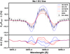Fig. 11

Transmission spectrum of HD 209458b centered on the Na I D₁ line, compared with models of the CLV+RM effect from synthetic stellar spectra, colored as in the figure legend. We show in the bottom panel the difference between the binned data and the models.

5.2 Transmission light curves

As previously observed in other studies, the shape of the transmission LCs varies depending on the selected bandwidth: narrower bandwidths result in stronger LC amplitudes (e.g., Yan et al. 2017; Canocchi et al. 2024). Therefore, we selected the narrow bandwidths of 0.75 Å and 0.4 Å to maximize the LC amplitude so that we could compare it to our models.

The transmission LCs in bandwidths of 0.75 Å and 0.4 Å for HD 209458b are shown in Fig. 10 in the left and right panels, respectively. In both cases, the 1D NLTE model overestimates the amplitude at mid-transit.

In the 0.75 Å LC, it is difficult to distinguish the best model because all models are within the error bars of the data points, except for the 1D NLTE model, which clearly overestimates the data in the mid-transit part. On the other hand, in the case of 0.4 Å, the LTE models, both 1D and 3D, underestimate the ingress and egress parts of the transit. A better match is obtained from the 3D NLTE model, but it is still not perfect in the mid-transit part because it does not reach far enough. To completely rule out the presence of Na I, we would expect the CLV+RM model to perfectly fit the observed data, as shown in the transmission spectrum (see Sect. 5.1).

Because this is not the case, our results suggest that the 3D NLTE models perform better than the others, in particular, they outperform the commonly used 1D models. Further improvement can be achieved, however. For instance, recent studies have shown that magnetic fields impact the limb darkening and the observed CLV in solar-type stars (e.g., Ludwig et al. 2023; Kostogryz et al. 2024). Magnetic fields indeed modify the stellar atmospheric structure, which in turn affects the CLV of spectral lines. As shown in Figs. 2 and 3 in Ludwig et al. (2023), both the averaged temperature profile and the spatial-temporal temperature fluctuation vary with magnetic field strength. Specifically, the 3D radiation-magnetohydrodynamic (RMHD) model atmospheres computed by Ludwig et al. (2023) were able to reduce but not completely eliminate the small systematic discrepancy between observations and models of the CLV. Further work is required to investigate the role of stellar magnetic activity in transmission spectra and LCs of exoplanets. Further advancements in 3D NLTE synthetic spectra could be achieved from improvements to the model atmosphere, for example, in terms of opacity binning or resolution, or from improvements to the model atom, such as more accurate collisional rates, or from lifting the trace-element assumption.

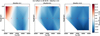Fig. 12

CLV effect across the STAGGER grid for FGK-type stars. The panels show the ratio of the combined equivalent width of the Na I D lines from 3D NLTE synthetic spectra at the limb (μ = 0.1) and at the disk center (μ = 1.0). The red dots indicate the grid nodes at which the synthetic spectra were computed.

5.3 CLV effects in the stellar grid

The intrinsic variations of the stellar lines from the disk center to the limb are determined by the stellar parameters. The stellar effective temperature has the strongest impact on the CLV effect (Yan et al. 2015, 2017). The widths of the Na I D lines, indeed, increase as T_eff decreases. Line broadening in the wings occurs primarily because the ground state of Na I is increasingly populated at low temperatures (i.e., the line opacity increases) (Lind et al. 2011). The CLV and T_eff dependence of the Na I D lines is well illustrated in Fig. 3 in Czesla et al. (2015).

In order to investigate the CLV effect across the stellar grid (Fig. 3) as a function of the stellar parameters of T_eff, log g, and [Fe/H], we computed the combined equivalent width (W_λ) of the Na I D lines at different μ angles by integrating the 3D NLTE synthetic spectra in the wavelength range 5866.0–5920.0 Å, that is, the range of our synthetic spectra in the region of the Na I D lines. We did not compute the W_λ of the Na I D₁ and D₂ separately because in models with low T_eff (i.e., 4500 K), the wings of the two lines become extremely broadened, causing them to blend. We show the ratio of W_λ at the limb (μ = 0.1) to that at the disk center (μ = 1.0) in Fig. 12, with contour plots that illustrate the variation in this ratio with effective temperature and surface gravity at a sodium abundance of [Na/Fe] = 0.

The relative difference between the line strength at the limb and at the disk center shows significant variations across the stellar grid of 3D NLTE spectra, ranging between about ±20%. The strongest positive variations, meaning a stronger line at the limb, occur at high temperatures (i.e., T_eff = 6500 K) and low surface gravities (i.e., log g = 4.0 dex), where the line contrast reaches up to 28% for [Fe/H]=−0.5. Conversely, the lines become weaker at the limb in the rest of the grid, particularly in metal-rich stars (i.e., [Fe/H]=+0.5) with low T_eff. For instance, at T_eff = 5000 K and log g = 5.0 dex, the difference decreases by as much as −21%. This could be explained as a line-strength effect: the cooler the star, the stronger the lines, and the more they are weakened at the limb compared to disk center.

In 1D LTE (see Fig. A.5) the lines are always weaker at the limb across the entire grid, with variations ranging from about −38% to −46% for lower metallicity. In 3D NLTE instead (see Fig. 12), for high T_eff, the lines at the limb become stronger than at the disk center, especially for low metallicity (i.e., [Fe/H]=−0.5). This occurs due to the velocity fields that naturally arise in the 3D model atmosphere, which are absent in the 1D model. This effect can be reproduced in 1D by using a depth-dependent v_mic (Takeda 2022), for instance.

In addition to the CLV effect, we also observed that the difference in equivalent width between 3D and 1D models is as significant as the CLV effect itself across the entire grid. A more detailed discussion of this effect will be provided in a forthcoming paper, which will extend the grid to include lower-metallicity models and giants.

Moreover, Fig. 13 shows the CLV of the Na I D lines in the four host stars, that is, their W_λ as a function of μ angles. These were obtained from the best-fit synthetic spectra in 1D LTE, 1D NLTE, 3D LTE, and 3D NLTE (see Sect. 3). It is evident that the 1D LTE model dramatically exaggerates the CLV effect compared to the 3D NLTE model. The 1D models underestimate the equivalent width more toward the limb due to the lack of velocity fields, as previously shown by Reiners et al. (2023). The LTE underestimation toward the limb suggests increased photon losses in shallower layers, as observed by Canocchi et al. (2024).

5.4 CLV+RM effects in the stellar grid

This section illustrates how the CLV+RM model for the HD 209458b planetary system would change if the planet were orbiting different types of FGK-type stars. Considering the planetary and orbital parameters of this system (see Table 2), we computed the CLV+RM model for the transmission LC in a 0.75 Å passband using 3D NLTE synthetic spectra from the stellar grid with a solar sodium abundance, that is, [Na/Fe] = 0.

A contour diagram of the mid-transit values for the CLV+RM curves in the 0.75 Å passband is shown in Fig. 14. We chose to plot the mid-transit value of the LC because it appears to be the datapoint with the strongest variation among models (e.g., see Fig. 10). The contour diagrams show that the amplitude of the CLV+RM curve increases with lower T_eff and higher log g. The overall variations are within 0.26%. This result agrees with the findings of Yan et al. (2017), according to whom stars with lower T_eff exhibit a stronger CLV+RM effect. Nevertheless, the shape of the CLV + RM in transmission spectra and LCs is determined by orbital and planetary parameters, and it might be important to correct for it also for stars with high T_eff, as demonstrated in the case of HD 209458b. Figure 14 shows that this planet lies in a part of the grid that is minimally affected by the CLV+RM effect, yet our analysis shows that accounting for it is essential when transmission spectra and LCs have to be interpreted. If HD 209458b were orbiting a cooler star, the CLV+RM effect would be even more pronounced, making the correction even more critical.

Moreover, in addition to the host star, several orbital parameters play a crucial role in shaping the CLV+RM model in transmission spectra and LCs. They include in particular the impact parameter (b), the planet-to-star radius ratio (R_p/R_⋆), and the sky-projected obliquity (λ). Specifically, the impact parameter, which is related to the orbit inclination, and R_p/R_⋆ affect the amplitude of the curve (e.g., Canocchi et al. 2024). The actual shape is instead determined by λ, which describes the transit trajectory on the stellar disk.

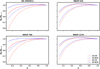Fig. 13

Center-to-limb variation of the equivalent width (W_λ) of the combined Na I D lines for the best-fit synthetic spectra of the four targets, colored as in the figure legend.

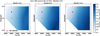Fig. 14

Contour diagram of the mid-transit value of the CLV+RM model of the transmission light curve in a 0.75 Å band for a planet with the same planetary and orbital properties as HD 209458b, but orbiting FGK-type stars from the STAGGER grid. The red dots indicate the grid nodes at which the synthetic spectra were computed. The red star indicates the location of the true HD 209458 star in the grid.

6 Conclusions

We modeled the CLV of the strong Na I D lines at 5890 Å and 5896 Å of the host stars of four giant planets using 3D RHD stellar models and NLTE line formation. We applied the synthetic spectra to compute the CLV+RM effect on the transmission spectra as well as the LCs of the four targets. We then corrected the data taken with the high-resolution ESPRESSO spectrograph at the VLT during different campaigns for this effect. We also made a comparison with other synthetic spectra, and specifically, with the commonly used 1D LTE models computed with the MARCS (Gustafsson et al. 2008) grid, as well as models in 1D NLTE and 3D LTE. For the 3D simulations, we used five statistically independent snapshots for each model from the recently extended and refined STAGGER grid, published in Rodríguez Díaz et al. (2024).

Our work supports the previous detections of NaI in the WASP systems. It improves the accuracy of the measurements and makes the detections more statistically significant, except for systems in highly misaligned orbits such as WASP-127b. We also confirmed the findings of CB21, namely that there is no detection of Na I in the atmosphere of HD 209458b at the layers probed by high-resolution spectroscopy. The CLV+RM model computed using 3D NLTE synthetic spectra perfectly matches the observed transmission spectrum of the Na I D lines, and it also is in good agreement with the transmission LCs.

For some configurations of the planet-star system, the CLV+RM effects do not significantly affect the resulting transmission spectra, as in the case of WASP-127b, which is in an extremely misaligned orbit. However, for some other planets, such as HD 209458b, the CLV+RM effect can be as strong as the planetary atmospheric feature, and depending on the orbital geometry, it can even overlap the expected planetary atmosphere tracks (e.g., Czesla et al. 2015). For these planets, with the transmission spectra now achieving high-quality data due to advanced spectrographs such as ESPRESSO, the CLV+RM effect is thus within the S/N of these observations and can no longer be disregarded. We conclude that 3D NLTE synthetic spectra can be used to improve the accuracy of the analyses of transmission data of exoplanet atmospheres from current and future ground-based high-resolution spectrographs, such as the forthcoming ANDES on the Extremely Large Telescope (ELT; Palle et al. 2023). The correction of the CLV+RM effect will become even more crucial when colder planets are studied, such as super-Earths, where the planetary atmosphere track will overlap these stellar effects even more. For this purpose, we publish a grid of 3D NLTE synthetic spectra for Na I, for FGK-type stars with the following stellar parameters:

An effective temperature (T_eff) between 4500 and 6500 K in steps of 500 K.
A surface gravity (log g) between 4.0 and 5.0 in steps of 0.5.
A metallicity ([Fe/H]) between −0.5 and +0.5 in steps of 0.5.
A sodium abundance ([Na/Fe]) between −0.5 and +0.5 in steps of 0.5.

Together with the grid, we publish a Python interpolation routine that allows the computation of intensity spectra for any given stellar parameters and for any given μ angles. In this way, the method presented in this work can easily be extended to other FGK host-stars in order to compute a more accurate CLV+RM effect of the NaI D lines for any planet-star system.

An accurate analysis of the transmission spectra in the optical wavelength region from ground-based facilities is fundamental to complement the high-quality space-based observations in the infrared from telescopes such as the current JWST (Gardner et al. 2006; Barstow et al. 2015), and in the future, from ARIEL (Tinetti et al. 2016, 2018).

Even though we did not detect any Na I absorption in HD 209458b from our high-resolution transmission spectra, absorption from this species can still be observed at low and medium resolution. This has recently been shown by Carteret et al. (2024), who investigated the impact of the RM effect on space-based data of HD 209458b. Their findings suggest that the observed absorption feature could be explained by absorption in the wings of the Na I D lines, and not from the core probed at high resolution. They also found that absorption signatures from Na I at medium resolution with instruments such as JWST/NIRSPEC or HST/STIS can be significantly biased by the RM effect if this is not properly accounted for. Therefore, an important issue to address in the near future would be to evaluate the impact of 3D NLTE synthetic stellar spectra on these types of datasets as well.

Finally, several other spectral lines relevant to transmission spectroscopy have been shown to be significantly affected by strong 3D NLTE effects (e.g., the Hα line, Amarsi et al. 2018; the K I resonance line, Canocchi et al. 2024). Future work includes the study and investigation of the impact of 3D NLTE models on other atomic species detected in exoplanet atmospheres, such as Ca I, Ca II (e.g., Yan et al. 2019), Fe I (e.g., Hoeijmakers et al. 2018), Fe II (e.g., Bello-Arufe et al. 2022), the Hi Balmer lines (e.g., Fossati et al. 2023), and the Mg I triplet (e.g., Hoeijmakers et al. 2020; Prinoth et al. 2024). We refer to Lind & Amarsi (2024) for a review of 3D NLTE stellar models.

In a forthcoming paper, we will extend the grid of 3D NLTE spectra for Na I to FGK-giants (i.e., log g = 1.5–3.5) and metalpoor stars with a metallicity down to [Fe/H]=−4 in order to explore the impact of the 3D model atmosphere on the stellar sodium abundance determination.

Data availability

The grid of 3D NLTE synthetic spectra for FGK-type dwarfs is only available in electronic form at https://doi.org/10.5281/zenodo.13881827.

Acknowledgements

We thank the anonymous referee for their comments, which have improved the quality of the manuscript. GC and KL acknowledge funds from the Knut and Alice Wallenberg foundation. KL also acknowledges funds from the European Research Council (ERC) under the European Union’s Horizon 2020 research and innovation programme (Grant agreement No. 852977). GM acknowledges financial support from the Severo Ochoa grant CEX2021-001131-S and from the Ramón y Cajal grant RYC2022-037854-I funded by MCIN/AEI/10.13039/501100011033 and FSE+. We thank the PDC Center for High Performance Computing, KTH Royal Institute of Technology, Sweden, for providing access to computational resources and support. The computations were enabled by resources provided by the National Academic Infrastructure for Supercomputing in Sweden (NAISS), partially funded by the Swedish Research Council through grant agreement no. 2022-06725, at the PDC Center for High Performance Computing, KTH Royal Institute of Technology (project numbers NAISS 2023/1-15 and NAISS 2024/1-14). This research has made use of NASA’s Astrophysics Data System (ADS) bibliographic services. We acknowledge financial support from the Agencia Estatal de Investigación of the Ministerio de Ciencia e Innovación MCIN/AEI/10.13039/501100011033 and the ERDF “A way of making Europe” through project PID2021-125627OB-C32, and from the Centre of Excellence “Severo Ochoa” award to the Instituto de Astrofisica de Canarias. We acknowledge the community efforts devoted to the development of the following open-source packages that were used in this work: numpy (https://numpy.org), matplotlib (https://matplotlib.org) and astropy (https://astropy.org).

Appendix A Additional tables and figures

The wind velocity in the three WASP planets is computed as the Doppler shift of the line centroids from the Gaussian fit (λ_fit) with respect to the rest frame wavelength (λ₀), as follows: $v_{w i n d} = c \frac{λ_{f i t} - λ_{0}}{λ_{0}},$ $\[v_{{wind }}=c \frac{\lambda_{{fit }}-\lambda_{0}}{\lambda_{0}},\]$ (A.1)

with λ₀ being the rest frame wavelength of the Na I D lines. We first compute v_wind separately for the Na I D₁ and D₂, and then we take the weighted average of the two values, as reported in Table A.1. The Table presents the values from the best-fit Gaussians after correcting for the CLV+RM effect using 3D NLTE stellar models.

Table A.1

Wind velocities, standard deviation (σ), and full width at half maximum (FWHM) of the Gaussian fits for the three gas giants analyzed in this work where Na I was detected.

Table A.2

Measured depths (%) of the Gaussian fits to the Na I D lines in the transmission spectra for the four targets analyzed in this work, after correcting for the CLV + RM effect with different stellar models (1D LTE, 1D NLTE, 3D LTE, and 3D NLTE).

In Table A.2, the absorption depths of the Na I D₁ and D₂ lines, corrected for the CLV+RM effect using different stellar models, are shown.

It is interesting to note that for HD 209458b, all models except the 3D NLTE model detect Na I with a significance level larger than 5σ. The only non-detection occurs when using the 3D NLTE stellar spectra.

For WASP-52b, a system with an aligned orbit, the 3D NLTE model results in a detection with a slightly higher confidence level compared to other models, although the measured depths are consistent within their uncertainties.

In the cases of the heavily misaligned systems WASP-76b and WASP-127b, the use of a 3D NLTE model does not significantly enhance the detection’s significance. The measured absorption depths from various models agree well within their uncertainties.

Table A.3

Parameters of the 3D NLTE synthetic spectra computed in the grid for this work.

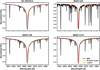Fig. A.1

Master Out around the Hα line profiles observed with ESPRESSO in the four target stars, compared to the 3D NLTE model with T_eff, log g, [Fe/H], and v sin i_⋆ listed in Table 2. The orange shaded region indicates the effect of adjusting the T_eff by ± 100 K.

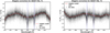Fig. A.2

Transmission spectra (in black) of WASP-76b with overplotted the wiggles model, that is a third-order spline (in red). Left: In- to out-of-transit flux observed by ESPRESSO on 2018-09-03. Right: In- to out-of-transit flux observed by ESPRESSO on 2018-10-31.

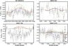Fig. A.3

Transmission LCs in a 0.75 Å passband centered on the Na I D lines. The gray dots represent the original data, whereas the black dots are the data binned to 0.001 in orbital phase. The CLV+RM model from different synthetic stellar spectra is overplotted, colored as in the figure’s legend. It is worth noticing the different scale of the y-axis.

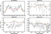Fig. A.4

Transmission LCs in a 0.4 Å passband centered on the Na I D lines. The gray dots represent the original data, whereas the black dots are the data binned to 0.001 in orbital phase. The CLV+RM model from different synthetic stellar spectra is overplotted, colored as in the figure’s legend. It is worth noticing the different scale of the y-axis.

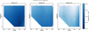Fig. A.5

The CLV effect across the stellar grid for FGK-type stars. The panels show the ratio of the combined equivalent width of the Na I D lines from 1D LTE synthetic spectra at the limb (μ = 0.1) and at the disk center (μ = 1.0). The red dots indicate the grid nodes where the synthetic spectra have been computed.

References

Akeson, R. L., Chen, X., Ciardi, D., et al. 2013, PASP, 125, 989 [Google Scholar]
Alam, M. K., Nikolov, N., López-Morales, M., et al. 2018, AJ, 156, 298 [NASA ADS] [CrossRef] [Google Scholar]
Albrecht, S., Snellen, I., de Mooij, E., & Le Poole, R. 2009, in Transiting Planets, 253, eds. F. Pont, D. Sasselov, & M. J. Holman, 520 [Google Scholar]
Allart, R., Pino, L., Lovis, C., et al. 2020, A&A, 644, A155 [NASA ADS] [CrossRef] [EDP Sciences] [Google Scholar]
Allen, L. J., & Rossouw, C. J. 1993, Phys. Rev. B, 47, 2446 [NASA ADS] [CrossRef] [Google Scholar]
Amarsi, A. M., Asplund, M., Collet, R., & Leenaarts, J. 2016a, MNRAS, 455, 3735 [NASA ADS] [CrossRef] [Google Scholar]
Amarsi, A. M., Lind, K., Asplund, M., Barklem, P. S., & Collet, R. 2016b, MNRAS, 463, 1518 [NASA ADS] [CrossRef] [Google Scholar]
Amarsi, A. M., Nordlander, T., Barklem, P. S., et al. 2018, A&A, 615, A139 [NASA ADS] [CrossRef] [EDP Sciences] [Google Scholar]
Amarsi, A. M., Nissen, P. E., Asplund, M., Lind, K., & Barklem, P. S. 2019, A&A, 622, L4 [NASA ADS] [CrossRef] [EDP Sciences] [Google Scholar]
Amarsi, A. M., Lind, K., Osorio, Y., et al. 2020, A&A, 642, A62 [EDP Sciences] [Google Scholar]
Asplund, M., Nordlund, Å., Trampedach, R., Allende Prieto, C., & Stein, R. F. 2000, A&A, 359, 729 [Google Scholar]
Asplund, M., Grevesse, N., Sauval, A. J., Allende Prieto, C., & Kiselman, D. 2004, A&A, 417, 751 [NASA ADS] [CrossRef] [EDP Sciences] [Google Scholar]
Asplund, M., Amarsi, A. M., & Grevesse, N. 2021, A&A, 653, A141 [NASA ADS] [CrossRef] [EDP Sciences] [Google Scholar]
Astudillo-Defru, N., & Rojo, P. 2013, A&A, 557, A56 [NASA ADS] [CrossRef] [EDP Sciences] [Google Scholar]
Barklem, P. S., Belyaev, A. K., Dickinson, A. S., & Gadéa, F. X. 2010, A&A, 519, A20 [NASA ADS] [CrossRef] [EDP Sciences] [Google Scholar]
Barstow, J. K., Aigrain, S., Irwin, P. G. J., Kendrew, S., & Fletcher, L. N. 2015, MNRAS, 448, 2546 [NASA ADS] [CrossRef] [Google Scholar]
Bello-Arufe, A., Buchhave, L. A., Mendonça, J. M., et al. 2022, A&A, 662, A51 [NASA ADS] [CrossRef] [EDP Sciences] [Google Scholar]
Belyaev, A. K., Barklem, P. S., Dickinson, A. S., & Gadéa, F. X. 2010, Phys. Rev. A, 81, 032706 [NASA ADS] [CrossRef] [Google Scholar]
Bergemann, M., Hoppe, R., Semenova, E., et al. 2021, MNRAS, 508, 2236 [NASA ADS] [CrossRef] [Google Scholar]
Bjørgen, J. P., Sukhorukov, A. V., Leenaarts, J., et al. 2018, A&A, 611, A62 [Google Scholar]
Borsa, F., & Zannoni, A. 2018, A&A, 617, A134 [NASA ADS] [CrossRef] [EDP Sciences] [Google Scholar]
Borsa, F., Allart, R., Casasayas-Barris, N., et al. 2021, A&A, 645, A24 [EDP Sciences] [Google Scholar]
Botnen, A., & Carlsson, M. 1999, in Astrophysics and Space Science Library, 240, Numerical Astrophysics, eds. S. M. Miyama, K. Tomisaka, & T. Hanawa, 379 [NASA ADS] [CrossRef] [Google Scholar]
Brown, T. M. 2001, ApJ, 553, 1006 [NASA ADS] [CrossRef] [Google Scholar]
Bruno, G., Lewis, N. K., Stevenson, K. B., et al. 2018, AJ, 156, 124 [NASA ADS] [CrossRef] [Google Scholar]
Bruno, G., Lewis, N. K., Alam, M. K., et al. 2020, MNRAS, 491, 5361 [NASA ADS] [Google Scholar]
Buder, S., Sharma, S., Kos, J., et al. 2021, MNRAS, 506, 150 [NASA ADS] [CrossRef] [Google Scholar]
Canocchi, G., Lind, K., Lagae, C., et al. 2024, A&A, 683, A242 [NASA ADS] [CrossRef] [EDP Sciences] [Google Scholar]
Carteret, Y., Bourrier, V., & Dethier, W. 2024, A&A, 683, A63 [NASA ADS] [CrossRef] [EDP Sciences] [Google Scholar]
Casasayas-Barris, N., Palle, E., Nowak, G., et al. 2017, A&A, 608, A135 [NASA ADS] [CrossRef] [EDP Sciences] [Google Scholar]
Casasayas-Barris, N., Pallé, E., Yan, F., et al. 2019, A&A, 628, A9 [NASA ADS] [CrossRef] [EDP Sciences] [Google Scholar]
Casasayas-Barris, N., Pallé, E., Yan, F., et al. 2020, A&A, 635, A206 [NASA ADS] [CrossRef] [EDP Sciences] [Google Scholar]
Casasayas-Barris, N., Palle, E., Stangret, M., et al. 2021, A&A, 647, A26 [NASA ADS] [CrossRef] [EDP Sciences] [Google Scholar]
Cegla, H. M., Lovis, C., Bourrier, V., et al. 2016, A&A, 588, A127 [NASA ADS] [CrossRef] [EDP Sciences] [Google Scholar]
Cegla, H. M., Roguet-Kern, N., Lendl, M., et al. 2023, A&A, 674, A174 [NASA ADS] [CrossRef] [EDP Sciences] [Google Scholar]
Charbonneau, D., Brown, T. M., Latham, D. W., & Mayor, M. 2000, ApJ, 529, L45 [Google Scholar]
Charbonneau, D., Brown, T. M., Noyes, R. W., & Gilliland, R. L. 2002, ApJ, 568 377 [Google Scholar]
Chen, G., Pallé, E., Nortmann, L., et al. 2017, A&A, 600, L11 [NASA ADS] [CrossRef] [EDP Sciences] [Google Scholar]
Chen, G., Pallé, E., Welbanks, L., et al. 2018, A&A, 616, A145 [NASA ADS] [CrossRef] [EDP Sciences] [Google Scholar]
Chen, G., Casasayas-Barris, N., Pallé, E., et al. 2020, A&A, 635, A171 [NASA ADS] [CrossRef] [EDP Sciences] [Google Scholar]
Chiavassa, A., & Brogi, M. 2019, A&A, 631, A100 [NASA ADS] [CrossRef] [EDP Sciences] [Google Scholar]
Chiavassa, A., Casagrande, L., Collet, R., et al. 2018, A&A, 611, A11 [NASA ADS] [CrossRef] [EDP Sciences] [Google Scholar]
Collet, R., Magic, Z., & Asplund, M. 2011, in Journal of Physics Conference Series, 328, 012003 [NASA ADS] [CrossRef] [Google Scholar]
Collet, R., Nordlund, Å., Asplund, M., Hayek, W., & Trampedach, R. 2018, MNRAS, 475, 3369 [NASA ADS] [CrossRef] [Google Scholar]
Collier Cameron, A., Bruce, V. A., Miller, G. R. M., Triaud, A. H. M. J., & Queloz, D. 2010, MNRAS, 403, 151 [NASA ADS] [CrossRef] [Google Scholar]
Cosentino, R., Lovis, C., Pepe, F., et al. 2012, SPIE Conf. Ser., 8446, 84461V [Google Scholar]
Czesla, S., Klocová, T., Khalafinejad, S., Wolter, U., & Schmitt, J. H. M. M. 2015, A&A, 582, A51 [NASA ADS] [CrossRef] [EDP Sciences] [Google Scholar]
Dethier, W., & Bourrier, V. 2023, A&A, 674, A86 [NASA ADS] [CrossRef] [EDP Sciences] [Google Scholar]
Dravins, D., Lindegren, L., & Nordlund, A. 1981, A&A, 96, 345 [NASA ADS] [Google Scholar]
Dravins, D., Ludwig, H.-G., & Freytag, B. 2021, A&A, 649, A16 [NASA ADS] [CrossRef] [EDP Sciences] [Google Scholar]
Ehrenreich, D., Lovis, C., Allart, R., et al. 2020, Nature, 580, 597 [Google Scholar]
Ellwarth, M., Schäfer, S., Reiners, A., & Zechmeister, M. 2023, A&A, 673, A19 [NASA ADS] [CrossRef] [EDP Sciences] [Google Scholar]
Evans, T. M., Aigrain, S., Gibson, N., et al. 2015, MNRAS, 451, 680 [Google Scholar]
Fossati, L., Biassoni, F., Cappello, G. M., et al. 2023, A&A, 676, A99 [NASA ADS] [CrossRef] [EDP Sciences] [Google Scholar]
Fu, G., Deming, D., Lothringer, J., et al. 2021, AJ, 162, 108 [NASA ADS] [CrossRef] [Google Scholar]
Gaia Collaboration (Vallenari, A., et al.) 2023, A&A, 674, A1 [NASA ADS] [CrossRef] [EDP Sciences] [Google Scholar]
Galsgaard, K., & Nordlund, A. 1995, A 3D MHD Code for Parallel Computers [Google Scholar]
Gardner, J. P., Mather, J. C., Clampin, M., et al. 2006, Space Sci. Rev., 123, 485 [Google Scholar]
Gebek, A., & Oza, A. V. 2020, MNRAS, 497, 5271 [Google Scholar]
Gomes da Silva, J., Figueira, P., Santos, N., & Faria, J. 2018, J. Open Source Softw., 3, 667 [Google Scholar]
Gomes da Silva, J., Santos, N. C., Adibekyan, V., et al. 2021, A&A, 646, A77 [NASA ADS] [CrossRef] [EDP Sciences] [Google Scholar]
Gustafsson, B., Edvardsson, B., Eriksson, K., et al. 2008, A&A, 486, 951 [NASA ADS] [CrossRef] [EDP Sciences] [Google Scholar]
Hébrard, G., Collier Cameron, A., Brown, D. J. A., et al. 2013, A&A, 549, A134 [NASA ADS] [CrossRef] [EDP Sciences] [Google Scholar]
Henry, G. W., Marcy, G. W., Butler, R. P., & Vogt, S. S. 2000, ApJ, 529, L41 [Google Scholar]
Hoeijmakers, H. J., Ehrenreich, D., Heng, K., et al. 2018, Nature, 560, 453 [CrossRef] [Google Scholar]
Hoeijmakers, H. J., Seidel, J. V., Pino, L., et al. 2020, A&A, 641, A123 [NASA ADS] [CrossRef] [EDP Sciences] [Google Scholar]
Igenbergs, K., Schweinzer, J., Bray, I., Bridi, D., & Aumayr, F. 2008, At. Data Nucl. Data Tables, 94, 981 [NASA ADS] [CrossRef] [Google Scholar]
Jensen, A. G., Redfield, S., Endl, M., et al. 2011, ApJ, 743, 203 [Google Scholar]
Jiang, Z., Wang, W., Chen, G., et al. 2023, A&A, 677, A110 [NASA ADS] [CrossRef] [EDP Sciences] [Google Scholar]
Kausch, W., Noll, S., Smette, A., et al. 2015, A&A, 576, A78 [NASA ADS] [CrossRef] [EDP Sciences] [Google Scholar]
Kesseli, A. Y., Snellen, I. A. G., Casasayas-Barris, N., Mollière, P., & SánchezLópez, A. 2022, AJ, 163, 107 [NASA ADS] [CrossRef] [Google Scholar]
Kirk, J., Wheatley, P. J., Louden, T., et al. 2016, MNRAS, 463, 2922 [NASA ADS] [CrossRef] [Google Scholar]
Knutson, H. A., Charbonneau, D., Noyes, R. W., Brown, T. M., & Gilliland, R. L. 2007, ApJ, 655, 564 [NASA ADS] [CrossRef] [Google Scholar]
Kostogryz, N. M., Shapiro, A. I., Witzke, V., et al. 2024, arXiv e-prints [arXiv:2403.00118] [Google Scholar]
Lam, K. W. F., Faedi, F., Brown, D. J. A., et al. 2017, A&A, 599, A3 [NASA ADS] [CrossRef] [EDP Sciences] [Google Scholar]
Langeveld, A. B., Madhusudhan, N., & Cabot, S. H. C. 2022, MNRAS, 514, 5192 [NASA ADS] [CrossRef] [Google Scholar]
Langland-Shula, L. E., Vogt, S. S., Charbonneau, D., Butler, P., & Marcy, G. 2009, ApJ, 696, 1355 [NASA ADS] [CrossRef] [Google Scholar]
Leenaarts, J., & Carlsson, M. 2009, in Astronomical Society of the Pacific Conference Series, 415, The Second Hinode Science Meeting: Beyond DiscoveryToward Understanding, eds. B. Lites, M. Cheung, T. Magara, J. Mariska, & K. Reeves, 87 [Google Scholar]
Lendl, M., Anderson, D. R., Collier-Cameron, A., et al. 2012, A&A, 544, A72 [NASA ADS] [CrossRef] [EDP Sciences] [Google Scholar]
Lind, K., & Amarsi, A. M. 2024, ARA&A, 62, 475 [NASA ADS] [CrossRef] [Google Scholar]
Lind, K. & Amarsi, A. M. 2024, Annual Review of Astronomy and Astrophysics L [Google Scholar]
Lind, K., Asplund, M., Barklem, P. S., & Belyaev, A. K. 2011, A&A, 528, A103 [NASA ADS] [CrossRef] [EDP Sciences] [Google Scholar]
Lind, K., Amarsi, A. M., Asplund, M., et al. 2017, MNRAS, 468, 4311 [NASA ADS] [CrossRef] [Google Scholar]
Louden, T., Wheatley, P. J., Irwin, P. G. J., Kirk, J., & Skillen, I. 2017, MNRAS, 470, 742 [NASA ADS] [CrossRef] [Google Scholar]
Ludwig, H. G., Steffen, M., & Freytag, B. 2023, A&A, 679, A65 [NASA ADS] [CrossRef] [EDP Sciences] [Google Scholar]
Madhusudhan, N., Knutson, H., Fortney, J. J., & Barman, T. 2014, in Protostars and Planets VI, eds. H. Beuther, R. S. Klessen, C. P. Dullemond, & T. Henning, 739 [Google Scholar]
Magic, Z., Collet, R., Asplund, M., et al. 2013, A&A, 557, A26 [NASA ADS] [CrossRef] [EDP Sciences] [Google Scholar]
Mancini, L., Southworth, J., Raia, G., et al. 2017, MNRAS, 465, 843 [NASA ADS] [CrossRef] [Google Scholar]
Mashonkina, L. I., Shimanskii, V. V., & Sakhibullin, N. A. 2000, Astron. Rep., 44, 790 [NASA ADS] [CrossRef] [Google Scholar]
Mayor, M., Pepe, F., Queloz, D., et al. 2003, The Messenger, 114, 20 [NASA ADS] [Google Scholar]
McLaughlin, D. B. 1924, ApJ, 60, 22 [Google Scholar]
Mordasini, C., van Boekel, R., Mollière, P., Henning, T., & Benneke, B. 2016, ApJ, 832, 41 [Google Scholar]
Morello, G., Claret, A., Martin-Lagarde, M., et al. 2020a, J. Open Source Softw., 5, 1834 [CrossRef] [Google Scholar]
Morello, G., Claret, A., Martin-Lagarde, M., et al. 2020b, AJ, 159, 75 [NASA ADS] [CrossRef] [Google Scholar]
Morello, G., Zingales, T., Martin-Lagarde, M., Gastaud, R., & Lagage, P.-O. 2021, AJ, 161, 174 [NASA ADS] [CrossRef] [Google Scholar]
Morello, G., Casasayas-Barris, N., Orell-Miquel, J., et al. 2022, A&A, 657, A97 [NASA ADS] [CrossRef] [EDP Sciences] [Google Scholar]
Naef, D., Mayor, M., Beuzit, J. L., et al. 2004, A&A, 414, 351 [NASA ADS] [CrossRef] [EDP Sciences] [Google Scholar]
Narita, N., Suto, Y., Winn, J. N., et al. 2005, PASJ, 57, 471 [NASA ADS] [Google Scholar]
Nordlander, T., & Lind, K. 2017, A&A, 607, A75 [NASA ADS] [CrossRef] [EDP Sciences] [Google Scholar]
Öberg, K. I., Murray-Clay, R., & Bergin, E. A. 2011, ApJ, 743, L16 [Google Scholar]
Palle, E., Chen, G., Prieto-Arranz, J., et al. 2017, A&A, 602, L15 [NASA ADS] [CrossRef] [EDP Sciences] [Google Scholar]
Palle, E., Biazzo, K., Bolmont, E., et al. 2023, arXiv e-prints [arXiv:2311.17075] [Google Scholar]
Park, C. 1971, J. Quant. Spec. Radiat. Transf., 11, 7 [NASA ADS] [CrossRef] [Google Scholar]
Pepe, F. A., Cristiani, S., Rebolo Lopez, R., et al. 2010, SPIE Conf. Ser., 7735, 77350F [Google Scholar]
Pepe, F., Molaro, P., Cristiani, S., et al. 2014, Astron. Nachr., 335, 8 [Google Scholar]
Pepe, F., Cristiani, S., Rebolo, R., et al. 2021, A&A, 645, A96 [NASA ADS] [CrossRef] [EDP Sciences] [Google Scholar]
Pereira, T. M. D., Asplund, M., Collet, R., et al. 2013, A&A, 554, A118 [NASA ADS] [CrossRef] [EDP Sciences] [Google Scholar]
Pietrow, A. G. M., Cretignier, M., Druett, M. K., et al. 2024, A&A, 682, A46 [NASA ADS] [CrossRef] [EDP Sciences] [Google Scholar]
Pietrow, A. G. M., & Pastor Yabar, A. 2023, arXiv e-prints [arXiv:2311.06200] [Google Scholar]
Piskunov, N., & Valenti, J. A. 2017, A&A, 597, A16 [NASA ADS] [CrossRef] [EDP Sciences] [Google Scholar]
Prinoth, B., Hoeijmakers, H. J., Morris, B. M., et al. 2024, A&A, 685, A60 [NASA ADS] [CrossRef] [EDP Sciences] [Google Scholar]
Redfield, S., Endl, M., Cochran, W. D., & Koesterke, L. 2008, ApJ, 673, L87 [Google Scholar]
Reiners, A., Yan, F., Ellwarth, M., Ludwig, H. G., & Nortmann, L. 2023, A&A, 673, A71 [NASA ADS] [CrossRef] [EDP Sciences] [Google Scholar]
Richardson, L. J., Harrington, J., Seager, S., & Deming, D. 2006, ApJ, 649, 1043 [NASA ADS] [CrossRef] [Google Scholar]
Rodríguez Díaz, L. F., Lagae, C., Amarsi, A. M., et al. 2024, A&A, 688, A212 [NASA ADS] [CrossRef] [EDP Sciences] [Google Scholar]
Rossiter, R. A. 1924, ApJ, 60, 15 [Google Scholar]
Rutten, R. J. 2003, Radiative Transfer in Stellar Atmospheres [Google Scholar]
Santos, N. C., Cristo, E., Demangeon, O., et al. 2020, A&A, 644, A51 [NASA ADS] [CrossRef] [EDP Sciences] [Google Scholar]
Scharmer, G. B., Bjelksjo, K., Korhonen, T. K., Lindberg, B., & Petterson, B. 2003, SPIE Conf. Ser., 4853, 341 [NASA ADS] [Google Scholar]
Seidel, J. V., Ehrenreich, D., Wyttenbach, A., et al. 2019, A&A, 623, A166 [NASA ADS] [CrossRef] [EDP Sciences] [Google Scholar]
Seidel, J. V., Lendl, M., Bourrier, V., et al. 2020, A&A, 643, A45 [NASA ADS] [CrossRef] [EDP Sciences] [Google Scholar]
Seidel, J. V., Ehrenreich, D., Allart, R., et al. 2021, A&A, 653, A73 [NASA ADS] [CrossRef] [EDP Sciences] [Google Scholar]
Sing, D. K., Vidal-Madjar, A., Désert, J. M., Lecavelier des Etangs, A., & Ballester, G. 2008, ApJ, 686, 658 [Google Scholar]
Smette, A., Sana, H., Noll, S., et al. 2015, A&A, 576, A77 [NASA ADS] [CrossRef] [EDP Sciences] [Google Scholar]
Snellen, I. A. G. 2004, MNRAS, 353, L1 [Google Scholar]
Snellen, I. A. G., Albrecht, S., de Mooij, E. J. W., & Le Poole, R. S. 2008, A&A, 487, 357 [NASA ADS] [CrossRef] [EDP Sciences] [Google Scholar]
Spake, J. J., Sing, D. K., Wakeford, H. R., et al. 2021, MNRAS, 500, 4042 [Google Scholar]
Stein, R. F., & Nordlund, Å. 1998, ApJ, 499, 914 [Google Scholar]
Stein, R. F., Nordlund, Å., Collet, R., & Trampedach, R. 2024, ApJ, 970, 24 [NASA ADS] [CrossRef] [Google Scholar]
Tabernero, H. M., Zapatero Osorio, M. R., Allart, R., et al. 2021, A&A, 646, A158 [NASA ADS] [CrossRef] [EDP Sciences] [Google Scholar]
Takeda, Y. 2022, Sol. Phys., 297, 4 [NASA ADS] [CrossRef] [Google Scholar]
Tinetti, G., Drossart, P., Eccleston, P., et al. 2016, SPIE Conf. Ser., 9904, 99041X [NASA ADS] [Google Scholar]
Tinetti, G., Drossart, P., Eccleston, P., et al. 2018, Exp. Astron., 46, 135 [NASA ADS] [CrossRef] [Google Scholar]
Torres, G., Winn, J. N., & Holman, M. J. 2008, ApJ, 677, 1324 [Google Scholar]
Valenti, J. A., & Piskunov, N. 1996, A&AS, 118, 595 [NASA ADS] [CrossRef] [EDP Sciences] [Google Scholar]
Wang, E. X., Nordlander, T., Asplund, M., et al. 2021, MNRAS, 500, 2159 [Google Scholar]
Wheatley, P. J., West, R. G., Goad, M. R., et al. 2018, MNRAS, 475, 4476 [Google Scholar]
Wyttenbach, A., Ehrenreich, D., Lovis, C., Udry, S., & Pepe, F. 2015, A&A, 577, A62 [NASA ADS] [CrossRef] [EDP Sciences] [Google Scholar]
Yan, F., & Henning, T. 2018, Nat. Astron., 2, 714 [Google Scholar]
Yan, F., Fosbury, R. A. E., Petr-Gotzens, M. G., Zhao, G., & Pallé, E. 2015, A&A, 574, A94 [NASA ADS] [CrossRef] [EDP Sciences] [Google Scholar]
Yan, F., Pallé, E., Fosbury, R. A. E., Petr-Gotzens, M. G., & Henning, T. 2017, A&A, 603, A73 [NASA ADS] [CrossRef] [EDP Sciences] [Google Scholar]
Yan, F., Casasayas-Barris, N., Molaverdikhani, K., et al. 2019, A&A, 632, A69 [NASA ADS] [CrossRef] [EDP Sciences] [Google Scholar]
Žák, J., Kabáth, P., Boffin, H. M. J., Ivanov, V. D., & Skarka, M. 2019, AJ, 158, 120 [Google Scholar]

¹

https://research.iac.es/proyecto/exoatmospheres/index.php

²

μ = cos θ, with θ defined as the angle between the outward normal of the stellar surface and the observer’s line of sight.

³

[Na/Fe]=[Na/H]-[Fe/H].

⁴

https://gea.esac.esa.int/archive/

⁵

The RV measurements are given as output of the ESPRESSO data reduction pipeline.

⁶

https://github.com/ucl-exoplanets/exotethys

All Tables

Table 1

Observing log for the ESPRESSO observations.

In the text

Table 2

Stellar, planetary, and orbital parameters adopted for the four ESPRESSO targets.

In the text

Table 3

Measured depths of the Gaussian fits to the Na I D lines in the transmission spectra for all targets after correcting for the CLV+RM effect with 3D NLTE models.

In the text

Table A.1

Wind velocities, standard deviation (σ), and full width at half maximum (FWHM) of the Gaussian fits for the three gas giants analyzed in this work where Na I was detected.

In the text

Table A.2

Measured depths (%) of the Gaussian fits to the Na I D lines in the transmission spectra for the four targets analyzed in this work, after correcting for the CLV + RM effect with different stellar models (1D LTE, 1D NLTE, 3D LTE, and 3D NLTE).

In the text

Table A.3

Parameters of the 3D NLTE synthetic spectra computed in the grid for this work.

In the text

All Figures

	Fig. 1 Masses of known transiting exoplanets (gray dots) as a function of their orbital period. The four targets analyzed in this work are shown as colored stars, as in the figure legend. The data were obtained from the NASA Exoplanet Archive (Akeson et al. 2013) on July 30, 2024.
In the text

	Fig. 2 Ratio of the NLTE to LTE equivalent width of Na I 5896 Å for a single STAGGER snapshot of a star with T_eff = 6000 K, log g = 4.5 dex, and [Fe/H]=0.0. In the upflowing granules, overionization weakens the line in NLTE.
In the text

	Fig. 3 Hertzsprung-Russel diagram illustrating the STAGGER-grid nodes at which the 3D NLTE computations were performed for [Fe/H] = −0.5 (blue), 0.0 (white), and +0.5 (red). Additionally, the four host stars of the gas giants are overplotted, colored by their metallicity.
In the text

	Fig. 4 Master Out (in black) around the Na I doublet region. The best-fit synthetic 3D NLTE spectra are overplotted (in red) for HD 209458 (upper left), WASP-52 (upper right), WASP-76 (bottom left), and WASP-127 (bottom right). The two emission spikes in WASP-52 and WASP-127 are due to cosmic rays.
In the text

	Fig. 5 Wiggle-corrected transmission spectra (in black) of the Na I D lines. The CLV+RM model from 3D NLTE stellar spectra (in red) is overplotted for HD 209458 (upper left), WASP-52 (upper right), WASP-76 (bottom left), and WASP-127 (bottom right).
In the text

	Fig. 6 Same as Fig. 5, but zoomed-in on the Na I D₁ line. The CLV+RM model from different synthetic stellar spectra is overplotted: 3D NLTE (solid blue line), 3D LTE (solid red line), 1D NLTE (dashed blue line), and 1D LTE (dashed red line).
In the text

	Fig. 7 Same as Fig. 5, but zoomed-in on the Na I D₂ line. The CLV+RM model from different synthetic stellar spectra is overplotted: 3D NLTE (solid blue line), 3D LTE (solid red line), 1D NLTE (dashed blue line), and 1D LTE (dashed red line).
In the text

	Fig. 8 Two-dimensional map of HD 209458 during a transit by its planet (first night), in the stellar rest frame. Top: in- to out-of-transit flux observed by ESPRESSO on 2019 July 20. Bottom: in- to out-of-transit flux produced with the best-fit 3D NLTE synthetic spectra. The dashed white lines represent the beginning and end of the transit.
In the text

Fig. 9

Transmission spectra corrected for the CLV+RM effect using 3D NLTE models around the Na I D lines. The gray dots represent the original data, and the black dots are the binned data (with a binning of 0.05 Å for HD 209458b and 0.1 Å for the others). Top: best Gaussian fit to the data overplotted (solid red line). The rest-frame wavelength of each individual line is represented by a dashed vertical blue line. The scales of the y-axis are different. Bottom: residuals between the data and the Gaussian fit.

In the text

Fig. 10

Transmission LCs of HD 209458b in comparison with models of the CLV+RM effect from synthetic stellar spectra, colored as in the figure legend. Left: transmission LC computed in a passband of 0.75 Å around the Na I D lines, averaged together, and binned to 0.001 in orbital phases for better visualization. Right: transmission LC in a passband of 0.4 Å. In the bottom panels, we show the difference between the binned data and the models.

In the text

	Fig. 11 Transmission spectrum of HD 209458b centered on the Na I D₁ line, compared with models of the CLV+RM effect from synthetic stellar spectra, colored as in the figure legend. We show in the bottom panel the difference between the binned data and the models.
In the text

	Fig. 12 CLV effect across the STAGGER grid for FGK-type stars. The panels show the ratio of the combined equivalent width of the Na I D lines from 3D NLTE synthetic spectra at the limb (μ = 0.1) and at the disk center (μ = 1.0). The red dots indicate the grid nodes at which the synthetic spectra were computed.
In the text

	Fig. 13 Center-to-limb variation of the equivalent width (W_λ) of the combined Na I D lines for the best-fit synthetic spectra of the four targets, colored as in the figure legend.
In the text

Fig. 14

Contour diagram of the mid-transit value of the CLV+RM model of the transmission light curve in a 0.75 Å band for a planet with the same planetary and orbital properties as HD 209458b, but orbiting FGK-type stars from the STAGGER grid. The red dots indicate the grid nodes at which the synthetic spectra were computed. The red star indicates the location of the true HD 209458 star in the grid.

In the text

	Fig. A.1 Master Out around the Hα line profiles observed with ESPRESSO in the four target stars, compared to the 3D NLTE model with T_eff, log g, [Fe/H], and v sin i_⋆ listed in Table 2. The orange shaded region indicates the effect of adjusting the T_eff by ± 100 K.
In the text

	Fig. A.2 Transmission spectra (in black) of WASP-76b with overplotted the wiggles model, that is a third-order spline (in red). Left: In- to out-of-transit flux observed by ESPRESSO on 2018-09-03. Right: In- to out-of-transit flux observed by ESPRESSO on 2018-10-31.
In the text

	Fig. A.3 Transmission LCs in a 0.75 Å passband centered on the Na I D lines. The gray dots represent the original data, whereas the black dots are the data binned to 0.001 in orbital phase. The CLV+RM model from different synthetic stellar spectra is overplotted, colored as in the figure’s legend. It is worth noticing the different scale of the y-axis.
In the text

	Fig. A.4 Transmission LCs in a 0.4 Å passband centered on the Na I D lines. The gray dots represent the original data, whereas the black dots are the data binned to 0.001 in orbital phase. The CLV+RM model from different synthetic stellar spectra is overplotted, colored as in the figure’s legend. It is worth noticing the different scale of the y-axis.
In the text

	Fig. A.5 The CLV effect across the stellar grid for FGK-type stars. The panels show the ratio of the combined equivalent width of the Na I D lines from 1D LTE synthetic spectra at the limb (μ = 0.1) and at the disk center (μ = 1.0). The red dots indicate the grid nodes where the synthetic spectra have been computed.
In the text

Current usage metrics show cumulative count of Article Views (full-text article views including HTML views, PDF and ePub downloads, according to the available data) and Abstracts Views on Vision4Press platform.

Data correspond to usage on the plateform after 2015. The current usage metrics is available 48-96 hours after online publication and is updated daily on week days.

Initial download of the metrics may take a while.

[1] Akeson, R. L., Chen, X., Ciardi, D., et al. 2013, PASP, 125, 989 [Google Scholar]

[2] Alam, M. K., Nikolov, N., López-Morales, M., et al. 2018, AJ, 156, 298 [NASA ADS] [CrossRef] [Google Scholar]

[3] Albrecht, S., Snellen, I., de Mooij, E., & Le Poole, R. 2009, in Transiting Planets, 253, eds. F. Pont, D. Sasselov, & M. J. Holman, 520 [Google Scholar]

[4] Allart, R., Pino, L., Lovis, C., et al. 2020, A&A, 644, A155 [NASA ADS] [CrossRef] [EDP Sciences] [Google Scholar]

[5] Allen, L. J., & Rossouw, C. J. 1993, Phys. Rev. B, 47, 2446 [NASA ADS] [CrossRef] [Google Scholar]

[6] Amarsi, A. M., Asplund, M., Collet, R., & Leenaarts, J. 2016a, MNRAS, 455, 3735 [NASA ADS] [CrossRef] [Google Scholar]

[7] Amarsi, A. M., Lind, K., Asplund, M., Barklem, P. S., & Collet, R. 2016b, MNRAS, 463, 1518 [NASA ADS] [CrossRef] [Google Scholar]

[8] Amarsi, A. M., Nordlander, T., Barklem, P. S., et al. 2018, A&A, 615, A139 [NASA ADS] [CrossRef] [EDP Sciences] [Google Scholar]

[9] Amarsi, A. M., Nissen, P. E., Asplund, M., Lind, K., & Barklem, P. S. 2019, A&A, 622, L4 [NASA ADS] [CrossRef] [EDP Sciences] [Google Scholar]

[10] Amarsi, A. M., Lind, K., Osorio, Y., et al. 2020, A&A, 642, A62 [EDP Sciences] [Google Scholar]

[11] Asplund, M., Nordlund, Å., Trampedach, R., Allende Prieto, C., & Stein, R. F. 2000, A&A, 359, 729 [Google Scholar]

[12] Asplund, M., Grevesse, N., Sauval, A. J., Allende Prieto, C., & Kiselman, D. 2004, A&A, 417, 751 [NASA ADS] [CrossRef] [EDP Sciences] [Google Scholar]

[13] Asplund, M., Amarsi, A. M., & Grevesse, N. 2021, A&A, 653, A141 [NASA ADS] [CrossRef] [EDP Sciences] [Google Scholar]

[14] Astudillo-Defru, N., & Rojo, P. 2013, A&A, 557, A56 [NASA ADS] [CrossRef] [EDP Sciences] [Google Scholar]

[15] Barklem, P. S., Belyaev, A. K., Dickinson, A. S., & Gadéa, F. X. 2010, A&A, 519, A20 [NASA ADS] [CrossRef] [EDP Sciences] [Google Scholar]

[16] Barstow, J. K., Aigrain, S., Irwin, P. G. J., Kendrew, S., & Fletcher, L. N. 2015, MNRAS, 448, 2546 [NASA ADS] [CrossRef] [Google Scholar]

[17] Bello-Arufe, A., Buchhave, L. A., Mendonça, J. M., et al. 2022, A&A, 662, A51 [NASA ADS] [CrossRef] [EDP Sciences] [Google Scholar]

[18] Belyaev, A. K., Barklem, P. S., Dickinson, A. S., & Gadéa, F. X. 2010, Phys. Rev. A, 81, 032706 [NASA ADS] [CrossRef] [Google Scholar]

[19] Bergemann, M., Hoppe, R., Semenova, E., et al. 2021, MNRAS, 508, 2236 [NASA ADS] [CrossRef] [Google Scholar]

[20] Bjørgen, J. P., Sukhorukov, A. V., Leenaarts, J., et al. 2018, A&A, 611, A62 [Google Scholar]

[21] Borsa, F., & Zannoni, A. 2018, A&A, 617, A134 [NASA ADS] [CrossRef] [EDP Sciences] [Google Scholar]

[22] Borsa, F., Allart, R., Casasayas-Barris, N., et al. 2021, A&A, 645, A24 [EDP Sciences] [Google Scholar]

[23] Botnen, A., & Carlsson, M. 1999, in Astrophysics and Space Science Library, 240, Numerical Astrophysics, eds. S. M. Miyama, K. Tomisaka, & T. Hanawa, 379 [NASA ADS] [CrossRef] [Google Scholar]

[24] Brown, T. M. 2001, ApJ, 553, 1006 [NASA ADS] [CrossRef] [Google Scholar]

[25] Bruno, G., Lewis, N. K., Stevenson, K. B., et al. 2018, AJ, 156, 124 [NASA ADS] [CrossRef] [Google Scholar]

[26] Bruno, G., Lewis, N. K., Alam, M. K., et al. 2020, MNRAS, 491, 5361 [NASA ADS] [Google Scholar]

[27] Buder, S., Sharma, S., Kos, J., et al. 2021, MNRAS, 506, 150 [NASA ADS] [CrossRef] [Google Scholar]

[28] Canocchi, G., Lind, K., Lagae, C., et al. 2024, A&A, 683, A242 [NASA ADS] [CrossRef] [EDP Sciences] [Google Scholar]

[29] Carteret, Y., Bourrier, V., & Dethier, W. 2024, A&A, 683, A63 [NASA ADS] [CrossRef] [EDP Sciences] [Google Scholar]

[30] Casasayas-Barris, N., Palle, E., Nowak, G., et al. 2017, A&A, 608, A135 [NASA ADS] [CrossRef] [EDP Sciences] [Google Scholar]

[31] Casasayas-Barris, N., Pallé, E., Yan, F., et al. 2019, A&A, 628, A9 [NASA ADS] [CrossRef] [EDP Sciences] [Google Scholar]

[32] Casasayas-Barris, N., Pallé, E., Yan, F., et al. 2020, A&A, 635, A206 [NASA ADS] [CrossRef] [EDP Sciences] [Google Scholar]

[33] Casasayas-Barris, N., Palle, E., Stangret, M., et al. 2021, A&A, 647, A26 [NASA ADS] [CrossRef] [EDP Sciences] [Google Scholar]

[34] Cegla, H. M., Lovis, C., Bourrier, V., et al. 2016, A&A, 588, A127 [NASA ADS] [CrossRef] [EDP Sciences] [Google Scholar]

[35] Cegla, H. M., Roguet-Kern, N., Lendl, M., et al. 2023, A&A, 674, A174 [NASA ADS] [CrossRef] [EDP Sciences] [Google Scholar]

[36] Charbonneau, D., Brown, T. M., Latham, D. W., & Mayor, M. 2000, ApJ, 529, L45 [Google Scholar]

[37] Charbonneau, D., Brown, T. M., Noyes, R. W., & Gilliland, R. L. 2002, ApJ, 568 377 [Google Scholar]

[38] Chen, G., Pallé, E., Nortmann, L., et al. 2017, A&A, 600, L11 [NASA ADS] [CrossRef] [EDP Sciences] [Google Scholar]

[39] Chen, G., Pallé, E., Welbanks, L., et al. 2018, A&A, 616, A145 [NASA ADS] [CrossRef] [EDP Sciences] [Google Scholar]

[40] Chen, G., Casasayas-Barris, N., Pallé, E., et al. 2020, A&A, 635, A171 [NASA ADS] [CrossRef] [EDP Sciences] [Google Scholar]

[41] Chiavassa, A., & Brogi, M. 2019, A&A, 631, A100 [NASA ADS] [CrossRef] [EDP Sciences] [Google Scholar]

[42] Chiavassa, A., Casagrande, L., Collet, R., et al. 2018, A&A, 611, A11 [NASA ADS] [CrossRef] [EDP Sciences] [Google Scholar]

[43] Collet, R., Magic, Z., & Asplund, M. 2011, in Journal of Physics Conference Series, 328, 012003 [NASA ADS] [CrossRef] [Google Scholar]

[44] Collet, R., Nordlund, Å., Asplund, M., Hayek, W., & Trampedach, R. 2018, MNRAS, 475, 3369 [NASA ADS] [CrossRef] [Google Scholar]

[45] Collier Cameron, A., Bruce, V. A., Miller, G. R. M., Triaud, A. H. M. J., & Queloz, D. 2010, MNRAS, 403, 151 [NASA ADS] [CrossRef] [Google Scholar]

[46] Cosentino, R., Lovis, C., Pepe, F., et al. 2012, SPIE Conf. Ser., 8446, 84461V [Google Scholar]

[47] Czesla, S., Klocová, T., Khalafinejad, S., Wolter, U., & Schmitt, J. H. M. M. 2015, A&A, 582, A51 [NASA ADS] [CrossRef] [EDP Sciences] [Google Scholar]

[48] Dethier, W., & Bourrier, V. 2023, A&A, 674, A86 [NASA ADS] [CrossRef] [EDP Sciences] [Google Scholar]

[49] Dravins, D., Lindegren, L., & Nordlund, A. 1981, A&A, 96, 345 [NASA ADS] [Google Scholar]

[50] Dravins, D., Ludwig, H.-G., & Freytag, B. 2021, A&A, 649, A16 [NASA ADS] [CrossRef] [EDP Sciences] [Google Scholar]

[51] Ehrenreich, D., Lovis, C., Allart, R., et al. 2020, Nature, 580, 597 [Google Scholar]

[52] Ellwarth, M., Schäfer, S., Reiners, A., & Zechmeister, M. 2023, A&A, 673, A19 [NASA ADS] [CrossRef] [EDP Sciences] [Google Scholar]

[53] Evans, T. M., Aigrain, S., Gibson, N., et al. 2015, MNRAS, 451, 680 [Google Scholar]

[54] Fossati, L., Biassoni, F., Cappello, G. M., et al. 2023, A&A, 676, A99 [NASA ADS] [CrossRef] [EDP Sciences] [Google Scholar]

[55] Fu, G., Deming, D., Lothringer, J., et al. 2021, AJ, 162, 108 [NASA ADS] [CrossRef] [Google Scholar]

[56] Gaia Collaboration (Vallenari, A., et al.) 2023, A&A, 674, A1 [NASA ADS] [CrossRef] [EDP Sciences] [Google Scholar]

[57] Galsgaard, K., & Nordlund, A. 1995, A 3D MHD Code for Parallel Computers [Google Scholar]

[58] Gardner, J. P., Mather, J. C., Clampin, M., et al. 2006, Space Sci. Rev., 123, 485 [Google Scholar]

[59] Gebek, A., & Oza, A. V. 2020, MNRAS, 497, 5271 [Google Scholar]

[60] Gomes da Silva, J., Figueira, P., Santos, N., & Faria, J. 2018, J. Open Source Softw., 3, 667 [Google Scholar]

[61] Gomes da Silva, J., Santos, N. C., Adibekyan, V., et al. 2021, A&A, 646, A77 [NASA ADS] [CrossRef] [EDP Sciences] [Google Scholar]

[62] Gustafsson, B., Edvardsson, B., Eriksson, K., et al. 2008, A&A, 486, 951 [NASA ADS] [CrossRef] [EDP Sciences] [Google Scholar]

[63] Hébrard, G., Collier Cameron, A., Brown, D. J. A., et al. 2013, A&A, 549, A134 [NASA ADS] [CrossRef] [EDP Sciences] [Google Scholar]

[64] Henry, G. W., Marcy, G. W., Butler, R. P., & Vogt, S. S. 2000, ApJ, 529, L41 [Google Scholar]

[65] Hoeijmakers, H. J., Ehrenreich, D., Heng, K., et al. 2018, Nature, 560, 453 [CrossRef] [Google Scholar]

[66] Hoeijmakers, H. J., Seidel, J. V., Pino, L., et al. 2020, A&A, 641, A123 [NASA ADS] [CrossRef] [EDP Sciences] [Google Scholar]

[67] Igenbergs, K., Schweinzer, J., Bray, I., Bridi, D., & Aumayr, F. 2008, At. Data Nucl. Data Tables, 94, 981 [NASA ADS] [CrossRef] [Google Scholar]

[68] Jensen, A. G., Redfield, S., Endl, M., et al. 2011, ApJ, 743, 203 [Google Scholar]

[69] Jiang, Z., Wang, W., Chen, G., et al. 2023, A&A, 677, A110 [NASA ADS] [CrossRef] [EDP Sciences] [Google Scholar]

[70] Kausch, W., Noll, S., Smette, A., et al. 2015, A&A, 576, A78 [NASA ADS] [CrossRef] [EDP Sciences] [Google Scholar]

[71] Kesseli, A. Y., Snellen, I. A. G., Casasayas-Barris, N., Mollière, P., & SánchezLópez, A. 2022, AJ, 163, 107 [NASA ADS] [CrossRef] [Google Scholar]

[72] Kirk, J., Wheatley, P. J., Louden, T., et al. 2016, MNRAS, 463, 2922 [NASA ADS] [CrossRef] [Google Scholar]

[73] Knutson, H. A., Charbonneau, D., Noyes, R. W., Brown, T. M., & Gilliland, R. L. 2007, ApJ, 655, 564 [NASA ADS] [CrossRef] [Google Scholar]

[74] Kostogryz, N. M., Shapiro, A. I., Witzke, V., et al. 2024, arXiv e-prints [arXiv:2403.00118] [Google Scholar]

[75] Lam, K. W. F., Faedi, F., Brown, D. J. A., et al. 2017, A&A, 599, A3 [NASA ADS] [CrossRef] [EDP Sciences] [Google Scholar]

[76] Langeveld, A. B., Madhusudhan, N., & Cabot, S. H. C. 2022, MNRAS, 514, 5192 [NASA ADS] [CrossRef] [Google Scholar]

[77] Langland-Shula, L. E., Vogt, S. S., Charbonneau, D., Butler, P., & Marcy, G. 2009, ApJ, 696, 1355 [NASA ADS] [CrossRef] [Google Scholar]

[78] Leenaarts, J., & Carlsson, M. 2009, in Astronomical Society of the Pacific Conference Series, 415, The Second Hinode Science Meeting: Beyond DiscoveryToward Understanding, eds. B. Lites, M. Cheung, T. Magara, J. Mariska, & K. Reeves, 87 [Google Scholar]

[79] Lendl, M., Anderson, D. R., Collier-Cameron, A., et al. 2012, A&A, 544, A72 [NASA ADS] [CrossRef] [EDP Sciences] [Google Scholar]

[80] Lind, K., & Amarsi, A. M. 2024, ARA&A, 62, 475 [NASA ADS] [CrossRef] [Google Scholar]

[81] Lind, K. & Amarsi, A. M. 2024, Annual Review of Astronomy and Astrophysics L [Google Scholar]

[82] Lind, K., Asplund, M., Barklem, P. S., & Belyaev, A. K. 2011, A&A, 528, A103 [NASA ADS] [CrossRef] [EDP Sciences] [Google Scholar]

[83] Lind, K., Amarsi, A. M., Asplund, M., et al. 2017, MNRAS, 468, 4311 [NASA ADS] [CrossRef] [Google Scholar]

[84] Louden, T., Wheatley, P. J., Irwin, P. G. J., Kirk, J., & Skillen, I. 2017, MNRAS, 470, 742 [NASA ADS] [CrossRef] [Google Scholar]

[85] Ludwig, H. G., Steffen, M., & Freytag, B. 2023, A&A, 679, A65 [NASA ADS] [CrossRef] [EDP Sciences] [Google Scholar]

[86] Madhusudhan, N., Knutson, H., Fortney, J. J., & Barman, T. 2014, in Protostars and Planets VI, eds. H. Beuther, R. S. Klessen, C. P. Dullemond, & T. Henning, 739 [Google Scholar]

[87] Magic, Z., Collet, R., Asplund, M., et al. 2013, A&A, 557, A26 [NASA ADS] [CrossRef] [EDP Sciences] [Google Scholar]

[88] Mancini, L., Southworth, J., Raia, G., et al. 2017, MNRAS, 465, 843 [NASA ADS] [CrossRef] [Google Scholar]

[89] Mashonkina, L. I., Shimanskii, V. V., & Sakhibullin, N. A. 2000, Astron. Rep., 44, 790 [NASA ADS] [CrossRef] [Google Scholar]

[90] Mayor, M., Pepe, F., Queloz, D., et al. 2003, The Messenger, 114, 20 [NASA ADS] [Google Scholar]

[91] McLaughlin, D. B. 1924, ApJ, 60, 22 [Google Scholar]

[92] Mordasini, C., van Boekel, R., Mollière, P., Henning, T., & Benneke, B. 2016, ApJ, 832, 41 [Google Scholar]

[93] Morello, G., Claret, A., Martin-Lagarde, M., et al. 2020a, J. Open Source Softw., 5, 1834 [CrossRef] [Google Scholar]

[94] Morello, G., Claret, A., Martin-Lagarde, M., et al. 2020b, AJ, 159, 75 [NASA ADS] [CrossRef] [Google Scholar]

[95] Morello, G., Zingales, T., Martin-Lagarde, M., Gastaud, R., & Lagage, P.-O. 2021, AJ, 161, 174 [NASA ADS] [CrossRef] [Google Scholar]

[96] Morello, G., Casasayas-Barris, N., Orell-Miquel, J., et al. 2022, A&A, 657, A97 [NASA ADS] [CrossRef] [EDP Sciences] [Google Scholar]

[97] Naef, D., Mayor, M., Beuzit, J. L., et al. 2004, A&A, 414, 351 [NASA ADS] [CrossRef] [EDP Sciences] [Google Scholar]

[98] Narita, N., Suto, Y., Winn, J. N., et al. 2005, PASJ, 57, 471 [NASA ADS] [Google Scholar]

[99] Nordlander, T., & Lind, K. 2017, A&A, 607, A75 [NASA ADS] [CrossRef] [EDP Sciences] [Google Scholar]

[100] Öberg, K. I., Murray-Clay, R., & Bergin, E. A. 2011, ApJ, 743, L16 [Google Scholar]

[101] Palle, E., Chen, G., Prieto-Arranz, J., et al. 2017, A&A, 602, L15 [NASA ADS] [CrossRef] [EDP Sciences] [Google Scholar]

[102] Palle, E., Biazzo, K., Bolmont, E., et al. 2023, arXiv e-prints [arXiv:2311.17075] [Google Scholar]

[103] Park, C. 1971, J. Quant. Spec. Radiat. Transf., 11, 7 [NASA ADS] [CrossRef] [Google Scholar]

[104] Pepe, F. A., Cristiani, S., Rebolo Lopez, R., et al. 2010, SPIE Conf. Ser., 7735, 77350F [Google Scholar]

[105] Pepe, F., Molaro, P., Cristiani, S., et al. 2014, Astron. Nachr., 335, 8 [Google Scholar]

[106] Pepe, F., Cristiani, S., Rebolo, R., et al. 2021, A&A, 645, A96 [NASA ADS] [CrossRef] [EDP Sciences] [Google Scholar]

[107] Pereira, T. M. D., Asplund, M., Collet, R., et al. 2013, A&A, 554, A118 [NASA ADS] [CrossRef] [EDP Sciences] [Google Scholar]

[108] Pietrow, A. G. M., Cretignier, M., Druett, M. K., et al. 2024, A&A, 682, A46 [NASA ADS] [CrossRef] [EDP Sciences] [Google Scholar]

[109] Pietrow, A. G. M., & Pastor Yabar, A. 2023, arXiv e-prints [arXiv:2311.06200] [Google Scholar]

[110] Piskunov, N., & Valenti, J. A. 2017, A&A, 597, A16 [NASA ADS] [CrossRef] [EDP Sciences] [Google Scholar]

[111] Prinoth, B., Hoeijmakers, H. J., Morris, B. M., et al. 2024, A&A, 685, A60 [NASA ADS] [CrossRef] [EDP Sciences] [Google Scholar]

[112] Redfield, S., Endl, M., Cochran, W. D., & Koesterke, L. 2008, ApJ, 673, L87 [Google Scholar]

[113] Reiners, A., Yan, F., Ellwarth, M., Ludwig, H. G., & Nortmann, L. 2023, A&A, 673, A71 [NASA ADS] [CrossRef] [EDP Sciences] [Google Scholar]

[114] Richardson, L. J., Harrington, J., Seager, S., & Deming, D. 2006, ApJ, 649, 1043 [NASA ADS] [CrossRef] [Google Scholar]

[115] Rodríguez Díaz, L. F., Lagae, C., Amarsi, A. M., et al. 2024, A&A, 688, A212 [NASA ADS] [CrossRef] [EDP Sciences] [Google Scholar]

[116] Rossiter, R. A. 1924, ApJ, 60, 15 [Google Scholar]

[117] Rutten, R. J. 2003, Radiative Transfer in Stellar Atmospheres [Google Scholar]

[118] Santos, N. C., Cristo, E., Demangeon, O., et al. 2020, A&A, 644, A51 [NASA ADS] [CrossRef] [EDP Sciences] [Google Scholar]

[119] Scharmer, G. B., Bjelksjo, K., Korhonen, T. K., Lindberg, B., & Petterson, B. 2003, SPIE Conf. Ser., 4853, 341 [NASA ADS] [Google Scholar]

[120] Seidel, J. V., Ehrenreich, D., Wyttenbach, A., et al. 2019, A&A, 623, A166 [NASA ADS] [CrossRef] [EDP Sciences] [Google Scholar]

[121] Seidel, J. V., Lendl, M., Bourrier, V., et al. 2020, A&A, 643, A45 [NASA ADS] [CrossRef] [EDP Sciences] [Google Scholar]

[122] Seidel, J. V., Ehrenreich, D., Allart, R., et al. 2021, A&A, 653, A73 [NASA ADS] [CrossRef] [EDP Sciences] [Google Scholar]

[123] Sing, D. K., Vidal-Madjar, A., Désert, J. M., Lecavelier des Etangs, A., & Ballester, G. 2008, ApJ, 686, 658 [Google Scholar]

[124] Smette, A., Sana, H., Noll, S., et al. 2015, A&A, 576, A77 [NASA ADS] [CrossRef] [EDP Sciences] [Google Scholar]

[125] Snellen, I. A. G. 2004, MNRAS, 353, L1 [Google Scholar]

[126] Snellen, I. A. G., Albrecht, S., de Mooij, E. J. W., & Le Poole, R. S. 2008, A&A, 487, 357 [NASA ADS] [CrossRef] [EDP Sciences] [Google Scholar]

[127] Spake, J. J., Sing, D. K., Wakeford, H. R., et al. 2021, MNRAS, 500, 4042 [Google Scholar]

[128] Stein, R. F., & Nordlund, Å. 1998, ApJ, 499, 914 [Google Scholar]

[129] Stein, R. F., Nordlund, Å., Collet, R., & Trampedach, R. 2024, ApJ, 970, 24 [NASA ADS] [CrossRef] [Google Scholar]

[130] Tabernero, H. M., Zapatero Osorio, M. R., Allart, R., et al. 2021, A&A, 646, A158 [NASA ADS] [CrossRef] [EDP Sciences] [Google Scholar]

[131] Takeda, Y. 2022, Sol. Phys., 297, 4 [NASA ADS] [CrossRef] [Google Scholar]

[132] Tinetti, G., Drossart, P., Eccleston, P., et al. 2016, SPIE Conf. Ser., 9904, 99041X [NASA ADS] [Google Scholar]

[133] Tinetti, G., Drossart, P., Eccleston, P., et al. 2018, Exp. Astron., 46, 135 [NASA ADS] [CrossRef] [Google Scholar]

[134] Torres, G., Winn, J. N., & Holman, M. J. 2008, ApJ, 677, 1324 [Google Scholar]

[135] Valenti, J. A., & Piskunov, N. 1996, A&AS, 118, 595 [NASA ADS] [CrossRef] [EDP Sciences] [Google Scholar]

[136] Wang, E. X., Nordlander, T., Asplund, M., et al. 2021, MNRAS, 500, 2159 [Google Scholar]

[137] Wheatley, P. J., West, R. G., Goad, M. R., et al. 2018, MNRAS, 475, 4476 [Google Scholar]

[138] Wyttenbach, A., Ehrenreich, D., Lovis, C., Udry, S., & Pepe, F. 2015, A&A, 577, A62 [NASA ADS] [CrossRef] [EDP Sciences] [Google Scholar]

[139] Yan, F., & Henning, T. 2018, Nat. Astron., 2, 714 [Google Scholar]

[140] Yan, F., Fosbury, R. A. E., Petr-Gotzens, M. G., Zhao, G., & Pallé, E. 2015, A&A, 574, A94 [NASA ADS] [CrossRef] [EDP Sciences] [Google Scholar]

[141] Yan, F., Pallé, E., Fosbury, R. A. E., Petr-Gotzens, M. G., & Henning, T. 2017, A&A, 603, A73 [NASA ADS] [CrossRef] [EDP Sciences] [Google Scholar]

[142] Yan, F., Casasayas-Barris, N., Molaverdikhani, K., et al. 2019, A&A, 632, A69 [NASA ADS] [CrossRef] [EDP Sciences] [Google Scholar]

[143] Žák, J., Kabáth, P., Boffin, H. M. J., Ivanov, V. D., & Skarka, M. 2019, AJ, 158, 120 [Google Scholar]