| Issue |
A&A
Volume 692, December 2024
|
|
|---|---|---|
| Article Number | A57 | |
| Number of page(s) | 16 | |
| Section | Extragalactic astronomy | |
| DOI | https://doi.org/10.1051/0004-6361/202450747 | |
| Published online | 02 December 2024 | |
Inferring the distribution of the ionising photon escape fraction
1
The Cosmic Dawn Center, Niels Bohr Institute, University of Copenhagen, Jagtvej 128, DK-2200 Copenhagen N, Denmark
2
Institute for Astronomy, University of Edinburgh, Royal Observatory, Edinburgh, EH9 3HJ Scotland, UK
⋆ Corresponding author; This email address is being protected from spambots. You need JavaScript enabled to view it.
Received:
16
May
2024
Accepted:
23
September
2024
Abstract
Context. The escape fraction of ionising photons from galaxies (fesc) is a key parameter for understanding how intergalactic hydrogen became reionised, but it remains mostly unconstrained. Measurements have been limited to the average value in galaxy ensembles and to handfuls of individual detections.
Aims. To help understand which mechanisms govern ionising photon escape, here we infer the distribution of fesc.
Methods. We developed a hierarchical Bayesian inference technique to estimate the population distribution of fesc from the ratio of Lyman continuum to non-ionising UV flux measured from broadband photometry. We applied it to a sample of 148 z ≃ 3.5 star-forming galaxies from the VANDELS spectroscopic survey.
Results. We explored four physically motivated distributions: constant, log-normal, exponential, and bimodal, and recovered ⟨fesc⟩≈5% for most models. We find the observations are best described by an exponential fesc distribution with scale factor μ =0.05−0.02+0.01. This indicates most galaxies in our sample exhibit very low escape fractions, while predicting substantial ionising photon leakage for only a few galaxies, implying a range of optical depths in the interstellar medium and/or time variability in ionising photon escape. We rule out a bimodal distribution at high significance, indicating that a purely bimodal model of ionising photon escape (due to very strong sightline and/or time variability) is not favoured. We compare our recovered exponential distribution with the SPHINX simulations and find that, while the simulation also predicts an exponential distribution, it significantly underpredicts our inferred mean. The distribution of fesc can be a vital test for simulations in understanding ionising photon leakage, and is important to consider to gain a complete picture of reionisation.
Key words: galaxies: fundamental parameters / galaxies: high-redshift / intergalactic medium
© The Authors 2024
 Open Access article, published by EDP Sciences, under the terms of the Creative Commons Attribution License (https://creativecommons.org/licenses/by/4.0), which permits unrestricted use, distribution, and reproduction in any medium, provided the original work is properly cited.
This article is published in open access under the Subscribe to Open model. This email address is being protected from spambots. You need JavaScript enabled to view it. to support open access publication.
1. Introduction
The Epoch of Reionisation (EoR) refers to the transformation of the predominantly neutral hydrogen present after recombination to the ionised intergalactic medium (IGM) that we observe today. Constraining the EoR is therefore fundamental for understanding the large-scale evolution of the IGM and the sources of reionisation. Observations have estimated that the reionisation of the IGM is completed within a billion years after the Big Bang, ending at z ∼ 5.5 and ongoing at z ∼ 8 (e.g. Fan et al. 2006; Schroeder et al. 2013; McGreer et al. 2015; Mason et al. 2018; Qin et al. 2021; Bolan et al. 2022; Bosman et al. 2022; Umeda et al. 2024).
Ionising intergalactic hydrogen requires a vast injection of high-energy photons into the IGM. The primary sources of these photons are still hotly debated. While active galactic nuclei (AGN) are strong emitters of hydrogen ionising photons at lower redshifts, the number density of UV-bright AGN drops rapidly with increasing redshift (Aird et al. 2015; Parsa et al. 2018; McGreer et al. 2018; Kulkarni et al. 2019; Faisst et al. 2022), and they are therefore not expected to play a major role in hydrogen reionisation (e.g. Matthee et al. 2024; Dayal et al. 2024, but see Grazian et al. 2023). Thus, star-forming galaxies are the most likely sources of the bulk of the ionising photons (e.g. Robertson et al. 2015; Bouwens et al. 2015). The James Webb Space Telescope (JWST) is confirming that the majority of z > 6 galaxies appear to be dominated by the light from young massive stars, which can produce hydrogen ionising photons (e.g. Endsley et al. 2023, 2024; Prieto-Lyon et al. 2023; Rinaldi et al. 2024; Caputi et al. 2024; Simmonds et al. 2024a; Tang et al. 2023; Llerena et al. 2024). However, which physical properties of galaxies are most conducive to the production and escape of ionising photons remains uncertain. The relative importance of stellar and/or dark matter halo mass, UV magnitude, specific star formation rate (SSFR), star formation rate (SFR) ‘burstiness’, dust, and stellar populations and radiation fields, among others, are still debated in both observational and theoretical works (e.g. Paardekooper et al. 2015; Trebitsch et al. 2017; Rosdahl et al. 2018, 2022; Finkelstein et al. 2019; Barrow et al. 2020; Ma et al. 2020; Naidu et al. 2020; Kakiichi & Gronke 2021; Katz et al. 2022; Kimm et al. 2022; Matthee et al. 2022; Flury et al. 2022b).
Measuring the ionising photon output from early galaxies requires constraining three components: (i) the number of galaxies producing ionising photons, (ii) the efficiency with which they produce ionising photons, and (iii) the fraction of the produced ionising photons that escape from the galaxies into the IGM (e.g. Gnedin & Madau 2022; Robertson 2022). This paper addresses the last quantity, by proposing a novel technique to infer the distribution of the absolute, hydrogen ionising photon escape fraction, fesc, of early galaxies. The escape fraction we refer to (unless otherwise stated) is sightline dependent, and thus distinguishes itself from angle-averaged values typically reported for simulations (see e.g. Simmonds et al. 2024b for more details on the nuances of escape fraction definitions).
Independent of the adopted definition, the escape fraction remains challenging to constrain due to the difficulty of directly observing Lyman continuum (LyC) flux from distant galaxies. A measurement involves detecting the flux blue-ward of 912 Å, but this flux is typically very low due to low escape fractions and absorption by residual neutral hydrogen in the IGM attenuating the emitted LyC flux (Robertson et al. 2010). Measurements are further complicated by the fact that the IGM is optically thick to ionising photons above redshift z ∼ 4 (Madau 1995; Inoue et al. 2014), and therefore have to be carried out at lower redshifts. This also implies that direct estimates of the escape fraction are not possible within the EoR.
Measurements of the LyC escape fraction have been made for a few dozen individual galaxies in the local Universe (e.g. Bergvall et al. 2006; Leitet et al. 2013; Izotov et al. 2016a,b, 2018a,b, 2021; Wang et al. 2019; Flury et al. 2022a) and at intermediate redshifts (2 > z < 4.5) (e.g. Vanzella et al. 2012, 2016, 2018; Mostardi et al. 2015; De Barros et al. 2016; Shapley et al. 2016; Bian et al. 2017; Fletcher et al. 2019; Rivera-Thorsen et al. 2019; Marques-Chaves et al. 2022; Saxena et al. 2022; Kerutt et al. 2024), several of which exhibit high escape fractions (fesc > 0.2), and are, because of this property, known as LyC leakers. This systematic search for low-z LyC emitting galaxies has enabled the first detailed understanding of the conditions for LyC escape (Flury et al. 2022b; Jaskot et al. 2024a,b). Another approach frequently employed is to estimate the average escape fraction from larger samples of galaxies, a method that incorporates non-LyC leakers to investigate population-averaged values. Such studies suggest the average escape fraction does not exceed a few per cent (e.g. Bridge et al. 2010; Japelj et al. 2017; Grazian et al. 2017; Rutkowski et al. 2017; Steidel et al. 2018; Naidu et al. 2018; Alavi et al. 2020; Bian & Fan 2020; Pahl et al. 2021; Meštrić et al. 2021; Begley et al. 2022).
Individual detections and/or average escape fraction estimates are, however, insufficient for determining which physical processes govern the escape of ionising photons. Observations of the escape fraction are limited to the specific line of sight with which the galaxies are observed, except for rare cases where a lensed object grants observations of multiple sightlines (e.g. Rivera-Thorsen et al. 2019). Furthermore, when studying distant galaxies, we are left with poor or no spatial resolution. Both are limiting factors for our understanding of how ionising photons escape their host galaxy using individual detections, while an estimate of the average escape fraction only informs on the amount of photons escaping, and similarly does not reveal how they escape. With individual detections and enough statistics, observers are, however, trying to mitigate such stochastic sightline effects in the IGM transmission (Steidel et al. 2018; Flury et al. 2022a).
Lyman-continuum leakage has been shown to correlate with tracers of concentrated star formation and young highly ionising stellar populations, such as the SFR surface density and O32 ratio, and tracers of low line-of-sight gas and dust column density, for example blue UV β-slopes and strong Ly-α emission (Izotov et al. 2016b, 2021; Flury et al. 2022b; Chisholm et al. 2022). These observational trends imply that hard radiation fields and stellar feedback may be crucial for LyC escape. In the commonly held picture, there are two main mechanisms capable of producing LyC leakage from star-forming regions: LyC photons escape either through an ionisation-bounded nebula with ‘holes’ or through a density-bounded nebula (e.g. Zackrisson et al. 2013; Nakajima & Ouchi 2014; Reddy et al. 2016a; Steidel et al. 2018; Kimm et al. 2019; Kakiichi & Gronke 2021). In the first scenario, the leakage of LyC photons is caused by stellar winds or supernova feedback opening up low-density channels in the neutral interstellar medium (ISM). These channels allow the effective escape of LyC photons, which would otherwise be absorbed by the surrounding neutral region, leading to a strong sightline dependence on the escape fraction. In the density-bounded picture, the LyC flux from a very powerful star formation episode exhausts all the neutral hydrogen before a complete Strömgren sphere can form, thereby allowing LyC photons to escape into the IGM, exhibiting a more symmetric escape of ionising photons from the star-forming region. Galaxies are naturally more complex than these two simple scenarios, in particular due to the time variability of star formation, and LyC leakage is therefore likely the result of mixtures of the two mechanisms (Gazagnes et al. 2020).
One way to explore the prevalence of the two different leakage mechanisms (and variations thereof) is through simulations of reionisation (see e.g. Kimm & Cen 2014; Paardekooper et al. 2015; Sharma et al. 2016; Barrow et al. 2020; Ma et al. 2020; Rosdahl et al. 2022; Katz et al. 2022; Choustikov et al. 2024; Kostyuk et al. 2023). Large cosmological simulations have the advantage of a fully accessible three-dimensional view of a galaxy, and thus multiple sightlines are available for each galaxy. Furthermore, the intrinsic spectrum and various galaxy properties are known such that the escape fraction can be calculated directly at all times along with any correlations between the escape fraction and physical properties. These simulations also predict that the escape fraction fluctuates strongly in individual galaxies over timescales of a few million years.
Which physical mechanisms dominate the escape of ionising photons, how sightline-dependent the leakage is, and how much it fluctuates with time are all things that will affect the distribution of the ionising photon escape fraction. Measuring the distribution of escape fractions across a population of galaxies and comparing it with predictions from simulations, will therefore provide new insight into the nature of how ionising photons escape (e.g. Cen & Kimm 2015), and is the aim of this study.
We developed a method for estimating the overall distribution of escape fractions for a larger galaxy population. We built on previous work by Begley et al. (2022), who inferred the most likely escape fraction to describe a large sample of galaxies to be ⟨fesc⟩ = 0.05 ± 0.01, using a Bayesian inference framework, and by Vanzella et al. (2010), who considered different models for the escape fraction distribution. We extended the framework devised by Begley et al. (2022) to that of a hierarchical Bayesian inference scheme, which will enable us to infer a population distribution, and we performed a model comparison to assess which distribution shape best fits the observations.
This paper is structured as follows. Section 2 describes the datasets used in this study, focusing on the sample selection and the measurement of the LyC–to–non-ionising–UV flux ratios. In Sect. 3 we introduce a model linking the escape fraction to the observable LyC–to–non-ionising–UV flux ratio. Section 4 details the hierarchical Bayesian inference framework that we adopt to infer the population distribution of escape fractions across our galaxy sample. We present our constraints on the escape fraction distribution in Sect. 5, before discussing the significance of our results and comparing with cosmological simulations in Sect. 6. Finally, we summarise our conclusions in Sect. 7.
Throughout this paper we adopt the cosmological parameters H0 = 70 kms−1 Mpc−1, Ωm = 0.3, and ΩΛ = 0.7. Unless otherwise stated, we refer to the absolute line-of-sight escape fraction of LyC photons, denoted by fesc, as simply the escape fraction.
2. Data and sample selection
This study utilised observations of star-forming galaxies within the Chandra Deep Field South (CDFS) extracted from three key datasets: (i) a sample of spectroscopically confirmed galaxies provided by the final data release (DR4) of the VANDELS ESO public spectroscopy survey (McLure et al. 2018; Pentericci et al. 2018; Garilli et al. 2021), (ii) ultra-deep VIMOS U-band imaging covering the rest-frame LyC (Nonino et al. 2009), and (iii) imaging of the CDFS in the HST ACS F606W (hereafter V606) filter, released as part of version 2.0 of the Hubble Legacy Field programme (Whitaker et al. 2019), covering the non-ionising UV flux.
The final sample selection is outlined in Sect. 2.1, while Sect. 2.2 presents our fundamental observable: the observed LyC to non-ionising UV flux ratio, ℛobs. The galaxy sample used in this study was originally presented in Begley et al. (2022), where more details are available.
2.1. Sample selection
The VANDELS ESO spectroscopy survey obtained ultra-deep (20–80 hours of integration), red optical (4800 Å < λobs < 10 200 Å) spectra for a sample of 2087 galaxies in the redshift range of 1.0 ≤ zphot ≤ 6.4 (McLure et al. 2018; Pentericci et al. 2018; Garilli et al. 2021).
For this project, we were interested in star-forming galaxies, with high-quality (reliable at the 99 per cent level) spectroscopic redshift within the interval 3.35 ≤ zspec ≤ 3.95. Since the IGM is optically thick to ionising photons above redshift z ∼ 4 (Madau 1995; Inoue et al. 2014), the upper limit represents the highest redshift, and thus the time closest to the EoR, that we can observe galaxies that still allow the direct detection of LyC emission. We required a robust measurement of the redshift to properly represent the line-of-sight transmission through the IGM, and to be able to accurately measure the flux in the ionising region of the spectrum. Furthermore, we imposed a lower bound on the redshift of galaxies of interest, to ensure that the U-band filter only samples rest-frame wavelengths short-ward of the Lyman limit (i.e. photons with enough energy to ionise hydrogen). Together, these requirements restricted the initial galaxy sample to 242 galaxies. In Fig. 1, we show the response curves for the U and V606 filters together with the spectrum of a mock galaxy at redshift z = 3.74.
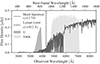 |
Fig. 1. Illustration of a mock spectrum with the U-band (LyC) and V606 (non-ionising UV) filters marked by the shaded areas. The Lyman limit is indicated with the vertical dashed black line. The fundamental observable, the LyC–to–non-ionising–UV flux ratio, ℛobs (see Sect. 2.2) measures the flux captured by the U-band (left) divided by the flux captured by the V606 filter (right). To ensure that the U-filter is always capturing flux short-ward of the Lyman limit, and is thus measuring ionising photons, we imposed a lower redshift bound of z = 3.35 on the galaxy sample. This mock spectrum was obtained from the intrinsic BPASS spectrum that was fitted to the stacked VANDELS spectrum in Begley et al. (2022) (see Sect. 3.2). The flux below the Lyman limit was attenuated according to an assumed fesc = 20%, whilst dust attenuation was applied to the non-ionising region using the Reddy et al. (2016b) dust curve and a value of AUV = 2.3. The full spectrum was multiplied with a simulated IGM transmission (exhibiting a transmitted fraction of 14% through the U filter; see Sect. 3.3). |
Lastly, targets with significant contamination in the imaging data from nearby companion objects were removed and potential AGN were excluded, reducing the final sample to 148 galaxies. The distribution of redshifts is mostly uniform within the selected range displaying a median of z = 3.58, while the distribution of stellar mass exhibits a median of log(M*/M⊙) = 9.5 with a range spanning from 8.6 to 10.5. For more details regarding the final sample selection and cleaning, we refer to Begley et al. (2022), where the distributions of redshift and stellar mass for the final sample are also displayed.
2.2. The observed LyC–to–non-ionising–UV flux ratio
The observed flux ratio of LyC to non-ionising UV, ℛobs, was obtained with imaging in the U-band and the V606 filter, and is defined as
 (1)
(1)
where ⟨fU⟩ and ⟨fV606⟩ are the flux densities per unit frequency measured within 1.2-arcsec diameter apertures. In Fig. 1, this corresponds to the flux captured in the dark grey filter (below the Lyman limit) divided by the flux captured in the light grey filter (above the Lyman limit).
We refer to Begley et al. (2022) for details regarding the preparation of the imaging data, which includes PSF-homogenisation, astrometry calibration and sky-subtraction. These steps were taken to ensure that the aperture photometry can be directly compared between the two filters, which entails the apertures capturing the same fraction of total flux for each object.
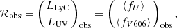
The distribution of ℛobs for the final sample of 148 star-forming galaxies is displayed in Fig. 2. Within our framework, it is this distribution that provides the main observational constraint on estimations of the escape fraction and, consequently, the distribution of the escape fraction across the galaxy population.
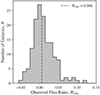 |
Fig. 2. Distribution of the observed LyC–to–non-ionising–UV flux ratio, ℛobs, exhibited by our final sample of 148 star-forming galaxies (see Sect. 2). The dashed line marks the median observed flux ratio of the sample. This distribution constitutes the observed data in our Bayesian inference framework (see Sect. 4), and thus provides the fundamental observational constraint on estimates relating to the escape fraction. The figure was adapted from Begley et al. (2022). |
3. Modelling framework
In Sect. 3.1 we introduce a forward model which relates the escape fraction to the observable LyC–to–non–ionising–UV flux ratio, ℛobs (see Sect. 2.2). This model requires a set of additional parameters,  , which are related to, respectively, the intrinsic ionising photon emission, the optical depth for ionising photons along a given sightline through the IGM, and dust attenuation in the non-ionising UV. These parameters are described separately in Sects. 3.2, 3.4, and 3.3.
3.1. Forward model for the escape fraction
We employed the physically motivated, forward model presented by Begley et al. (2022), which relates the observable flux ratio, ℛobs, to the escape fraction of ionising photons, fesc:
 (2)
(2)
Here ℛobs and ℛint are, respectively, the observed and intrinsic LyC–to–non–ionising–UV flux ratios (see Eq. (1));  is the line-of-sight transmitted fraction of ionising photons through the IGM and circumgalactic medium (CGM) integrated through the U-band filter; and AUV is the dust attenuation measured at the effective wavelength of the V606 filter.
In Fig. 1, we show a mock spectrum that helps visualise how the different components of Eq. (2) affect ℛobs compared to its intrinsic counterpart, ℛint. The escape fraction will reduce the observed flux at wavelengths below the Lyman limit (≃912 Å) (decreasing ℛobs). Similarly, the absorption of ionising photons by the IGM and CGM, accounted for in the model by an integrated transmitted fraction,  , will affect only flux measured in the ionising region (decreasing ℛobs). In contrast, the UV dust attenuation will reduce the observed flux at wavelengths above the Lyman limit (increasing ℛobs). The forward model intrinsically assumes that dust attenuation of ionising photons is contained in the escape fraction parameter, fesc, and thus AUV only impacts the non-ionising flux.
Modelling the escape fraction through a flux ratio between the LyC and the non-ionising UV band reduces the modelling complexity and facilitates determining a prior probability distribution for the intrinsic flux ratio (see Sect. 4.1), since we avoid the need to fit for the normalisation of the star formation history (SFH) when fitting the intrinsic spectral energy distribution (SED; see Sect. 3.2). Furthermore, the scaling ensures that the inference of the escape fraction is comparable for galaxies at (slightly) different redshifts since the resulting displacement of the rest-frame wavelength of the U-band and V606 filter, and thus the energies of the photons captured will affect both filters similarly. Anchoring the observation of the LyC flux, which is prone to absorption from intervening neutral hydrogen, to another more readily detectable region of the spectrum thus makes for a more reliable measurement. The ionising photons in the LyC are predominantly produced by OB stars, whose spectra are known also to dominate the UV region. Fluxes from these regions are therefore closely related, and a ratio between the two becomes practical for the analysis.
3.2. The intrinsic LyC–to–non-ionising–UV flux ratio
The intrinsic flux ratio of LyC to non-ionising UV, ℛint, is defined similarly to its observed counterpart (see Sect. 2.2 and Eq. (1)). It is computed from the intrinsic SED, whose shape is determined by the properties of the underlying stellar population. In the analysis of Begley et al. (2022), ℛint was determined by fitting Binary Population and Spectra Synthesis (BPASS) (Eldridge et al. 2017) stellar population models to a composite rest-frame far-ultraviolet continuum spectrum of the VANDELS sources, following the method of Cullen et al. (2019). This was based on a stellar metallicity of ≃0.07 Z⊙, and assuming a 100 Myr constant star formation history, ℛint for the individual galaxies varied between 0.17 − 0.20 (depending on the redshift).
Here, we relaxed these assumptions and allowed for greater variation of ℛint by expanding the star formation timescales and stellar metallicities of the intrinsic spectrum. We allowed for stellar metallicities in the range 0.01 − 0.2 Z⊙, constant star formation timescales > 20 Myr, and an upper-mass initial mass function (IMF) cutoff between 100 M⊙ and 300 M⊙. The resulting range of intrinsic ratios is 0.17 ≤ ℛint ≤ 0.38. We note that ℛint can, in principle, be larger than 0.38 at < 20 Myr, but we do not find strong evidence for such young ages in the individual VANDELS spectra.
3.3. IGM and CGM transmission
At the redshift of our sample, it is the absorption of ionising photons by the intervening neutral hydrogen that has the largest influence on the derived value of the escape fraction, fesc, and consequently its distribution. We see this in Eq. (2) as the complete degeneracy between the parameters fesc and  , which, mathematically, both denote a fraction that linearly reduces the value of the observed flux ratio, ℛobs, compared to the intrinsic flux ratio ℛint. Since we measure ℛobs with photometry, we are interested in the average fraction of ionising photons that are captured by our LyC filter, the U-band. We therefore let
  denote the average transmitted fraction of ionising photons, for a given sightline to a galaxy, integrated through the U-band filter (to remove the wavelength dependence).
The optical depth,  , which determines the transmitted fraction of ionising photons within the wavelength range of the U-band, is dependent on the spatial distribution of neutral clouds in the IGM, the HI column density of those clouds, and the redshift at which the photons are emitted. It will therefore vary significantly from one sightline to another and between different galaxies. Since it is not possible to map the exact column densities and spatial distribution of neutral hydrogen clouds along the line of sight to each galaxy, we accounted for the transmitted fraction in a probabilistic manner. To include both the IGM and CGM contribution to the transmission of LyC photons, we utilised transmission curves generated by Begley et al. (2022) using the parametrisation for the column density and redshift distribution of HI clouds given in Steidel et al. (2018). For six separate redshift bins (z = 3.4, 3.5, 3.6, 3.7, 3.8, 3.9), we generated 10 000 individual sightlines and integrated them through the U-band filter. For each redshift bin, we were thus provided with a distribution of the average transmission of LyC photons trough the LyC filter. We utilised these distributions (see Fig. 7 in Begley et al. 2022) as priors on the integrated transmitted fraction,
  , in the Bayesian framework introduced in Sect. 4.
3.4. UV dust attenuation
After the effects of the IGM and CGM, the UV dust attenuation, AUV, is the model parameter with the largest systematic influence on the escape fraction, fesc. In this context, it is defined as the dust attenuation in the rest-frame effective wavelength of the V606 filter (λeff, V606 = 5776.43 Å, corresponding to a typical rest-frame wavelength of ≃1300 Å for our final sample of galaxies (Begley et al. 2022).
The level of UV attenuation was determined individually for each galaxy, by comparing the observed UV spectral slope, βobs, with the spectral slope of the intrinsic SED model (βint = −2.44 ± 0.02; see Sect. 3.2 and Begley et al. 2022 for details of the fitting of an intrinsic model). The observed spectral slopes were determined by fitting a power law to each of the UV VANDELS spectra over the wavelength range 1300 − 1800 Å, within the continuum windows specified by Calzetti et al. (1994), obtaining an average of ⟨βobs⟩= − 1.26 ± 0.04 for the final galaxy sample. The attenuation at λ = 1600 Å was determined from the spectral slopes, using the relation: A1600 = 1.28 ⋅ (βobs − βint), which assumes an attenuation curve slope intermediate between a Calzetti and SMC law (see Begley et al. 2022 for details). The conversion to the UV dust attenuation, AUV, has a slight redshift dependence as the rest frame position of the effective wavelength of the V606 filter will vary depending on the redshift of the galaxy, but is roughly found by: AUV ≃ 1.2 ⋅ A1600.
4. Bayesian inference
To estimate the distribution of escape fractions across the population of galaxies in our sample, we adopted a two-level hierarchical Bayesian inference framework (see Hoff 2009; Lee 2012 for a general introduction to hierarchical models and Sonnenfeld & Leauthaud 2018; Wen et al. 2023 for examples of astrophysical implementation). With this hierarchical framework, we can combine information from individual galaxies to infer population-level parameters related to the distribution.
In Sect. 4.1, we describe the mathematical framework of the individual-galaxy-level inference, while Sect. 4.2 details how the individual layers are combined hierarchically. Section 4.3 proposes four different, physically motivated parametrisations of the distribution of the escape fraction, and implements these into the general, hierarchical framework described in the previous section. Finally, Sect. 4.4 recounts the general configurations used for sampling the probability distribution with a Markov chain Monte Carlo (MCMC) algorithm.
Using Bayesian inference, we can incorporate prior knowledge in the framework, which becomes particularly useful when including the integrated transmission through the IGM and CGM. While we are unable to measure the true transmitted fraction of ionising photons for every line of sight, we do have the probability distributions of the integrated transmission in various redshift bins (see Sect. 3.3). The Bayesian framework allows us to draw upon this information in the form of a prior probability distribution.
4.1. Inference of individual galaxy parameters
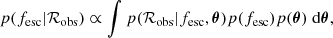
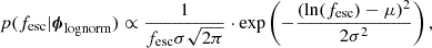
At the individual galaxy level, we want to obtain the posterior distribution of the escape fraction, fesc, given the observed data: the LyC–to–non–ionising–UV flux ratio, ℛobs. We can express the posterior probability of the escape fraction for one galaxy, p(fesc|ℛobs), using Bayes’ theorem,
 (3)
(3)
where we have omitted the subscript i, which otherwise denotes each of the N individual galaxies. Here,  is the set of additional model parameters needed in the generative model (see Eq. 2). Since we focused on the escape fraction in this analysis, we refer to θ as nuisance parameters and integrated over them in the expression above to obtain the marginal distribution. p(ℛobs|fesc, θ) is the likelihood expressing how probable the observed data, ℛobs, is, given the free parameters fesc and θ. p(fesc) is the prior on the escape fraction and
  is the prior on the nuisance parameters.
We assumed the likelihood function is normally distributed such that the likelihood for a given galaxy is
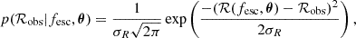 (4)
(4)
where σR is the observation error on the flux ratio, ℛobs, and ℛ(fesc, θ) denotes the modelled flux ratio as obtained with Eq. (2).
When adopting a Bayesian approach, we furthermore need to specify prior distributions for the free parameters: the escape fraction, fesc, and the 3 nuisance parameters contained in θ.
-
For the prior on the escape fraction, we defined p(fesc) to be uniform between 0 and 1.
-
We assumed a uniform prior on the intrinsic LyC–to–non–ionising UV flux ratio, ℛint within a range that is redshift-dependent and determined from fitting stellar population models to the stacked VANDELS spectra (see Sect. 3.2 for more details). The full prior range, for all redshifts in our galaxy sample, spans 0.17 ≤ ℛint ≤ 0.38.
-
For the integrated transmitted fraction,
 , we used priors generated by Begley et al. (2022) from the distribution of sightlines described in Sect. 3.3. These were obtained by performing a bounded (to the domain
  ) kernel density estimation (KDE)1 (Jones 1993) of the distribution for each of the 6 redshift bins. For each galaxy, we used its spectroscopic redshift as a fixed input to determine which of the 6 numerical priors,
  , to use. The prior probability assigned to a sampled transmission was determined by interpolating the finite-resolution priors described here.
 -
The prior on the dust attenuation, p(AUV), was assumed to be a normal distribution with mean and standard deviation given by the fits to the UV continuum slope of each galaxy. Here, we assumed a fixed value of βint, determined from fits to the stacked spectra (see Sect. 3.2), and an attenuation curve slope intermediate to a Calzetti and SMC curve (see Sect. 3.4).
We provide a graphical representation of the inference setup in Fig. 3. The inference of individual galaxy parameters, described in this section, is displayed within the depicted main box (denoted “Galaxy i” in the illustration). Notice, however, that the prior on the escape fraction is predetermined for the inference of individual galaxy parameters which we are describing here.
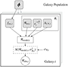 |
Fig. 3. Graphical representation of the two levels in the hierarchical Bayesian inference framework. The method of inference for individual galaxy parameters (see Sect. 4.1) is contained within the main box (denoted Galaxy i), while the full figure includes the hierarchical extension to the Bayesian network incorporating the population parameters (see Sect. 4.2). The grey outlines of multiple boxes in the background indicate the conditional independence between individual galaxy observations. The filled squares denote free sampled parameters, while the rectangle with a solid border denotes a deterministic node (the value is unambiguously determined from the input parameters and Eq. 2). The rectangle with the dashed border denotes a probability distribution with which the likelihood of the observed data, denoted with a circle, is evaluated. The observational error on ℛobs, σℛ is a fixed input to the model. |
4.2. Hierarchical inference of population parameters
This study aims to characterise the distribution of the escape fraction for our sample, p(fesc|ϕ), where we have introduced a set of population parameters, ϕ, to parametrise the distribution. At the population level, we want to obtain a posterior distribution of the set of parameters, ϕ, given the observed data (i.e. the observed flux ratio measurements for the full sample of N galaxies, {ℛobs}). We keep the notation general in this section, reviewing the relevant equations with the use of a non-specified set of parameters, ϕ, and defer the mathematical parametrisations of ϕ for four different model distributions to Sect. 4.3 along with their physical interpretation.
For one observation (i.e. one galaxy observation, corresponding to one box in Fig. 3), the posterior distribution of ϕ is described by
 (5)
(5)
where i denotes the galaxy in question. p(ϕ) is the prior on the population parameters – which will be specified depending on the different parametrisations introduced in Sect. 4.3. p(ℛobs, i|fesc, i, θi) is the likelihood of the observed data given the free local parameters (fesc, i and θi) and our model (Eq. 2). Finally, p(fesc, i|ϕ) is the prior on the galaxy-individual escape fractions as determined by the population distribution described by the sampled ϕ. Like the population prior, p(ϕ), the prior on the escape fraction is also dependent on the choice of model distribution, and we therefore refer to Sect. 4.3 for implementation details.
In Fig. 3, we visualise how the individual-galaxy-level and population-level parameters are connected in this hierarchical Bayesian inference framework. First, a set of population parameters, ϕ, is sampled, which defines a prior distribution of escape fractions, from which we sample an escape fraction for each galaxy. Following the methodology for inferring individual galaxy parameters described in Sect. 4.1, we obtain samples of the posterior distribution of the population parameters as constrained by one galaxy: p(ϕ|ℛobs, i).
We can combine the inference from a set of conditionally independent observations (i.e. individual galaxies) by multiplying the individual posteriors (Eq. (5)). The prior on the set of population parameters is, however, only applied once, since this term should only be invoked on the population level (i.e. outside the individual galaxy boxes in Fig. 3). The full expression for the posterior distribution of the population parameters, ϕ, given the full set of N observations, {ℛobs}, thus becomes (after marginalising over nuisance parameters θi)
 (6)
(6)
We argue that we can replace the individual likelihoods, p(ℛobs, i|fesc, i), in Eq. (6) with the corresponding posterior distribution of the galaxy-specific escape fraction, p(fesc, i|ℛobs, i), from the individual galaxy inference, defined in Eq. (3) (see Sect. 4.1). The individual likelihoods we are interested in for Eq. (6) are defined as (marginalised over the nuisance parameters θi)
 (7)
(7)
For the inference of individual galaxy parameters, the prior on fesc, i is uniform and therefore corresponds to scaling p(fesc, i|ℛobs, i) by a constant p(fesc, i). The evidence, p(ℛobs, i), is constant for the choice of model (Eq. (2)), and will therefore, similarly, only result in a scaling of p(fesc, i|ℛobs, i). This implies that p(ℛobs, i|fesc, i)∝p(fesc, i|ℛobs, i), and the proposed replacement is therefore valid due to the normalisation-insensitive property of an MCMC algorithm. Note that we only obtain samples of the posterior distribution with an MCMC algorithm, and we therefore have to perform a KDE on the set of posterior samples for each p(fesc, i|ℛobs, i) to efficiently use the individual posteriors as likelihoods in the hierarchical framework.
4.3. Population distributions
In this section we introduce four different parametrisations for the population distribution of escape fractions, namely, (i) a constant escape fraction across the population of galaxies (following Begley et al. 2022), (ii) a lognormal distribution, (iii) an exponentially decaying distribution, and (iv) a bimodal distribution consisting of a constant and a normal component.
Here, we specify the set of population parameters, ϕ, the prior on the population parameters, p(ϕ), and provide the functional form of the population distribution (which assumes the purpose of a prior), p(fesc, i|ϕ), for the four different model distributions. The distributions are all physically motivated and in Fig. 4 we demonstrate how each is connected to the two main mechanisms with which ionising photons escape their host galaxy: a density-bounded and/or an ionisation-bounded scenario.
 |
Fig. 4. Four physically motivated distributions of the escape fraction placed on a scale to indicate their connection to the two simplified physical pictures of how ionising photons may escape the ISM of their host galaxy. The blue picture represents the density-bounded leakage mechanisms, while the green scenario is where ionising photons escape through ionised low-density channels. In both scenarios the arrows indicate the escape of LyC photons. The constant distribution represents a scenario where all galaxies have the same physical conditions, and LyC photons escape via purely density-bounded leakage from Strömgren spheres with the same column density, while the bimodal model can represent an ionisation-bounded scenario where leakage is mostly strongly sightline dependent and/or a density-bounded scenario that is strongly time variable. The log-normal and exponential distribution represent complex mixtures of the two main leakage mechanisms. |
Common for the four parametrisations, is that the escape fraction, fesc, is defined to be between 0 and 1. The distribution of escape fractions, p(fesc, i|ϕ), must therefore be normalised in this interval. For simplicity, we omit this normalisation of the truncated distribution in the notation for the four different distributions described in the subsequent sections.
4.3.1. Constant distribution
This model assumes that the escape fraction, fesc, is the same for the entire galaxy population. The distribution of escape fractions, p(fesc|ϕ), will thus be described by a Dirac-delta function placed at fesc = μ. The set of population parameters for this model is thus given by a single parameter, ϕconst = μ, and the distribution takes the functional form
 (8)
(8)
where δ denotes the Dirac-delta function. We assumed a uniform prior between 0 and 1 on μ.
The constant distribution represents the case where the fraction of LyC photons escaping is the same for different galaxies such that a single value of the escape fraction is descriptive of all observations in our sample. In this scenario the leakage of ionising photons is exclusively driven by a density-bounded scenario, assuming all galaxies have Strömgren spheres of the same density. In the density-bounded scenario, surrounding hydrogen has been ionised by LyC flux from a powerful star formation period in the centre of the galaxy. In this picture, a fraction of the subsequently produced ionising photons is used to balance the rate of recombination, while the remaining fraction of LyC photons is allowed to escape the galaxy’s ISM.
4.3.2. Log-normal distribution
Here, the population distribution of escape fractions, p(fesc|ϕ), is given by a log-normal distribution, parametrised by
 (9)
(9)
where the population parameters are ϕlognorm = (μ, σ), which describe, respectively, the mean and standard deviation of the natural logarithm of the variable fesc.
To retain the characteristic feature of a log-normal distribution within the domain of the escape fraction, we required that the mode, M = exp(μ − σ2), is always between 0 and 1. This implies that the prior on the standard deviation should restrict σ to the range as determined by the sampled μ and inserting M = 0 and M = 1 in the expression: 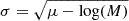 . By definition, we need σ > 0 and we therefore required μ − log(M) > 0 and M > 0. Furthermore, to avoid computational overflow we limited σ > 0.01 and for simplicity assumed 0 < μ < 5. We employed uniform priors for both parameters in the specified ranges. In practice, we sampled log10(σ) to more effectively explore the parameter space.
The log-normal distribution represents a complex mixture of leakage mechanisms. In particular, the distribution of escape fractions in this physical picture could arise from an underlying log-normal distribution of neutral hydrogen column densities in the galaxy’s ISM though simulations typically predict more complex distributions (Ma et al. 2020; Mauerhofer et al. 2021). In this distribution, the escape fraction cannot be zero, essentially ruling out a purely ionisation-bounded scenario or strongly time-variable leakage.
4.3.3. Exponential distribution
Here, we assume the population distribution of escape fractions, p(fesc|ϕ), is given by an exponentially decaying function, parametrised as
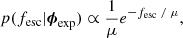 (10)
(10)
where μ > 0 is the scale parameter, which also describes the mean of the distribution. We required the mean escape fraction to be between 0 and 1 and therefore assumed a uniform prior on this interval. In practice, we sampled the parameter in logarithmic space and thus enforced a uniform prior between −3 and 0 on the transformed parameter log10(μ).
Similar to the log-normal distribution, the exponential distribution represents a complex mixture of leakage mechanisms and a potentially exponential distribution of HI column densities. fesc = 0 is possible in this model, allowing for strongly time- and/or sightline-variable LyC leakage.
4.3.4. Bimodal distribution
In the bimodal model distribution, we assume the population distribution of escape fractions, p(fesc|ϕ), is made up of two components: (i) a fraction, w, of the galaxies in the population is assumed to exhibit a zero escape fraction (i.e. no LyC photons escape from these galaxies). This component is described by a Dirac-delta function placed at fesc = 0, and weighted by w. (ii) the escape fraction of the remaining galaxies in the population is described by a normal distribution, centred at μ with standard deviation σ. The set of population parameters for this parametrisation is thus given by ϕbimodal = (w, μ, σ), and the population distribution is described by
 (11)
(11)
where δ denotes the Dirac-delta function and 𝒩 denotes the normal distribution.
The prior on the population parameters is given by: p(ϕ) = p(w)p(μ)p(σ). We assumed the prior on the weight parameter, w, is uniform between 0 and 1 such that the full distribution of escape fractions normalises to unity (after truncating the normal distribution component). Furthermore, we assumed the mean, μ, of the normal distribution must be part of the domain of the escape fraction, and we thus assumed the prior to be uniform between 0 and 1 as well. Lastly, the standard deviation of the normal distribution, σ, should be positive. For computational efficiency, we restricted this parameter more and sampled it in logarithmic space. We used a uniform prior on the interval −3 ≤ log10(σ)≤0.
The two components of the bimodal distribution represent, respectively, a fraction of galaxies with zero escape fraction corresponding to galaxies where no LyC photons escape and a fraction of galaxies with higher escape fractions corresponding to observations where the line of sight coincides with a low-density channel in the surrounding hydrogen. As such, the bimodal distribution can represent an ionisation-bounded scenario with a small number of highly ionised low-density channels and/or a density-bounded scenario with strongly time variable star formation and LyC escape. In the latter case, galaxies are optically thin to LyC radiation for only a short timespan, for example, due to hard radiation fields and/or stellar or supernovae feedback, and optically thick the rest of the time.
4.4. Sampling configurations
To sample the various posterior distributions of interest, we employed the affine-invariant, ensemble, Markov chain Monte Carlo (MCMC) sampler emcee (Foreman-Mackey et al. 2013) with the default StretchMove, a Python implementation of the sampling algorithm originally proposed by Goodman & Weare (2010).
The walkers were initialised with positions in the parameter space drawn from the respective parameter priors, except for the integrated transmission values, which were initialised uniformly between 0 and 0.5 (instead of the full range spanning up to 1). The transmission priors were generated with a KDE of 10 000 sightline simulations, but for transmitted fractions closer to 1 we only have a few simulated sightlines and we enter a regime of low statistics (especially for higher redshifts). As a result, some of these priors exhibit local extrema that are unphysical artefacts resulting from low sampling. To avoid walkers getting stuck in a local, unphysical maximum we initialised the walkers closer to the true maxima found between 0 and 0.5.
We used 50 walkers, each sampling at least 10 000 positions in the parameter space. The number of steps was chosen so the chains were at least 100 times the longest integrated auto-correlation length, thus ensuring independent samples of all the free parameters. The number of samples discarded as the burn-in phase was computed as 2 ⋅ max(τ), where τ is a list of auto-correlation lengths for each of the sampled parameters, and we used every 0.5 ⋅ min(τ) step of the sampled chains.
Unless otherwise stated, we report inferred model parameters as the mode of the corresponding posterior samples along with the 68th per cent highest posterior density (HPD) interval.
5. Results
In this section we present our constraints on the distribution of escape fractions estimated from the observed flux ratios, {ℛobs}, from a sample of 148 star-forming (z ≃ 3.5) galaxies in the VANDELS survey (McLure et al. 2018; Pentericci et al. 2018; Garilli et al. 2021).
Section 5.1 presents an example of the constraining power on the escape fraction, fesc, and the nuisance parameters, θ, for two individual galaxies, while Sect. 5.2 describes the inferred constraints on the population distribution of escape fractions, p(fesc|ϕ), based on observations from all galaxies in the sample. Here, we provide constraints for the four different parametrisations of the distribution: constant, log-normal, exponential, and bimodal (all described in Sect. 4.3). Finally in Sect. 5.3, we compare the four model distributions and investigate their respective ability to reproduce the observed distribution of ℛobs in the galaxy sample.
5.1. Constraints on individual galaxy escape fractions
We use the framework for inferring individual galaxy parameters (see Sect. 4.1) to constrain the escape fraction, fesc, for each of the 148 galaxies in our sample. In Fig. 5, we show examples of the resulting posterior distributions (not explicitly marginalised over the nuisance parameters) for a robust detection (≥5σ) and a typical, non-detected galaxy in the U-band (≤1σ).
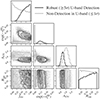 |
Fig. 5. Corner plot showing the 1D and 2D marginalised posteriors for the escape fraction, fesc; the integrated transmission through the U-band filter, |

Inspecting the marginalised posterior of the escape fraction (see the top panel of Fig. 5), we see that even for the galaxy with a robust ℛobs detection (dark grey), we are not able to tightly constrain the escape fraction. The posterior provides a lower limit on the escape fraction fesc > 0.38 from the 68 per cent HDP interval, consistent with previously reported values by Vanzella et al. (2010), Ji et al. (2020), where this source (Ion1) is extensively discussed (see also Saldana-Lopez et al. 2023). The case is even less informative for a typical non-detection (light grey), where the posterior samples the full domain of the escape fraction. These results indicate that observations from single galaxies do not individually exhibit much constraining power on the galaxy-individual escape fractions. In the next section, however, we will demonstrate how the constraining power on population-level parameters profits from combining observations of multiple galaxies.
5.2. Constraints on the population distribution of escape fractions
We used the general hierarchical inference framework, described in Sect. 4.2, to constrain the set of population parameters, ϕ, for each of the four parametrisations of the escape fraction distribution: (a) constant, (b) log-normal, (c) exponential and (d) bimodal (all described in Sect. 4.3). In Fig. 6, we display the resulting posterior distributions for the set of population parameters, ϕ, for each of the four models.
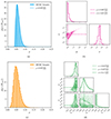 |
Fig. 6. 1D and 2D marginal posterior distributions of the set of population parameters, ϕ, for each of the four models described in Sect. 4.3. The dashed lines indicate the mode of the posterior samples, and values are reported as the mode with the 68 per cent HDP interval. Panel (a): 1D marginal posterior of the population parameter ϕconst = μ (blue), describing the constant escape fraction value most likely to describe all galaxies in the sample. Panel (b): Corner plot showing the 1D and 2D marginal posterior distributions of the set of population parameters ϕlognorm (pink), describing a log-normal distribution of escape fractions. Here μ and σ represent, respectively, the mean and standard deviation of the natural logarithm of the escape fraction. Panel (c): 1D marginal posterior of the population parameter ϕexp = μ (orange), which represents the scale parameter in an exponential distribution of escape fractions. Panel (d): Corner plot containing the 1D and 2D marginal posteriors for the set of population parameters ϕbimodal (green), which describes a bimodal distribution of escape fractions: w denotes the fraction of galaxies with a constant escape fraction equal to zero, while μ and σ describe the escape fraction of the remaining galaxies as being normally distributed. |
Panel (a) (of Fig. 6) shows the marginalised posterior distribution of the constant distribution’s population parameter, for which we report an inferred value of 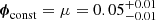 . This distribution assumes that all galaxies share the same value of the escape fraction and μ should therefore be interpreted as the most likely value of fesc to describe all galaxies, rather than the average of 148 individual values of the escape fraction. Our inferred value is fully consistent with the corresponding ⟨fesc⟩ = 0.05 ± 0.02 that was reported by Begley et al. (2022), using a similar approach.
We note here there are two key differences between our implementation and that of Begley et al. (2022), but both effects effectively cancel out to provide the same ⟨fesc⟩ result. Firstly, by including a variable intrinsic flux ratio, ℛint in our inference, we allowed higher values of ℛint compared to Begley et al. (2022), which translates to slightly lower values of the escape fraction, fesc. Secondly, we updated the KDE method used to obtain the individual fesc posteriors so they can be multiplied, obtaining the population posterior displayed in Fig. 6. We used a KDE bounded at 0 ≤ fesc ≤ 1, which is more robust for high fesc and cause a systematic shift to slightly higher fesc, contrary to Begley et al. (2022) who used only a lower bound on the KDE. Replicating the method in Begley et al. (2022) where ℛint is a fixed parameter, but with our updated KDE implementation, we find a slightly higher  compared to that presented by Begley et al. (2022).
Panel (b) (of Fig. 6) shows the 1D and 2D marginalised posterior distributions for the population parameters constituting the log-normal distribution. The set of population parameters is found to be  , describing, respectively, the mean and the standard deviation of the natural logarithm of the escape fraction. The expected value is E[fesc] = 0.29 (i.e. higher than for the constant distribution) because the shape of the log-normal distribution does not allow for fesc = 0, and thus produces nonphysical results as we will discuss in Sect. 5.3.
Panel (c) (of Fig. 6) shows the marginal posterior distribution of the scale parameter of the exponential model distribution. We find that  . The scale parameter, μ, also describes the mean escape fraction of the population distribution, p(fesc|ϕexp). The expected value is E[fesc] = 0.05 and is thus consistent with the constant model.
Panel (d) (of Fig. 6) shows the 1D and 2D marginalised posterior distributions for the population parameters in the bimodal parametrisation. The set of population parameters is found to be  , denoting, respectively the fraction of galaxies with a constant zero escape fraction, and the mean and standard deviation of the normal component. The expectation value is E[fesc] = 0.05, fully consistent with both the constant and exponential model parametrisations.
While the expectation values of the four inferred escape fraction distributions mostly align well, this does not provide insight into the actual shapes of the distributions and how they may differ.
To visually compare the different models, in Fig. 7, we plot the median cumulative distribution function (CDF) of the escape fractions for each of the four models. The median CDF, for each model, was computed from the resulting distributions of 10 000 parameter-sets taken from the posterior samples2 displayed in Fig. 6. The median is shown in a solid line, while the shaded region marks the 16th and 84th percentile intervals.
 |
Fig. 7. Median cumulative distribution of the population distribution of escape fractions for each of the four models. For each model we (i) selected 10 000 parameter sets from the chains of posterior samples displayed in Fig. 6, (ii) evaluated the CDF of the distribution given by the selected population parameters on a grid of escape fractions, and (iii) computed the median of the 10 000 corresponding CDF values for each index of the escape fraction grid. The median is shown as a solid line, while the shaded region marks the 16th and 84th percentile intervals. For reference, we plot the CDF of a uniform distribution as a dashed line. |
The constant, exponential, and bimodal models all indicate that the majority (or all) of the galaxies in our sample exhibit low escape fractions (fesc < 0.1), which agrees well with the large number of non-detections in our sample (144 galaxies with S/N < 3). The log-normal distribution similarly predicts a majority of galaxies with lower escape fractions (50% of galaxies with fesc < 0.2), but predicts more galaxies with larger escape fractions compared to the other distributions.
5.3. Model comparison
We now aim to constrain which of the four distributions best describes our observations. Adopting an MCMC approach to infer the distribution of escape fractions, results presented in the previous section are inherently dependent on the chosen parametrisation of the distribution. To properly quantify whether an inferred distribution is capable of describing the observed data (the LyC–to–non–ionising–UV flux ratios of the galaxies, {ℛobs}), we performed a posterior predictive check (e.g. Gelman et al. 1996). We produced a mock ℛobs distribution based on the inferred escape fraction distribution and compared it to the observed data using a two-sample Kolmogorov-Smirnov (KS) test.
The KS test statistic is a measure of how much the two distributions differ (it reports the maximum difference between the two cumulative distributions) and a lower KS score will therefore indicate a better model. Together, the KS score and the sample size translates into a probability (p-value) of whether the two ℛobs distributions are samples from an identical population distribution. The significance level, α, corresponds to the desired minimum probability (i.e. when we set α = 0.10); we reject a model if a resulting mock ℛobs distribution exhibits less than a 10% probability of matching the observed distribution. Since the KS test is a non-parametric test, the p-value tests for any violation of the null-hypothesis, for example if the ℛobs distributions have different medians, different variances or different population distributions. It thus provides a flexible, yet powerful test that is furthermore independent of any binning of the data.
To produce the mock ℛobs distribution for each of our four models, we first sampled a set of population parameters from the posterior chains (displayed in Fig. 6) each defining a certain distribution of escape fractions. From this distribution, we sampled 148 escape fractions to produce a sample of mock galaxies with the same size as our true sample. To best emulate the real sample, we used the (for each galaxy) measured spectroscopic redshift, UV dust attenuation, AUV, along with the observed LyC–to–non–ionising–UV flux ratio, ℛobs, (and error σℛ) as parameters for creating a mock sample. The fitted intrinsic SED (described in Sect. 3.2) was then modified to produce an observed spectrum for each galaxy and ℛobs was extracted (see Appendix A for the full procedure of producing mock galaxy spectra and measuring ℛobs). We repeated this process 10 000 times, essentially producing 10 000 mock ℛobs distributions, for each of the four models presented in Sect. 4.3. These many distribution samples were then collapsed into one distribution with 10 000 × 148 samples, so we could perform a single KS test for each model and thus benefit from the self-normalising property of the KS test.
With such a large sample size, the sampling error is negligible and we choose to employ a somewhat large α = 10% significance level (compared to the conventional 5%) for rejecting the hypotheses of the distribution matching the observed data.
In Fig. 8, we display the empirical CDF (eCDF) of the real, observed sample of flux ratios, ℛobs, together with the corresponding eCDF for each of the four model distributions. Here, the KS score for each model represents the largest vertical distance between the two. From visual inspection it is evident that the log-normal model performs worst. It significantly overestimates the number of galaxies with observed flux ratios above ℛobs > 0, which is related to this model predicting more galaxies with larger escape fractions compared to the other models, as we saw in Fig. 7. Furthermore, we see that the bimodal model slightly overestimates the number of non-detections with ℛobs around 0.
 |
Fig. 8. Posterior predictive test of the four models. (Top) Visual illustration of the KS score, which measures the maximum difference between the eCDF of the observed flux ratios, ℛobs (plotted in black), and the eCDF of a simulated ℛobs distribution dependent on respectively the constant, log-normal, exponential, and bimodal model distribution of the escape fraction as inferred from the Bayesian framework. (Bottom) Residual (the model eCDF minus the data eCDF). |
We provide the KS test score and the associated p-value for each of the four model distributions in Table 1. At a 10% significance level, we reject the log-normal and bimodal fesc distributions as good descriptions of our observed flux ratios, ℛobs, while both the constant and exponential models exhibit plausible p-values. However, as we argue in Sect. 6, the exponential model is likely the best representative of the escape fractions of our galaxy sample.
KS test results.
5.4. Correlation with the UV continuum slope
We investigated how the escape fraction correlates with the UV continuum slope, β (a proxy for dust and HI column density of the ISM in the galaxy), for our best-fitting model: the exponential distribution.
We split the full galaxy sample in half at the median value of the UV slope, β = −1.30, creating two subsamples (red and blue galaxies) each consisting of 74 galaxies. For each of these samples, we used the hierarchical Bayesian inference framework to determine the population distribution of escape fractions as parametrised by the exponential distribution.
Figure 9 shows the resulting CDF of the escape fraction distribution for, respectively, the full sample, the red subsample, and the blue subsample. We find that there is a correlation between higher escape fractions and lower UV slope (bluer galaxies), indicating that galaxies with lower levels of UV dust attenuation display a larger escape fraction. This trend is consistent with the results reported in Begley et al. (2022) as well as findings from lower redshift studies (e.g. Chisholm et al. 2022).
 |
Fig. 9. Cumulative distribution of the escape fraction as parametrised by the exponential scale parameter, ϕexp = μ, inferred for, respectively, the full sample (grey), the galaxy subsample with lowest UV slopes (blue), and the subsample with highest UV slopes (red). The inset shows the corresponding inferred posterior distribution, where the dashed line marks the mode of the distribution. |
6. Discussion
In Sect. 6.1, we discuss which escape fraction distribution is best representative of our sample and what implications it has for our understanding of how ionising photons escape their host galaxy. We compare our best model distribution with predictions from simulations in Sect. 6.2. For a discussion on systematic uncertainties associated with modelling the escape fraction with Eq. (2), we refer to Sect. 5 in Begley et al. (2022).
6.1. What is the best representation of the population distribution of the escape fraction?
This work presents the first constraints on the shape of the escape fraction distribution in the galaxy population at z ∼ 3 − 4. Previous work by Vanzella et al. (2010) measured median values given different escape fraction distributions but did not distinguish between the models. Here we have taken the important next step in performing a model comparison to assess which model best fits the observations.
The constant and exponential model of the escape fraction distribution both exhibit acceptable p-values when employing a KS-test, and we therefore cannot reject either of their abilities to match the observed data. Here we argue that, physically, the ionising photon escape fraction should not be a constant across the galaxy population and thus the exponential model should be the best description of the data.
Our sample of galaxies includes two objects with robust LyC detections (individual U-band flux detections with ≥5σ significance), for one of which we presented the constraints on the galaxy-individual escape fraction in Fig. 5. The 95 per cent HPD interval places a lower limit on the escape fraction for this galaxy at fesc > 0.38, clearly incompatible with the physical picture proposed by the constant model, where we inferred a constant escape fraction of  (see panel (a), Fig. 6). Furthermore, these 2 objects have previously been reported in the literature (e.g. Vanzella et al. 2010; Ji et al. 2020; Saxena et al. 2022) which finds similar lower limits on the galactic scale escape fractions that conflict with the scenario described by the constant model. Therefore, we argue, that the constant distribution cannot be the most representative model. This is also in agreement with findings from other surveys which indicate that the escape fraction is far from constant in all galaxies (e.g. Steidel et al. 2018; Pahl et al. 2021; Flury et al. 2022a).
Our inferred, exponential distribution of the escape fraction points towards complex LyC photon leakage scenarios, where most galaxies exhibit similar, non-zero, but low escape fractions (fesc < 0.1) while a few galaxies exhibit high leakage of LyC photons. This may reflect a broad distribution of ISM HI column densities (Trebitsch et al. 2017; Ma et al. 2020; Mauerhofer et al. 2021) and strongly time and/or sightline variable LyC leakage, where for a high fraction of time and/or sightlines galaxies are optically thick to LyC photons. This picture aligns well with the findings of lower redshift surveys, which, depending on the study and sample, report either the density-bounded or ionisation-bounded scenario as being the most plausible. The scenario where LyC photons leak primarily through channels in an ionisation-bounded ISM (Gazagnes et al. 2020), probably carved by photo-ionised outflows (Amorín et al. 2024) after the onset of supernovae (Bait et al. 2024) is supported by observations of down-the-barrel absorption lines in the UV (Gazagnes et al. 2018; Saldana-Lopez et al. 2022). However, in the most extreme leakers, a density-bounded scenario is more plausible as evidenced by a highly ionised ISM traced by high O32 ratios (Izotov et al. 2021; Flury et al. 2022b). The dominance of each scenario at different fesc regimes might be in agreement with the underlying exponential fesc distribution found in this study.
Our sample only presents a few actively LyC leaking galaxies, explaining why a constant model can statistically reproduce the data and why the parameters describing the normal component of the bimodal model, ϕbimodal = (μ, σ), are difficult to constrain (see Fig. 5.2, panel (d)). We find support for the exponential model being the best representation of the population distribution of the escape fraction in our sample, but the analysis would benefit from a larger sample to better constrain the respective model parameters - in particular, to better capture the tail of the distribution representing LyC leakers.
6.2. Comparison with simulations
To gain physical insight into the inferred escape fraction distribution we can compare to predictions from simulations. There exist multiple frameworks for simulating reionisation, all reporting some distribution of the escape fraction (e.g. Kimm & Cen 2014; Ma et al. 2020; Barrow et al. 2020; Paardekooper et al. 2015; Rosdahl et al. 2022; Kostyuk et al. 2023; Katz et al. 2023; Choustikov et al. 2024). Nonetheless, to properly compare any distribution with our results, we need to identify simulations using: (i) a similar definition of the escape fraction as the one adopted in this work and (ii) a galaxy sample closely analogous to the final sample used for inferring the exponential distribution in this study.
Most simulations report the angle-averaged, cosmic escape fraction of LyC photons, while in this work, we used observational data and are thus limited to sightline-dependent escape fractions. The SPHINX suite of cosmological radiation-hydrodynamical simulations of reionisation (Rosdahl et al. 2018, 2022; Katz et al. 2023), however, provides the LyC escape fraction (measured at rest frame wavelength 900 Å) for 10 different sightlines for each galaxy in the simulation and is therefore a suitable candidate for comparison with our results.
We made the following selection of SPHINX galaxies to best emulate our sample:
-
The SPHINX galaxies present redshifts spanning from 4.64 < z < 10, while our sample exhibit redshifts in the range 3.35 < z < 3.95. We selected SPHINX galaxies with z < 5.5 for the comparison.
-
The SPHINX galaxies are generally lower mass than our sample displaying 6.51 < log(M*/M⊙) < 10, while our sample shows masses in the range 8.66 < log(M*/M⊙) < 10.44. We selected all SPHINX galaxies within the mass range of our sample. To avoid an otherwise considerable overweight of lower mass galaxies compared to our sample, we further down-sampled galaxies with log(M*/M⊙) < 9 by 90 per cent (i.e. keeping 10 per cent).
-
Each SPHINX galaxy has ten different sightlines available. We selected galaxies with sightlines where the observed optical UV β-slope is within the range of our galaxy sample such that −2.68 < βobs < 0.43. Note, however, that SPHINX galaxies are generally bluer (exhibiting lower β-slopes) than our sample.
In Fig. 10, we display the analytical CDF of the distribution of the LyC escape fraction as inferred from our exponential model along with the empirical CDF from 1139 SPHINX sightlines. While the shape of the CDFs hold some similarities, the distributions do not match and the simulations underpredict the escape fraction relative to our result.
 |
Fig. 10. Cumulative distribution of the population distribution of the escape fraction. Shown are the median CDF for the exponential model inferred in this work (in orange; the shaded region marks the 16th and 84th percentile interval) and the eCDF for a selection of SPHINX galaxies (in black) with somewhat similar properties to our observed sample. For context, the CDF for selections of red high-mass galaxies and blue low-mass galaxies in SPHINX are plotted. All selections are described in Sect. 6.2. |
Accounting for the differences in galaxy properties between the compared samples, the distributions are predicted to be less consistent than what is shown in Fig. 10. For one, the redshift range of our sample is lower than those exhibited by the SPHINX galaxies. Rosdahl et al. (2022) predicts (using the SPHINX suite of simulations) a correlation between redshift and global escape fraction, indicating that simulated galaxies with lower redshifts would exhibit even lower escape fractions. In addition, the SPHINX galaxies exhibit an overweight of blue (lower UV β-slopes) compared to our sample, which suggests SPHINX galaxies should display a larger mean fesc compared to the mean of our inferred exponential distribution.
In Fig. 9, we demonstrated that bluer galaxies have an escape fraction distribution shifted to higher values. In one further attempt to match any selection of SPHINX galaxies to our inferred exponential distribution, we select blue low-mass galaxies (6.51 < log(M*/M⊙) < 9.5, −2.68 < βobs < −2) and red high-mass galaxies (9.5 < log(M*/M⊙) < 10.63, −2 < βobs < 0.68) from the full SPHINX catalogue (still imposing z < 5.5) and plot their eCDF (displayed in Fig. 6.2). We find the blue low-mass galaxies exhibit a distribution shifted towards larger escape fractions, with mass being the dominant driver of this trend (Rosdahl et al. 2022). However, even this sub-sample with higher escape fractions in the SPHINX sample is not able to reproduce our inferred exponential distribution and still underpredicts the escape fraction.
To better compare simulations with observational constraints on the distribution of the escape fraction in the future, we encourage simulations to report sightline galactic-scale escape fractions for galaxies at lower redshift.
7. Conclusions
In this work we used data from the VANDELS spectroscopic survey (McLure et al. 2018; Garilli et al. 2021) to measure the distribution of the ionising photon escape fraction from 148 star-forming, reionisation-era analogue galaxies (3 < z < 4). This sample of galaxies was originally presented in Begley et al. (2022).
We developed a hierarchical Bayesian inference framework to infer the distribution of the ionising photon escape fraction from the ratio of LyC to non-ionising UV flux, as measured by broadband photometry. Our method incorporates careful treatment of the IGM and CGM transmission of ionising photons, and accounts for the effects of dust attenuation in the UV and the uncertain intrinsic ratio of ionising to non-ionising UV flux. Within this framework, we have tested three physically motivated distributions beyond the constant model developed by Begley et al. (2022): an exponential, a log-normal, and a bimodal parametrisation of the population distribution of escape fractions.
The main results of this study are summarised as follows:
-
The constant, exponential, and bimodal population distributions all recover the same expected value of fesc = 5%, consistent with the result of Begley et al. (2022), while the log-normal parametrisation finds an expected value of 29%.
-
Using a posterior predictive test, we find that the exponential and constant distributions are best at reproducing the measured LyC–to–non-ionising–UV flux ratios of our galaxy sample. The performance of the two distributions is, however, not statistically distinguishable (with the current sample size). The bimodal and log-normal distributions are ruled out with high significance.
-
We argue that the exponential distribution is most likely representative of the true distribution of the escape fraction in our sample. Unlike the constant model, the exponential distribution is consistent with individual constraints on the escape fraction obtained for two galaxies with robust (≥5σ) LyC detection in our sample, which place a lower limit on the escape fraction of fesc > 0.38. These constraints are consistent with values reported in the literature (see Vanzella et al. 2010; Ji et al. 2020; Saxena et al. 2022).
-
We find that the bimodal model of the distribution of the escape fraction in our sample is disfavoured, implying that a purely bimodal escape of ionising photons, via strong sightline and/or time variability, is improbable.
-
We split our sample into two subsamples based on the UV continuum slope (β-slope) and repeated the full hierarchical inference scheme to infer an exponential distribution representative of each sample. We find that the escape fraction anti-correlates with the β-slope, such that bluer galaxies (lower β-slopes) are more likely to populate the high-end tail of the escape fraction distribution. In particular, we infer the scale parameter for blue and red galaxies as, respectively,
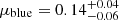 and
and 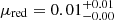 , compatible with the findings of Begley et al. (2022) and low-z LyC surveys (Chisholm et al. 2022).
 -
We compared the inferred exponential distribution of the escape fraction (with scale parameter
 ) to sightline escape fractions reported from the SPHINX suite of cosmological radiation-hydrodynamical simulations of reionisation (Rosdahl et al. 2018, 2022; Katz et al. 2023), but we find that the simulations underpredict the escape fractions relative to the results from our sample. While the galaxies in SPHINX and in our sample are not directly analogous, presenting (among other properties) different redshift ranges, based on the other predicted trends in the simulations even with a better-matched simulated sample the SPHINX distribution would remain inconsistent with our results.
Reproducing the line-of-sight escape fraction distribution can be a key test for the implementation of physical conditions and feedback mechanisms in simulations. Future studies would benefit from radiation-hydrodynamical simulations reporting line-of-sight specific escape fractions, in addition to the typically reported angle-averaged escape fractions. This would enable a more direct comparison with the observations and a better understanding of the physical processes responsible for the escape of ionising photons.
Our results also have important implications for the reionisation process itself. Models commonly assume a constant or deterministic escape fraction from galaxies during reionisation (Madau et al. 1999; Robertson et al. 2010; Park et al. 2019; Naidu et al. 2020; Muñoz et al. 2024). An exponential distribution implies that only a small fraction of sources may be contributing to reionisation at a given time, likely due to a combination of time and/or sightline variability. Thus, considering the escape fraction distribution may alleviate the ionising photon ‘budget crisis’ implied by recent JWST estimates of the ionising photon production efficiency (Muñoz et al. 2024).
We also demonstrated that the shape of the fesc distribution depends on the UV β-slope, with bluer galaxies having a distribution shifted to higher fesc. With larger samples it will be possible to constrain the escape fraction distribution parameters as a function of galaxy properties such as the SSFR, stellar mass, UV magnitude, and β-slope. This dependence on galaxy properties will be important for predicting the escape fraction distribution during the Epoch of Reionisation.
The boundary correction of the KDE was made with the linear_combination method (also known as generalised jackknifing) in pyqt-fit (https://github.com/KimiKreil/pyqt-fit)
Except for the constant model which by definition have a strictly vertical CDF and was therefore plotted using the corresponding quantiles of the sampled parameter ϕconst = μ.
Acknowledgments
We thank Joki Rosdahl for useful discussions and sharing the SPHINX fesc catalog. KCK and CAM acknowledge support by the Carlsberg Foundation under grant CF22-1322. CAM also acknowledges support by the VILLUM FONDEN under grant 37459. The Cosmic Dawn Center (DAWN) is funded by the Danish National Research Foundation under grant DNRF140. FC acknowledges support from a UKRI Frontier Research Guarantee Grant (PI Cullen; grant reference EP/X021025/1). This work made use of the following open-source software: Matplotlib (Hunter 2007), Numpy (Harris et al. 2020), SciPy (Virtanen et al. 2020), Astropy (Astropy Collaboration 2022), emcee Foreman-Mackey et al. (2013), pandas (The pandas development Team 2024), Corner (Foreman-Mackey 2016), and Numba (Lam et al. 2015).
References
- Aird, J., Coil, A. L., Georgakakis, A., et al. 2015, MNRAS, 451, 1892 [Google Scholar]
- Alavi, A., Colbert, J., Teplitz, H. I., et al. 2020, ApJ, 904, 59 [NASA ADS] [CrossRef] [Google Scholar]
- Amorín, R. O., Rodríguez-Henríquez, M., Fernández, V., et al. 2024, A&A, 682, L25 [NASA ADS] [CrossRef] [EDP Sciences] [Google Scholar]
- Astropy Collaboration (Price-Whelan, A. M., et al.) 2022, ApJ, 935, 167 [NASA ADS] [CrossRef] [Google Scholar]
- Bait, O., Borthakur, S., Schaerer, D., et al. 2024, A&A, 688, A198 [NASA ADS] [CrossRef] [EDP Sciences] [Google Scholar]
- Barrow, K. S. S., Robertson, B. E., Ellis, R. S., et al. 2020, ApJ, 902, L39 [NASA ADS] [CrossRef] [Google Scholar]
- Begley, R., Cullen, F., McLure, R. J., et al. 2022, MNRAS, 513, 3510 [NASA ADS] [CrossRef] [Google Scholar]
- Bergvall, N., Zackrisson, E., Andersson, B.-G., et al. 2006, A&A, 448, 513 [NASA ADS] [CrossRef] [EDP Sciences] [Google Scholar]
- Bian, F., & Fan, X. 2020, MNRAS, 493, L65 [Google Scholar]
- Bian, F., Fan, X., McGreer, I., Cai, Z., & Jiang, L. 2017, ApJ, 837, L12 [Google Scholar]
- Bolan, P., Lemaux, B. C., Mason, C., et al. 2022, MNRAS, 517, 3263 [Google Scholar]
- Bosman, S. E. I., Davies, F. B., Becker, G. D., et al. 2022, MNRAS, 514, 55 [NASA ADS] [CrossRef] [Google Scholar]
- Bouwens, R. J., Illingworth, G. D., Oesch, P. A., et al. 2015, ApJ, 811, 140 [NASA ADS] [CrossRef] [Google Scholar]
- Bridge, C. R., Teplitz, H. I., Siana, B., et al. 2010, ApJ, 720, 465 [NASA ADS] [CrossRef] [Google Scholar]
- Calzetti, D., Kinney, A. L., & Storchi-Bergmann, T. 1994, ApJ, 429, 582 [Google Scholar]
- Caputi, K. I., Rinaldi, P., Iani, E., et al. 2024, ApJ, 969, 159 [NASA ADS] [CrossRef] [Google Scholar]
- Cen, R., & Kimm, T. 2015, ApJ, 801, L25 [Google Scholar]
- Chisholm, J., Saldana-Lopez, A., Flury, S., et al. 2022, MNRAS, 517, 5104 [CrossRef] [Google Scholar]
- Choustikov, N., Katz, H., Saxena, A., et al. 2024, MNRAS, 529, 3751 [NASA ADS] [CrossRef] [Google Scholar]
- Cullen, F., McLure, R. J., Dunlop, J. S., et al. 2019, MNRAS, 487, 2038 [Google Scholar]
- Dayal, P., Volonteri, M., Greene, J. E., et al. 2024, A&A, submitted [arXiv:2401.11242] [Google Scholar]
- De Barros, S., Vanzella, E., Amorín, R., et al. 2016, A&A, 585, A51 [NASA ADS] [CrossRef] [EDP Sciences] [Google Scholar]
- Eldridge, J. J., Stanway, E. R., Xiao, L., et al. 2017, PASA, 34, e058 [Google Scholar]
- Endsley, R., Stark, D. P., Whitler, L., et al. 2023, MNRAS, 524, 2312 [NASA ADS] [CrossRef] [Google Scholar]
- Endsley, R., Stark, D. P., Whitler, L., et al. 2024, MNRAS, 533, 1111 [NASA ADS] [CrossRef] [Google Scholar]
- Faisst, A. L., Chary, R. R., Fajardo-Acosta, S., et al. 2022, ApJ, 929, 66 [NASA ADS] [CrossRef] [Google Scholar]
- Fan, X., Carilli, C., & Keating, B. 2006, ARA&A, 44, 415 [NASA ADS] [CrossRef] [Google Scholar]
- Finkelstein, S. L., D’Aloisio, A., Paardekooper, J.-P., et al. 2019, ApJ, 879, 36 [Google Scholar]
- Fletcher, T. J., Tang, M., Robertson, B. E., et al. 2019, ApJ, 878, 87 [Google Scholar]
- Flury, S. R., Jaskot, A. E., Ferguson, H. C., et al. 2022a, ApJS, 260, 1 [NASA ADS] [CrossRef] [Google Scholar]
- Flury, S. R., Jaskot, A. E., Ferguson, H. C., et al. 2022b, ApJ, 930, 126 [NASA ADS] [CrossRef] [Google Scholar]
- Foreman-Mackey, D. 2016, J Open Source Softw., 1, 24 [NASA ADS] [CrossRef] [Google Scholar]
- Foreman-Mackey, D., Hogg, D. W., Lang, D., & Goodman, J. 2013, PASP, 125, 306 [Google Scholar]
- Garilli, B., McLure, R., Pentericci, L., et al. 2021, A&A, 647, A150 [NASA ADS] [CrossRef] [EDP Sciences] [Google Scholar]
- Gazagnes, S., Chisholm, J., Schaerer, D., et al. 2018, A&A, 616, A29 [NASA ADS] [CrossRef] [EDP Sciences] [Google Scholar]
- Gazagnes, S., Chisholm, J., Schaerer, D., Verhamme, A., & Izotov, Y. 2020, A&A, 639, A85 [NASA ADS] [CrossRef] [EDP Sciences] [Google Scholar]
- Gelman, A., Meng, X.-L., & Stern, H. 1996, Stat. Sin., 6, 733 [Google Scholar]
- Gnedin, N. Y., & Madau, P. 2022, Liv. Rev. Comput. Astrophys., 8, 3 [CrossRef] [Google Scholar]
- Goodman, J., & Weare, J. 2010, Commun. Appl. Math. Comput. Sci., 5, 65 [Google Scholar]
- Grazian, A., Giallongo, E., Paris, D., et al. 2017, A&A, 602, A18 [NASA ADS] [CrossRef] [EDP Sciences] [Google Scholar]
- Grazian, A., Boutsia, K., Giallongo, E., et al. 2023, ApJ, 955, 60 [NASA ADS] [CrossRef] [Google Scholar]
- Harris, C. R., Millman, K. J., Van Der Walt, S. J., et al. 2020, Nature, 585, 357 [NASA ADS] [CrossRef] [Google Scholar]
- Hoff, P. D. 2009, A First Course in Bayesian Statistical Methods, Springer Texts in Statistics (New York, NY: Springer) [CrossRef] [Google Scholar]
- Hunter, J. D. 2007, Comput. Sci. Eng., 9, 90 [NASA ADS] [CrossRef] [Google Scholar]
- Inoue, A. K., Shimizu, I., Iwata, I., & Tanaka, M. 2014, MNRAS, 442, 1805 [NASA ADS] [CrossRef] [Google Scholar]
- Izotov, Y. I., Orlitová, I., Schaerer, D., et al. 2016a, Nature, 529, 178 [Google Scholar]
- Izotov, Y. I., Schaerer, D., Thuan, T. X., et al. 2016b, MNRAS, 461, 3683 [Google Scholar]
- Izotov, Y. I., Schaerer, D., Worseck, G., et al. 2018a, MNRAS, 474, 4514 [Google Scholar]
- Izotov, Y. I., Worseck, G., Schaerer, D., et al. 2018b, MNRAS, 478, 4851 [Google Scholar]
- Izotov, Y. I., Worseck, G., Schaerer, D., et al. 2021, MNRAS, 503, 1734 [NASA ADS] [CrossRef] [Google Scholar]
- Japelj, J., Vanzella, E., Fontanot, F., et al. 2017, MNRAS, 468, 389 [Google Scholar]
- Jaskot, A. E., Silveyra, A. C., Plantinga, A., et al. 2024a, ApJ, 972, 92 [NASA ADS] [CrossRef] [Google Scholar]
- Jaskot, A. E., Silveyra, A. C., Plantinga, A., et al. 2024b, ApJ, 973, 111 [NASA ADS] [CrossRef] [Google Scholar]
- Ji, Z., Giavalisco, M., Vanzella, E., et al. 2020, ApJ, 888, 109 [Google Scholar]
- Jones, M. C. 1993, Stat. Comput., 3, 135 [Google Scholar]
- Kakiichi, K., & Gronke, M. 2021, ApJ, 908, 30 [CrossRef] [Google Scholar]
- Katz, H., Saxena, A., Rosdahl, J., et al. 2022, MNRAS, 518, 270 [NASA ADS] [CrossRef] [Google Scholar]
- Katz, H., Rosdahl, J., Kimm, T., et al. 2023, Open J. Astrophys., 6, 44 [NASA ADS] [CrossRef] [Google Scholar]
- Kerutt, J., Oesch, P. A., Wisotzki, L., et al. 2024, A&A, 684, A42 [NASA ADS] [CrossRef] [EDP Sciences] [Google Scholar]
- Kimm, T., & Cen, R. 2014, ApJ, 788, 121 [NASA ADS] [CrossRef] [Google Scholar]
- Kimm, T., Blaizot, J., Garel, T., et al. 2019, MNRAS, 486, 2215 [Google Scholar]
- Kimm, T., Bieri, R., Geen, S., et al. 2022, ApJS, 259, 21 [NASA ADS] [CrossRef] [Google Scholar]
- Kostyuk, I., Nelson, D., Ciardi, B., Glatzle, M., & Pillepich, A. 2023, MNRAS, 521, 3077 [CrossRef] [Google Scholar]
- Kulkarni, G., Worseck, G., & Hennawi, J. F. 2019, MNRAS, 488, 1035 [Google Scholar]
- Lam, S. K., Pitrou, A., & Seibert, S. 2015, in Proceedings of the Second Workshop on the LLVM Compiler Infrastructure in HPC (Austin, Texas: ACM), 1 [Google Scholar]
- Lee, P. M. 2012, Bayesian Statistics: An Introduction, 4th edn. (Chichester: Wiley) [Google Scholar]
- Leitet, E., Bergvall, N., Hayes, M., Linné, S., & Zackrisson, E. 2013, A&A, 553, A106 [NASA ADS] [CrossRef] [EDP Sciences] [Google Scholar]
- Llerena, M., Amorín, R., Pentericci, L., et al. 2024, A&A, 691, A59 [NASA ADS] [CrossRef] [EDP Sciences] [Google Scholar]
- Ma, X., Quataert, E., Wetzel, A., et al. 2020, MNRAS, 498, 2001 [Google Scholar]
- Madau, P. 1995, ApJ, 441, 18 [NASA ADS] [CrossRef] [Google Scholar]
- Madau, P., Haardt, F., & Rees, M. J. 1999, ApJ, 514, 648 [CrossRef] [Google Scholar]
- Marques-Chaves, R., Schaerer, D., Álvarez-Márquez, J., et al. 2022, MNRAS, 517, 2972 [CrossRef] [Google Scholar]
- Mason, C. A., Treu, T., Dijkstra, M., et al. 2018, ApJ, 856, 2 [Google Scholar]
- Matthee, J., Naidu, R. P., Pezzulli, G., et al. 2022, MNRAS, 512, 5960 [NASA ADS] [CrossRef] [Google Scholar]
- Matthee, J., Naidu, R. P., Brammer, G., et al. 2024, ApJ, 963, 129 [NASA ADS] [CrossRef] [Google Scholar]
- Mauerhofer, V., Verhamme, A., Blaizot, J., et al. 2021, A&A, 646, A80 [NASA ADS] [CrossRef] [EDP Sciences] [Google Scholar]
- McGreer, I. D., Mesinger, A., & D’Odorico, V. 2015, MNRAS, 447, 499 [NASA ADS] [CrossRef] [Google Scholar]
- McGreer, I. D., Fan, X., Jiang, L., & Cai, Z. 2018, AJ, 155, 131 [NASA ADS] [CrossRef] [Google Scholar]
- McLure, R. J., Pentericci, L., Cimatti, A., et al. 2018, MNRAS, 534, 3237 [Google Scholar]
- Meštrić, U., Ryan-Weber, E. V., Cooke, J., et al. 2021, MNRAS, 508, 4443 [CrossRef] [Google Scholar]
- Mostardi, R. E., Shapley, A. E., Steidel, C. C., et al. 2015, ApJ, 810, 107 [NASA ADS] [CrossRef] [Google Scholar]
- Muñoz, J. B., Mirocha, J., Chisholm, J., Furlanetto, S. R., & Mason, C. 2024, MNRAS, submitted [arXiv:2404.07250] [Google Scholar]
- Naidu, R. P., Forrest, B., Oesch, P. A., Tran, K.-V. H., & Holden, B. P. 2018, MNRAS, 478, 791 [NASA ADS] [CrossRef] [Google Scholar]
- Naidu, R. P., Tacchella, S., Mason, C. A., et al. 2020, ApJ, 892, 109 [NASA ADS] [CrossRef] [Google Scholar]
- Nakajima, K., & Ouchi, M. 2014, MNRAS, 442, 900 [Google Scholar]
- Nonino, M., Dickinson, M., Rosati, P., et al. 2009, ApJS, 183, 244 [NASA ADS] [CrossRef] [Google Scholar]
- Paardekooper, J.-P., Khochfar, S., & Dalla Vecchia, C. 2015, MNRAS, 451, 2544 [Google Scholar]
- Pahl, A. J., Shapley, A., Steidel, C. C., Chen, Y., & Reddy, N. A. 2021, MNRAS, 505, 2447 [NASA ADS] [CrossRef] [Google Scholar]
- Park, J., Mesinger, A., Greig, B., & Gillet, N. 2019, MNRAS, 484, 933 [NASA ADS] [CrossRef] [Google Scholar]
- Parsa, S., Dunlop, J. S., & McLure, R. J. 2018, MNRAS, 474, 2904 [Google Scholar]
- Pentericci, L., McLure, R. J., Garilli, B., et al. 2018, A&A, 616, A174 [NASA ADS] [CrossRef] [EDP Sciences] [Google Scholar]
- Prieto-Lyon, G., Strait, V., Mason, C. A., et al. 2023, A&A, 672, A186 [NASA ADS] [CrossRef] [EDP Sciences] [Google Scholar]
- Qin, Y., Mesinger, A., Bosman, S. E. I., & Viel, M. 2021, MNRAS, 506, 2390 [NASA ADS] [CrossRef] [Google Scholar]
- Reddy, N. A., Steidel, C. C., Pettini, M., Bogosavljević, M., & Shapley, A. E. 2016a, ApJ, 828, 108 [Google Scholar]
- Reddy, N. A., Steidel, C. C., Pettini, M., & Bogosavljević, M. 2016b, ApJ, 828, 107 [NASA ADS] [CrossRef] [Google Scholar]
- Rinaldi, P., Caputi, K. I., Iani, E., et al. 2024, ApJ, 969, 12 [NASA ADS] [CrossRef] [Google Scholar]
- Rivera-Thorsen, T. E., Dahle, H., Chisholm, J., et al. 2019, Science, 366, 738 [Google Scholar]
- Robertson, B. E. 2022, ARA&A, 60, 121 [NASA ADS] [CrossRef] [Google Scholar]
- Robertson, B. E., Ellis, R. S., Dunlop, J. S., McLure, R. J., & Stark, D. P. 2010, Nature, 468, 49 [Google Scholar]
- Robertson, B. E., Ellis, R. S., Furlanetto, S. R., & Dunlop, J. S. 2015, ApJ, 802, L19 [Google Scholar]
- Rosdahl, J., Katz, H., Blaizot, J., et al. 2018, MNRAS, 479, 994 [NASA ADS] [Google Scholar]
- Rosdahl, J., Blaizot, J., Katz, H., et al. 2022, MNRAS, 515, 2386 [CrossRef] [Google Scholar]
- Rutkowski, M. J., Scarlata, C., Henry, A., et al. 2017, ApJ, 841, L27 [NASA ADS] [CrossRef] [Google Scholar]
- Saldana-Lopez, A., Schaerer, D., Chisholm, J., et al. 2022, A&A, 663, A59 [NASA ADS] [CrossRef] [EDP Sciences] [Google Scholar]
- Saldana-Lopez, A., Schaerer, D., Chisholm, J., et al. 2023, MNRAS, 522, 6295 [NASA ADS] [CrossRef] [Google Scholar]
- Saxena, A., Pentericci, L., Ellis, R. S., et al. 2022, MNRAS, 511, 120 [NASA ADS] [CrossRef] [Google Scholar]
- Schroeder, J., Mesinger, A., & Haiman, Z. 2013, MNRAS, 428, 3058 [Google Scholar]
- Shapley, A. E., Steidel, C. C., Strom, A. L., et al. 2016, ApJ, 826, L24 [Google Scholar]
- Sharma, M., Theuns, T., Frenk, C., et al. 2016, MNRAS, 458, L94 [CrossRef] [Google Scholar]
- Simmonds, C., Tacchella, S., Hainline, K., et al. 2024a, MNRAS, 527, 6139 [Google Scholar]
- Simmonds, C., Verhamme, A., Inoue, A. K., et al. 2024b, MNRAS, 530, 2133 [NASA ADS] [CrossRef] [Google Scholar]
- Sonnenfeld, A., & Leauthaud, A. 2018, MNRAS, 477, 5460 [NASA ADS] [CrossRef] [Google Scholar]
- Steidel, C. C., Bogosavljević, M., Shapley, A. E., et al. 2018, ApJ, 869, 123 [Google Scholar]
- Tang, M., Stark, D. P., Chen, Z., et al. 2023, MNRAS, 526, 1657 [NASA ADS] [CrossRef] [Google Scholar]
- The pandas development Team 2024, https://doi.org/10.5281/zenodo.3509134 [Google Scholar]
- Trebitsch, M., Blaizot, J., Rosdahl, J., Devriendt, J., & Slyz, A. 2017, MNRAS, 470, 224 [Google Scholar]
- Umeda, H., Ouchi, M., Nakajima, K., et al. 2024, ApJ, 971, 124 [NASA ADS] [CrossRef] [Google Scholar]
- Vanzella, E., Giavalisco, M., Inoue, A. K., et al. 2010, ApJ, 725, 1011 [NASA ADS] [CrossRef] [Google Scholar]
- Vanzella, E., Guo, Y., Giavalisco, M., et al. 2012, ApJ, 751, 70 [NASA ADS] [CrossRef] [Google Scholar]
- Vanzella, E., De Barros, S., Vasei, K., et al. 2016, ApJ, 825, 41 [NASA ADS] [CrossRef] [Google Scholar]
- Vanzella, E., Nonino, M., Cupani, G., et al. 2018, MNRAS, 476, L15 [Google Scholar]
- Virtanen, P., Gommers, R., Oliphant, T. E., et al. 2020, Nat. Methods, 17, 261 [Google Scholar]
- Wang, B., Heckman, T. M., Leitherer, C., et al. 2019, ApJ, 885, 57 [NASA ADS] [CrossRef] [Google Scholar]
- Wen, R. Y., Speagle, J. S., Webb, J. J., & Eadie, G. M. 2023, MNRAS, 527, 4193 [CrossRef] [Google Scholar]
- Whitaker, K. E., Ashas, M., Illingworth, G., et al. 2019, ApJS, 244, 16 [CrossRef] [Google Scholar]
- Zackrisson, E., Inoue, A. K., & Jensen, H. 2013, ApJ, 777, 39 [NASA ADS] [CrossRef] [Google Scholar]
Appendix A: Simulating observed flux ratios
When testing our inferred four distributions’ ability to describe the observed data (i.e. the observed LyC to non-ionising UV flux ratios, {ℛobs}), we use a simulation framework to produce a set of mock ℛobs values based on a given distribution of the escape fraction (see Sect. 5.3).
For each ℛobs value to produce (i.e. each mock galaxy), the simulation takes the following, fixed input parameters: a redshift (z), an observational error on ℛobs (σℛ) and a value for dust attenuation in the V-band (AV). We sample these parameters from our catalogue of real galaxies used in this study. The galaxy sample and the measurement of the aforementioned parameters were originally presented in Begley et al. (2022).
In addition, the simulation requires an escape fraction (fesc), an intrinsic flux ratio (ℛint) and an integrated transmission value ( ). The escape fraction is sampled from the inferred distribution that is being tested. We first sample a set of population parameters (ϕ) from the inferred posterior distribution, secondly, we compute the corresponding probability distribution of the escape fraction, and lastly, we sample an escape fraction from this distribution.
The intrinsic flux ratio, ℛint is sampled from the corresponding prior distribution valid for the given redshift (see Sects. 3.2 and 4.1). Similarly, the integrated transmission is sampled from its redshift-dependent prior (see Sects. 3.3 and 4.1)
To obtain the observed flux ratio of LyC to non-ionising UV flux, ℛobs, of a simulated galaxy, we need to model its observed spectrum, from which we can directly compute ℛobs. Recall that ℛobs is defined in terms of an average flux density per unit frequency (Eq. 1). Armed with a spectrum, we compute the average flux density per unit frequency, ⟨fLyC⟩ and ⟨fUV⟩, by integrating the spectrum through the appropriate filter, at the redshift of the galaxy. The average flux density per unit frequency, ⟨fν⟩, is defined as:
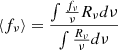 (A.1)
(A.1)
where Rν is the filter transmission function and fν is the flux density in frequency space. When we have estimated the average flux density for both the LyC filter and the UV filter, obtaining ℛobs/ℛint is just a matter of dividing the two.
The template for the intrinsic mock spectra is the Binary Population and Spectra Synthesis (BPASS) model (Eldridge et al. 2017) that was fitted to the composite spectra of the real galaxy sample (see Sect. 3.2 and Begley et al. 2022). The observed spectrum is obtained by redshifting the intrinsic spectrum and modifying the flux to account for the imposed escape fraction, dust attenuation and the optical depth of the IGM and CGM.
The full procedure for simulating the observed spectrum from the intrinsic BPASS model and measuring the corresponding ℛobs is detailed below:
-
We convert the units from L⊙/Å (units of the template spectrum, luminosity density in wavelength space) to μJy=erg/s/cm2/Hz (flux density in frequency space) and redshift the spectrum according to the input parameter, z.
-
Fluxes at wavelengths below the Lyman limit (912Å) are reduced by multiplying with the given escape fraction, fesc.
-
We apply dust attenuation at wavelengths above the Lyman limit using the Reddy et al. (2016b) dust curve and the input value for the attenuation in the V-band, AV.
-
We compute the flux ratio using the definition of ℛobs in Eq. 1, where the average flux density per unit frequency is obtained with Eq. A.1.
-
We multiply the flux ratio from step (4) according to the integrated LyC transmission (
 ).
). -
To account for the intrinsic flux ratio, we multiply the ratio from step (5) with the sampled input ℛint divided by the intrinsic flux ratio of the original BPASS spectrum.
-
Finally, we sample an error on ℛobs from a normal distribution with standard deviation given by the input σR and add it to the reported ℛobs value.
All Tables
All Figures
|
Fig. 1. Illustration of a mock spectrum with the U-band (LyC) and V606 (non-ionising UV) filters marked by the shaded areas. The Lyman limit is indicated with the vertical dashed black line. The fundamental observable, the LyC–to–non-ionising–UV flux ratio, ℛobs (see Sect. 2.2) measures the flux captured by the U-band (left) divided by the flux captured by the V606 filter (right). To ensure that the U-filter is always capturing flux short-ward of the Lyman limit, and is thus measuring ionising photons, we imposed a lower redshift bound of z = 3.35 on the galaxy sample. This mock spectrum was obtained from the intrinsic BPASS spectrum that was fitted to the stacked VANDELS spectrum in Begley et al. (2022) (see Sect. 3.2). The flux below the Lyman limit was attenuated according to an assumed fesc = 20%, whilst dust attenuation was applied to the non-ionising region using the Reddy et al. (2016b) dust curve and a value of AUV = 2.3. The full spectrum was multiplied with a simulated IGM transmission (exhibiting a transmitted fraction of 14% through the U filter; see Sect. 3.3). |
| In the text | |
|
Fig. 2. Distribution of the observed LyC–to–non-ionising–UV flux ratio, ℛobs, exhibited by our final sample of 148 star-forming galaxies (see Sect. 2). The dashed line marks the median observed flux ratio of the sample. This distribution constitutes the observed data in our Bayesian inference framework (see Sect. 4), and thus provides the fundamental observational constraint on estimates relating to the escape fraction. The figure was adapted from Begley et al. (2022). |
| In the text | |
|
Fig. 3. Graphical representation of the two levels in the hierarchical Bayesian inference framework. The method of inference for individual galaxy parameters (see Sect. 4.1) is contained within the main box (denoted Galaxy i), while the full figure includes the hierarchical extension to the Bayesian network incorporating the population parameters (see Sect. 4.2). The grey outlines of multiple boxes in the background indicate the conditional independence between individual galaxy observations. The filled squares denote free sampled parameters, while the rectangle with a solid border denotes a deterministic node (the value is unambiguously determined from the input parameters and Eq. 2). The rectangle with the dashed border denotes a probability distribution with which the likelihood of the observed data, denoted with a circle, is evaluated. The observational error on ℛobs, σℛ is a fixed input to the model. |
| In the text | |
|
Fig. 4. Four physically motivated distributions of the escape fraction placed on a scale to indicate their connection to the two simplified physical pictures of how ionising photons may escape the ISM of their host galaxy. The blue picture represents the density-bounded leakage mechanisms, while the green scenario is where ionising photons escape through ionised low-density channels. In both scenarios the arrows indicate the escape of LyC photons. The constant distribution represents a scenario where all galaxies have the same physical conditions, and LyC photons escape via purely density-bounded leakage from Strömgren spheres with the same column density, while the bimodal model can represent an ionisation-bounded scenario where leakage is mostly strongly sightline dependent and/or a density-bounded scenario that is strongly time variable. The log-normal and exponential distribution represent complex mixtures of the two main leakage mechanisms. |
| In the text | |
|
Fig. 5. Corner plot showing the 1D and 2D marginalised posteriors for the escape fraction, fesc; the integrated transmission through the U-band filter, |
| In the text | |
|
Fig. 6. 1D and 2D marginal posterior distributions of the set of population parameters, ϕ, for each of the four models described in Sect. 4.3. The dashed lines indicate the mode of the posterior samples, and values are reported as the mode with the 68 per cent HDP interval. Panel (a): 1D marginal posterior of the population parameter ϕconst = μ (blue), describing the constant escape fraction value most likely to describe all galaxies in the sample. Panel (b): Corner plot showing the 1D and 2D marginal posterior distributions of the set of population parameters ϕlognorm (pink), describing a log-normal distribution of escape fractions. Here μ and σ represent, respectively, the mean and standard deviation of the natural logarithm of the escape fraction. Panel (c): 1D marginal posterior of the population parameter ϕexp = μ (orange), which represents the scale parameter in an exponential distribution of escape fractions. Panel (d): Corner plot containing the 1D and 2D marginal posteriors for the set of population parameters ϕbimodal (green), which describes a bimodal distribution of escape fractions: w denotes the fraction of galaxies with a constant escape fraction equal to zero, while μ and σ describe the escape fraction of the remaining galaxies as being normally distributed. |
| In the text | |
|
Fig. 7. Median cumulative distribution of the population distribution of escape fractions for each of the four models. For each model we (i) selected 10 000 parameter sets from the chains of posterior samples displayed in Fig. 6, (ii) evaluated the CDF of the distribution given by the selected population parameters on a grid of escape fractions, and (iii) computed the median of the 10 000 corresponding CDF values for each index of the escape fraction grid. The median is shown as a solid line, while the shaded region marks the 16th and 84th percentile intervals. For reference, we plot the CDF of a uniform distribution as a dashed line. |
| In the text | |
|
Fig. 8. Posterior predictive test of the four models. (Top) Visual illustration of the KS score, which measures the maximum difference between the eCDF of the observed flux ratios, ℛobs (plotted in black), and the eCDF of a simulated ℛobs distribution dependent on respectively the constant, log-normal, exponential, and bimodal model distribution of the escape fraction as inferred from the Bayesian framework. (Bottom) Residual (the model eCDF minus the data eCDF). |
| In the text | |
|
Fig. 9. Cumulative distribution of the escape fraction as parametrised by the exponential scale parameter, ϕexp = μ, inferred for, respectively, the full sample (grey), the galaxy subsample with lowest UV slopes (blue), and the subsample with highest UV slopes (red). The inset shows the corresponding inferred posterior distribution, where the dashed line marks the mode of the distribution. |
| In the text | |
|
Fig. 10. Cumulative distribution of the population distribution of the escape fraction. Shown are the median CDF for the exponential model inferred in this work (in orange; the shaded region marks the 16th and 84th percentile interval) and the eCDF for a selection of SPHINX galaxies (in black) with somewhat similar properties to our observed sample. For context, the CDF for selections of red high-mass galaxies and blue low-mass galaxies in SPHINX are plotted. All selections are described in Sect. 6.2. |
| In the text | |
Current usage metrics show cumulative count of Article Views (full-text article views including HTML views, PDF and ePub downloads, according to the available data) and Abstracts Views on Vision4Press platform.
Data correspond to usage on the plateform after 2015. The current usage metrics is available 48-96 hours after online publication and is updated daily on week days.
Initial download of the metrics may take a while.