| Issue |
A&A
Volume 695, March 2025
|
|
|---|---|---|
| Article Number | A32 | |
| Number of page(s) | 15 | |
| Section | Astrophysical processes | |
| DOI | https://doi.org/10.1051/0004-6361/202449997 | |
| Published online | 03 March 2025 | |
Physically motivated modelling of LyC escape fraction during reionisation
1
Max-Planck-Institut für Astrophysik, Karl-Schwarzschild-Str. 1, 85741 Garching, Germany
2
Scuola Normale Superiore, Piazza dei Cavalieri 7 I-50126 Pisa, Italy
⋆ Corresponding author; This email address is being protected from spambots. You need JavaScript enabled to view it.
Received:
15
March
2024
Accepted:
10
December
2024
Abstract
Aims. We present an analysis of the Lyman continuum (LyC) escape fraction of high-redshift galaxies using an analytic post-processing approach.
Methods. We applied the model to ∼6 × 10⁵ galaxies of the Illustris TNG50 simulation in the redshift range z = 5.2 − 20.
Results. Our study reveals a bimodal nature of LyC escape that is associated with either (a) high-metallicity (10−3.5 < Z < 10−2) low-mass (M⋆ < 107 M⊙) galaxies, which due to their efficient cooling exhibit extended star formation, with photons escaping primarily from the outer regions of the galactic plane (ext-mode), or (b) low-metallicity (Z < 10−3) moderately massive galaxies (M⋆ < 108 M⊙) in which star formation can only take place in small high-density regions, with localised LyC escape originating from these regions (loc-mode). While the loc-mode is present at all redshifts under investigation, the ext-mode becomes prominent in small galaxies at later cosmic times, that is, once sufficient metal enrichment has occurred. Building on these findings, we have developed an analytical fitting formula to determine the escape fraction of galaxies based on their stellar and gas mass as well as redshift, providing a valuable subgrid modelling tool for future studies.
Key words: radiation mechanisms: non-thermal / galaxies: high-redshift / dark ages, reionization / first stars
© The Authors 2025
 Open Access article, published by EDP Sciences, under the terms of the Creative Commons Attribution License (https://creativecommons.org/licenses/by/4.0), which permits unrestricted use, distribution, and reproduction in any medium, provided the original work is properly cited.
This article is published in open access under the Subscribe to Open model.
Open Access funding provided by Max Planck Society.
1. Introduction
The escape of Lyman continuum (LyC) photons, primarily emitted by young massive stars residing in galaxies, is a critical process driving the reionisation of the Universe (see Dayal & Ferrara 2018 for a comprehensive review). To understand the history and structure of this cosmic event, it is crucial to gain insights into the LyC escape fraction. Indeed, by quantifying the fraction of LyC photons that successfully escape from galaxies and understanding the underlying physical mechanisms that facilitate or hinder this escape, one can obtain valuable information about the sources, mechanisms, and conditions contributing to the reionisation process.
Due to the attenuation caused by neutral gas, the direct observation of LyC escape is limited to low redshifts, where typical escape fractions of ≲0.05 have been measured (e.g. Vanzella et al. 2010; Nestor et al. 2011; Boutsia et al. 2011; Mostardi et al. 2013; Grazian et al. 2016; Matthee et al. 2016; Alavi et al. 2020; Pahl et al. 2021). These values are insufficient to meet the current constraints on the timing of reionisation. However, some authors (e.g. Inoue et al. 2006) have suggested that in the redshift range 1 ≤ z ≤ 4, the escape fraction increases with redshift, indicating that during the epoch of reionisation, LyC escape might have been significantly higher.
To investigate LyC escape at higher redshifts, indirect indicators are employed, such as the ratio of the [OIII]5007 Å/[OII]3727 Å lines (e.g. Nakajima & Ouchi 2014; Tang et al. 2021). High values of this ratio suggest that galaxies are density (rather than ionisation) bound; that is, they are more likely to be LyC leakers. Additional metal lines, such as MgII (e.g. Chisholm et al. 2020; Xu et al. 2016), CII (e.g. Heckman et al. 2001; Leitet et al. 2011), and SiII and SiIII (e.g. Jones et al. 2013; Chisholm et al. 2017), can also be utilised to study the presence of neutral and ionised regions, providing further insights into the occurrence of LyC escape. Ly-α equivalent width (e.g. Dijkstra et al. 2014) and line separations (e.g. Verhamme et al. 2015) have also been employed as indicators of LyC escape. Indeed, a larger equivalent width indicates a higher rate of LyC production within the galaxy, as the Ly-α line primarily arises from hydrogen recombination. On the other hand, line separations are created by the scattering of Ly-α photons in neutral gas such that a smaller line separation indicates lower amounts of intervening neutral gas and, consequently, a larger LyC escape fraction. Finally, it has been observed that the slope of the non-ionising UV spectrum exhibits a strong correlation with LyC escape (Chisholm et al. 2022), with a redder UV slope indicating stronger dust attenuation (i.e. a significant absorption of LyC radiation). Therefore, galaxies with steeper UV slopes tend to have lower LyC escape fractions.
Theoretical investigations have endeavored to model the escape of LyC radiation from galaxies. These studies employ methodologies such as Monte Carlo radiation transfer (MCRT) in post-processing (e.g. Paardekooper et al. 2015; Ma et al. 2016, 2020; Kostyuk et al. 2023) and hydrodynamic radiation transfer (RT) simulations (e.g. Kimm & Cen 2014; Ocvirk et al. 2016, 2021; Rosdahl et al. 2018, 2022; Lewis et al. 2020; Yeh et al. 2023). However, determining the escape fraction poses challenges due to degeneracies between star formation efficiency and escape fraction, as well as the large dynamic range involved, requiring additional assumptions about the subgrid configuration. As a consequence, various studies have reported average values of the escape fraction that can vary up two orders of magnitude. This is in addition to finding different dependencies of the escape fraction on galactic properties, such as stellar and gas mass, although most studies agree that the escape fraction decreases with increasing mass for the highest stellar masses.
An alternative approach to understanding LyC escape is currently being developed by Ferrara et al. (in prep., F24). This involves constructing an analytic model that can identify LyC leakage from a galaxy based on a few simple assumptions. The model represents the galaxy as a thin slab with dusty gas surrounding the galactic plane acting as the absorber of LyC radiation. With these assumptions, the model aims to provide insight into the mechanisms and conditions governing LyC escape, offering a streamlined framework for studying this phenomenon in galaxies. Due to the analytical nature of the model and the broad spectrum of physical scales involved in LyC escape, the objective is not to determine precise values for the escape fraction but rather to acquire a qualitative insight into the physical characteristics of galaxies that leak LyC radiation. In this study, we employ the aforementioned physical model to investigate the characteristics of LyC radiation in galaxies from the TNG50 cosmological simulation. The aim of this work is to provide an introduction into the capabilities of a simplified semianalytic model to capture qualitative behaviour of LyC escape at high redshifts. We aim to further expand the complexity and reliability of the model in future works.
We have structured this work as follows: In Sect. 2, we present our methodology for modelling LyC photon production and escape in TNG50 galaxies. In Sect. 3, we discuss the geometry of LyC escape as well as its correlation with galactic properties. We subsequently introduce a fitting formula for the LyC escape fraction and analyse its accuracy in Sect. 4. Finally, we summarise our results and conclude in Sect. 5.
2. Method
Here we present our approach for calculating the LyC escape fraction of TNG50 galaxies using the semianalytic model developed in F23. We first introduce the TNG simulations, followed by a description of the physically motivated model adopted to evaluate the escape fraction, and finally, we present its application to galaxies extracted from TNG50.
2.1. The IllustrisTNG simulation
In this work we model the LyC escape fractions of galaxies taken from the Illustris TNG50 simulation (Pillepich et al. 2018b; Springel et al. 2018; Naiman et al. 2018; Nelson et al. 2018; Marinacci et al. 2018), which is one of three large-scale cosmological simulations, together with TNG100 and TNG300, sharing the same physical modelling. TNG50 simulates the evolution of structures in a cosmological volume of (51.7 cMpc)3 (Nelson et al. 2019; Pillepich et al. 2019). The initial conditions were generated with the N-GenIC code (Springel et al. 2005) at z = 127, adopting cosmological parameters consistent with the measurements by the Planck satellite (Planck Collaboration I 2016), that is Ωm = 0.3089, Ωb = 0.0486, ΩΛ = 0.6911, h = 0.6774, σ8 = 0.8159 and ns = 0.9667. The simulation evolves down to z = 0, and the properties of galaxies are validated against observational data, providing confidence that the high-redshift galaxies analysed in this study are realistic progenitors of the galaxy populations observed today.
The underlying physical model utilised in this study is implemented using the AREPO code (Springel 2010), which employs the equations of ideal magnetohydrodynamics to simulate the interaction of baryonic matter. The simulation is performed on a Voronoi grid, enabling a detailed representation of the spatial distribution and properties of the simulated system. The galaxy formation model employed in this work builds upon the framework developed by Weinberger et al. (2017) and Pillepich et al. (2018a). In this model, the gas particles contained within Voronoi cells with a hydrogen number density nH > 0.1 cm−3, determined based on the Kennicutt–Schmidt relation (Springel & Hernquist 2003), are stochastically converted into individual stellar particles. Each stellar particle represents a distinct stellar population and follows a Chabrier initial mass function (IMF; Chabrier 2003). To account for subgrid processes and the role of pressure support in star forming gas, the Springel & Hernquist (2003) model for the interstellar medium (ISM) is incorporated. Feedback from supernovae is modelled through the implementation of decoupled kinetic wind particles (Pillepich et al. 2018a).
The initial dark matter and gas particles mass is 4.5 × 10⁵ M⊙ and 8.5 × 10⁴ M⊙, respectively. However, the refinement and de-refinement of Voronoi cells leads to variation of these values within a factor of two. The spatial resolution varies strongly from the inner part of the galaxies to the IGM. The mean size of star forming gas cells, which are of most relevance for our study, is 144 physical parsecs at z = 6, with 16–84th percentiles ranging from 96 to 184 ppc. Whenever a stellar particle is formed, it inherits the mass of the baryonic gas cells it formed in, and its mass decreases as the stellar population evolves with time.
The galaxies we investigate in this study are identified as TNG50 subhalos. These are found using the SubFind algorithm (Springel et al. 2001), which employs the friends-of-friends approach (Davis et al. 1985) to detect distinct structures within the simulation. Subhalos are defined based on a minimum particle threshold, with a minimum subhalo mass of approximately 106 M⊙. At the centre of galaxies surpassing a mass threshold of 1010.8 M⊙, black hole (BH) seeds with an initial mass of 8 × 10⁵ h−1 M⊙ are positioned. The growth of the seeds occurs through either BH–BH mergers or gas accretion, following the Bondi formalism with the Eddington rate setting the accretion limit. To account for the feedback effects of black holes, the simulation incorporates various mechanisms such as thermal heating, radiative influences, and kinetic wind (Weinberger et al. 2017). Moreover, the simulation tracks the metal enrichment process, including the individual abundances of elements such as C, N, O, Ne, Mg, Si, Fe, and Eu, in addition to modelling the content of H and He gas. While radiation transfer is not modelled explicitly, a spatially uniform UV-background (UVB; from Faucher-Giguère et al. 2009) is turned on at z < 6.
2.2. Physical model of LyC escape
The model underlying our calculations of the escape fraction was developed in F23. Here, the galaxy is considered a plane parallel slab (as in Ferrara et al. 2019), with stars populating the galactic plane, while the gas is distributed above and below it with a constant density up to a scale height of H, resulting in a column density N0. This is a simplification of the typically more complex geometry of the gas distribution. However, it is a reasonable approximation given a gas distribution that is concentrated around the immediate surrounding of the source with only a few cells significantly contributing to gas absorption. A more realistic picture would involve the resolution of the two-state ISM which is not included in the TNG50 model.
LyC photons emitted by stars are absorbed by both gas and dust, and they can escape the galaxy if the ionising flux is large enough to form an ionised channel in the gas. Although lower mass galaxies at high redshift typically lack a disc-like structure, the fundamental physical assumption underpinning this model is that the scale height of the star forming region is notably smaller than the height of the gas distribution. This assumption is further examined in Appendix B, where we show that statistically it holds over the full range of galactic masses we examined.
We defined the ionising photon flux Fi (in units of cm−2 s−1) as
 (1)
(1)
where ν is the frequency, νL = 3.2 × 10¹⁵ Hz is the frequency corresponding to the H ionisation threshold 13.6 eV, F(ν) is the ionising energy flux, and hP is the Planck constant.
As in Ferrara et al. (2019), the ionising energy flux is expressed through a power law:
 (2)
(2)
where FL is the energy flux at νL, while β is usually assumed to be in the range 4 − 5 for PopII stellar populations (Leitherer et al. 1999). In this work we use β = 4. Therefore, Eq. (1) becomes Fi = FL/(βhP). Here, we obtain FL through its connection to the SFR. For this purpose, we use the conversion between UV luminosity F1500 and the surface density of star formation ΣSFR employed by the REBELS collaboration (Dayal et al. 2022), that is F1500 = ΣSFRκ−1. For a Chabrier IMF, κ = 7.1 × 10⁻²⁹ M⊙ yr−1 erg−1 s Hz and F1500 ≈ FL. Hence, the ionising flux can be calculated as
 (3)
(3)
Given the gas density, the photon flux can be related to the photon-to-gas density ratio U through U = Fi/nc, with c being the speed of light. We can further relate the flux to the Strömgren depth lS (i.e. the maximum distance that can be ionised by the flux) through lS = Fi/(n2αB), with αB being case B recombination parameter. We could then define the maximum column density that can be ionised by the flux,
 (4)
(4)
and the optical depth encountered by LyC photons through the hydrogen gas,
 (5)
(5)
The ionising flux is additionally absorbed by the dust content in the gas, which has an optical depth to LyC photons of
 (6)
(6)
Here, AL/AV = 4.83 is the LyC to V-band attenuation ratio assuming a visual extinction to reddening ratio of RV = 3.11, and σd, V = 4.8 × 10⁻²²𝒟 cm2 is the dust cross-section per H atom in the V-band (Weingartner & Draine 2001). Assuming a linear relation between metallicity Z and dust, the dust-to-gas ratio normalised to the galactic value 𝒟 can be written as 𝒟 = Z/Z⊙, with Z⊙ = 0.0134 being the solar metallicity (Asplund et al. 2009).
We could thus determine the gas column density at which the dust optical depth reaches unity as
 (7)
(7)
This simplifies Eq. (6) to τd = N0/Nd.
The LyC escape fraction is defined as the fraction of photons not absorbed by the optical depth, that is, fesc = e−τtot, where τtot = τHI + τd is the total optical depth of the gas in the galaxy. Hence, we can write the escape fraction as2
![Mathematical equation: $$ \begin{aligned} f_{\rm esc} = \exp \left[-N_0\left(\frac{1}{N_{\rm S}}+ \frac{1}{N_{\rm d}} \right) \right]. \end{aligned} $$](/articles/aa/full_html/2025/03/aa49997-24/aa49997-24-eq8.gif) (8)
(8)
2.3. Escape fraction of TNG50 galaxies
In this work, we analysed the escape fraction of ≈600 000 galaxies extracted from 17 TNG50 snapshots in the redshift range 5.2 ≤ z ≤ 20. To ensure sufficient resolution, we post-processed only galaxies with a minimum stellar and gas mass of 105.5 M⊙ and 106 M⊙, respectively, located within twice their stellar half mass radius. This ensures that the smallest galaxies are resolved with more than 10 gas particles. This results in 77 498 galaxies at z = 5.2 and only 6 at z = 20 (see Fig. 1 top). As the TNG50 snapshots are not equally spaced in redshift and a much larger number of galaxies have formed at later times, the lower redshift range is sampled with significantly more galaxies. Additionally, given their much larger abundance the sample is highly biased towards low-mass galaxies. We sample a factor of 104 more galaxies with M⋆ ≈ 106 M⊙ as compared to galaxies with M⋆ ≈ 1010 M⊙ (see Fig. 1 bottom).
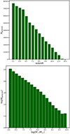 |
Fig. 1. Number of galaxies processed as a function of redshift (top) and as a function of stellar mass (bottom). |
To obtain the LyC escape fraction for each galaxy we proceeded as follows. First, we defined the galactic plane as the surface spanned by the first two principle axes of the galaxy. Then, we cut out a box with a side length of four times the stellar half mass radius, rHMR. The gas particles contained in that box were distributed on a regular Cartesian grid with 1003 cells (see Appendix A for a convergence study), ensuring that both the gas distribution and the star forming regions are well resolved. We defined the gas scale height, H, as the height above and below the galactic plane, containing ≈63% (1/e) of the gas mass.
We then projected quantities relevant to the calculation of the escape fraction onto the galactic plane. More specifically, the gas mass per unit area in each 2D grid cell {i, j} is given by
 (9)
(9)
with mgas, ijk being the gas mass contained in a given grid cell, and Acell area of the cell. ΣSFRi, j was calculated in the same way, by substituting mgas, ijk with the instantaneous SFR in each cell SFRijk. Σmi, j can then be related to the gas column density in the cell through N0, ij = Σmi, j/2μ, with μ being the mean molecular mass assumed to be the mass of a hydrogen atom in our simplified model, and the factor 2 accounts for the symmetry of the gas distribution below and above the galaxy. Finally, the metallicity of a grid cell Zi, j is given by the mass weighted mean in a given column:
 (10)
(10)
This value can be related to the value of Nd in that cell through Eq. (7).
To obtain the escape fraction from a cell, we compute N0, NS and Nd individually for each element of the 2D grid and evaluate fesc, cell using Eq. (8). The escape fraction of the galaxy, fesc, is then given by
 (11)
(11)
with Fi, cell being the ionising flux in each grid cell obtained using Eq. (3) with ΣSFRi, j.
It should be noted that neither the analytic method for the calculation of the escape fraction nor the hydrodynamic model used to simulate star formation are fully taking into account the multi-phase structure of the ISM. While we anticipate that an improved subgrid modelling of the complex nature of the ISM would lead to quantitative differences in some of our results, we remain confident that the qualitative conclusions will remain unchanged. This is supported by the study conducted in Kostyuk et al. (2023), where we demonstrated that the inclusion of a subgrid escape fraction, while affecting the absolute value of fesc, did not alter its dependence on galactic properties. Furthermore, we also note that, as of now, no hydrodynamical simulation is able to cover all the relevant scales involved, that is all studies of escape fraction are necessarily resolution limited.
3. Results
3.1. Dependence on stellar mass and redshift
In Fig. 2 we investigate how the LyC escape evolves as a function of the galactic stellar and gas mass. For this purpose, we classified galaxies based on their redshift, as well as their stellar and gas mass. We represent the averaged escape fraction ⟨fesc⟩ of galaxies within each specific bin using a colour scale. We observe a strong correlation between stellar mass and the average escape fraction, with ⟨fesc⟩ steadily increasing with M⋆ up to M⋆ ≈ 106.5 M⊙ (107 M⊙) for z = 5.2 (10). Beyond that, ⟨fesc⟩ decreases and becomes essentially zero for M⋆ > 108 M⊙. As redshift increases, the peak of the escape fraction shifts towards higher stellar masses. This phenomenon is more clearly discernible in Fig. 3, which is discussed later.
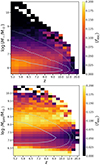 |
Fig. 2. Average LyC escape fraction of all galaxies in a given bin (colour scale) as a function of redshift and galactic stellar mass (top) as well as gas mass (bottom). The white contours denote the 1 (solid), 2 (dashed) and 3 (dotted) sigma distribution of galaxy counts. |
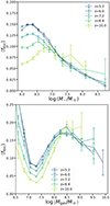 |
Fig. 3. Average LyC escape fraction as a function of stellar mass (top) and gas mass (bottom) for a sample of redshifts. The error bars denote the statistical error of the mean. |
A larger scatter is observed in the dependence of the escape fraction on the galactic gas mass, which emerges as a result of the gas mass exhibiting a weaker correlation (in comparison to the stellar mass) with the metallicity. A higher metallicity results in an increase in dust content and hence absorption as well as in more efficient cooling and thus denser gas, with both factors being strongly anti-correlated with the escape fraction, as is further discussed in Fig. 8. The generally higher ⟨fesc⟩ as compared to the top panel, is explained by the majority of the high-escape bins being located outside of the regions containing most of the galaxies so that the bins are typically sampled with fewer galaxies. We observe that the escape fraction exhibits one maximum at Mgas = 108 M⊙ at z = 5.2, which increases with redshift as in the top panel, reaching Mgas = 108.5 M⊙ at z = 10. A second peak observed for galaxies with Mgas < 106.5 M⊙, shows instead an opposite redshift evolution. This peak can be attributed to a secondary mode of LyC escape correlated to extensive star formation regions and elevated metallicity levels. We thoroughly investigate this phenomenon in Fig. 4.
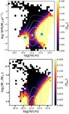 |
Fig. 4. Average escape fraction as a function of scale height and SFR (top) as well as a function of scale height and galactic stellar mass (bottom). The contours represent the distribution of galaxies as described in Fig. 2. The numbers label the areas that we identified as the localised escape mode (loc-mode, number 1), the extended escape mode (ext-mode, number 2) and the LyC dark mode (number 3). |
In Fig. 3 we show the averaged escape fraction as a function of stellar and gas mass for a sample of redshifts. Here we see more clearly how the peak of ⟨fesc⟩ shifts towards higher stellar masses with increasing redshift, while at the same time its value decreases. For M⋆ ≥ 107 M⊙, though, fesc converges to similar values at all redshifts. It should be noted that the high redshift results are less reliable due to the smaller sample of galaxies (see Fig. 1).
As already seen in Fig. 2, the escape fraction decreases with increasing gas mass, reaching a minimum at Mgas ≈ 107.3 M⊙ before increasing again for higher gas masses. We note that this initial decrease is particularly strong for lower redshifts, reflecting the trend in Fig. 2. Additionally, the lower panel shows a smaller difference in the amplitude of the peak across the different redshifts. The increase in the escape fraction of galaxies with the smallest gas masses is likely to reflect the population of galaxies that have some star formation but almost no gas obscuration.
3.2. Escape modes
Next, we investigate the correlation of fesc with various galactic properties. To do this, we analyze how these properties interplay to shape the conditions that enable or inhibit the escape of ionizing radiation.
Initially, we examine the impact of gas distribution within the galaxy on the escape of LyC radiation. To accomplish this, in Fig. 4 we show the average escape fraction as a function of scale height and the star formation rate (SFR) as well as the scale height and galactic stellar mass, which serves as a measure of how closely the gas is distributed in relation to the galactic plane. We observe the presence of two distinct modes, denoted as localised escape mode (loc-mode, corresponding to the area labelled with the number 1 in the top plot) and the extended escape mode (ext-mode, number 2), both exhibiting ⟨fesc⟩> 0.23. The loc-mode is characterised by higher scale heights (H > 1021 cm) and a wider range in SFR. The ext-mode, on the other hand, exhibits smaller scale heights (H < 1021 cm), and is limited to relatively low SFRs. The two regions are separated by a region with small LyC escape (number 3), which we refer to as the LyC dark mode, where the average escape fraction is lower. This mode encompasses the majority of galaxies, as evidenced by the contour lines. In the lower plot we see that the two mode structure of the escape fraction can also be identified as a function of stellar mass. However unlike with SFR there is no lower stellar mass bound for the escape mode.
In Fig. 5 we investigate the contributions of these two modes to the density of ionising photon escape at various redshifts. We see that the ext-mode dominates the LyC escape for low-mass galaxies M⋆ ≈ 106 M⊙ while in all other mass bins the loc-mode is the dominant one. As small galaxies dominate the galactic population at high redshifts LyC leakage via ext-mode contributes a comparable amount to the escaping ionising photon budget as the loc-mode at early times(see right-hand plot). However, at lower redshifts the ext-mode quickly becomes subdominant contributing only ≈20% of the ionising photons at z = 5.5.
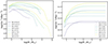 |
Fig. 5. Comparison of the escape density of the ionising photons from the loc-mode (solid) and ext-mode (dashed) as a function of stellar mass (left) and well as the cumulative escape (right). |
In Fig. 6 we showcase a selection of three galaxies from each of the three regions marked in Fig. 4, by looking at the distribution of their escape fractions, their ionising fluxes, Fi, and the gas optical depth τHI, where the latter is approximately equivalent to the optical depth τtot, as in these cases Nd is negligible4.
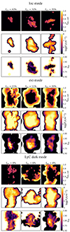 |
Fig. 6. Projected maps of the escape fraction; ionising flux, Fi; and the gas optical depth, τHI, distribution from individual grid cells (box size 4 stellar half mass radii) for three example galaxies from the loc-mode (top panels), ext-mode (centre), and LyC dark mode (bottom). |
Galaxies belonging to the loc-mode exhibit relatively small localised escape regions, often situated in proximity to the centre of the galaxy. Thus the earlier adopted name for said mode. In contrast, galaxies belonging to region 2 display large escape fractions over an extended area at the outskirts of the galaxies, with no LyC escaping from the inner regions. Finally, galaxies from the LyC dark mode display characteristics from both escape modes, but generally exhibit lower average escape fractions.
The loc-mode reveals concentrated regions of ionising flux, primarily found in the central areas of galaxies where the star formation process takes place. This results in the distinct compact escape channels. The abundance of ionising photons in these regions leads to a low τHI within the central areas of the galaxy. Consequently, the correlation between escape fraction and scale heights becomes apparent: as the density is inversely proportional to the scale height (n ∝ H−1), and the recombination rate increases ∝n2, it follows that the escape fraction increases with increasing scale heights and hence less dense gas.
In contrast, galaxies in the ext-mode exhibit a considerably larger area that emits ionising flux. However, when analysing τHI, a noteworthy pattern emerges: the central region displays an inverse correlation between Fi and LyC escape, akin to what is observed in the loc-mode. Specifically, the central region exhibits the highest τHI ratio, while the outskirts display minimal absorption. Consequently, in order for escape fractions to be substantial, it becomes crucial for a significant portion of star formation to occur in the outer regions of the galaxy. In this mode, the correlation with small-scale height stems from star formation being driven by higher densities in the outer regions of the galaxy. Despite the recombination rate being larger in these higher density regions, it is compensated by the elevated production rate of ionising photons driven by star formation. The interplay between star formation and gas absorption yields the distinct escape rings observed in galaxies sampled from the ext-mode. These escape rings are a manifestation of the relative importance of star formation and gas absorption in shaping the escape characteristics of these galaxies.
Finally, galaxies from the boundary region exhibit properties that are observed in both the aforementioned escape modes. However, this regime presents limitations for escape from the centre due to small-scale height, as well as a scarcity of star formation in the outer regions of the galaxy. These factors collectively restrict escape through both channels, as illustrated in the lower panels of Fig. 6. The areas emitting ionising flux in galaxies from the boundary region are less extended compared to the example galaxies from the ext-mode. Additionally, there is a weaker correlation between low τHI and high star formation regions. In summary, galaxies in the LyC dark mode show star formation characteristic of both escape modes, yet they lack the necessary conditions to facilitate LyC escape through either of these modes.
To verify the universality of the escape modes observed in our sample, we analysed the LyC escape characteristics within each galaxy. To quantify the degree of localisation of the LyC escape in a given galaxy, we employed the Gini coefficient, which we calculated as
 (12)
(12)
with N being the total number of grid cells in a given galaxy map and ycell := fesc, cellFion, cell as the ionising flux weighted escape fraction of each cell and icell being the index of a grid’s cells ordered by their ycell values. A Gini value of one signifies that all ionising radiation within a galaxy is concentrated in just one cell, resulting in a highly localised escape. On the other hand, a Gini value of zero indicates that the ionising photons leak equally from all cells, indicating a more evenly distributed escape pattern.
For galaxies exhibiting fesc > 0.1 and a scale height H < 1020.8 cm (corresponding to the ext-mode), the average Gini coefficient is  . In contrast, galaxies with fesc > 0.1 and a scale height H > 1021.3 cm (corresponding to the loc-mode) exhibit a higher average Gini coefficient of
  . These findings clearly indicate a notable disparity in the LyC escape geometry between the two modes, and confirm our more qualitative previous discussion.
In Fig. 4 we noticed that in the loc-mode for log(SFR)< − 2.5 the escape fraction is positively correlated to the SFR. However, for log(SFR)> − 2 the trend is reversed. To understand this, in Fig. 7 we examine in more detail galaxies selected on the basis of their SFR. In particular, we select three sample galaxies with high (i.e. log(SFR)> 0), and low (i.e. log(SFR)< − 4) SFR respectively, to explore the physical properties dominating the escape fraction in these regimes. In galaxies with high SFR, the determining factor for the escape fraction in the central region is the dust optical depth τd, which remains unaffected by the ionising flux. However, τd exhibits a correlation with the metallicity. Indeed, a higher metallicity content promotes gas cooling, resulting in an increase in SFR and subsequently leading to a decrease in the average escape fraction ⟨fesc⟩ with SFR. It should be noted, however, that as no dust destruction is present in our model, dust absorption should be regarded as an upper limit. It is worth mentioning that galaxies at the upper limit in the loc-mode showcase substantial LyC escape in the outer regions. Nevertheless, despite the extensive nature of these escape regions, only a small portion of the galaxies’ ionising photons are generated there, ultimately resulting in relatively low overall escape fractions. Conversely, in the low SFR sample (bottom), we observe the presence of only a few small escape channels. In this scenario, the impact of dust absorption is negligible, while the LyC absorption is primarily influenced by the gas optical depth τHI. The escape fraction is thus strongly dependent on the number of ionising photons generated, as τHI is related to the ionising flux (see Eq. (4)), and consequently the SFR.
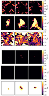 |
Fig. 7. Galaxies with scale heights H > 1021.3 cm selected for their high and low SFR, that is log(SFR/M⊙ yr−1)=0.14, 0.20, and 0.40 (top) and log(SFR/M⊙ yr−1)= − 4.34, −4.05, and −4.08 (bottom figure). From top to bottom, the panels in each figure refer to the cell escape fraction, fesc, cell; optical depth of dust, τd; and of gas, τHI. |
Finally, in Fig. 8 we explore the correlation of the two escape modes with other galactic properties. For this purpose we separated the sample of galaxies into two groups: one with log(H/cm)> 21.3 containing the loc-mode, and one with log(H/cm)< 20.8 containing the ext-mode. We then examine the correlation of these groups separately in relation to various galactic properties. From the top panels we see that there is a significant difference between the two groups with respect to dependencies on galactic gas mass and metallicity.
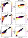 |
Fig. 8. Average escape fraction as a function of metallicity and galactic gas mass (top panels), metallicity and galactic stellar mass (centre), and SFR and stellar mass (bottom). The left and right columns refer to galaxies with log(H/cm)< 20.8 and log(H/cm)> 21.3, which include the ext- and loc-modes, respectively. The contours denote the 1 (solid), 2 (dashed) and 3 (dotted) sigma distribution of galaxy counts. |
For small-scale heights (ext-mode), ⟨fesc⟩ does not significantly depend on the metallicity, but is highly sensitive to the gas mass. All galaxies with significant escape fractions have 10−4 < Z < 10−2 and Mgas ≲ 107 M⊙. We can thus conclude that the ext-mode is characterised by low gas mass, in addition to small-scale heights and SFR, indicating that the bulk of the galaxies in this mode are limited in their LyC escape by gas absorption τHI.
Finally, within the sample of galaxies with a gas mass of approximately 106.5 M⊙, we observe an evolution of ⟨fesc⟩ in relation to metallicity. For Z < 10−3.5, ⟨fesc⟩ increases with increasing metallicity, as in this regime dust absorption is expected to have minimal impact, while the enhancement of metal line cooling facilitates star formation, thereby contributing to a higher escape fraction. However, for Z > 10−3, this trend reverses due to the growing significance of dust absorption, which outweighs the additional star formation resulting from more efficient cooling.
Within the group encompassing galaxies with large-scale heights (loc-mode), a strong negative correlation between the average escape fraction ⟨fesc⟩ and metallicity becomes evident. Consequently, galaxies with Z > 10−3 exhibit negligible ⟨fesc⟩. This result highlights that the escape of LyC photons in the loc-mode is predominantly limited by dust absorption, as exemplified in the galaxy sample depicted in Fig. 7. Notably, there appears to be no upper limit to fesc based on gas mass, indicating that the additional star formation facilitated by the gas compensates for the heightened gas absorption. Conversely, in the case of galaxies with Mgas ≲ 107.5 M⊙, the escape fraction experiences a decline, which reflects the limited star formation observed in these gas-deficient galaxies.
When investigating the average escape fraction as a function of metallicity and stellar mass instead of gas mass, notable changes occur in the distributions. The primary reason for this is the correlation between stellar mass and metallicity, which consequently correlates with the dust optical depth (τd). For galaxies with small-scale heights (ext-mode), the bins displaying high ⟨fesc⟩ values span a wider region in the M⋆ − Z space. This indicates that dust absorption plays a secondary role in the LyC escape for these galaxies. Nonetheless, the average escape fractions are generally lower compared to the plot above, as galaxies within a specific stellar mass bin exhibit varying gas fractions and thus have a wider spread in τHI. For galaxies with large-scale heights, we observe that those with M⋆ ≳ 108 M⊙ have negligible escape fractions. This results from the high metallicities (Z > 10−3), leading to strong dust absorption and consequently smaller escape fractions.
When examining the distribution of galaxies as a function of stellar mass and SFR, we see that both groups have a similar behaviour. However, the group with small-scale heights (ext-mode) has a slightly higher scatter in SFR at a fixed M⋆. This is likely caused by both old, mostly quenched galaxies with little feedback, as well as efficiently cooling high SFR galaxies with small-scale height. The sequence corresponding to the small-scale heights extends to approximately one order of magnitude higher SFR and M⋆. The reason is that large galaxies are usually found at lower redshifts and are usually more enriched by metals. This facilitates their cooling resulting in lower scale heights.
3.3. Redshift evolution
In Fig. 9 we examine how the dependence of fesc on SFR and scale height discussed in the previous section evolves with redshift. In the top panel we observe that the highest values of ⟨fesc⟩ are found at higher values of SFR with increasing redshift, resembling the dependence on M⋆ depicted in Fig. 2. To understand this trend we note that at higher redshifts galaxies are more metal poor. This means that escape through the localised mode is facilitated, while escape through the extended mode is either unaffected or even hindered when the metallicity is not sufficient to facilitate the extended star formation required. As the ext-mode is only found in galaxies with M⋆ ≲ 107 M⊙, the lack of this escape mode at higher redshifts results in ⟨fesc⟩ peaking at higher stellar masses.
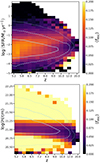 |
Fig. 9. Redshift evolution of the average escape fraction as a function of SFR (upper panel) and scale height (lower). The contours denote the 1 (solid), 2 (dashed) and 3 (dotted) sigma distribution of galaxy counts. |
This behaviour is further supported by the lower plot, where the ⟨fesc⟩ for galaxies with small-scale heights, that is corresponding to the ext-mode, decreases with increasing redshift within the range of 1020.5 cm < H < 1021 cm. Conversely, for galaxies with large-scale heights exhibiting localised LyC escape, ⟨fesc⟩ shows an opposite trend, particularly evident in the range of 1021.1 cm < H < 1021.3 cm. As a result, as seen in Fig. 3, the LyC escape fraction averaged over all galaxies decreases with increasing redshift due to less massive galaxies not leaking photons through the process of the ext-mode. Even though leakage through the loc-mode for massive galaxies is enhanced at high redshifts, their abundance in the early Universe is too low, to compensate for the decrease in the ext-mode leakage.
While this is surprising given the strong observational evidence for a decrease in LyC escape with redshift, our results do not contradict these findings. First, the observed reduction in escape fraction with redshift is mostly seen in the ext-mode, which is predominant in low-mass galaxies. Instead, galaxies identified as LyC leakers have higher stellar masses, likely categorising them into the loc-mode, where we observe an increase in the escape fraction with redshift. Additionally, considering that a UV-background in TNG50 is turned on only at z = 6, we can expect an underestimation of quenching effects on low-mass galaxies, potentially leading to an overestimate of their LyC leakage. We plan to confirm this behaviour by applying the method also to other simulations.
4. Fitting model
Using a more precise subgrid model of LyC escape can enhance the accuracy of future large-scale cosmological models of reionisation since large-scale simulations cannot cover the full range of scales relevant to the radiation escape process. For this purpose, we developed a fitting function that allows one to predict the escape fraction based on a few macroscopic properties of galaxies.
In order to model the escape fraction, we used a polynomial fitting method with three galactic properties, namely the stellar mass of the galaxy M⋆, its gas mass Mgas, the metallicity Z, and the redshift z. We used a quadratic model and found that there is little change in the accuracy when increasing the number of parameters beyond seven. We also found that metallicity does not appear in the best fit model, which is given by
 (13)
(13)
where the masses are expressed in logarithmic units, that is xα = log10(Mα/M⊙), and  is the unconstrained estimate for the LyC escape fraction. However, some of the values of the unconstrained estimate are below 0 or above 1, and hence outside the physically possible range. These results should then be set to the lower bound of 0 and upper bound of 1, respectively. Finally, since only a few galaxies in our sample have x⋆ > 8.5, the estimates in this range are likely to be inaccurate. Indeed, the unconstrained estimate
  predicts high escape fraction values in the high stellar mass range and hence does not match our findings in Fig. 4. We therefore artificially set the fesc value to 0 for galaxies with x⋆ > 8.5, obtaining
 (14)
(14)
In order to determine the accuracy of the model in predicting individual escape fractions, we selected a subsample of galaxies not used for the fitting in order to avoid problems due to over-fitting. As a measure for this accuracy, we used the average relative deviation
 (15)
(15)
with fesc, pred, i and fesc, i being the predicted and modelled escape fraction of the i-th galaxy respectively, and Ntest the number of test galaxies. We only used galaxies with fesc > 0.01, as this measure is not useful for fesc approaching 0. We find a value of r ≈ 1.2, that is the average estimation error is of the order of a factor of 2, and as such the accuracy of predicting the escape fraction of a single halo is limited. However, for large-scale studies where the statistical distribution of the escape fraction is more important, this model performs significantly better. Indeed, the average escape fraction obtained with the fitting formula is  , with the modelled escape fraction being
  .
.
In Fig. 10 we show how well the fitting formula is able to reproduce the behaviour of the escape fraction in relation to the stellar mass and redshift that we examined in Fig. 2. We see that the evolution of the escape fraction with redshift is successfully reproduced. However, the large gradients in ⟨fesc⟩ that are seen in Fig. 9 are smoothed out. The reason for this likely lies in the optimisation process used to find the fitting formula, as the mean squared error was used for optimisation, and thus large gradients in the fitting function were disfavoured because they led to large errors for the outer mass ranges.
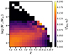 |
Fig. 10. Same as the top panel of Fig. 2 but with the escape fractions obtained using the fitting formula in Eq. (14). |
Figure 11 shows that the fitting formula is able to successfully predict the bimodality in the escape fraction, as seen in Fig. 4. However, the boundary between the two modes is less pronounced. This is likely caused by the smoothing effect of the optimisation process of the fitting function discussed above.
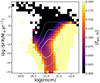 |
Fig. 11. Same as the top panel of Fig. 4 but with the escape fractions obtained using the fitting formula in Eq. (14). |
By comparing Fig. 12 to Fig. 3, we see that the fitting formula is able to reproduce all important trends, namely, the decrease in peak escape fraction with redshift and the approximate locations and values of the peaks. We also reproduce both the minima and maxima in the dependence of fesc on Mgas.
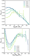 |
Fig. 12. Same as Fig. 3 but with the escape fractions obtained using the fitting formula in Eq. (14). |
Finally, in Fig. 13 we compare the ionising photon escape density obtained using the seminalytic model directly to the results from the semianalytic model. As one can see, the model is highly successful in matching the photon escape at lower stellar masses with higher discrepancies at higher masses. This can be explained given the high numerical abundance of these low-mass galaxies (see Fig. 1) dominated the fitting process. In general, we can say that the fitting model overpredicts the total ionising emissivity density by 10–20%. This discrepancy is not noticeably dependent on redshift and is higher for the ext-mode compared to the loc-mode.
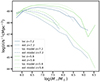 |
Fig. 13. Comparison of the ionising emissivity obtained using the semianalytic model as compared to the fitting formula at two sample redshifts. |
As mentioned earlier, it is important to emphasise that our modelling aims to capture the overall trends of LyC escape with galactic properties. Considering the inherent limitations in resolution and simplifications involved in estimating the LyC flux, it is crucial to scale the absolute value predicted by the fitting formula using a free parameter, which should be determined based on the specific ionising photon budget required for reionisation. We intend to investigate the large-scale implications of these results and to determine scaling parameters in subsequent work.
5. Discussion and conclusions
To gain a better understanding of the correlation of LyC escape with galactic properties, we have applied the physically motivated model for the LyC escape fraction developed in F23 to ≈600 000 galaxies extracted from the TNG50 simulation (Nelson et al. 2019; Pillepich et al. 2019) in the range 5.2 < z < 20. We emphasise that we have employed a very different source model from the one used in our previous study (Kostyuk et al. 2023). In this work, ionising emissivity is sourced by star forming gas rather than by earlier formed star particles. Hence, the ionising emissivity traces the instantaneous star formation rather than its recent history. Therefore, while the underlying simulation in both studies is the same, the difference in the source model strongly limits the correlation between the LyC escape fractions obtained using the two different approaches, as discussed in detail in Appendix C.
Given the large uncertainties in the subgrid modelling of LyC escape, attempting a quantitative comparison of our results to those of previous studies would be impractical. Therefore, we focus our discussion on qualitative results. Numerous previous numerical studies, such as the First Billion Years project (Paardekooper et al. 2015), FIRE-II (Ma et al. 2020), THESAN (Yeh et al. 2023), SPHINX (Rosdahl et al. 2022), and TNG50 (Kostyuk et al. 2023), have consistently demonstrated an increase in the escape fraction with galactic stellar mass, with a maximum reached for galaxies with M⋆ ≈ 107 − 108 M⊙.
The main difference of our work from most previous investigations lies in the prediction of the average escape fraction increasing with decreasing redshift, which we find to be caused by a higher escape fraction from low-mass galaxies at lower redshifts. Furthermore, we find the presence of an additional extended escape mode for high-redshift low-mass galaxies. A potential explanation for the absence of this mode in previous studies, including our own Kostyuk et al. (2023), could be attributed to the predominant reliance on stellar particles as representations of stellar populations. Considering that star formation in the ext-mode takes place across a vast region at a relatively gradual rate, relying on the sampling of relatively massive particles at fixed locations might not provide an accurate depiction of the production of ionising photons in this mode (see Appendix C for a comparison between the two methods). However, given the strong limitation of LyC escape due to dust in the loc-mode, we expect the escape fractions to decline again at even lower redshift. In the future, it will be critical to extend this study to lower redshifts in order to confirm our findings by applying the method to different simulations as well as to investigate what they imply with respect to the reionisation history.
We also note that Katz et al. (2023) identified two distinct modes of LyC escape in the SPHINX simulation, characterised as ‘bursty’ and ‘remnant leakers’, contingent on the galaxies’ SFR. The ‘remnant leakers’ exhibit low SFR values and share a somewhat higher metallicity threshold with the ext-mode in our study. However, the two modes extend to significantly higher stellar masses than our ext-mode. Due to the different methodologies employed in these studies, a more quantitative analysis is necessary before a definitive comparison between the two findings can be established.
Our main results can be summarised as follows:
-
LyC escape is maximum for low-mass galaxies with M⋆ = (106 − 107) M⊙ and then decreases such that galaxies with M⋆ > 109 M⊙ have negligible fesc values.
-
High-redshift galaxies exhibit two main modes of LyC leakage: (a) The ‘extended escape mode’ is characterised by extensive star formation regions, where LyC photons escape from the outer parts of galaxies (Gini score 0.79) with a low gas column density. Galaxies in this mode usually have a higher metal content (10−3.5 < Z < 10−2), which facilitates gas cooling and its collapse onto a thin plane with small-scale heights (H < 8 × 1020 cm), where stars can form over a wide area. Here, dust absorption plays a subdominant role in limiting LyC escape with respect to gas absorption. These galaxies typically have low stellar masses, M⋆ < 107 M⊙, and SFRs, SFR < 10−3 M⊙ yr−1. (b) The ‘localised escape mode’ is characterised by compact ionised channels (with a Gini score of 0.93) in central highly star forming parts of galaxies with large-scale heights (H > 3 × 1021 cm). It is mainly limited by dust opacity, resulting in a negligible LyC escape for galaxies with Z > 10−3 (given our assumption that dust content is linearly correlated with the metallicity). Galaxies leaking LyC through this mode have stellar masses of M⋆ < 108 M⊙ and SFRs in the range 10−5 M⊙ yr−1 < SFR < 1 M⊙ yr−1.
-
The average escape fraction decreases with increasing redshift for galaxies with M⋆ < 107 M⊙. This behaviour is mainly driven by the ext-mode, which represents the main LyC escape channel in low-mass relatively high metallicity galaxies (i.e. the typical properties of high-redshift galaxies). This trend, however, is unlikely to continue to lower redshifts given the eventual quenching of low-mass galaxies in the post-reionisation era.
-
We provide a handy fitting function that predicts the LyC escape fraction of a single galaxy within a factor of approximately two, with a relative deviation of 3.4% in the average escape fraction. Our model is statistically able to capture most features of LyC leakage as a function of galactic properties, such as the bimodality, and the dependence of the escape fraction on redshift, SFR, and stellar mass. This model is well suited to describing the subgrid escape of galaxies for large-scale simulations.
While the model discussed in this paper has been proven effective at characterizing the escape of LyC radiation, in the future we plan to test its validity on different simulations. Additionally, we aim to extend it to account for a more complex structure of the absorbing gas and investigate the relative contribution of the two escape modes to reionisation through cosmic time.
Data availability
Data directly related to this publication and its figures is available on request from the corresponding author. The IllustrisTNG simulations, including TNG50, are publicly available and accessible at https://www.tng-project.org/data/ (see Nelson et al. 2019).
It should be noted that this ratio is based on Milky Way extinction curves and could be sensitive to redshift evolution.
We note that F23 also take into account a reduction in N0 due to radiation pressure pushing out part of the gas. However, as radiation pressure is not explicitly included in the TNG50 simulations, we neglected this effect and adopted the above simplified model.
We note that the while the colour scale saturates the average escape fractions within a given mode keeps increasing following the pattern indicated by the colour gradients.
We do not show Nd here as the map would essentially be fully dark.
Acknowledgments
The authors extend their gratitude to Enrico Garaldi for insightful discussions that have contributed to the development of this work. Furthermore, we would like to express our appreciation to Dylan Nelson and Ruediger Pakmor for their valuable recommendations regarding the post-processing of TNG50 data.
References
- Alavi, A., Colbert, J., Teplitz, H. I., et al. 2020, ApJ, 904, 59 [NASA ADS] [CrossRef] [Google Scholar]
- Asplund, M., Grevesse, N., Sauval, A. J., & Scott, P. 2009, ARA&A, 47, 481 [NASA ADS] [CrossRef] [Google Scholar]
- Boutsia, K., Grazian, A., Giallongo, E., et al. 2011, ApJ, 736, 41 [NASA ADS] [CrossRef] [Google Scholar]
- Chabrier, G. 2003, PASP, 115, 763 [Google Scholar]
- Chisholm, J., Orlitová, I., Schaerer, D., et al. 2017, A&A, 605, A67 [NASA ADS] [CrossRef] [EDP Sciences] [Google Scholar]
- Chisholm, J., Prochaska, J. X., Schaerer, D., Gazagnes, S., & Henry, A. 2020, MNRAS, 498, 2554 [CrossRef] [Google Scholar]
- Chisholm, J., Saldana-Lopez, A., Flury, S., et al. 2022, MNRAS, 517, 5104 [CrossRef] [Google Scholar]
- Ciardi, B., Ferrara, A., Marri, S., & Raimondo, G. 2001, MNRAS, 324, 381 [NASA ADS] [CrossRef] [Google Scholar]
- Davis, M., Efstathiou, G., Frenk, C. S., & White, S. D. 1985, ApJ, 292, 371 [NASA ADS] [CrossRef] [Google Scholar]
- Dayal, P., & Ferrara, A. 2018, Physics Reports, 780, 1 [CrossRef] [Google Scholar]
- Dayal, P., Ferrara, A., Sommovigo, L., et al. 2022, MNRAS, 512, 989 [NASA ADS] [CrossRef] [Google Scholar]
- Dijkstra, M., Wyithe, S., Haiman, Z., Mesinger, A., & Pentericci, L. 2014, MNRAS, 440, 3309 [CrossRef] [Google Scholar]
- Faucher-Giguère, C.-A., Lidz, A., Zaldarriaga, M., & Hernquist, L. 2009, ApJ, 703, 1416 [Google Scholar]
- Ferrara, A., Vallini, L., Pallottini, A., et al. 2019, MNRAS, 489, 1 [Google Scholar]
- Grazian, A., Giallongo, E., Gerbasi, R., et al. 2016, A&A, 585, A48 [NASA ADS] [CrossRef] [EDP Sciences] [Google Scholar]
- Graziani, L., Maselli, A., & Ciardi, B. 2013, MNRAS, 431, 722 [CrossRef] [Google Scholar]
- Heckman, T. M., Sembach, K. R., Meurer, G. R., et al. 2001, ApJ, 558, 56 [Google Scholar]
- Inoue, A. K., Iwata, I., & Deharveng, J.-M. 2006, MNRAS, 371, L1 [NASA ADS] [CrossRef] [Google Scholar]
- Jones, T. A., Ellis, R. S., Schenker, M. A., & Stark, D. P. 2013, ApJ, 779, 52 [Google Scholar]
- Katz, H., Saxena, A., Rosdahl, J., et al. 2023, MNRAS, 518, 270 [Google Scholar]
- Kimm, T., & Cen, R. 2014, ApJ, 788, 121 [NASA ADS] [CrossRef] [Google Scholar]
- Kostyuk, I., Nelson, D., Ciardi, B., Glatzle, M., & Pillepich, A. 2023, MNRAS, 521, 3077 [CrossRef] [Google Scholar]
- Leitet, E., Bergvall, N., Piskunov, N., & Andersson, B. G. 2011, A&A, 532, A107 [NASA ADS] [CrossRef] [EDP Sciences] [Google Scholar]
- Leitherer, C., Schaerer, D., Goldader, J. D., et al. 1999, ApJS, 3 [Google Scholar]
- Lewis, J. S., Ocvirk, P., Aubert, D., et al. 2020, MNRAS, 496, 4342 [NASA ADS] [CrossRef] [Google Scholar]
- Ma, X., Hopkins, P. F., Kasen, D., et al. 2016, MNRAS, 459, 3614 [Google Scholar]
- Ma, X., Quataert, E., Wetzel, A., et al. 2020, MNRAS, 498, 2001 [Google Scholar]
- Marinacci, F., Vogelsberger, M., Pakmor, R., et al. 2018, MNRAS, 480, 5113 [NASA ADS] [Google Scholar]
- Maselli, A., Ferrara, A., & Ciardi, B. 2003, MNRAS, 345, 379 [CrossRef] [Google Scholar]
- Maselli, A., Ciardi, B., & Kanekar, A. 2009, MNRAS, 393, 171 [CrossRef] [Google Scholar]
- Matthee, J., Sobral, D., Best, P., et al. 2016, MNRAS, 465, 3637 [Google Scholar]
- Mostardi, R. E., Shapley, A. E., Nestor, D. B., et al. 2013, ApJ, 779, 65 [NASA ADS] [CrossRef] [Google Scholar]
- Naiman, J. P., Pillepich, A., Springel, V., et al. 2018, MNRAS, 477, 1206 [Google Scholar]
- Nakajima, K., & Ouchi, M. 2014, MNRAS, 442, 900 [Google Scholar]
- Nelson, D., Pillepich, A., Springel, V., et al. 2018, MNRAS, 475, 624 [Google Scholar]
- Nelson, D., Pillepich, A., Springel, V., et al. 2019, Computational Astrophysics and Cosmology, 6, 2 [CrossRef] [Google Scholar]
- Nestor, D. B., Shapley, A. E., Steidel, C. C., & Siana, B. 2011, ApJ, 736, 18 [NASA ADS] [CrossRef] [Google Scholar]
- Ocvirk, P., Gillet, N., Shapiro, P. R., et al. 2016, MNRAS, 463, 1462 [Google Scholar]
- Ocvirk, P., Lewis, J. S., Gillet, N., et al. 2021, MNRAS, 507, 6108 [NASA ADS] [CrossRef] [Google Scholar]
- Paardekooper, J. P., Khochfar, S., & Vecchia, C. D. 2015, MNRAS, 451, 2544 [CrossRef] [Google Scholar]
- Pahl, A. J., Shapley, A., Steidel, C. C., Chen, Y., & Reddy, N. A. 2021, MNRAS, 505, 2447 [NASA ADS] [CrossRef] [Google Scholar]
- Pillepich, A., Springel, V., Nelson, D., et al. 2018a, MNRAS, 473, 4077 [Google Scholar]
- Pillepich, A., Nelson, D., Hernquist, L., et al. 2018b, MNRAS, 475, 648 [Google Scholar]
- Pillepich, A., Nelson, D., Springel, V., et al. 2019, MNRAS, 490, 3196 [Google Scholar]
- Planck Collaboration I. 2016, A&A, 594, A1 [NASA ADS] [CrossRef] [EDP Sciences] [Google Scholar]
- Rosdahl, J., Katz, H., Blaizot, J., et al. 2018, MNRAS, 479, 994 [NASA ADS] [Google Scholar]
- Rosdahl, J., Blaizot, J., Katz, H., et al. 2022, MNRAS, submitted [arxiv:2207.03232] [Google Scholar]
- Springel, V. 2010, MNRAS, 401, 791 [Google Scholar]
- Springel, V., & Hernquist, L. 2003, MNRAS, 339, 289 [Google Scholar]
- Springel, V., White, S. D., Tormen, G., & Kauffmann, G. 2001, MNRAS, 328, 726 [NASA ADS] [CrossRef] [Google Scholar]
- Springel, V., White, S. D. M., Jenkins, A., et al. 2005, Nature, 435, 629 [Google Scholar]
- Springel, V., Pakmor, R., Pillepich, A., et al. 2018, MNRAS, 475, 676 [Google Scholar]
- Tang, M., Stark, D., Chevallard, J., et al. 2021, MNRAS, 705, 503 [Google Scholar]
- Vanzella, E., Giavalisco, M., Inoue, A. K., et al. 2010, ApJ, 725, 1011 [NASA ADS] [CrossRef] [Google Scholar]
- Verhamme, A., Orlitová, I., Schaerer, D., & Hayes, M. 2015, A&A, 578, A7 [NASA ADS] [CrossRef] [EDP Sciences] [Google Scholar]
- Weinberger, R., Springel, V., Hernquist, L., et al. 2017, MNRAS, 465, 3291 [Google Scholar]
- Weingartner, J. C., & Draine, B. T. 2001, ApJ, 548, 296 [Google Scholar]
- Xu, H., Wise, J. H., Norman, M. L., Ahn, K., & O’Shea, B. W. 2016, ApJ, 833, 84 [NASA ADS] [CrossRef] [Google Scholar]
- Yeh, J. Y. C., Smith, A., Kannan, R., et al. 2023, MNRAS, 520, 2757 [NASA ADS] [CrossRef] [Google Scholar]
Appendix A: Convergence with grid size
In order to accurately capture the escape of LyC radiation, we need to ensure that the galaxies are sufficiently resolved. In our approach, we distribute the gas particles of the TNG50 galaxy, as well as their physical properties, on a regular Cartesian grid before projecting all galactic properties as surface densities onto the galactic plane. To ensure the escape fraction we obtain is sufficiently resolved, we applied this method to a sample of galaxies varying the grid sizes in the range of 23 to 5023 in steps of 20. We used a sample of 80 galaxies. To ensure that the sample represents the range of galaxies in the TNG50 simulation, the halos were sampled from logarithmically spaced stellar mass bins, ranging from the least to the most massive galaxies in the simulation.
The result of the convergence study can be seen in Fig. A.1. We observe that fesc rapidly converges with the grid size. In other words, there is no significant change in fesc for grid sizes > 603. The increase in fesc for small grid sizes is explained by the smoothing out of regions containing dense gas, thus decreasing its optical depth. Finally, at grid sizes > 1503 in some galaxies the escape fraction increases, while for a few others it becomes undefined. This is likely caused by numerical problems as in some grid cells the smoothing kernel decreases to small, numerically unstable values. Based on these results we have chosen 1003 grid cells to be a reliable number to ensure that the LyC escape fraction is fully resolved within the resolution limits of the TNG50 simulation itself.
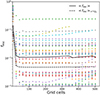 |
Fig. A.1. Escape fraction of a sample of galaxies as a function of the number of grid cells per dimension. We additionally depict the average escape fraction (black continuous line) and the average escape fraction weighted by the emissivity (black dashed line). |
Appendix B: Extent of the star forming regions
As discussed previously, our model assumes that star formation, and hence LyC production, takes place in a thin slab. This assumption is based on the fact that most star formation is confined to a region significantly narrower than the one occupied by the gas, which inhibits radiation escape. Consequently, a substantial portion of LyC photons is required to traverse the majority of the intervening gas.
While this intuitively holds for large, disc-shaped galaxies, its validity may be questioned when applied to smaller galaxies that exhibit a more spherical morphology. In order to verify this assumption, we examine the ratio between the scale height of the star forming region (HSFR) and that of the gas (Hgas), as illustrated in Fig. B.1.
Our analysis reveals an average ratio of approximately 0.6, implying that in most galaxies, on average, the star forming region is considerably closer to the centre than the majority of the gas. Although this value suggests that our model might overlook some potential LyC escape originating from star forming regions positioned above the galactic plane, given the qualitative and statistical nature of our study, the model provides a reasonable estimate of the likelihood of LyC radiation escaping.
Notably, we see a lack of substantial evolution in the ratio with increasing stellar mass. Indeed, galaxies with higher stellar masses tend collapse into a more disc-like structure, that is a lower scale height of the star forming region. However, the gas enveloping the galaxy is also more collapsed, resulting in a ratio that is not too dissimilar from that of smaller galaxies.
Although a larger number of galaxies exhibit higher values of HSFR/Hgas for smaller M⋆, this pattern arises solely from the larger sample size. This is evident as the width of the 1-sigma scatter of HSFR/Hgas values remains relatively constant across the entire stellar mass range.
Summarising, despite the fact that smaller galaxies have a much more diffuse structure, the thin slate assumption should still hold for the galaxy population as a whole (although this is not the case for single galaxies) given that the LyC producing region is significantly thinner than the distribution of the gas inhibiting its escape.
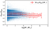 |
Fig. B.1. Ratio between the scale height of the star forming region and that of the gas as a function of galactic stellar mass. The red line represents the average value of this ratio, and the errorbars its one sigma scatter. The linear pattern in which the points appear is a consequence of measuring the scale height in discrete grid cell numbers. |
Appendix C: Comparison with numerical post-processing
In Kostyuk et al. (2023) we investigated the escape fraction of ∼104 galaxies from TNG50 using the Monte-Carlo RT code CRASH (Ciardi et al. 2001; Maselli et al. 2009, 2003; Graziani et al. 2013). While there is an overlap in the galaxies that we have examined the methodology significantly differs.
In Fig. C.1 we depict projections of one example galaxy that was examined in both Kostyuk et al. (2023) and this work. In the former study the escape fraction was determined to be fesc, RT = 63.5% while in this study it yielded fesc = 12.7%. We note that the orientation of the galaxy differs as the gas in the RT case was gridded with respect to its TNG50 coordinates as photon emission takes place isotropically in the simulation and is therefore orientation invariant, while, as described in Sect. 2, in the semianalytic case the galaxy was first rotated into the galactic plane.
Given that we used different properties to calculate the escape fraction the characteristics that we depict in the plots are naturally also different. The relevant quantities to determine the escape fraction in the RT study were the gas density, the ionisation fraction of that gas and finally the distribution of the ionising sources. We see that while most of the gas is ionised, the escape fraction is reduced by neutral gas patches in the lower-half of central region as well as in the lower centre of the galaxy. However, even in the central region most of the gas is ionised allowing for ionising radiation to escape from the area of its highest production.
In the semianalytic study we see that the ionising flux derived from the SFR does approximately trace the distribution of ionising sources on the left. However, as one can see by the optical depth and escape fraction distribution, ionising photons are fully absorbed in the central region of the galaxy, thus resulting in a much lower escape fraction as in the RT approach. It is likely that the discrepancy can be attributed to the smoothing out of the production area of ionising photons and the resulting increase of the gas to photon ratio.
Next we inspect the escape fractions of all galaxies processed with our two methods. In Fig. C.2 we plot the escape fractions obtained here, fesc, as a function of those evaluated in Kostyuk et al. (2023), fesc, RT. Surprisingly, only for fesc, RT > 0.6 a slight correlation between the values obtained in the two studies can be seen.
We believe that the reason for this behaviour is the different methodology used for obtaining the ionising emissivity of a galaxy. Indeed, in the numerical approach this was determined for individual stellar particles representing a whole stellar population, since CRASH evaluates the propagation of photons emitted by the discrete sources. Moreover, the information encapsulated in the stellar particles, such as age, metallicity, and mass, allowed us to compute the full ionising spectrum, enabling an investigation of LyC escape in individual frequency bins. On the other hand, the SFR is a better tracer of the location of new stars, which are expected to emit most ionising radiation. Additionally, a stellar particle-based approach in our semi-analytic model would lack numerical stability under grid refinement. Indeed, because of the fixed emissivity of star particles, a smaller grid-size would always result in a larger flux in cells hosting such particles.
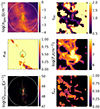 |
Fig. C.1. Comparison between a galaxy processed with CRASH-RT (left) and one processed with the semianalytic model (right). On the left we depict from top to bottom the average gas density (ngas), the average ionisation fraction (xHII) and the distribution and ionising emissivity of sources (Qsources). On the right we depict the hydrogen optical depth (τHI), ionising emissivity Fion and the location based escape fraction (fesc). |
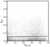 |
Fig. C.2. Escape fractions obtained using the analytic method discussed here, fesc, as a function of those obtained by post-processing the galaxies with the RT code CRASH, fesc, RT. The line represents a linear fit to the data. |
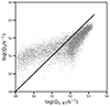 |
Fig. C.3. Ionising emissivity obtained from the SFR of galaxies, Q0, as a function of that calculated using the spectra of stellar particles, Q0, RT. The line represents a 1:1 correspondence. |
The difference introduced by the two approaches can be appreciated in fig C.3, where the emissivities for a given galaxy obtained with the stellar particle, Q0, RT, and with the SFR, Q0, are plotted. It is evident that the scatter is very large, in particular for Q0, RT < 1052s−1, where more than one order of magnitude difference is observed. The reason for this is that smaller galaxies contain very few stellar particles such that random fluctuations in the spawning of one young stellar particle induce a large difference in the ionising emissivity. The effect becomes less visible in larger galaxies, explaining the stronger correlation seen for Q0, RT > 1052s−1.
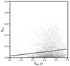 |
Fig. C.4. Same as Fig. C.2 but only for galaxies with Q0, RT > 1052 s−1. The line represents a linear fit to the data. |
This is reflected in fig C.4, where we consider only the escape fraction of galaxies with Q0, RT > 1052s−1, for which the correlation between the two escape fractions is much stronger. However, the scatter is still significant due to the geometry of the problem. Indeed, here the full star forming regions are considered as source of radiation, meaning that LyC emission is less concentrated and thus less sensitive to the fluctuation in the densities of the surrounding gas. This is not the case for stellar particles, when the escape fraction can change significantly because of random fluctuations in the relative position of a stellar particle and the surrounding gas. Finally, differently from the analytic approach, the numerical study models the radiation transfer of ionising radiation.
Finally, in Fig. C.5 we show the evolution of fesc with stellar mass for the two approaches. Besides the main quantitative discrepancy in the values of the escape fraction we see two main differences in these results. Namely, the peak escape fraction is located at significantly higher stellar mass values in case of the RT approach. Most importantly, however, is the different evolution with redshift. As discussed earlier this discrepancy is likely to be caused by the ext-mode that emerges in the semianalytic model but is not present in the RT model due to the Poissonian sampling of the emitters of ionising radiation.
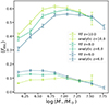 |
Fig. C.5. Comparison of fesc dependence on stellar mass for the RT and semianalytic approaches. |
All Figures
|
Fig. 1. Number of galaxies processed as a function of redshift (top) and as a function of stellar mass (bottom). |
| In the text | |
|
Fig. 2. Average LyC escape fraction of all galaxies in a given bin (colour scale) as a function of redshift and galactic stellar mass (top) as well as gas mass (bottom). The white contours denote the 1 (solid), 2 (dashed) and 3 (dotted) sigma distribution of galaxy counts. |
| In the text | |
|
Fig. 3. Average LyC escape fraction as a function of stellar mass (top) and gas mass (bottom) for a sample of redshifts. The error bars denote the statistical error of the mean. |
| In the text | |
|
Fig. 4. Average escape fraction as a function of scale height and SFR (top) as well as a function of scale height and galactic stellar mass (bottom). The contours represent the distribution of galaxies as described in Fig. 2. The numbers label the areas that we identified as the localised escape mode (loc-mode, number 1), the extended escape mode (ext-mode, number 2) and the LyC dark mode (number 3). |
| In the text | |
|
Fig. 5. Comparison of the escape density of the ionising photons from the loc-mode (solid) and ext-mode (dashed) as a function of stellar mass (left) and well as the cumulative escape (right). |
| In the text | |
|
Fig. 6. Projected maps of the escape fraction; ionising flux, Fi; and the gas optical depth, τHI, distribution from individual grid cells (box size 4 stellar half mass radii) for three example galaxies from the loc-mode (top panels), ext-mode (centre), and LyC dark mode (bottom). |
| In the text | |
|
Fig. 7. Galaxies with scale heights H > 1021.3 cm selected for their high and low SFR, that is log(SFR/M⊙ yr−1)=0.14, 0.20, and 0.40 (top) and log(SFR/M⊙ yr−1)= − 4.34, −4.05, and −4.08 (bottom figure). From top to bottom, the panels in each figure refer to the cell escape fraction, fesc, cell; optical depth of dust, τd; and of gas, τHI. |
| In the text | |
|
Fig. 8. Average escape fraction as a function of metallicity and galactic gas mass (top panels), metallicity and galactic stellar mass (centre), and SFR and stellar mass (bottom). The left and right columns refer to galaxies with log(H/cm)< 20.8 and log(H/cm)> 21.3, which include the ext- and loc-modes, respectively. The contours denote the 1 (solid), 2 (dashed) and 3 (dotted) sigma distribution of galaxy counts. |
| In the text | |
|
Fig. 9. Redshift evolution of the average escape fraction as a function of SFR (upper panel) and scale height (lower). The contours denote the 1 (solid), 2 (dashed) and 3 (dotted) sigma distribution of galaxy counts. |
| In the text | |
|
Fig. 10. Same as the top panel of Fig. 2 but with the escape fractions obtained using the fitting formula in Eq. (14). |
| In the text | |
|
Fig. 11. Same as the top panel of Fig. 4 but with the escape fractions obtained using the fitting formula in Eq. (14). |
| In the text | |
|
Fig. 12. Same as Fig. 3 but with the escape fractions obtained using the fitting formula in Eq. (14). |
| In the text | |
|
Fig. 13. Comparison of the ionising emissivity obtained using the semianalytic model as compared to the fitting formula at two sample redshifts. |
| In the text | |
|
Fig. A.1. Escape fraction of a sample of galaxies as a function of the number of grid cells per dimension. We additionally depict the average escape fraction (black continuous line) and the average escape fraction weighted by the emissivity (black dashed line). |
| In the text | |
|
Fig. B.1. Ratio between the scale height of the star forming region and that of the gas as a function of galactic stellar mass. The red line represents the average value of this ratio, and the errorbars its one sigma scatter. The linear pattern in which the points appear is a consequence of measuring the scale height in discrete grid cell numbers. |
| In the text | |
|
Fig. C.1. Comparison between a galaxy processed with CRASH-RT (left) and one processed with the semianalytic model (right). On the left we depict from top to bottom the average gas density (ngas), the average ionisation fraction (xHII) and the distribution and ionising emissivity of sources (Qsources). On the right we depict the hydrogen optical depth (τHI), ionising emissivity Fion and the location based escape fraction (fesc). |
| In the text | |
|
Fig. C.2. Escape fractions obtained using the analytic method discussed here, fesc, as a function of those obtained by post-processing the galaxies with the RT code CRASH, fesc, RT. The line represents a linear fit to the data. |
| In the text | |
|
Fig. C.3. Ionising emissivity obtained from the SFR of galaxies, Q0, as a function of that calculated using the spectra of stellar particles, Q0, RT. The line represents a 1:1 correspondence. |
| In the text | |
|
Fig. C.4. Same as Fig. C.2 but only for galaxies with Q0, RT > 1052 s−1. The line represents a linear fit to the data. |
| In the text | |
|
Fig. C.5. Comparison of fesc dependence on stellar mass for the RT and semianalytic approaches. |
| In the text | |
Current usage metrics show cumulative count of Article Views (full-text article views including HTML views, PDF and ePub downloads, according to the available data) and Abstracts Views on Vision4Press platform.
Data correspond to usage on the plateform after 2015. The current usage metrics is available 48-96 hours after online publication and is updated daily on week days.
Initial download of the metrics may take a while.