| Issue |
A&A
Volume 691, November 2024
|
|
|---|---|---|
| Article Number | A314 | |
| Number of page(s) | 13 | |
| Section | Astrophysical processes | |
| DOI | https://doi.org/10.1051/0004-6361/202452069 | |
| Published online | 21 November 2024 | |
An acceleration-radiation model for nonthermal flares from Sgr A*
1
Department of Physics, National and Kapodistrian University of Athens, University Campus Zografos, GR 15784 Athens, Greece
2
Institute of Accelerating Systems & Applications, University Campus Zografos, GR 15784 Athens, Greece
3
Max-Planck-Institut für Extraterrestrische Physik, Giessenbachstrasse, 85748 Garching, Germany
4
INAF – Osservatorio Astronomico di Brera, Via E. Bianchi 46, 23807 Merate, Italy
5
DiSAT, Università degli Studi dell’Insubria, Via Valleggio 11, I-22100 Como, Italy
⋆ Corresponding author; This email address is being protected from spambots. You need JavaScript enabled to view it.
Received:
30
August
2024
Accepted:
3
October
2024
Abstract
Context. Sgr A⋆ is the electromagnetic counterpart of the accreting supermassive black hole in the Galactic center. Its emission is variable in the near-infrared (NIR) and X-ray wavelengths on short timescales (several minutes to a few hours). The NIR light curve displays red-noise variability, while the X-ray light curve exhibits bright flares that rise by many orders of magnitude upon the stable X-ray quiescent emission. Every X-ray flare is associated with a bright NIR flux change, but the opposite is not always true. The physical origin of NIR and X-ray flares is still under debate.
Aims. We introduce a model for the production of NIR and X-ray flares from an active region in Sgr A⋆, where particle acceleration takes place intermittently. A fraction of electrons from their thermal pool is accelerated to higher energies while they radiate via synchrotron and synchrotron self-Compton (SSC) processes. In contrast to other radiation models for Sgr A⋆ flares, the particle acceleration is not assumed to be instantaneous.
Methods. We studied the evolution of the particle distribution and the emitted electromagnetic radiation from the flaring region by numerically solving the kinetic equations for electrons and photons. Our calculations took the finite duration of particle acceleration, radiative energy losses, and physical escape from the flaring region into account. To gain better insight into the relation of the model parameters, we complemented our numerical study with analytical calculations.
Results. Flares are produced when the acceleration episode has a finite duration. The rising part in the light curve of a flare is related to the particle acceleration timescale, while the decay is controlled by the cooling or escape timescale of particles. The emitted synchrotron spectra are power laws whose photon index is determined by the ratio of the acceleration and escape timescales, followed by an exponential cutoff. This occurs at the characteristic synchrotron photon energy emitted by particles with the maximum Lorentz factor (where energy loss and gain rates become equal). The NIR flux increases before the onset of the X-ray flare, and the time lag is linked to the particle acceleration timescale. Bright X-ray flares, such as the one observed in 2014, have γ-ray counterparts that might be detected by the Cherenkov Telescope Array Observatory.
Conclusions. Our generic model for NIR and X-ray flares favors an interpretation of diffusive nonresonant particle acceleration in magnetized turbulence. If direct acceleration by the reconnection electric field in macroscopic current sheets causes the energization of particles during flares in Sgr A⋆, then models considering the injection of preaccelerated particles into a blob where particles cool and/or escape would be appropriate to describe the flare.
Key words: radiation mechanisms: non-thermal / radiative transfer / Galaxy: center
© The Authors 2024
 Open Access article, published by EDP Sciences, under the terms of the Creative Commons Attribution License (https://creativecommons.org/licenses/by/4.0), which permits unrestricted use, distribution, and reproduction in any medium, provided the original work is properly cited.
This article is published in open access under the Subscribe to Open model. This email address is being protected from spambots. You need JavaScript enabled to view it. to support open access publication.
1. Introduction
Sgr A⋆, the radiative counterpart of the supermassive black hole at the Galactic center, is considered to be one of the best targets for studying accretion physics at low luminosity (Genzel et al. 2010). The combination of its low bolometric luminosity (about L ∼ 1036 erg s−1) and close distance to us makes it one of the few low-luminosity active galactic nuclei (AGN) on which we can study accretion physics at exceptionally low Eddington ratios (∼10−8) in great detail.
The electromagnetic spectrum of Sgr A⋆ peaks in the submillimeter band, where it forms the so-called submm bump (Yuan et al. 2003), which has recently been imaged by the Event Horizon Telescope Collaboration (EHT Collaboration 2022). It is thought to be due to optically thick synchrotron radiation produced by relativistic quasi-thermal electrons with a temperature Te∼ few 1010 K (or typical Lorentz factor γ ∼ 10) and a density ne ∼ 106 cm−3, embedded in a magnetic field with a strength of ∼10 − 50 G (Loeb & Waxman 2007; Genzel et al. 2010).
In the near-infrared (NIR) band, Sgr A⋆ displays a red-noise light curve at frequencies higher than a fraction of a day, showing continuous variations with multiple peaks and no obvious quiescent state (Do et al. 2009; Witzel et al. 2012, 2018). With the Gravity interferometer, it has been possible to determine the evolution of the astrometry and polarization of the source during bright NIR events (GRAVITY Collaboration 2018, 2020). During flares, the NIR source appears to be compact (R < 2 − 3 RS)1 and to move at ∼30% of the speed of light. It traces loops on the sky with a radius of about six to ten gravitational radii. At the same time, the NIR polarization angle is observed to rotate. The swings in the polarization angle are consistent with a model in which the synchrotron-emitting flaring region is embedded in a poloidal magnetic field configuration and rotates approximately consistently with the observed astrometric loops (GRAVITY Collaboration 2018, 2020).
In the X-ray band, Sgr A⋆ displays a quiescent luminosity of L2 − 10 keV ∼ 2 × 1033 erg s−1 (Baganoff et al. 2003; Xu et al. 2006). This quiescent emission is thought to be produced via bremsstrahlung radiation from a hot plasma with a density of ne ∼ 10−3 cm−3 and a temperature T ∼ 7 × 10⁷ K in a region with a size of ∼105RS. It is likely associated with the accretion of winds from nearby massive stars (Melia 1992; Quataert 2002; Cuadra et al. 2006, 2008). Upon this stable quiescent emission, the X-ray light curve exhibits bright flares that typically last for a small fraction of the time (from several minutes to a few hours). This suggests that flares are individual events that randomly punctuate an otherwise quiescent source (Neilsen et al. 2013; Ponti et al. 2015). Moreover, it is observed that every X-ray flare has an NIR counterpart (i.e., it is associated with a bright NIR flux excursion), but most NIR flares have no X-ray counterpart.
X-ray flares have a power-law luminosity distribution (dN/dL) with a slope of ∼ − 1.9, and the moderate flares (L2 − 8 keV ≈ 1034 erg s−1) occur about once per day (Degenaar et al. 2013; Neilsen et al. 2013, 2015; Ponti et al. 2015). It is still debated whether the flaring rate is stationary or changes over time, or if the flares preferentially occur in clusters (Ponti et al. 2015; Yuan & Wang 2016; Mossoux et al. 2016; Mossoux & Grosso 2017; Bouffard et al. 2019; Andrés et al. 2022). The duration and fluence of the X-ray flares have power-law distributions with observed fluences in the range ∼10−9 − 10−7 erg cm−2 and durations from several minutes to a few hours (Neilsen et al. 2013; Ponti et al. 2015; Yuan & Wang 2016).
According to the canonical szenario for the production of flares at NIR and X-ray energies, a small region in the accretion flow appears to energize electrons well beyond their typical thermal energy. While synchrotron radiation of nonthermal electrons causes the observed NIR emission (Genzel et al. 2010), the origin of the X-ray emission is still debated. Several radiative mechanisms have been proposed to explain the X-ray flaring emission, including synchrotron, synchrotron self-Compton (SSC), and inverse Compton (IC) on submm seed photons within tens of Schwarzschild radii from Sgr A⋆ (Markoff et al. 2001; Yuan et al. 2003; Eckart et al. 2004, 2008; Yusef-Zadeh et al. 2006, 2008; Hornstein et al. 2007; Marrone et al. 2008; Dodds-Eden et al. 2010; Trap et al. 2011; Dibi et al. 2014; Gutiérrez et al. 2020; Witzel et al. 2021). Regardless of the X-ray production mechanism, most models describe the emission arising from a source into which preaccelerated electrons are injected, which is subsequently left to cool through radiative and/or adiabatic losses. It is therefore implicitly assumed that the acceleration of particles occurs instantaneously compared to all other relevant timescales.
We present an acceleration-radiation model for the production of NIR and X-ray flares from an active region of the accretion flow. Our goal is to present an alternative interpretation for the NIR and X-ray flares of Sgr A⋆ that is inspired by a model that was originally proposed for AGN flares (Kirk et al. 1998); see also Mastichiadis & Moraitis (2008). We study the energization of electrons from their thermal pool to higher energies in a time-dependent way and account for their synchrotron and SSC emission. This is in contrast to other radiation models, in which the acceleration phase of the particles is usually not taken into account (because it is assumed to be instantaneous, e.g.). Our study is motivated by multiwavelength observations of Sgr A⋆ during bright flares, which show evidence for a later onset of the X-ray flare than in its NIR counterpart (Ponti et al. 2017; GRAVITY Collaboration 2021). An exciting possibility would be that we observing in real time particle energization in the vicinity of Sgr A⋆.
This paper is structured as follows. In Sect. 2 we introduce the flare model and provide analytical expressions for the electron distribution and magnetic field strength in the flaring region. We also describe the numerical code we used to calculate the radiative transfer. In Sect. 3 we present numerical results for the time evolution of the spectral energy distribution (SED) and the NIR and X-ray light curves produced in our flare model for constant and time-variable particle injection into the acceleration process. In Sect. 4 we apply our model to the 2014 NIR and X-ray flares of Sgr A⋆. We discuss our results in Sect. 5 and present our main conclusions in Sect. 6.
2. Flare model
2.1. Model description
We assumed that the nonthermal NIR and X-ray flares of Sgr A⋆ are produced from an active region in the vicinity of the black hole (inner accretion flow or boundary between the funnel and the accretion disk), where particle acceleration takes place intermittently. The rising part of the flares is then attributed to the time when the acceleration is active and the decay when the accelerated particles are left to cool radiatively.
The active region (or blob) is described as a spherical and homogeneous region of radius R that contains relativistic electrons and a mean magnetic field of strength B. Particles with an initial Lorentz factor γ0 ≳ 1 that enter the active region at a rate Q0 accelerate to higher Lorentz factors on a timescale tacc, while they can escape the acceleration region on a timescale tesc. Particles also lose energy via synchrotron radiation. We limited our analytical calculations to cases in which inverse-Compton losses are subdominant, and thus, they cannot influence the electron distribution function.
The temporal evolution of the particle distribution, Ne(γ, t), is described by a partial differential equation (PDE) (Kirk et al. 1998),
 (1)
(1)
where bs = σTB2/(6πmec), and δ(x) is the Dirac delta function. If tacc, tesc are independent of the particle Lorentz factor2, and Q0 is a constant, then Eq. (1) has a simple analytical solution, (Kirk et al. 1998)
 (2)
(2)
where N0 = Q0taccγ0tacc/tesc(1−γ0/γsat)−tacc/ttesc, s = 1 + tacc/tesc, and
 (3)
(3)
is the saturation Lorentz factor (where the energy-loss rate balances the energy-gain rate due to acceleration). In Eq. (2), γmax is the upper cutoff of the electron distribution, which evolves with time as
 (4)
(4)
We note that γmax approaches the saturation Lorentz factor for t ≫ tacc only asymptotically.
Because γmax increases monotonically with time during the acceleration phase, the synchrotron flux increases from longer to shorter wavelengths as the synchrotron cutoff frequency sweeps across the electromagnetic spectrum. If the acceleration acts upon particles indefinitely, the electron and photon distributions become stationary. In other words, a flare can be produced when the acceleration lasts for a finite time interval; this will become clearer in Sect. 3.
The optically thin synchrotron spectrum produced by electrons with γ ≪ γsat can be written as (Rybicki & Lightman 1986)
 (5)
(5)
where  is the total number of electrons (at saturation)3, C is a numerical constant that depends on s as
 (6)
(6)
and the synchrotron spectrum photon index is
 (7)
(7)
If the latter is measured in the NIR band, for instance, then we can infer the ratio of the acceleration and escape timescales, tacc/tesc = 2(sph, NIR − 1).
In our model, the X-ray synchrotron radiation is produced by electrons with γ ≈ γsat. We can then estimate the required magnetic field for electrons with γsat to radiate synchrotron photons at a known photon energy ϵX as
 (8)
(8)
where Bcr ≃ 4.4 × 10¹³ G. The numerical value in the above equation was obtained for parameters that were also used in our numerical study in Sect. 3, namely tacc/tesc = 1.5, tesc = R/c ≃ 400 s, for R = 9.5RS, and RS = 2GM/c2 is the Schwarzschild radius of a 4.3 × 10⁶ M⊙ black hole (GRAVITY Collaboration 2019).
Given the inferred magnetic field strength, we can estimate the cooling timescale of electrons radiating at NIR frequencies, νNIR ∼ 1014 Hz,
 (9)
(9)
If the particles remain confined in the flaring region after the end of the acceleration phase, the long cooling timescale of NIR-emitting electrons would suggest an almost constant NIR flux over day-long timescales. Meanwhile, the short cooling timescale of electrons emitting at 10 keV (∼0.3 h for B ∼ 1 G) would result in a fast decrease in the X-ray flux. In this case, the NIR and X-ray flares would have different decaying profiles. A decrease in the NIR flux on much shorter timescales than tcool(νNIR) would require particle escape from the flaring region. In this case, the decaying profiles of NIR and X-ray flares would be similar, dictated by the photon-crossing timescale.
To model the decaying part of the flare, we assumed that the acceleration had ceased while particles were left to cool due to radiative losses and also escaped from the blob (similar to the radiation zone of the two-zone model of Kirk et al. 1998). The kinetic equation for the decay phase of the flare is then written as
 (10)
(10)
where we allowed for a different escape timescale of particles from the active region after the end of the acceleration episode by introducing the parameter  . We assumed that the acceleration ceased when γmax(t = tpk) = ξγsat with ξ ≲ 1. Solving Eq. (4) for tpk, we find an estimate for the peak time of the flare (see also Sect. 3),
 (11)
(11)
For t > tpk, Eq. (10) can be solved using Ne(γ, t = tpk) as an initial condition, where Ne is given by Eq. (2), resulting in
 (12)
(12)
In the postacceleration phase, adiabatic expansion of the blob and magnetic field decay could become relevant. Their impact on the flare decay profile has been investigated in detail in earlier studies (Dodds-Eden et al. 2010).
2.2. Numerical approach
We used the leptonic module of the numerical code atheνa (Dimitrakoudis et al. 2012), which computes the temporal evolution of the lepton (electrons and positrons, Ne(γ, t)) and photon distributions Nph(ϵ, t) (differential in energy)4 by solving a set of coupled PDEs (see below) using a backward-differentiation algorithm with a variable time step,
 (13)
(13)
 (14)
(14)
where tesc = R/c. The operators ℒij and 𝒬ij denote the loss (sink terms) and production (source terms) rates of particle species i due to the process j. The physical processes that are included in the code and couple photons with leptons are electron synchrotron emission, synchrotron self-absorption, electron inverse-Compton scattering, and γγ pair production. Finally, an acceleration term was added to the kinetic equation of electrons, according to Eq. (1). This term is nonzero for a finite duration T, which is a free parameter. To model the decaying part of the flare, we set the acceleration term to zero for t ≥ T.
The code takes as an input the electron compactness, ℓe, which is the dimensionless measure of the injection power of electrons with γ0, and is defined as5
 (15)
(15)
where Q0 is the injection rate of electrons at γ0. Given that Q0 ∝ Ne, tot/tacc, the injection rate at γ0 can be inferred from the observed flare luminosity (see Eq. (5)) for a given tacc. The numerical approach also offers the flexibility of studying time-variable injection rates, that is, Q0 can depend explicitly on time (see Sect. 3.2).
After solving Eqs. (13) and (14), we can compute the escaping photon spectrum from the spherical blob of radius R at time t as L(ϵ, t) = 3mec2ϵNph(ϵ, t)/tesc, where L(ϵ, t) is the escaping photon luminosity at time t per photon energy ϵ. Noting that ϵ = hν/(mec2), we may write Lν(t) = hL(ϵ, t)/(mec2), where h is the Planck constant. The differential flux Fν measured by an observer at a distance D is then Fν(t) = Lν(t)/(4πD2). The light curves are computed by integrating Fν or Lν in the desired energy/frequency range. These relations do not account for Doppler boosting or general relativistic effects, such as gravitational lensing and redshift. We discuss the effects of Doppler boosting on the light curves in a separate section (Appendix A.4).
3. Results
We present multiwavelength photon spectra and light curves at NIR and X-ray energies computed numerically for an indicative set of parameter values listed in Table 1. We first considered the case of a constant injection rate of particles into the acceleration process, and then, we present the results for a stochastically variable injection rate.
Model parameters for an NIR and X-ray flare.
3.1. Constant injection rate
Fig. 1 (left panel) shows the temporal evolution of the electron distribution, Ne(γ), during an acceleration episode lasting 20 tacc. A power law is formed as the high-energy cutoff of the distribution increases until it reaches its saturation value (γsat ≈ 106.2). We note that the particle distribution has no cooling break, as is expected when particles sustain only radiative energy losses upon their injection into the emitting region. The emitted synchrotron and SSC spectra are displayed on the right. Due to the progressive build-up of the power-law electron distribution, the model predicts a lag between the onset of the flare at NIR and X-ray frequencies. This is illustrated more clearly in the upper panel of Fig. 2, where the light curves at 2.2 μm (NIR) and 2–10 keV (X-rays) are plotted. The light curves are normalized to their peak values to facilitate comparison. In this example, the X-ray flux reaches 80 per cent of its peak value at about 5 tacc after the NIR flux. The model also predicts a strong spectral evolution during the rise of the light curves, which is caused by the passage of the synchrotron cutoff frequency through the respective energy band (see the lower panel in Fig. 2).
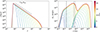 |
Fig. 1. Temporal evolution of the electron distribution Ne(γ) multiplied by γ (left panel) and of the emitted SSC spectra (right panel) during a particle acceleration episode for the parameters listed in Table 1. The colors indicate different times (in units of tacc; see the color bar). The dashed line in the left panel shows the model-predicted slope for the electron distribution. The vertical solid and dashed lines in the right panel indicate the characteristic NIR (2.2 μm) and X-ray (2–10 keV) frequencies, respectively. |
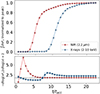 |
Fig. 2. Flux and photon index plotted as a function of time for the rising part of an NIR and X-ray flare. Top panel: NIR and X-ray light curves (normalized to their peak values) of the SSC model presented in Fig. 1. Bottom panel: Temporal evolution of the photon index at NIR and X-ray frequencies. For the latter case, the average value of the photon index in the 2–10 keV band is plotted. The error bar shows the standard deviation of the values in the 2–10 keV range. The horizontal dotted line marks the theoretical value of the photon index. In both panels, the markers are used to show the cadence of the numerical calculation (1 tcr). |
After the end of the acceleration episode, particles are left to cool and escape from the active region on the respective timescales (see also Sect. 2). Depending on the particle escape timescale, different decaying flare profiles can be obtained. This is illustrated in the top panel of Fig. 3, where we show results for two extreme cases: Particles escape on R/c, that is, on the shortest possible timescale from the flaring region after the end of the acceleration phase (solid lines), or they are not allowed to escape at all (dashed lines). In the latter case, the NIR flux decays on the cooling timescale of the radiating electrons, which is much longer than that of X-ray emitting electrons (see also Eq. (9)). Moreover, the X-ray profile is asymmetric in both cases, and the rise time is longer than the decay time of the flare because a plateau forms in the X-ray light curve. However, when the acceleration episode does not last long enough to lead to a saturation of the high-energy cutoff of the electron distribution, the X-ray flare will appear symmetric, as shown in the bottom panel of Fig. 3. Finally, the flare profiles at longer wavelengths are generally asymmetric, unless the particle escape timescale  is set to be comparable to the rise time.
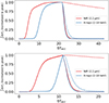 |
Fig. 3. Light curves of an NIR and X-ray flare for two different choices of the particle acceleration duration. Top panel: NIR and X-ray light curves for the same flare as in Figs. 1 and 2, but also accounting for the decay phase. We show the results for two choices of the particle escape timescale during the decay: |


In Appendix A we discuss how other model parameters, such as the initial Lorentz factor of electrons before their injection into the acceleration phase and the size of the active region, may affect the multiwavelength spectra of the flare. Moreover, we discuss the case of the energy-dependent acceleration/escape timescales and the impact of Doppler boosting on the shape of the light curves, which may arise due to the relative motion of the active region and the observer by considering an indicative trajectory.
3.2. Variable injection rate
In the previous section, we assumed that the injection rate of particles with γ0 was constant during the flare. To demonstrate the effects of variable injection of low-energy electrons into the flaring region, we constructed a red-noise time series for Q06 using the Python package colorednoise. This is shown by the dashed grey line in the left panel of Fig. 4. We also introduced two acceleration episodes that lasted two hours and one hour each, as indicated by the horizontal lines in the same figure. All other parameters were the same as those listed in Table 1. In the first acceleration episode, lasting about 20 R/c, the high-energy cutoff of the electron distribution approached γsat. In contrast, γmax in the second episode was limited by the shorter duration to lower values.
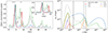 |
Fig. 4. Light curves and spectra of a nonthermal flare computed for a variable particle injection rate. Left panel: Light curves at different energies (500 GHz: green; NIR: red; X-rays: blue) computed for a variable injection rate Q0 that mimics red noise (dashed gray line). All other parameters are the same as in Table 1. Two episodes of acceleration are assumed to take place and are indicated by the horizontal bars. The time series in the left panel are normalized to their peak values, and a zoom in the first 10 h is shown in the inset plot. The light curves do not account for the background flux arising from the accretion flow. Right panel: SED snapshots of our model. For comparison, the quiescent emission model of Yuan et al. (2003) is also shown (dotted curve). An animation of the full temporal evolution of the broadband spectra can be found at this link. |
In Fig. 4 we present (normalized) light curves (left panel) and SED snapshots of the emission produced by nonthermal electrons in the flaring region. In the absence of acceleration, electrons with γ0 ∼ 500 produce ∼500 GHz photons (green line) in a region with a magnetic field of strength of ∼1 G, as shown in the first SED snapshot in the right panel (at 3 h). Hence, before the start of the first acceleration episode, no NIR (2.2 μm) emission is expected from the active region. Soon after the onset of the first acceleration episode, the NIR (red line) and X-ray (blue line) fluxes rise sharply, and the X-rays lag about ∼5tacc ∼ 0.8 h with respect to the NIR frequencies (see also Fig. 2). The amplitude of the flux variations in the X-rays is expected to be larger than in NIR frequencies. During the first acceleration episode, the flux at 500 GHz is suppressed and does not follow the injection rate profile because particles injected at γ0 are shifted to higher energies (see the inset plot in the left panel). In other words, the injected energy that would otherwise be radiated at 500 GHz is now channeled to higher frequencies. Interestingly, similar indications have been reported by Wielgus et al. (2022), who found spectral changes at 1.3 mm close to the peak time of an X-ray flare in Sgr A⋆ (see Fig. 6 in their paper). At the end of the acceleration phase, the NIR and X-ray fluxes decrease on a light-crossing timescale (because the electrons in this example escape from the region on the same timescale), while the 500 GHz flux increases (see also SEDs at 4 h and 5 h in the right panel).
The second acceleration episode is identified by a rapid decrease in the 500 GHz luminosity and the emergence of an NIR flare, which lacks an X-ray counterpart, however: Because this episode is shorter, particles injected with γ0 do not have enough time to reach a large enough Lorentz factor, and they emit X-rays via synchrotron radiation. Still, electrons at γ0 produce SSC radiation at a characteristic frequency νssc ≈ 1.7 × 10¹⁷ Hz (γ0/500)2(νsyn/500 GHz), which emerges in the X-rays for the chosen parameters. Therefore, enhancements in the X-ray luminosity that are not accompanied by NIR flares are also expected due to the stochastic changes in the electron injection rate (see, e.g., the SEDs in the right panel at 15 h). In general, the X-ray luminosity in this case is lower than the luminosity expected from a synchrotron flare caused by particle acceleration (compare the X-ray luminosities at ∼5 h and 15 h).
In Fig. 5 we plot the X-ray and NIR fluxes (normalized to their peak values) against the 500 GHz flux from the flaring region that tracks the variations in the injection rate. The colored markers indicate the flux evolution from the period of the first acceleration episode, lasting about 4 h. NIR and X-ray flares produced by an episode of particle acceleration that is followed by a particle cooling/escape phase form clockwise loops in this diagram. The later onset of the X-ray flare results in a smaller loop than for the NIR flare. Loops in flux-flux diagrams have long been sought for in AGN X-ray and TeV γ-ray flares (e.g. Mastichiadis & Moraitis 2008; Moraitis & Mastichiadis 2011) because they can provide a glimpse into the underlying particle acceleration process.
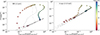 |
Fig. 5. Flux-flux diagram for the case presented in Fig. 4 (gray symbols). The colored symbols indicate the evolution during the first nonthermal flare shown in Fig. 4 (see also the color bar). All fluxes refer to the flaring region. |
4. Application to the 2014 NIR and X-ray flare
We considered the first simultaneous observations of X-ray and NIR emission of a very bright flare of Sgr A⋆, which occurred between 2014 August 30 and 31 (Ponti et al. 2017). We applied our model to four time windows identified by Ponti et al. (2017) in which simultaneous NIR and X-ray spectra could be constructed. These epochs, each one lasting 600 s, correspond to the pre-rise (IR1), rise (IR2), peak (IR3), and decay (IR4) of the flare. We reprocessed the XMM-Newton data using the same procedure as Ponti et al. (2017), but with the 2023 calibration files. The data are fully consistent with those reported in Ponti et al. (2017).
Having as guideline the analytical expressions in Sect. 2, we find physically motivated parameter values that can reproduce the general spectral and temporal properties of the observed flare. Our results, which were obtained for similar parameter values as in the default set used in the previous section (see Tables 1 and 2), are presented in Fig. 6. The model naturally explains the X-ray nondetection during IR1 because the highest-energy particles of the distribution have not yet reached high enough energies to emit in the X-rays. To reproduce the fast and slow decays of the X-ray and NIR flares, respectively, a longer escape timescale (12.5R/c) from the active region is required after the acceleration ceases to operate. While the fast decay of the X-ray flare is dictated by the synchrotron cooling timescale, the NIR decay timescale reflects the electron escape rate.
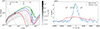 |
Fig. 6. Application of the model to the 2014 nonthermal flare from Sgr A⋆. Left panel: SED evolution during the 2014 bright flare of Sgr A⋆ (symbols). Snapshots of model spectra (every tcr is plotted with thin gray lines). The thick lines represent the average model spectra during the four observation time windows. Right panel: NIR and X-ray model light curves (solid lines) plotted against the data of the 2014 flare (symbols). After the peak time of the flare, the particles escape from the active region on a timescale 12.5 R/c. The data are adopted from Ponti et al. (2017). |
Model parameter values for the 2014 bright flare of Sgr A*.
In addition to the SED of the nonthermal flare, we show in Fig. 6 the spectrum of the accretion flow based on the model of Yuan et al. (2003). If the flare is produced in a compact region of the accretion flow (blob), it could be embedded in a photon bath produced by the hot electrons in the flow. These low-energy photons could provide external targets for inverse-Compton scattering by the electrons in the blob. The energy density of the submm quiescent photon field is usmm = Lsmm/(4πRsmm2c)≃6 × 10−3 Lsmm, 35.6(10RS/Rsmm)2 erg cm−3, where we used the peak luminosity of the submm bump as a proxy for the bolometric luminosity. The magnetic energy density of the blob producing the flare is uB ≃ 4 × 10⁻²(B/1G)2 erg cm−3. Since uB > usmm, inverse-Compton scattering in the submm quiescent photon field contributes significantly to the high-energy spectrum of the flare (and to the cooling of nonthermal electrons).
So far, no NIR and X-ray flare from Sgr A⋆ has been observed in very high energies (VHE; > 100 GeV). In Fig. 7 we show a zoom in the γ-ray spectra of our 2014 flare model. The cutoff of the SSC spectrum at the peak time of the X-ray flare (IR3) scratches the 30 min sensitivity curve7 of the Cherenkov Telescope Array Observatory (CTAO) South (Abdalla et al. 2021). CTAO South could place meaningful upper limits or even secure a detection of the VHE counterpart of bright X-ray flares from Sgr A⋆ in the future. We also overplot the 60 MeV to 500 GeV spectrum of the point source 4FGL J1745.6–2859, which was constructed using 10.5 years of Fermi-LAT data, and is thought to be associated with Sgr A⋆ (Cafardo et al. 2021). However, a GeV counterpart of the flare would remain undetectable by Fermi-LAT due to the small fluence (short duration of the flares).
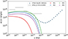 |
Fig. 7. Zoom in the γ-ray range of the model spectra computed for epochs IR1–IR4. The differential sensitivity curve of CTAO South for an observing time of 30 min is overplotted. The black lines indicate the 10.5 yr integrated Fermi-LAT spectrum for the γ-ray source 4FGL J1745.6-2859, which is associated with the Galactic center (Cafardo et al. 2021). |
5. Summary and discussion
We have presented a model for the production of NIR and X-ray flares motivated by multiwavelength observations of Sgr A⋆. The model invokes a phase of particle energization that is followed by a period of particle cooling and escape from the active region. We first provided an analytical description of the model that highlighted the role of key physical parameters and their relation to flare observables. We then presented numerical results for the flare SED and light curves and applied our model to the 2014NIR and X-ray flare of Sgr A⋆.
There are several differences between our model and the standard synchrotron cooling model for Sgr A⋆ flares regarding the physical conditions in the flaring region that are worth mentioning. For NIR and X-ray flares with similar characteristics as those of the 2014 flare, our model predicts much weaker magnetic fields (∼1 G) and more extended flaring regions (R ∼ (5 − 10) RS) than the synchrotron cooling model (Ponti et al. 2017; GRAVITY Collaboration 2021). An attempt to consider smaller radii to explain the same NIR and X-ray luminosity would result in a flare with strong Compton dominance, as demonstrated in Appendix A.1, which would contradict the soft X-ray spectrum. Moreover, the spectral break between the NIR and X-ray energy ranges in our model is not related to the cooling of particles, but to the onset of the exponential cutoff of the synchrotron spectrum. The evolution of this spectral cutoff, νmax ∝ Bγmax2, is also very distinct: It increases exponentially during the rise of the flare, namely νmax ∝ e2t/tacc (see Eq. (4)), and decreases during the decay as a power law with time, νmax ∝ (1 + bsγsat(t − tpk))−2. Last but not least, our model predicts a lag between the onset of the X-ray and NIR flares (see, e.g., Fig. 3), which can be directly linked to the particle acceleration timescale. In contrast, the flux in both energy bands evolves simultaneously in the synchrotron cooling-break model.
In our framework, NIR flares without an X-ray counterpart are naturally expected when the duration of an acceleration episode is shorter than the time needed to accelerate particles to sufficiently high energies (see Fig. 4). Using analytical expressions from Sect. 2, we can estimate the number ratio of NIR flares with and without X-ray emission predicted by our model. Let γX = γsat be the Lorentz factor of electrons emitting X-ray photons of energy ϵX. Using Eqs. (4) and (8), we find that  . Here, tacc = 2tesc(sph, NIR − 1), where sph, NIR is the NIR to X-ray photon index. Similarly, the Lorentz factor of electrons emitting at NIR can be written as
  . The time needed for particles with an initial Lorentz factor γ0 to reach γX, γNIR can be obtained from Eq. (11), namely tX, NIR = taccln[ξ/(1−ξ)(γX, NIR/γ0−1)]. The ratio of the two timescales is tX/tNIR ∼ 1.6 for the parameters used in Fig. 2, but it does not depend strongly on the model parameters because of the logarithmic term. Assuming that the duration of the particle acceleration phase, T, follows a power-law distribution, dN/dT ∝ T−a, a > 1, we can estimate the number of NIR without an X-ray counterpart as
  . The number of flares expected in both NIR and X-rays is
  . Therefore, the number ratio of NIR and X-ray flares to NIR flares is NNIR/X/NNIR = (tX/tNIR)−a + 1/[1 − (tX/tNIR)−a + 1], which ranges between 0.2 and 0.8 for a = 5 and a = 3, respectively. These estimates are optimistic because they do not account for instrumental effects and observational biases.
So far, we have remained agnostic to the nature of the acceleration mechanism. GRMHD simulations of accretion onto black holes have shown the formation of current sheets (in the disk and in the boundary between the disk and the funnel) that are potential sites of energy dissipation and particle acceleration through magnetic reconnection (e.g. Ball et al. 2018a; Nathanail et al. 2020, 2022; Ripperda et al. 2022). The properties of the accelerated particles (e.g., power-law slope and maximum energy) depend on local plasma properties, such as the magnetization σ (defined as twice the ratio of the magnetic energy density to the plasma enthalpy density), the plasma-β parameter (defined as the ratio of thermal and magnetic pressures), and the plasma composition (e.g. Sironi & Spitkovsky 2014; Ball et al. 2018b; Werner et al. 2018; Petropoulou et al. 2019). During reconnection, particles may gain energy by the reconnection electric field Erec ∼ βrecB on a timescale tacc ≈ meγc2/(eβrecBc), where βrec ∼ 0.1 is the reconnection rate and B is the strength of the reconnecting magnetic field (for 3D simulations, see also Zhang et al. 2021, 2023). The saturation Lorentz factor in this scenario can be estimated by balancing the synchrotron cooling and acceleration timescales, namely  . Electrons with γsat therefore radiate synchrotron photons of ∼15.8 MeV energy, regardless of the magnetic field strength (synchrotron burnoff limit, de Jager et al. 1996). Because there is evidence of a spectral cutoff at tens of keV in X-rays flares from Sgr A⋆ (see, e.g., Fig. 6), we can conclude that the maximum electron energy cannot be limited by radiation. It could instead be limited by the size ℓ of the accelerator (Hillas limit, Hillas 1984), which can be estimated as
  . To compensate for the small emitting volume while accounting for the observed luminosity of flares, a large number of nonthermal electrons would be needed. The high-electron compactness of the emitting region would lead to Compton-dominated SEDs, which is in contrast to observations (see, e.g., Fig. A.1). Moreover, the acceleration timescale is very short compared to the typical duration of X-ray flares for typical magnetic field strengths in the inner accretion flow, for example, tacc ≈ 10−6 (γ/100)(B/1G)−1 (RS/c). As a result, the acceleration would be instantaneous, and neither the rise time of the X-ray flare nor a lag between NIR and X-ray flares could be explained by tacc in this case. Therefore, if direct acceleration by the reconnection electric field in macroscopic current sheets energizes particles during flares in Sgr A⋆, then models considering the injection of preaccelerated particles into a radiation zone in which particles cool and/or escape would be appropriate for the flare description (e.g. Dodds-Eden et al. 2010; Ball et al. 2021; Lin & Yuan 2024; Dimitropoulos et al. 2024).
Alternatively, particles can accelerate in environments of magnetized turbulence by the reconnecting electric field at transient current sheets and/or stochastically through multiple scatterings by turbulent fluctuations. Recently, particle-in-cell (PIC) simulations of magnetized turbulence have demonstrated from first principles the formation of power-law particle distributions (Zhdankin et al. 2017, 2018; Comisso & Sironi 2018). By analyzing particle trajectories in PIC simulations, Comisso & Sironi (2019) showed that low-energy particles typically experience a small energy gain at the current sheets before they are injected into a diffusive acceleration process. Interestingly, the authors found that the relevant acceleration timescale is independent of energy (nongyroresonant scatterings; see also Wong et al. 2020) and can be expressed in terms of the turbulence driving-scale ℓt and of the plasma magnetization (defined with respect to the turbulent component of the magnetic field) σt, as tacc ≈ (10/σtur)ℓt/c (see also Fiorillo et al. 2024). Writing ℓt as a fraction η of the source size R, we find that tacc ≈ tcr(η/0.1)(σt/1)−1, which is comparable to the value used to model the 2014 NIR and X-ray flare (see Table 2). Furthermore, the synchrotron-limited maximum particle energy is also similar to the energy found in our generic model (see Sect. 2). Despite these promising similarities, a more detailed investigation of the nonresonant acceleration-radiation model would require us to solve the time-dependent kinetic equation of Eq. (1) after replacing the second term with a diffusive one,  . The new PDE admits stationary solutions of the form Ne ∝ γ−1 (power law) for γ ≪ γsat, and Ne ∝ γ2 for γ ≲ γsat (pile up) (for more details, see Fiorillo et al. 2024). Compared to the stationary solution of our generic model, the main difference is the formation of a pile-up, which may result in interesting observable features.
6. Conclusions
We have introduced a generic acceleration-radiation model for nonthermal flares in Sgr A⋆. According to the model, particles are energized in an active region with a size of a few Schwarzschild radii on an energy-independent acceleration timescale while experiencing mainly synchrotron losses. Particles physically escape this region on a timescale comparable to their acceleration timescale. The emitted synchrotron spectra are power laws, with a photon index determined by the ratio of the acceleration and escape timescales, followed by an exponential cutoff. This occurs at the synchrotron photon energy emitted by particles with the maximum Lorentz factor (where the energy loss and energy gain rates become equal). The model predicts an increases in NIR flux before the onset of the X-ray flare. This time difference as well as the rise time of the X-ray flare are multiples of the particle acceleration timescale. Our generic model for NIR and X-ray flares favors an interpretation of diffusive (nonresonant) particle acceleration in magnetized turbulence. This requires a more detailed investigation.
Data availability
Movie associated with Fig. 4 is available at https://www.aanda.org
The Schwarzschild radius of Sgr A⋆ is RS = 2GM/c2 ≃ 1.2 × 1012 cm, for a black hole mass of 4.3 × 10⁶ M⊙ (GRAVITY Collaboration 2019).
We discuss the effects of energy-dependent timescales in Appendix A.3.
The approximate relation is found by integrating Eq. (2) over γ, ignoring the term in the parentheses, and using γ0 ≪ γsat.
Particle and photon energies are normalized to mec2.
This should not to be confused with the compactness, which is usually defined with respect to the bolometric power in nonthermal electrons.
The time resolution of the series is R/c.
The adopted exposure is comparable to the full width at half maximum of the X-ray flare (see Fig. 6).
We note a typo in Eq. (A5) of Kirk et al. (1998), which is missing a square root from the square brackets. We also note that Kirk et al. (1998) use the symbol γmax to denote the asymptotic value of the Lorentz factor, labeled as γsat here.
The corresponding expression in Kirk et al. (1998) (Eq. A6) is missing the factor γsat multiplying the logarithmic term.
Acknowledgments
M.P. acknowledges support from the Hellenic Foundation for Research and Innovation (H.F.R.I.) under the “2nd call for H.F.R.I. Research Projects to support Faculty members and Researchers” through the project UNTRAPHOB (Project ID 3013). This work is based on observations obtained with XMM-Newton, an ESA science mission with instruments and contributions directly funded by ESA Member States and NASA. G.P. acknowledges financial support from the European Research Council (ERC) under the European Union’s Horizon 2020 research and innovation program HotMilk (grant agreement No. 865637), support from Bando per il Finanziamento della Ricerca Fondamentale 2022 dell’Istituto Nazionale di Astrofisica (INAF): GO Large program and from the Framework per l’Attrazione e il Rafforzamento delle Eccellenze (FARE) per la ricerca in Italia (R20L5S39T9).
References
- Abdalla, H., Abe, H., Acero, F., et al. 2021, JCAP, 2021, 048 [CrossRef] [Google Scholar]
- Andrés, A., van den Eijnden, J., Degenaar, N., et al. 2022, MNRAS, 510, 2851 [CrossRef] [Google Scholar]
- Baganoff, F. K., Maeda, Y., Morris, M., et al. 2003, ApJ, 591, 891 [Google Scholar]
- Ball, D., Özel, F., Psaltis, D., Chan, C.-K., & Sironi, L. 2018a, ApJ, 853, 184 [NASA ADS] [CrossRef] [Google Scholar]
- Ball, D., Sironi, L., & Özel, F. 2018b, ApJ, 862, 80 [Google Scholar]
- Ball, D., Özel, F., Christian, P., Chan, C.-K., & Psaltis, D. 2021, ApJ, 917, 8 [NASA ADS] [CrossRef] [Google Scholar]
- Bouffard, É., Haggard, D., Nowak, M. A., et al. 2019, ApJ, 884, 148 [NASA ADS] [CrossRef] [Google Scholar]
- Cafardo, F., Nemmen, R., & Fermi, L. C. 2021, ApJ, 918, 30 [NASA ADS] [CrossRef] [Google Scholar]
- Comisso, L., & Sironi, L. 2018, Phys. Rev. Lett., 121, 255101 [NASA ADS] [CrossRef] [Google Scholar]
- Comisso, L., & Sironi, L. 2019, ApJ, 886, 122 [Google Scholar]
- Cuadra, J., Nayakshin, S., Springel, V., & Di Matteo, T. 2006, MNRAS, 366, 358 [NASA ADS] [CrossRef] [Google Scholar]
- Cuadra, J., Nayakshin, S., & Martins, F. 2008, MNRAS, 383, 458 [NASA ADS] [Google Scholar]
- de Jager, O. C., Harding, A. K., Michelson, P. F., et al. 1996, ApJ, 457, 253 [Google Scholar]
- Degenaar, N., Miller, J. M., Kennea, J., et al. 2013, ApJ, 769, 155 [NASA ADS] [CrossRef] [Google Scholar]
- Dibi, S., Markoff, S., Belmont, R., et al. 2014, MNRAS, 441, 1005 [NASA ADS] [CrossRef] [Google Scholar]
- Dimitrakoudis, S., Mastichiadis, A., Protheroe, R. J., & Reimer, A. 2012, A&A, 546, A120 [NASA ADS] [CrossRef] [EDP Sciences] [Google Scholar]
- Dimitropoulos, I., Nathanail, A., Petropoulou, M., & Contopoulos, I. 2024, A&A, submitted [Google Scholar]
- Do, T., Ghez, A. M., Morris, M. R., et al. 2009, ApJ, 691, 1021 [NASA ADS] [CrossRef] [Google Scholar]
- Dodds-Eden, K., Sharma, P., Quataert, E., et al. 2010, ApJ, 725, 450 [NASA ADS] [CrossRef] [Google Scholar]
- Eckart, A., Baganoff, F. K., Morris, M., et al. 2004, A&A, 427, 1 [NASA ADS] [CrossRef] [EDP Sciences] [Google Scholar]
- Eckart, A., Schödel, R., García-Marín, M., et al. 2008, A&A, 492, 337 [CrossRef] [EDP Sciences] [Google Scholar]
- EHT Collaboration 2022, ApJ, 930, L16 [NASA ADS] [CrossRef] [Google Scholar]
- Fiorillo, D. F. G., Comisso, L., Peretti, E., Petropoulou, M., & Sironi, L. 2024, ApJ, 974, 75 [NASA ADS] [CrossRef] [Google Scholar]
- Genzel, R., Eisenhauer, F., & Gillessen, S. 2010, Rev. Mod. Phys., 82, 3121 [Google Scholar]
- GRAVITY Collaboration (Abuter, R., et al.) 2018, A&A, 618, L10 [NASA ADS] [CrossRef] [EDP Sciences] [Google Scholar]
- GRAVITY Collaboration (Abuter, R., et al.) 2019, A&A, 625, L10 [NASA ADS] [CrossRef] [EDP Sciences] [Google Scholar]
- GRAVITY Collaboration (Bauböck, M., et al.) 2020, A&A, 635, A143 [CrossRef] [EDP Sciences] [Google Scholar]
- GRAVITY Collaboration (Abuter, R., et al.) 2021, A&A, 654, A22 [NASA ADS] [CrossRef] [EDP Sciences] [Google Scholar]
- Gutiérrez, E. M., Nemmen, R., & Cafardo, F. 2020, ApJ, 891, L36 [Google Scholar]
- Hillas, A. M. 1984, ARA&A, 22, 425 [Google Scholar]
- Hornstein, S. D., Matthews, K., Ghez, A. M., et al. 2007, ApJ, 667, 900 [NASA ADS] [CrossRef] [Google Scholar]
- Kirk, J. G., Rieger, F. M., & Mastichiadis, A. 1998, A&A, 333, 452 [NASA ADS] [Google Scholar]
- Lin, X., & Yuan, F. 2024, MNRAS, 531, 3136 [NASA ADS] [CrossRef] [Google Scholar]
- Loeb, A., & Waxman, E. 2007, JCAP, 2007, 011 [NASA ADS] [CrossRef] [Google Scholar]
- Markoff, S., Falcke, H., Yuan, F., & Biermann, P. L. 2001, A&A, 379, L13 [NASA ADS] [CrossRef] [EDP Sciences] [Google Scholar]
- Marrone, D. P., Baganoff, F. K., Morris, M. R., et al. 2008, ApJ, 682, 373 [Google Scholar]
- Mastichiadis, A., & Moraitis, K. 2008, A&A, 491, L37 [NASA ADS] [CrossRef] [EDP Sciences] [Google Scholar]
- Melia, F. 1992, ApJ, 387, L25 [NASA ADS] [CrossRef] [Google Scholar]
- Moraitis, K., & Mastichiadis, A. 2011, A&A, 525, A40 [NASA ADS] [CrossRef] [EDP Sciences] [Google Scholar]
- Mossoux, E., & Grosso, N. 2017, A&A, 604, A85 [NASA ADS] [CrossRef] [EDP Sciences] [Google Scholar]
- Mossoux, E., Grosso, N., Bushouse, H., et al. 2016, A&A, 589, A116 [NASA ADS] [CrossRef] [EDP Sciences] [Google Scholar]
- Nathanail, A., Fromm, C. M., Porth, O., et al. 2020, MNRAS, 495, 1549 [Google Scholar]
- Nathanail, A., Dhang, P., & Fromm, C. M. 2022, MNRAS, 513, 5204 [NASA ADS] [CrossRef] [Google Scholar]
- Neilsen, J., Nowak, M. A., Gammie, C., et al. 2013, ApJ, 774, 42 [NASA ADS] [CrossRef] [Google Scholar]
- Neilsen, J., Markoff, S., Nowak, M. A., et al. 2015, ApJ, 799, 199 [NASA ADS] [CrossRef] [Google Scholar]
- Petropoulou, M., Sironi, L., Spitkovsky, A., & Giannios, D. 2019, ApJ, 880, 37 [Google Scholar]
- Ponti, G., De Marco, B., Morris, M. R., et al. 2015, MNRAS, 454, 1525 [NASA ADS] [CrossRef] [Google Scholar]
- Ponti, G., George, E., Scaringi, S., et al. 2017, MNRAS, 468, 2447 [NASA ADS] [CrossRef] [Google Scholar]
- Quataert, E. 2002, ApJ, 575, 855 [NASA ADS] [CrossRef] [Google Scholar]
- Ripperda, B., Liska, M., Chatterjee, K., et al. 2022, ApJ, 924, L32 [NASA ADS] [CrossRef] [Google Scholar]
- Rybicki, G. B., & Lightman, A. P. 1986, Radiative Processes in Astrophysics (Wiley-VCH) [Google Scholar]
- Sironi, L., & Spitkovsky, A. 2014, ApJ, 783, L21 [NASA ADS] [CrossRef] [Google Scholar]
- Trap, G., Goldwurm, A., Dodds-Eden, K., et al. 2011, A&A, 528, A140 [NASA ADS] [CrossRef] [EDP Sciences] [Google Scholar]
- Werner, G. R., Uzdensky, D. A., Begelman, M. C., Cerutti, B., & Nalewajko, K. 2018, MNRAS, 473, 4840 [Google Scholar]
- Wielgus, M., Marchili, N., Martí-Vidal, I., et al. 2022, ApJ, 930, L19 [NASA ADS] [CrossRef] [Google Scholar]
- Witzel, G., Eckart, A., Bremer, M., et al. 2012, ApJS, 203, 18 [NASA ADS] [CrossRef] [Google Scholar]
- Witzel, G., Martinez, G., Hora, J., et al. 2018, ApJ, 863, 15 [NASA ADS] [CrossRef] [Google Scholar]
- Witzel, G., Martinez, G., Willner, S. P., et al. 2021, ApJ, 917, 73 [NASA ADS] [CrossRef] [Google Scholar]
- Wong, K., Zhdankin, V., Uzdensky, D. A., Werner, G. R., & Begelman, M. C. 2020, ApJ, 893, L7 [NASA ADS] [CrossRef] [Google Scholar]
- Xu, Y.-D., Narayan, R., Quataert, E., Yuan, F., & Baganoff, F. K. 2006, ApJ, 640, 319 [NASA ADS] [CrossRef] [Google Scholar]
- Yuan, Q., & Wang, Q. D. 2016, MNRAS, 456, 1438 [CrossRef] [Google Scholar]
- Yuan, F., Quataert, E., & Narayan, R. 2003, ApJ, 598, 301 [Google Scholar]
- Yusef-Zadeh, F., Bushouse, H., Dowell, C. D., et al. 2006, ApJ, 644, 198 [NASA ADS] [CrossRef] [Google Scholar]
- Yusef-Zadeh, F., Wardle, M., Heinke, C., et al. 2008, ApJ, 682, 361 [NASA ADS] [CrossRef] [Google Scholar]
- Zhang, H., Sironi, L., & Giannios, D. 2021, ApJ, 922, 261 [NASA ADS] [CrossRef] [Google Scholar]
- Zhang, H., Sironi, L., Giannios, D., & Petropoulou, M. 2023, ApJ, 956, L36 [NASA ADS] [CrossRef] [Google Scholar]
- Zhdankin, V., Werner, G. R., Uzdensky, D. A., & Begelman, M. C. 2017, Phys. Rev. Lett., 118, 055103 [NASA ADS] [CrossRef] [Google Scholar]
- Zhdankin, V., Uzdensky, D. A., Werner, G. R., & Begelman, M. C. 2018, ApJ, 867, L18 [NASA ADS] [CrossRef] [Google Scholar]
Appendix A: Effects of model parameters
In this section we demonstrate the effect of model parameters, like the initial Lorentz factor of electrons before their injection into the acceleration phase, and the size of the active region, on the multi-wavelength spectra of the flare. We also discuss a scenario with energy-dependent particle timescales, and investigate how the relative motion of the active region and the observer can affect the shape of the light curves.
A.1. Size of flaring region
In the acceleration-radiation model for flares the ratio tesc/tacc, which determines the asymptotic power-law slope of the particle distribution, can be inferred by the observed photon index at NIR frequencies. Given the latter, a smaller flaring region would imply shorter tacc as long as tesc = R/c. Because the acceleration would become faster, a stronger magnetic field,  , would be needed to stop the acceleration at a maximum electron energy that will be sufficient to produce X-ray synchrotron photons – see Eq. (8). Moreover, if the electron injection compactness is fixed, then the injection rate of electrons at γ0 is Q0 ∝ R according to Eq. (15). Therefore, the synchrotron luminosity of a flare (at a fixed frequency ν) produced from a smaller region would decrease as νLsyn(ν)∝R4/3 − tacc/(3tesc) – see Eq. (5).
These effects are illustrated in Fig. A.1 where we plot (solid lines) the electron distributions (top panel) and photon spectra (bottom panel) at t = 10 tacc for R = 10, 1, 0.1 RS. In all cases, the magnetic field B has been adjusted accordingly as to produce a synchrotron cutoff energy falling in the 2-10 keV range (see inset legend). Meanwhile, the dynamic range of the power-law synchrotron spectrum decreases as B gets stronger and γ0 remains the same. Moreover, the synchrotron luminosity decreases by a factor of ∼0.15 as the radius decreases by a factor of 10, in agreement with Eq. (5) – see also scaling relation at the end of the previous paragraph. To achieve the same synchrotron luminosity in all three cases, the injection rate Q0 would have to increase accordingly. This is exemplified for the case with R = 0.1RS (see dashed and dotted green lines). As the particle density increases, SSC cooling becomes progressively more important than synchrotron, thus pushing the synchrotron cutoff energy below the X-ray band, and increasing the luminosity of the SSC component (i.e. Compton-dominated flare).
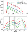 |
Fig. A.1. Effects of the flaring region size on particle and photon spectra of a nonthermal flare. Top panel: Electron distribution Ne(γ) multiplied by γ at t = 10 tacc for different radii and magnetic field strengths of the flaring region (see inset legend) and the same electron compactness ℓe (see Table 1). For R = 0.1 RS we also show results for 5ℓe (dashed line) and 25ℓe. Bottom panel: SSC spectra produced by the electron distributions shown on the left panel. |
Using the analytical expressions in Sect. 2 we can also predict the radiative output of flaring regions with the same magnetic field but different radii. For example, if B is constant and Q0 ∝ R, then the synchrotron luminosity of a flare (at a fixed frequency ν) would scale as νLsyn(ν)∝R2, while the cutoff synchrotron frequency would scale as  . Hence, smaller regions would produce less luminous NIR and X-ray flares, with synchrotron spectra extending beyond the X-ray band. Alternatively, if one considers that the power injected into the electrons with γ0 is the same regardless of the flaring region size, i.e. Q0 does not depend on R, the luminosity of the flare would scale as νLsyn(ν)∝R.
Summarizing, most model parameters (tacc/tesc, B, R) can be constrained if the photon index, the luminosity and spectrum of the NIR and X-ray flare are known.
A.2. Initial electron Lorentz factor
To illustrate the effects of the Lorentz factor of electrons when injected in the acceleration region, we present in Fig. A.2 results for three values of γ0 (see inset legend). We also adjust the injection compactness ℓe in each case so that the number of electrons at the cutoff of the distribution remains the same, thus producing the same level of X-ray emission, as shown on the bottom panel of the figure. Since particles are accelerated from different values of γ0, the time needed for the cutoff Lorentz factor of the distribution to reach its saturation value increases with decreasing γ0. Therefore, the choice of γ0 affects the time delay between the onset of the NIR and X-ray flares. The broadband photon spectra are similar in all cases, with some differences appearing in the low-end of the synchrotron spectrum and the peak of the SSC spectrum. The synchrotron spectrum becomes self-absorbed around 10 GHz for lower values of γ0 since the number of low-energy electrons increases, as shown in the top panel.
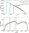 |
Fig. A.2. Effects of the minimum electron Lorentz factor on particle and photon spectra of a nonthermal flare. Top panel: Electron distribution Ne(γ) multiplied by γ for different values of the initial Lorentz factor γ0 and electron compactness ℓe (see inset legend). All other parameters are the same as in Table 1. Bottom panel: SSC spectra produced by the electron distributions shown on the left panel. The snapshots shown in both panels are computed at t = 11tacc, 14.5tacc, 17tacc for γ0 = 103.5, 102.7 and 100.7 respectively. |
A.3. Energy-dependent timescales
An important assumption made in our generic model is that both acceleration and escape timescales are constant (see Sect. 2), but more generally they can depend on the particle energy (or Lorentz factor). To exemplify the effects of the energy-dependent timescales, we adopt tacc = ta0γ, tesc = te0γ, and discuss the main differences with respect to our generic model.
When tacc and tesc have the same dependence on γ, there is an analytical solution for the particle distribution (Kirk et al. 1998), which reads8
![Mathematical equation: $$ \begin{aligned} N_e(\gamma ,t) = \frac{Q_0t_{a0} \gamma _{sat}^2}{(\gamma _{sat}^2-\gamma ^2)} \left[\frac{\gamma }{\gamma _{0}}\sqrt{\frac{\gamma _{sat}^2-\gamma _0^2}{\gamma _{sat}^2-\gamma ^2}}\right]^{-\frac{t_{a0}}{t_{e0}}}\Theta [t-\tau (\gamma )], \end{aligned} $$](/articles/aa/full_html/2024/11/aa52069-24/aa52069-24-eq31.gif) (A.1)
(A.1)
where γsat is the saturation Lorentz factor given by,
 (A.2)
(A.2)
and τ is given by9
![Mathematical equation: $$ \begin{aligned} \tau (\gamma ) = \frac{t_{a0}\gamma _{sat}}{2}\ln \left[\frac{(\gamma _{sat}+\gamma )(\gamma _{sat}-\gamma _{0})}{(\gamma _{sat}-\gamma )(\gamma _{sat}+\gamma _0)}\right]. \end{aligned} $$](/articles/aa/full_html/2024/11/aa52069-24/aa52069-24-eq33.gif) (A.3)
(A.3)
For γ ≪ γsat the particle distribution is a power law with slope s = ta0/te0, which is harder by 1 compared to the power-law spectrum obtained for constant timescales (see Eq. 2). The photon index of the emitted synchrotron spectrum is sph = (1 + ta0/te0)/2, and differs accordingly by 1/2 compared to the value given by Eq. 7.
The condition imposed by the step function in Eq. A.1 yields the time evolution of the high-energy cutoff of the particle distribution,
 (A.4)
(A.4)
where the approximation holds when γsat ≫ γ0.
To better illustrate the differences with the high-energy cutoff evolution given by Eq. 4, we plot in Fig. A.3γmax(t) for a constant acceleration timescale (red curve) and an acceleration timescale scaling linearly with particle energy (blue curves). For the latter case, we show results for ta0 = 0.15 tcr/γ0, B = 0.08 G (solid line) and ta0 = 0.0015 tcr/γ0, B = 0.8 G (dashed line), while ta0/te0 = 1.5 (where tcr = R/c). All other parameters are the same as in Table 1. For the selected parameter values, the saturation Lorentz factor is similar in all three cases, but the gradient of the γmax(t) curve is smaller when tacc ∝ γ. By appropriately choosing ta0 and B one controls γsat and the time needed to reach this value. These choices then map to the observed maximal synchrotron photon energy, ϵ ∝ Bγsat2, and the rise time of the light curve at that energy.
Using Eq. A.2 we can estimate the magnetic field strength needed to radiate synchrotron photons at a known photon energy ϵX by electrons with Lorentz factor γsat,
 (A.5)
(A.5)
The numerical value above was obtained for ta0/te0 = 1.5, ta0 = 0.15 tcr/γ0 ≃ 0.08 s, γ0 = 102.7, and R = 9.5RS. Unless the acceleration timescale is much faster than the photon crossing timescale (i.e., ta0γ0 ≪ tcr; see also blue dashed line in Fig. A.3), X-ray emitting electrons have to gyrate in ∼mG magnetic fields. Such values are disfavored by modeling of the sub-mm emission of Sgr A⋆ with synchrotron radiation of quasi-thermal electrons, which yields magnetic field strengths of ∼10 G in the inner accretion flow (see e.g. Genzel et al. 2010; EHT Collaboration 2022). Moreover, the energy density of nonthermal electrons in the blob,
 (A.6)
(A.6)
is many orders of magnitude larger than the magnetic energy density for mG fields, uB = B2/(8π), resulting in SSC-dominated photon spectra and electron cooling (see also Appendix A.1). In conclusion, a flare model for Sgr A⋆ with tacc = ta0γ and tesc = te0γ would require ta0, te0 ≪ tcr.
A.4. Doppler boosting
Astrometric observations performed by the Gravity interferometer during NIR flares have revealed that the NIR emitting region moves along loop trajectories with a projected radius on the plane of the sky of of ∼(6 − 10)⋅Rg (GRAVITY Collaboration 2018, 2020). Here, Rg = RS/2 is the gravitational radius of the black hole. Some interpretations of these observations include a compact region in the accretion flow (hot spot) moving on a circular orbit at a radius ∼9Rg around the black hole (GRAVITY Collaboration 2020) or a compact region (blob/plasmoid) orbiting the funnel region of the accreting black-hole system (Ball et al. 2021; Lin & Yuan 2024). Such structures, which are the result of magnetic reconnection, have been identified in general-relativistic magnetohydrodynamic (GRMHD) simulations (Nathanail et al. 2022; Ripperda et al. 2022; Lin & Yuan 2024).
To examine the effects of Doppler boosting on the light curves expected in our baseline model (see Fig. 3) arising from the relative motion of the emitting region and a distant observer, we adopt the scenario described in Ball et al. (2021). We assume that the flaring region is a blob that moves on a conical spiral trajectory. The equations of motion for the blob (in spherical coordinates) are:
 (A.7)
(A.7)
 (A.8)
(A.8)
 (A.9)
(A.9)
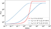 |
Fig. A.3. Time evolution of the particle distribution high-energy cutoff computed for constant (red curve) and energy-dependent (blue curves) acceleration timescales according to Eqs. 4 and A.4 respectively. For the parameters used, see inset legend. |
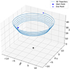 |
Fig. A.4. Blob trajectory computed for a period of 1300 Rg/c ≈ 68R/c where the blob radius is R ≈ 9.5RS. For the initial conditions, see text. |
where τ = ct/Rg, r = R/Rg, and υr is in units of c. The initial conditions are indicated by the subscript 0. The azimuthal velocity of the blob is given by  . The Doppler factor of the blob is then defined as:
 (A.10)
where Γb = (1 − υb2(τ))−1/2 , υb = (υr2 + υϕ2)1/2 is the blob velocity (in units of c), and nobs is a unit vector indicating the observer’s location. The photon frequency and integrated luminosities (between ν1 and ν2) as measured by a distant observer are then given by νobs = δν, and Lobs = δ4∫ν1ν2dνLν, while the time interval between the arrival of two photons in the observer’s frame is dτobs = dτ/δ(τ).
We adopt the initial conditions presented in Table 1 of Ball et al. (2021): r0 = 36, υr = 0.01, υϕ0 = 0.41, ϕ0 = 200o, θ0 = 15o, θobs = 168o and ϕobs = 90o. We vary ϕ0, υϕ0 and vr to illustrate their impact on the light curve shape. Throughout our calculations we assume that the conditions in the blob, such as B and R do not change with time, and are the same as those in listed in Table 1. We do not account for gravitational redshift and lensing. Our results are presented in Figs. A.5-A.10. Generally, Doppler boosting (or deboosting) of the emitted radiation by the blob produces multi-peaked light curves, thus increasing the complexity of the flare profiles in the baseline model.
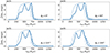 |
Fig. A.5. X-ray (2-10 keV) light curves (thick lines) computed for a blob moving on a conical spiral trajectory, starting from different initial azimuth angles (see inset legends). The observer is located at θobs = 168o in the y − z plane – see also Fig. A.4. Thin lines show the light curves without the Doppler boosting effects, as in Fig. 3. |
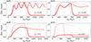 |
Fig. A.10. Same as in Fig. A.6 but for different radial blob velocities. |
All Tables
All Figures
|
Fig. 1. Temporal evolution of the electron distribution Ne(γ) multiplied by γ (left panel) and of the emitted SSC spectra (right panel) during a particle acceleration episode for the parameters listed in Table 1. The colors indicate different times (in units of tacc; see the color bar). The dashed line in the left panel shows the model-predicted slope for the electron distribution. The vertical solid and dashed lines in the right panel indicate the characteristic NIR (2.2 μm) and X-ray (2–10 keV) frequencies, respectively. |
| In the text | |
|
Fig. 2. Flux and photon index plotted as a function of time for the rising part of an NIR and X-ray flare. Top panel: NIR and X-ray light curves (normalized to their peak values) of the SSC model presented in Fig. 1. Bottom panel: Temporal evolution of the photon index at NIR and X-ray frequencies. For the latter case, the average value of the photon index in the 2–10 keV band is plotted. The error bar shows the standard deviation of the values in the 2–10 keV range. The horizontal dotted line marks the theoretical value of the photon index. In both panels, the markers are used to show the cadence of the numerical calculation (1 tcr). |
| In the text | |
|
Fig. 3. Light curves of an NIR and X-ray flare for two different choices of the particle acceleration duration. Top panel: NIR and X-ray light curves for the same flare as in Figs. 1 and 2, but also accounting for the decay phase. We show the results for two choices of the particle escape timescale during the decay: |
| In the text | |
|
Fig. 4. Light curves and spectra of a nonthermal flare computed for a variable particle injection rate. Left panel: Light curves at different energies (500 GHz: green; NIR: red; X-rays: blue) computed for a variable injection rate Q0 that mimics red noise (dashed gray line). All other parameters are the same as in Table 1. Two episodes of acceleration are assumed to take place and are indicated by the horizontal bars. The time series in the left panel are normalized to their peak values, and a zoom in the first 10 h is shown in the inset plot. The light curves do not account for the background flux arising from the accretion flow. Right panel: SED snapshots of our model. For comparison, the quiescent emission model of Yuan et al. (2003) is also shown (dotted curve). An animation of the full temporal evolution of the broadband spectra can be found at this link. |
| In the text | |
|
Fig. 5. Flux-flux diagram for the case presented in Fig. 4 (gray symbols). The colored symbols indicate the evolution during the first nonthermal flare shown in Fig. 4 (see also the color bar). All fluxes refer to the flaring region. |
| In the text | |
|
Fig. 6. Application of the model to the 2014 nonthermal flare from Sgr A⋆. Left panel: SED evolution during the 2014 bright flare of Sgr A⋆ (symbols). Snapshots of model spectra (every tcr is plotted with thin gray lines). The thick lines represent the average model spectra during the four observation time windows. Right panel: NIR and X-ray model light curves (solid lines) plotted against the data of the 2014 flare (symbols). After the peak time of the flare, the particles escape from the active region on a timescale 12.5 R/c. The data are adopted from Ponti et al. (2017). |
| In the text | |
|
Fig. 7. Zoom in the γ-ray range of the model spectra computed for epochs IR1–IR4. The differential sensitivity curve of CTAO South for an observing time of 30 min is overplotted. The black lines indicate the 10.5 yr integrated Fermi-LAT spectrum for the γ-ray source 4FGL J1745.6-2859, which is associated with the Galactic center (Cafardo et al. 2021). |
| In the text | |
|
Fig. A.1. Effects of the flaring region size on particle and photon spectra of a nonthermal flare. Top panel: Electron distribution Ne(γ) multiplied by γ at t = 10 tacc for different radii and magnetic field strengths of the flaring region (see inset legend) and the same electron compactness ℓe (see Table 1). For R = 0.1 RS we also show results for 5ℓe (dashed line) and 25ℓe. Bottom panel: SSC spectra produced by the electron distributions shown on the left panel. |
| In the text | |
|
Fig. A.2. Effects of the minimum electron Lorentz factor on particle and photon spectra of a nonthermal flare. Top panel: Electron distribution Ne(γ) multiplied by γ for different values of the initial Lorentz factor γ0 and electron compactness ℓe (see inset legend). All other parameters are the same as in Table 1. Bottom panel: SSC spectra produced by the electron distributions shown on the left panel. The snapshots shown in both panels are computed at t = 11tacc, 14.5tacc, 17tacc for γ0 = 103.5, 102.7 and 100.7 respectively. |
| In the text | |
|
Fig. A.3. Time evolution of the particle distribution high-energy cutoff computed for constant (red curve) and energy-dependent (blue curves) acceleration timescales according to Eqs. 4 and A.4 respectively. For the parameters used, see inset legend. |
| In the text | |
|
Fig. A.4. Blob trajectory computed for a period of 1300 Rg/c ≈ 68R/c where the blob radius is R ≈ 9.5RS. For the initial conditions, see text. |
| In the text | |
|
Fig. A.5. X-ray (2-10 keV) light curves (thick lines) computed for a blob moving on a conical spiral trajectory, starting from different initial azimuth angles (see inset legends). The observer is located at θobs = 168o in the y − z plane – see also Fig. A.4. Thin lines show the light curves without the Doppler boosting effects, as in Fig. 3. |
| In the text | |
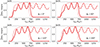 |
Fig. A.6. Same as in Fig. A.5 but for the NIR band (2.2 μm). |
| In the text | |
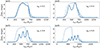 |
Fig. A.7. Same as in Fig. A.5 but for different initial azimuthal velocities. |
| In the text | |
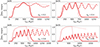 |
Fig. A.8. Same as in Fig. A.6 but for different initial azimuthal velocities. |
| In the text | |
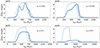 |
Fig. A.9. Same as in Fig. A.5 but for different radial blob velocities. |
| In the text | |
|
Fig. A.10. Same as in Fig. A.6 but for different radial blob velocities. |
| In the text | |
Current usage metrics show cumulative count of Article Views (full-text article views including HTML views, PDF and ePub downloads, according to the available data) and Abstracts Views on Vision4Press platform.
Data correspond to usage on the plateform after 2015. The current usage metrics is available 48-96 hours after online publication and is updated daily on week days.
Initial download of the metrics may take a while.