| Issue |
A&A
Volume 691, November 2024
|
|
|---|---|---|
| Article Number | A308 | |
| Number of page(s) | 25 | |
| Section | Catalogs and data | |
| DOI | https://doi.org/10.1051/0004-6361/202451761 | |
| Published online | 25 November 2024 | |
Value-added catalog of physical properties for more than 1.3 million galaxies from the DESI survey
1
Institute of Space Sciences, ICE-CSIC, Campus UAB, Carrer de Can Magrans s/n,
08913
Bellaterra, Barcelona,
Spain
2
Instituto Astrofisica de Canarias, Av. Via Lactea s/n,
38205
La Laguna,
Spain
3
Department of Physics and Astronomy, The University of Utah,
115 South 1400 East,
Salt Lake City,
UT
84112,
USA
4
Steward Observatory, University of Arizona,
933 N, Cherry Ave,
Tucson,
AZ
85721,
USA
5
Institut d’Estudis Espacials de Catalunya (IEEC), Edifici RDIT, Campus UPC,
08860
Castelldefels (Barcelona),
Spain
6
NSF NOIRLab,
950 N. Cherry Ave.,
Tucson,
AZ
85719,
USA
7
Lawrence Berkeley National Laboratory,
1 Cyclotron Road,
Berkeley,
CA
94720,
USA
8
Physics Dept., Boston University,
590 Commonwealth Avenue,
Boston,
MA
02215,
USA
9
Department of Physics & Astronomy, University College London,
Gower Street,
London
WC1E 6BT,
UK
10
Department of Physics & Astronomy, University College London,
Gower Street,
London
WC1E 6BT,
UK
11
Institute for Computational Cosmology, Department of Physics, Durham University,
South Road,
Durham
DH1 3LE,
UK
12
Instituto de Física, Universidad Nacional Autónoma de México, Cd. de México C.P.
04510
Mexico
13
Department of Physics & Astronomy and Pittsburgh Particle Physics, Astrophysics, and Cosmology Center (PITT PACC), University of Pittsburgh,
3941 O’Hara Street,
Pittsburgh,
PA
15260,
USA
14
Department of Physics & Astronomy, University College London,
Gower Street,
London
WC1E 6BT,
UK
15
Institut de Física d’Altes Energies (IFAE), The Barcelona Institute of Science and Technology, Campus UAB,
08193
Bellaterra Barcelona,
Spain
16
Departamento de Física, Universidad de los Andes,
Cra. 1 No. 18A-10, Edificio Ip,
CP
111711,
Bogotá,
Colombia
17
Observatorio Astronómico, Universidad de los Andes,
Cra. 1 No. 18A-10, Edificio H,
CP
111711
Bogotá,
Colombia
18
Institute of Cosmology and Gravitation, University of Portsmouth,
Dennis Sciama Building,
Portsmouth,
PO1 3FX,
UK
19
Fermi National Accelerator Laboratory,
PO Box 500,
Batavia,
IL
60510,
USA
20
Center for Cosmology and AstroParticle Physics, The Ohio State University,
191 West Woodruff Avenue,
Columbus,
OH
43210,
USA
21
Department of Physics, The Ohio State University,
191 West Woodruff Avenue,
Columbus,
OH
43210,
USA
22
The Ohio State University,
Columbus,
OH
43210,
USA
23
School of Mathematics and Physics, University of Queensland,
Queensland
4072,
Australia
24
Department of Physics, The University of Texas at Dallas,
Richardson,
TX
75080,
USA
25
Department of Physics, Southern Methodist University,
3215 Daniel Avenue,
Dallas,
TX
75275,
USA
26
Department of Physics and Astronomy, University of California,
Irvine
92697,
USA
27
Sorbonne Université, CNRS/IN2P3, Laboratoire de Physique Nucléaire et de Hautes Energies (LPNHE),
75005
Paris,
France
28
Departament de Física, Serra Húnter, Universitat Autònoma de Barcelona,
08193
Bellaterra (Barcelona),
Spain
29
Department of Astronomy, The Ohio State University,
4055 McPherson Laboratory, 140 W 18th Avenue,
Columbus,
OH
43210,
USA
30
Institució Catalana de Recerca i Estudis Avançats,
Passeig de Lluís Companys, 23,
08010
Barcelona,
Spain
31
Department of Physics and Astronomy, Siena College,
515 Loudon Road,
Loudonville,
NY
12211,
USA
32
Departamento de Física, Universidad de Guanajuato – DCI, C.P.
37150,
Leon, Guanajuato,
Mexico
33
Instituto Avanzado de Cosmología A. C.,
San Marcos 11 – Atenas 202. Magdalena Contreras,
10720.
Ciudad de México,
Mexico
34
Kavli Institute for Astronomy and Astrophysics at Peking University, PKU,
5 Yiheyuan Road, Haidian District,
Beijing
100871,
P.R.
China
35
Department of Physics and Astronomy, University of Waterloo,
200 University Ave W,
Waterloo,
ON
N2L 3G1,
Canada
36
Perimeter Institute for Theoretical Physics,
31 Caroline St. North,
Waterloo,
ON
N2L 2Y5,
Canada
37
Waterloo Centre for Astrophysics, University of Waterloo,
200 University Ave W,
Waterloo,
ON
N2L 3G1,
Canada
38
Space Sciences Laboratory, University of California,
Berkeley, 7 Gauss Way,
Berkeley,
CA
94720,
USA
39
University of California, Berkeley,
110 Sproul Hall #5800
Berkeley,
CA
94720,
USA
40
Instituto de Astrofísica de Andalucía (CSIC), Glorieta de la Astronomía, s/n,
18008
Granada,
Spain
41
Department of Physics and Astronomy, Sejong University,
Seoul,
143-747,
Korea
42
CIEMAT,
Avenida Complutense 40,
28040
Madrid,
Spain
43
Department of Physics, University of Michigan,
Ann Arbor,
MI
48109,
USA
44
University of Michigan,
Ann Arbor,
MI
48109,
USA
45
Department of Physics & Astronomy, Ohio University,
Athens,
OH
45701
USA
46
National Astronomical Observatories, Chinese Academy of Sciences,
A20 Datun Rd., Chaoyang District,
Beijing
100012,
P.R.
China
★ Corresponding author; This email address is being protected from spambots. You need JavaScript enabled to view it.
Received:
1
August
2024
Accepted:
1
October
2024
Abstract
Aims. We present an extensive catalog of the physical properties of more than a million galaxies investigated with the Dark Energy Spectroscopic Instrument (DESI), one of the largest spectroscopic surveys to date. Spanning a full range of target types, including emission-line galaxies, luminous red galaxies, and quasars, our survey encompasses an unprecedented range of spectroscopic redshifts, all the way from 0 to 6.
Methods. The physical properties, such as stellar masses and star formation rates, were derived via the CIGALE spectral energy distribution (SED) fitting code accounting for the contribution coming from active galactic nuclei (AGNs). Based on the modeling of the optical-mid-infrared (grz supplemented with WISE photometry) SEDs, we studied the galaxy properties with respect to their location on the main sequence.
Results. We have revised the dependence of stellar mass estimates on model choices and on the availability of WISE photometry. Indeed, the WISE data are required to minimize the misclassification of star-forming galaxies as AGNs. The lack of WISE bands in SED fits leads to elevated AGN fractions for 68% of star-forming galaxies identified using emission line diagnostic diagrams, but this does not significantly affect their stellar mass or star formation estimates.
Key words: catalogs / galaxies: active / galaxies: evolution / galaxies: general / galaxies: nuclei / galaxies: Seyfert
© The Authors 2024
 Open Access article, published by EDP Sciences, under the terms of the Creative Commons Attribution License (https://creativecommons.org/licenses/by/4.0), which permits unrestricted use, distribution, and reproduction in any medium, provided the original work is properly cited.
This article is published in open access under the Subscribe to Open model. This email address is being protected from spambots. You need JavaScript enabled to view it. to support open access publication.
1 Introduction
The exploration of galaxies has been a focal point of astronomical research for centuries, revealing an astonishing diversity of galaxy types and physical processes. Large galaxy photometric catalogs mapping an unprecedented number of galaxies and their properties, such as COSMOS (Scoville et al. 2007; Weaver et al. 2022), CANDELS (Grogin et al. 2011; Koekemoer et al. 2011), UltraVISTA (McCracken et al. 2012; Muzzin et al. 2013), and ZFOURGE (Straatman et al. 2016) supplemented with spectroscopic datasets, such as those of Sloan Digital Sky Survey (SDSS; York et al. 2000), Galaxy and Mass Assembly (GAMA; Baldry et al. 2018), Deep Extragalactic VIsible Legacy Survey (DEVILS; Davies et al. 2021), and VIMOS Public Extragalactic Redshift Survey (VIPERS; Scodeggio et al. 2018) have allowed us to unlock fundamental galaxy scaling relations and have made significant contributions to our understanding of galaxies and physical processes regulating their formation and evolution.
Template-based techniques relying on the spectral energy distribution (SED; e.g., Conroy 2013 and references therein) fitting of galaxies are generally used to derive physical properties of galaxies from large-scale sky surveys. These methods heavily depend on the physical models of galaxy populations (e.g., Mitchell et al. 2013; Moustakas et al. 2013; Lower et al. 2020; Pacifici et al. 2023) and a statistical method of finding the best fits (e.g., Leja et al. 2018). The optimization of the parameter space and priors in constructing a model library is vital for finely tuning parameters related to stellar populations, dust content, and other key factors. This precision enables a more accurate characterization of galaxies. Building an extensive variety of models is crucial to encompass the full diversity of galaxy properties, but it introduces challenges such as degeneracies, where different parameter combinations yield similar predictions (e.g., Lower et al. 2020). An excessively large model library also poses the risk of overfitting, whereby models may fit noise or peculiarities in the data, rather than capturing the genuine underlying physical properties of galaxies. The SED fitting demands a wide wavelength coverage for better tracing the contribution from all stellar types in a galaxy (e.g., Maraston et al. 2006; Pforr et al. 2019) and to break degeneracies between the host galaxy and the parameters related to the active galactic nucleus (AGN) (e.g., Calistro Rivera et al. 2016; Thorne et al. 2022a). Accounting for the AGN contribution is one of the most significant sources of uncertainty in estimated physical properties as AGNs are relatively common and their contribution to the mid-infrared (MIR) emission might be significant (Leja et al. 2018). The inferred physical properties also hinge on the accuracy of photometry and redshift of galaxies (e.g., Acquaviva et al. 2015; Iyer & Gawiser 2017; Paulino-Afonso et al. 2022). Thus, a careful consideration of the extensive range of possible model combinations within the parameter space is essential for the robust estimations of physical properties of galaxies (e.g., Pforr et al. 2012; Johnson et al. 2021; Han et al. 2023; Pacifici et al. 2023).
To address the aftermentioned challenges, a collection of panchromatic SED codes has been developed relying on the reduced ![Mathematical equation: $\[\chi^{2}\left(\chi_{\mathrm{r}}^{2}\right)\]$](/articles/aa/full_html/2024/11/aa51761-24/aa51761-24-eq1.png) techniques such as MAGPHYS (da Cunha et al. 2008), BEAGLE (Chevallard & Charlot 2016), Prospector (Johnson et al. 2021), BAGPIPES (Carnall et al. 2018), CIGALE (Boquien et al. 2019), and ProSpect (Robotham et al. 2020), along with the most recent SED fitting codes based on the Markov chain Monte Carlo (MCMC) approach, such as MCSED (Bowman et al. 2020), piXedfit (Abdurro’uf et al. 2021), Lightning (Doore et al. 2023), PROVABGS (Hahn et al. 2023a), and GalaPy (Ronconi et al. 2024), among others. Employing diverse forward-modeling frameworks or templates, along with a range of Bayesian methods such as MCMC sampling or on a model grid, these codes provide a comprehensive approach to accurately estimate the physical properties of galaxies. We refer to Pacifici et al. (2023) and Best et al. (2023) for a review of the performance of different SED fitting tools.
techniques such as MAGPHYS (da Cunha et al. 2008), BEAGLE (Chevallard & Charlot 2016), Prospector (Johnson et al. 2021), BAGPIPES (Carnall et al. 2018), CIGALE (Boquien et al. 2019), and ProSpect (Robotham et al. 2020), along with the most recent SED fitting codes based on the Markov chain Monte Carlo (MCMC) approach, such as MCSED (Bowman et al. 2020), piXedfit (Abdurro’uf et al. 2021), Lightning (Doore et al. 2023), PROVABGS (Hahn et al. 2023a), and GalaPy (Ronconi et al. 2024), among others. Employing diverse forward-modeling frameworks or templates, along with a range of Bayesian methods such as MCMC sampling or on a model grid, these codes provide a comprehensive approach to accurately estimate the physical properties of galaxies. We refer to Pacifici et al. (2023) and Best et al. (2023) for a review of the performance of different SED fitting tools.
The evolving landscape of astronomy and the state-of-the-art instruments, including Dark Energy Spectroscopic Instrument (DESI; DESI Collaboration 2016a, 2022), Prime Focus Spectrograph (PFS; Takada et al. 2014), Vera C. Rubin Observatory (Ivezić et al. 2019), James Webb Space Telescope (Gardner et al. 2006), Euclid (Laureijs et al. 2010), and Nancy Grace Roman Space Telescope (Spergel et al. 2015), demands an even deeper understanding of the physical properties of galaxies. We must also account for various target types, spanning a wider redshift range. In particular, the advent of large multi-wavelength surveys triggered using SED fitting methodology to constrain the AGN and its host galaxy properties for statistical samples (e.g., Walcher et al. 2011; Boquien et al. 2019; Johnson et al. 2021; Yang et al. 2020, 2022; Thorne et al. 2022b; Bichang’a et al. 2024). The importance of incorporating AGN templates for reliable estimates of physical properties of galaxies hosting AGNs was already raised in previous works, such as Ciesla et al. (2015). The SED fitting approach has revealed the potential to not only derive reliable properties of AGN and host properties (e.g., Marshall et al. 2022; Mountrichas et al. 2021a; Burke et al. 2022; Best et al. 2023) but also to identify AGNs based on their multi-wavelength information (e.g., Thorne et al. 2022b; Best et al. 2023; Yang et al. 2023; Prathap et al. 2024). The AGN SED modeling techniques are also used as the base for the target selection of forthcoming wide-field spectroscopic surveys such as 4MOST (Merloni et al. 2019) and VLT-MOONS (Maiolino et al. 2020).
In this paper, we describe the methodology employed in constructing the Value Added Catalog (VAC) of physical properties of DESI Early Data Release (EDR) galaxies obtained via SED modeling with the Code Investigating GALaxy Emission (CIGALE; Boquien et al. 2019). This code, based on the energy balance principle, has already proved its efficiency and accuracy in estimating physical properties accounting for the AGN contribution (e.g., Ciesla et al. 2015; Yang et al. 2023). Its modular framework allows the inclusion of various AGN models, both based on both theoretical approaches (e.g., Fritz et al. 2006) and observational constraints (e.g., Stalevski et al. 2012, 2016). We demonstrate the utility of our catalog by showcasing its potential for discriminating host galaxy properties, while also investigating the influence of the model assumptions and availability of photometry data. In the follow-up paper (Siudek et al. under DESI Collaboration review), we discuss the ability of the SED fitting approach to distinguish narrowline (NL) and broadline (BL) AGNs based on their physical properties. The structure of the paper is as follows. In Sect. 2, we provide an overview of the DESI survey and EDR data. In Sect. 3, we describe the SED fitting methodology applied to derive the physical properties of DESI galaxies. The general properties of the catalog are presented in Sect. 4. We compared our sample to existing catalogs to validate the derived properties of galaxies in Sect. 5. In Sect. 6, we discuss the dependence of the physical properties on model assumptions and MIR availability. Finally, Sect. 7 summarizes the catalog and our analysis. Throughout this paper, we assume WMAP7 cosmology (Komatsu et al. 2011), with Ωm = 0.272 and H0 = 70.4. We also consider the photometry in AB magnitudes (Oke & Gunn 1983).
2 DESI data
2.1 DESI survey
DESI is a 5000-fiber multiobject spectrograph installed on the Mayall 4-meter telescope at Kitt Peak National Observatory. It covers a spectral range of 3600–9800 Å with a wavelength-dependent spectral resolution, R = 2000–5500 (DESI Collaboration 2016b; DESI Collaboration 2022; Miller et al. 2024; Silber et al. 2023). It is designed to observe approximately 36 million galaxies (Hahn et al. 2023b; Raichoor et al. 2023; Zhou et al. 2023) and 3 million quasars (Chaussidon et al. 2023) over a 14000 deg2 within a five-year period (DESI Collaboration 2024a) with the aim to determine the nature of dark energy through the most precise measurement of the expansion history of the universe ever obtained (Levi et al. 2013). The DESI dataset will be ten times larger than the SDSS (York et al. 2000; Almeida et al. 2023) sample of extragalactic targets and substantially deeper than prior large-area surveys (DESI Collaboration 2024a). In December 2020, DESI started a fivemonth survey validation (SV) before the start of the main survey (DESI Collaboration 2024b). The SV campaign consisted of three phases: i) SV1: validating the target selections of the five primary target classes: Milky Way survey (MWS; Cooper et al. 2023) and bright galaxy survey (BGS; Hahn et al. 2023b), along with surveys of luminous red galaxies (LRG; Zhou et al. 2023), emission-line galaxies (ELG; Raichoor et al. 2023), and quasars (QSO; Chaussidon et al. 2023). These targets were further supplemented with secondary fiber targets for additional science goals (SCND; e.g., Darragh-Ford et al. 2023; Fawcett et al. 2023. More details regarding the DESI targeting are described in Myers et al. 2023); Furthermore, ii) SV2: operation developments; and iii) SV3 (One-Percent survey) optimized the observing procedures (Schlafly et al. 2023), with very high fiber assignments completeness over an area of 200 deg2, namely, of 1% of the final DESI main survey. The entire SV data, internally known as Fuji, is publicly released as the DESI Early Data Release (EDR; DESI Collaboration 2024a) and is used for generating the VAC of physical properties of DESI galaxies presented in this paper. The First Data Release (DR1, DESI Collaboration et al. in prep.) is planned to be released at the first half of 2025. The DR1 already showcases the DESI potential in science Key Papers presenting the two-point clustering measurements and validation (DESI Collaboration et al. in prep.), BAO measurements from galaxies and quasars (DESI Collaboration 2024e), and from the Lya forest (DESI Collaboration 2024d), as well as a full-shape studies of galaxies and quasars (DESI Collaboration et al. in prep). These are supplemented with the cosmological results from the BAO measurements (DESI Collaboration 2024c) and the full-shape analysis (DESI Collaboration et al., in prep.), as well as constraints on primordial non-gaussianities (DESI Collaboration et al., in prep.).
The DESI spectra are processed with a fully automatic pipeline (Guy et al. 2023), followed by the spectral classification and redshift estimation using the Redrock pipeline1 (Anand et al. 2024, Bailey et al. in prep.). This χ2 method relies on the principal component analysis templates generated from a combination of real and synthetic spectra of astronomical sources using an iterative principal component generator (Bailey 2012), which also takes the uncertainties of the data into account. Along with the redshift (Z), we take the redshift uncertainty (ZERR), a redshift warning bitmask (ZWARN), Redrock also assigns a spectral type (SPECTYPE) to every target based on the best fit. The resulting DESI EDR redshift catalog consists of 2 847 435 spectra of 2 757 937 unique sources (DESI Collaboration 2024a). For multiply observed targets, we chose the “best” spectrum as the one that has a higher signal-to-noise ratio (S/N) spectrum, along with good fiber and redshift measurements (ZCAT_PRIMARY = True2). Furthermore, we selected sources that have been assigned as GALAXY or QSO by Redrock and that do not have any fiber issues (COADD_FIBERSTATUS = 03), but do have a reliable redshift (ZWARN = 0 or 44). We refer to DESI Collaboration 2024a for more details about our selection choices. After applying all these cuts, we were left with a sample of 1345137 objects spanning a redshift range of 0.001 ≤ z ≤ 5.968 over ~1100 deg2. Our analysis requires photometric measurements, which are described in the following subsection.
2.2 Photometry
The DESI primary targets (MWS, BGS, LRG, ELG, and QSO) were selected from the ninth data release of the Legacy imaging surveys5 (LS/DR9; Dey et al. 2019), which is a combination of three public projects. The northern sky is covered by the BeijingArizona Sky Survey (BASS; Zou et al. 2017) in the g and r band and by the Mayall z-band Legacy Survey (MzLS) in the z band with a 5σ detection limit of g = 23.48, r = 22.87, and z = 22.29 AB magnitude. The south LS footprint is mapped by the Dark Energy Camera Legacy Survey (DECaLS) in all three bands (g, r, and z) with a 5σ detection of g = 23.72, r = 23.27, and z = 22.22 AB magnitude. The detection limits are found for a fiducial galaxy size of 0.45″.
The ground-based optical and near-infrared (NIR) photometry (i.e., grz photometry, which we hereafter shortly refer to as optical) is supplemented with observations from MIR bands at 3.4, 4. 6, 12 and 22 μm provided by the Wide-field Infrared Survey Explorer (WISE; Wright et al. 2010) and a mission extension NEOWISE-Reactivation forced-photometry (Mainzer et al. 2014) in the unWISE maps at the DESI footprint (Meisner et al. 2017; Schlafly et al. 2019; Meisner et al. 2021a). The WISE photometry is matched to optical imaging using the Tractor package (Lang et al. 2016) based on seven-year custom stacks of WISE/NEOWISE exposures, called unWISE coadds, reaching 5σ limiting magnitudes of 21.7 and 20.9 AB mag in W1 and W2 (Meisner et al. 2019, 2021b). Table 1 summarizes the information about photometric bands used in this analysis.
Tractor is a pioneered Python tool based on the statistically rigorous forward-modeling approach to perform source extraction on the pixel data. It is designed to fit images and photometry to estimate source shapes and brightness properties taking into account their different point spread function (PSF) and different band sensitivities. This approach is particularly useful to process LS sources given their wide range of PSF shapes and sizes: the optical data have a typical PSF of ~1 arcsec; and the WISE PSF full width at half maximum (FWHM) is ~6 arcsec in Wl–W3 and ~12 arcsec in W4 (Dey et al. 2019). The pixels associated with each detection (called blob) are fitted with models of surface brightness, including the Sérsic profile, and the best fit is chosen as the one which minimizes the ![Mathematical equation: $\[\chi_{\mathrm{r}}^{2}\]$](/articles/aa/full_html/2024/11/aa51761-24/aa51761-24-eq2.png) . The fits are performed separately on each photometric band (g, r, and z bands) accounting for different PSF and sensitivity of each image. In DR9, the light profiles are fitted with four models: point source (PSF), round exponential galaxy model (REX), de Vaucouleurs model (DEV), exponential model (EXP), and a Sérsic model (SER)6, in that order. However, Tractor models do not include more complex structures and the resulting models may not always be ideal. The best-fit model is determined by convolving each model with the specific PSF for each exposure, fitting it to each image, and minimizing the residuals for all images.
. The fits are performed separately on each photometric band (g, r, and z bands) accounting for different PSF and sensitivity of each image. In DR9, the light profiles are fitted with four models: point source (PSF), round exponential galaxy model (REX), de Vaucouleurs model (DEV), exponential model (EXP), and a Sérsic model (SER)6, in that order. However, Tractor models do not include more complex structures and the resulting models may not always be ideal. The best-fit model is determined by convolving each model with the specific PSF for each exposure, fitting it to each image, and minimizing the residuals for all images.
The Tractor model fits are determined using only the optical (grz) data. The MIR photometry for each optically detected source is then determined by forcing the location and shape of the model, convolving with the WISE PSF, and fitting to the WISE stacked image. The advantage of the “forced photometry” is the ability to deblend any confused WISE sources by using the higher-spatial-resolution optical data and detecting fainter sources than traditional approaches, while preserving the photometric reliability. However, this approach limits the LS catalog to strictly WISE photometry for sources detected at optical wavelengths (Dey et al. 2019).
Tractor returns the object position, fluxes, galactic extinctions, shape, and morphological parameters, given by the Sérsic index (among others). The Tractor catalog also contains a set of quality measures, such as FRACMASKED, FRACFLUX, and FRACIN, which offer a qualitative calculation of the data in each profile fit and can be used to preselect high-quality samples (see Sect. 4.1). More detail about the data reduction can be found in Dey et al. (2019) and Schlegel et al., in prep.
In addition to the primary targets, DESI EDR also includes some secondary targets and targets of opportunity that do not have LS/DR9 photometry. Given that our analysis requires photometric measurements, we only consider the DESI sources that have LS/DR9 photometry (RELEASE = 9010 or 9011 or 9012). This leads to a final sample of 1286124 unique objects, spanning a redshift range of 0.001 ≤ z ≤ 5.968. The demographics of the DESI primary targets (MWS, BGS, LRG, ELG, and QSO) is summarized in Table 2. The redshift distribution of all these sources, along with their distributions from different targeting types is shown in Fig. 1, with the distribution of MWS scaled up by a factor of ten to more easily compare the shape of each distribution. The DESI VAC covers a wide redshift range spanning over z = 0–6 targeting BGS galaxies and AGNs at lower redshift (z < 0.6; Hahn et al. 2023b; Juneau et al. 2024) and ELGs at higher redshift (0.6 < z < 1.6; Raichoor et al. 2023), with QSOs spanning out to z ~ 6 (Chaussidon et al. 2023); LRGs extend out to z ~ 1 (Zhou et al. 2023) and SCND sources cover the entire redshift range, incorporating low-z targets (e.g., Darragh-Ford et al. 2023) as well as high-z QSOs (e.g., Fawcett et al. 2023). The catalog also includes a negligible fraction (< 1%) of galaxies and QSO observed within the MWS (Cooper et al. 2023) spanning a wide redshift range; namely, it is composed of 3238 galaxies (with a mean redshift z = 0.7) and 6052 QSOs (with a mean redshift z = 1.6).
Summary of the LS9 photometry used for SED fitting.
Summary of DESI main target classes used throughout the paper.
3 Spectral energy distribution fitting
Physical properties of DESI galaxies are derived by performing SED (optical and mid-IR photometry) fitting using Code Investigating GALaxy Emission (CIGALE v2022.1; Boquien et al. 2019). CIGALE is a state-of-the-art Python code based on the principles of the energy balance between the dust-absorbed stellar emission in the ultraviolet (UV) and optical and its re-emission in the infrared (IR). Thanks to its efficiency, flexibility, and accuracy, CIGALE and its modified version X-CIGALE (Yang et al. 2020, 2022) are widely used to derive the physical properties of galaxies and AGNs in large galaxy surveys (e.g., Ciesla et al. 2015; Salim et al. 2016, 2018; Małek et al. 2018; Barrows et al. 2021; Mountrichas et al. 2021b; Zou et al. 2022; Csizi et al. 2024; Osborne & Salim 2024) as well as high-z AGNs (e.g., Conselice et al. 2023; Mezcua et al. 2023; Yang et al. 2023; Burke et al. 2024; Durodola et al. 2024). CIGALE estimates the physical properties of galaxies using a Bayesian approach by evaluating all the possible combinations of SED models on data to maximize the likelihood distribution. CIGALE takes into account the age of the universe at the redshift of each object when fitting models. It excludes stellar population ages that exceed the age of the universe at the given redshift. This constraint helps us avoid unphysical solutions and ensures the consistency of the fitted parameters with cosmological constraints. The estimates and errors of the physical properties are then computed as the likelihood-weighted mean and standard deviation, respectively, for all the models (Boquien et al. 2019). To build a library of models, CIGALE relies on five main modules: star formation history (SFH), SSP models, dust attenuation and emission, and the AGN component. For each module, CIGALE includes several possible prescriptions and the flexible parametrization of model parameters allows us to adapt the model complexity (i.e., number of free parameters). In the next sections, we describe the key assumptions and parametrization of models used to create our catalog, which are summarized in Table 3. This configuration generates 167 529 600 models spanning over a wide redshift range from 0 to 6 (302 400 per redshift). We use a single node of 32 cores on the Cori supercomputer at the National Energy Research Scientific Computing Center (NERSC) to fit all SEDs within 3.5 hours.
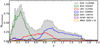 |
Fig. 1 Redshift distribution of the DESI EDR sources with reliable redshift and photometry estimates (see Sect. 2). The catalog includes all galaxies and quasars observed within the DESI target classes: BGS, LRG, ELG, QSO, SCND, and MWS. The redshift distribution of MWS targets is scaled up by a factor of 10. Some of the sources are targeted by multiple target classes. The numbers shown in the figure also contain duplicates, so this total is higher than the number of unique targets. |
3.1 Stellar component
We use the Bruzual & Charlot (2003) SSP models adopting a Chabrier (2003) IMF to build the stellar component. We assume solar metallicity and following the analysis by Ciesla et al. (2015), we use the delayed SFH with an optional exponential burst. This prescription allows us to reproduce the SEDs of both star-forming and passive galaxies with a modest number of free parameters (e.g., Ciesla et al. 2015; Salim et al. 2016). Such two exponentially decreasing star formation rate (SFR) laws with different e-folding times show a good performance in decoupling the long-term SFH from the recent star formation activity (Ciesla et al. 2015; Małek et al. 2018). The SFR is therefore defined as the sum of two exponentially decreasing SFRs:
![Mathematical equation: $\[\operatorname{SFR}(\mathrm{t})=\operatorname{SFR}_{\text {delayed}}(\mathrm{t})+\mathrm{SFR}_{\text {burst}}(\mathrm{t}),\]$](/articles/aa/full_html/2024/11/aa51761-24/aa51761-24-eq3.png) (1)
(1)
where:
![Mathematical equation: $\[\mathrm{SFR}_{\text {delayed}}(\mathrm{t}) \propto \mathrm{te}^{-\mathrm{t} / \tau_{\text {main}}},\]$](/articles/aa/full_html/2024/11/aa51761-24/aa51761-24-eq4.png) (2)
(2)
and
![Mathematical equation: $\[\operatorname{SFR}(\mathrm{t})_{\text {burst }}= \begin{cases}\mathrm{e}^{-\mathrm{t} / \tau_{\text {min }}}, & \text { if } \mathrm{t}<\mathrm{t}_{\text {main }}-\mathrm{t}_{\text {burst}}, \\ \mathrm{e}^{-\mathrm{t} / \tau_{\text {min }}}+\mathrm{k} \times \mathrm{e}^{-\mathrm{t} / \tau_{\text {burst }}} & \text { if } \mathrm{t} \geq \mathrm{t}_{\text {main }}-\mathrm{t}_{\text {burst}},\end{cases}\]$](/articles/aa/full_html/2024/11/aa51761-24/aa51761-24-eq5.png) (3)
(3)
where t is the time, τmain is the e-folding time of the main (old) stellar population, τburst is the e-folding time of the burst (young) stellar population, and k is the amplitude of the second exponential which depends on the fraction of stars formed in the second burst versus the total stellar mass formed (fySP). The SFH module is described in more detail in Ciesla et al. (2015, 2017).
The effects of the choice of IMF, the SFH prescription, and the solar metallicity assumption on the main galaxy physical properties are discussed in Sect. 6.
Default parameters used in SED fitting with CIGALE.
3.2 Nebular emission
Nebular emission (emission from ionized gas) is an important component to include when considering high-redshift galaxies (e.g., Stark et al. 2013; de Barros et al. 2014; Yuan et al. 2019) or at lower-redshift starburst dwarf and young star-forming galaxies (e.g., Boquien et al. 2010) as intense star formation and ionization processes lead to stronger nebular emission signatures. Neglecting the nebular emission component may lead to the overestimation of the stellar mass (Yuan et al. 2019). The nebular emission lines are pre-computed with CLOUDY 17.01 (Ferland et al. 2017) with electron density (Ne), gas metallicity (Zgas), and ionization parameter (U) as the free parameters and re-scaled with the number of Lyman continuum photons from the stellar emission. The Bruzual & Charlot (2003) SSP models using a constant SFH over 10 Myr is used to generate the photoionizing field shape. The nebular continuum is scaled directly from the number of ionizing photons. CIGALE takes into account also the fraction of the Lyman photons escaping galaxies and absorbed by dust. More details about the implementation of the CLOUDY into CIGALE can be found in Villa-Vélez et al. (2021). We retained the default parameters of this module (see Table 3).
3.3 Interstellar dust
Dust is a fundamental component of galaxies that significantly influences their observed SEDs, especially those that are actively star-forming (Conroy 2013). It plays a dual role in stellar population models, as dust absorbs short-wavelength light (from the UV to NIR) and re-emits it at longer wavelengths (from MIR to far-infrared (FIR)). SED fitting techniques, such as those employed by CIGALE, model the full SED by simultaneously considering both the attenuated light and the re-emitted radiation. This integrated approach ensures that both the absorption and emission by dust are used to constrain the model. This is important because dust obscuration is influenced by the galaxy’s geometry, while dust emission is sensitive to the interstellar radiation field (Conroy 2013). Dust emission is dominated by: i) polycyclic aromatic hydrocarbon (PAH) bands in the MIR (~8 μm), ii) very small, warm grains, and iii) big, relatively cold grains (≳100 μm). Differences between these dust grains have an impact on the dust SED. On the other hand, attenuation also depends on the geometry. The simplest way to model dust attenuation is to assume attenuation laws (Boquien et al. 2019). CIGALE provides two modules to model attenuation curves: the implementation of the Charlot & Fall (2000) model and the modified Calzetti et al. (2000) model; for simplicity, we refer to it as the Calzetti et al. (2000) model.
The starburst model uses the Calzetti et al. (2000) starburst attenuation curve as a baseline, which is extended by a Leitherer et al. (2002) curve from the Lyman break to 150 nm. The amount of attenuation is described by the color excess applied to the nebular emission lines, E(B − V)line, and the ratio E(B − V)star/E(B − V)line, where E(B − V)star is the color excess applied to the whole stellar continuum. Following the Calzetti et al. (2000) recommendations, this ratio is fixed to 0.44. We used the Calzetti et al. (2000) model to generate our catalog; however, the impact on the physical property estimates when using Charlot & Fall (2000) is discussed in Sect. 6.2.
CIGALE provides five modules to describe the IR emission from dust: Casey (2012), Dale et al. (2014), Draine & Li (2007) and its updated version of the Draine et al. (2014) model, along with the Themis dust emission models from Jones et al. (2017). To create our catalog, we rely on the Draine et al. (2014) models, which account for very different physical conditions with a variety of radiation fields and a variable PAH emission providing a high flexibility. The model assumes that the majority (1 − γ) of dust mass is heated by a radiation field with an intensity (Umin), while the remaining fraction (γ) is exposed to intensities ranging from Umin to Umax following a power-law index α. By default, γ and α are fixed values set to 0.02, and 2, respectively. We also considered the model from Dale et al. (2014) and describe its influence on the physical properties of galaxies in Sect. 6.2.
3.4 AGN contribution
CIGALE allows for the separation of the emission from AGN from their host galaxy with several approaches, starting from a simple AGN parameterization by the power slope when using Casey (2012) models to fit IR data. The Dale et al. (2014) module provides simple templates of quasars from UV to IR, with the AGN fraction left as a free parameter. Those options are fast but do not provide complex AGN SEDs. However, CIGALE also incorporates two more flexible models: Fritz et al. (2006) and SKIRTOR (Stalevski et al. 2012, 2016). The AGN model from Fritz et al. (2006) covers the UV to IR and assumes that the central engine is surrounded by smoothly distributed dust in the AGN torus (i.e., the AGN unified model; e.g., Zou et al. 2019), while SKIRTOR models add the possibility that the dust is clumpy (e.g., Stalevski et al. 2012; Assef et al. 2013). However, it is still unclear whether observations can discriminate between these models (Feltre et al. 2012).
In this work, we apply the Fritz et al. (2006) model, which uses a simple, but realistic torus geometry that relies on the flared disc and a full range of dust grain size. It allows us to control the geometry and physics of the torus thanks to a flexible ratio of the maximum to minimum radii of the dust torus, the optical depth at 9.7 μm, dust density distribution, opening angle of the torus, and the viewing angle. In particular, viewing from the equatorial direction (with a viewing angle AGNPSY = 0°) leads to the obscuration of the central engine and only the radiation reemitted in IR can be observed (type 2 AGN, i.e., NL AGN). When viewing from the polar direction (with a viewing angle AGNPSY = 90°), the central engine is directly visible (type 1 AGN, i.e., BL AGN). We fixed the parameters to the default, aside from allowing for the flexibility in the viewing angle (AGNPSY) and in the AGN fraction (AGNFRAC), defined as the ratio of the AGN IR emission to the total IR emission. Thus, the generated models cover a wide range of objects, including galaxies without any AGN contribution, as well as type 1 and 2 AGNs. This provides flexibility and allows us to build the catalog of physical properties for both AGN and non-AGN host galaxies. The impact of the incorporation or the change of the AGN model is discussed in Sect. 6.3.
4 VAC: General properties
In this section, we characterize the VAC of physical properties of the DESI galaxies and quasars observed at redshift 0.001 ≤ z ≤ 5.968 (see Sect. 2 for data description). The catalog includes all DESI sources, independent of their target class (BGS, LRG, ELG, SCND, MWS, and QSO) or redshift. The physical properties are derived based on the SED fitting using CIGALE (see Sect. 3 for the description of the SED procedures and modules and Table 3 for a full list of parameters). The catalog includes estimates of stellar masses, SFRs, absolute magnitudes, AGN fractions, and AGN luminosities among others (for the full list, see Table A.1).
4.1 Selection of galaxies: SEDs with secure fits
The DESI VAC includes all ‘reliable’ sources from the EDR (see Sect. 2 for the cuts applied for sample selection). The choice of additional cleaning cuts strongly depends on individual scientific goals. For general analysis of DESI galaxies, we did not introduce strict cuts to clean the sample, but the cuts can be adjusted as required for the specific science case. In the following analysis, we have excluded:
153 294 (12%) sources for which log(Mstar/M⊙) = 0. Almost all sources with log(Mstar/M⊙) = 0 are characterized by insufficient photometric observations to perform a reliable SED fitting. In particular, half of them are observed in only one optical band with a high signal to noise ratio (S/N ≥ 10); 21% of them have two or three optical observations with S/N ≥ 10, and only 3% are observed in two or more WISE bands with S/N ≥ 3. This suggests that these sources are false detections, faint sources, and other artifacts without valid photometry.
An additional 3231 (0.2%) sources with bad fits characterized by
![Mathematical equation: $\[\chi_{\mathrm{r}}^{2}\]$](/articles/aa/full_html/2024/11/aa51761-24/aa51761-24-eq6.png) > 17 (see Appendix D.2 for the description of the
> 17 (see Appendix D.2 for the description of the ![Mathematical equation: $\[\chi_{\mathrm{r}}^{2}\]$](/articles/aa/full_html/2024/11/aa51761-24/aa51761-24-eq7.png) cut). We note that the user may apply a more restrictive cut on
cut). We note that the user may apply a more restrictive cut on ![Mathematical equation: $\[\chi_{\mathrm{r}}^{2}\]$](/articles/aa/full_html/2024/11/aa51761-24/aa51761-24-eq8.png) (e.g.,
(e.g., ![Mathematical equation: $\[\chi_{\mathrm{r}}^{2}\]$](/articles/aa/full_html/2024/11/aa51761-24/aa51761-24-eq9.png) = 5) or apply further statistical criteria, such as a Bayesian information criterion (BIC; see e.g., Masoura et al. 2018; Buat et al. 2021). Figure 2 shows the distribution of
= 5) or apply further statistical criteria, such as a Bayesian information criterion (BIC; see e.g., Masoura et al. 2018; Buat et al. 2021). Figure 2 shows the distribution of ![Mathematical equation: $\[\chi_{\mathrm{r}}^{2}\]$](/articles/aa/full_html/2024/11/aa51761-24/aa51761-24-eq10.png) for DESI EDR galaxies.
for DESI EDR galaxies.
Additionally, the user can introduce several other quality cuts based on additional flags provided in the catalog, namely:
The S/N of the optical photometry. The uncertainties in stellar mass estimates strongly depend on the input photometry (see Appendix B for details). Sources observed in three optical bands (grz) with high S/N (S/N ≥ 10) are characterized by a stellar mass error of log(Mstar/M⊙)err ≲ 0.25, corresponding to the standard uncertainty of the stellar mass estimates due to model assumptions (see Sect. 6 and Conroy 20137, Pacifici et al. 2023). The FLAGOPTICAL defines the number of optical bands with S/N ≥ 10 and can be used to select sources with more reliable photometry and, thus, better estimates of the physical properties.
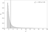
Fig. 2 Distribution of the
![Mathematical equation: $\[\chi_{\mathrm{r}}^{2}\]$](/articles/aa/full_html/2024/11/aa51761-24/aa51761-24-eq11.png) for the DESI EDR SED fits. The mean and standard deviation of
for the DESI EDR SED fits. The mean and standard deviation of ![Mathematical equation: $\[\chi_{\mathrm{r}}^{2}\]$](/articles/aa/full_html/2024/11/aa51761-24/aa51761-24-eq12.png) are reported in the legend. The dashed line corresponds to the mean
are reported in the legend. The dashed line corresponds to the mean ![Mathematical equation: $\[\chi_{\mathrm{r}}^{2}\]$](/articles/aa/full_html/2024/11/aa51761-24/aa51761-24-eq13.png) . At least ~ 88% of the sample is characterized by robust fits (defined as
. At least ~ 88% of the sample is characterized by robust fits (defined as ![Mathematical equation: $\[\chi_{\mathrm{r}}^{2}\]$](/articles/aa/full_html/2024/11/aa51761-24/aa51761-24-eq14.png) < 5):
< 5):The S/N of the WISE photometry. The availability of WISE photometry with high S/N (S/N ≥ 3) has an impact not only on the stellar mass estimates (see Sect. 6.4), but also on stellar mass errors (see App. B). The FLAGINFRARED defines the number of bands (WI–4) with S/N ≥ 38.
The probability density function (PDF) of the estimated parameters is asymmetric or multi-peaked. CIGALE introduces two estimates based on the best-fit model (best) and the likelihood-weighted mean measured from its PDF marginalized over other parameters (bayes). A narrow, one-peak PDF should see very similar values for these estimates; otherwise the PDF would end up asymmetric or multi-peaked. The shape of the PDF for the stellar mass and SFR estimates is expressed as FLAG_MASSPDF = logMbest/logMbayes and FLAG_SFRPDF = logSFRbest/logSFRbayes, respectively. To preselect sources with narrow one-peak PDF of stellar mass (SFR), we can consider only the one with values between 0.2 ≤ LOGMPDF(LOGSFRPDF) ≤ 5, following Mountrichas et al. (2021b), and Mountrichas et al. (2024).
Additional cuts based on the Tractor photometry information. To reject fragmented sources, we may introduce the cut: FRACFLUX ≤ 0.25 as advised by Juneau et al. (2024), Pucha et al. under DESI Collaboration review.
Our final EDR sample after cleaning features 1129599 sources (88% of the whole catalog) and is characterized by a mean ![Mathematical equation: $\[\overline{\chi_{\mathrm{r}}^{2}}=2.9 \pm 2.3\]$](/articles/aa/full_html/2024/11/aa51761-24/aa51761-24-eq15.png) (see Fig. 2). At least ~80% of the sample is characterized by good fits defined with a more strict criterion of
(see Fig. 2). At least ~80% of the sample is characterized by good fits defined with a more strict criterion of ![Mathematical equation: $\[\chi_{\mathrm{r}}^{2}\]$](/articles/aa/full_html/2024/11/aa51761-24/aa51761-24-eq16.png) ≲ 5 (Masoura et al. 2018; Buat et al. 2021).
≲ 5 (Masoura et al. 2018; Buat et al. 2021).
The distributions of SED-derived properties: rest-frame g-r color, stellar mass, and SFR of the DESI EDR galaxies are shown in Fig. 3. The distribution shapes are clearly different for each of the main target classes (MWS is scaled up by 10 to ease the comparison). The LRG are found among the reddest observed galaxies, while ELG are among the bluest with BGS bridging both the blue and red ends of the distribution (see the top panel in Fig. 3). QSO, MWS, and SCND are among the blue population. The stellar mass distribution follows the distribution of the g-r color, namely, the redder target class, LRG, is also found to be the one covering the high-mass end of the DESI EDR distribution (log(Mstar/M⊙) > 11), while the blue ELG peaks at log(Mstar/M⊙) ~ 9.5 − 10 forming a long tail towards the low-mass end. The remaining target classes (BGS, QSO, SCND, and MWS) are peaking in-between ELG and LRG covering log(Mstar/M⊙) ~ 10–11. As expected, LRG are characterized by lower SFR (log(SFR/M⊙yr−1) < 0) while ELG peak at higher SFR (log(SFR/M⊙yr−1) ~ 1), with MWS found to be among the most active (log(SFR/M⊙yr−1) > 2).
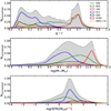 |
Fig. 3 Distribution of the SED-derived properties: rest-frame g-r color (top panel), stellar mass (log(Mstar/M⊙); middle panel), and star formation rate (SFR; bottom panel) of 1286124 of DESI EDR galaxies. The MWS target class is scaled up by a factor of ten. |
4.2 Star formation main sequence
One of the common indicators of the galaxy’s current star formation activity is its relation between SFR and stellar mass (Mstar − SFR), commonly known as the star-forming main sequence (MS). The position of a galaxy compared to the MS helps in classifying it as either a star-burst galaxy (above the MS), a passive galaxy (below the MS), or as a normal SF galaxy (close to the MS; e.g., Elbaz et al. 2007; Noeske et al. 2007; Whitaker et al. 2012; Johnston et al. 2015; Davies et al. 2016; Siudek et al. 2018; Davies et al. 2024). The MS relation exists across a range of epochs and environments and is roughly linear, with the normalization increasing with redshift (e.g., Schreiber et al. 2015; Lee et al. 2015; Thorne et al. 2021) suggesting that the majority of star-forming galaxies are in a self-regulated equilibrium state (e.g., Bouché et al. 2010; Daddi et al. 2010; Genzel et al. 2010; Lagos et al. 2011; Lilly et al. 2013; Davé et al. 2013; Mitchell et al. 2016).
In this paper, we demonstrate the MS relation for BGS galaxies. The BGS sample is a flux-limited survey at low redshift (0 < z < 0.6) divided into two programs: BRIGHT with r < 19.5 and DARK reaching fainter galaxies at 19.5 < r < 20.175 (Hahn et al. 2023b). We utilized the rest-frame colors derived with CIGALE: U − V vs. V − J to construct the UVJ diagram (Williams et al. 2009; Whitaker et al. 2012) used to identify red and blue galaxies. The UVJ diagram for a sample of 356 304 BGS (BRIGHT and DARK) galaxies9 is shown in Fig. 4 with a separation cut following the definition given by Whitaker et al. (2012): U − V > 0.8 × (V − J) + 0.7, U − V > 1.3 and V − J < 1.510. A gradual change in the specific SFR (sSFR) with colors is evident. Red galaxies are characterized by low sSFR (log(sSFR/y−1) ≲ 11), while blue galaxies are actively star forming (log(sSFR/y−1) ≳ 10).
The distribution of stellar mass and SFR for red and blue galaxies is shown in Fig. 5. We find a similar number of red and blue galaxies (48%, and 52%, respectively) among the fluxlimited BGS sample, with a mean stellar mass log(Mstar/M⊙) = 10.71 and 9.89 for red and blue galaxies, respectively (see left panel in Fig. 5). As expected, the massive red galaxies are characterized by lower SFRs than low-mass blue galaxies (with a mean SFR log(SFR) = −6.4 and 0.3 M⊙yr−1 for red and blue galaxies, respectively; see right panel in Fig. 5). The blue galaxies tend to follow the MS according to Schreiber et al. (2015) with slightly higher SFR values possibly due to the choice of the dust attenuation prescription (see e.g., Siudek et al. 2018). The clear MS trend not only validates the SED fitting procedures in recreating the proper physical properties for a population of BGS galaxies but also showcases the utility of derived restframe colors for galaxy classification purposes. We note that to quantitatively compare the fraction and properties of red and blue galaxies one should take into account the selection biases. For example, selecting a mass complete sample (selected following prescription from Pozzetti et al. 2010) changes the fraction of red and blue galaxies to 68% and 32%, respectively.
In Fig. 6, the MS trend of star-forming galaxies observed at a median redshift of the BGS sample (z ~ 0.24; the median redshift of the BGS sample) is reproduced following the prescription given by Schreiber et al. (2015). Starburst and passive galaxies are commonly selected as galaxies that deviate for more than +0.6 dex, and −0.6 dex from the MS, respectively (e.g., Elbaz et al. 2007; Rodighiero et al. 2011; Sargent et al. 2012; Whitaker et al. 2012; Buat et al. 2019; Donevski et al. 2020). The lower limits distinguishing passive galaxies correspond to the transition between red and blue galaxies selected based on the UVJ diagram. The bulk of blue BGS galaxies are located close to the MS, while the red BGS are found under the MS.
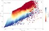 |
Fig. 4 UVJ diagram for BGS galaxies observed at redshift 0 < z < 0.6 color-coded according to their sSFR estimates. Red and blue galaxies are selected by the cut defined by Whitaker et al. (2012) shown in black. |
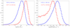 |
Fig. 5 Stellar mass (left) and SFR (right) distributions for red (in red) and blue (in blue) BGS galaxies observed at redshift 0 < z < 0.6 with means and standard deviations reported in the legend. Red and blue galaxies are selected by the cut defined by Whitaker et al. (2012) in the UVJ diagram (see Fig. 4). |
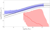 |
Fig. 6 Mstar – SFR relation for BGS galaxies. The MS at z ~ 0.24 (median redshift of the BGS sample) according to Schreiber et al. (2015) is shown with a black solid line, while dashed lines correspond to MS ± 0.6 dex to represent starburst and passive galaxies. The running median and 16th-84th percentile range for red and blue galaxies selected based on the UVJ criterion are marked with red and blue, respectively. |
5 Comparison to other catalogs
In this section, we compare our estimates of the physical properties of DESI EDR galaxies with the COSMOS (Weaver et al. 2022), AGN-COSMOS (Suh et al. 2019 and Thorne et al. 2022b), and DEVILS (Thorne et al. 2022b) catalogs. In Appendix C, we further compare our estimates with: i) SDSS and Extended Baryon Oscillation Spectroscopic Survey (eBOSS) Firefly VAC (SDSS(Firefly DR16); Comparat et al. 2017), ii) SDSS MPAJHU DR8, after the Max Planck Institute for Astrophysics and Johns Hopkins University (SDSS(MPA-JHU); Kauffmann et al. 2003b; Brinchmann et al. 2004; Tremonti et al. 2004), iii) GALEX-SDSS-WISE Legacy Catalog X211 (GSWLC; Salim et al. 2016, 2018), and iv) DESI VAC of the stellar masses and emission lines presented by Zou et al. (2024). The summary of the comparison of stellar masses from different catalogs (including the ones described in Appendix C for simplicity) is presented in Table 4, using metrics described in Sect. 5.1 to quantify the differences. There exist several other DESI VACs with stellar mass estimates, such as i) FastSpecFit Spectral Synthesis and Emission-Line Catalog FastSpecFit 3.2 (Moustakas et al. 2023, Moustakas et al. in prep) and ii) The DESI PRObabilistic Value-Added Bright Galaxy Survey catalog (PROVABGS; Hahn et al. 2023a). Fastspecfit is a stellar continuum and emissionline fitting code optimized to jointly model DESI optical spectra and broadband photometry using physically motivated stellar continuum and emission-line templates. PROVABGS also models jointly DESI spectroscopy and photometry using state-of-the-art Bayesian approach and returns full posterior distributions of the galaxy properties. We report the metrics for these reference catalogs in Table 4, however, a more detailed comparison is the subject of a future work. For comparison purposes, all the stellar mass estimates are recalculated, if necessary, to the cosmology and IMF used to create our VAC.
Comparison of stellar mass estimates between our catalog and reference catalogs.
5.1 Metrics
To quantify the degree to which our estimates are different from the ones derived by other catalogs, we adopt the median difference (Δ) given as:
![Mathematical equation: $\[\Delta=\operatorname{median}\left(\mathrm{x}_{\mathrm{DESI}}-\mathrm{x}_{\mathrm{ref}}\right),\]$](/articles/aa/full_html/2024/11/aa51761-24/aa51761-24-eq17.png) (4)
(4)
where xDESI and xref correspond to our logarithmic estimates and estimates in the reference catalog, respectively. This metric is followed by the normalized median absolute deviation (NMAD) given as:
![Mathematical equation: $\[\mathrm{NMAD}=1.4826 \times \operatorname{median}\left(\left|\mathrm{x}_{\text {DESI }}-\mathrm{x}_{\text {ref }}\right|\right).\]$](/articles/aa/full_html/2024/11/aa51761-24/aa51761-24-eq18.png) (5)
(5)
NMAD is approximately equivalent to the standard relative deviation, with a reduced impact from extremely outlying errors. Finally, we provide the Pearson correlation (r). The table with metrics for all the reference catalogs is provided in Table 4.
5.2 COSMOS Catalog
Here, we compare our stellar mass estimates with the ones from the COSMOS2020 catalog (Weaver et al. 2022). The catalog includes sources down to i~27 observed over a 2 deg2 of the Cosmic Evolution Survey (COSMOS) field. The catalog comes in two independent versions: the CLASSIC, based on the traditional aperture photometry performed on the PSF-homogenized images, with the exception of IRAC images (Laigle et al. 2016), and FARMER, which uses a new profile-fitting photometric extraction tool based on the tractor (Lang et al. 2016). The COSMOS2020 catalog provides a photo-z accuracy and outlier rate below 1% for bright galaxies (i < 22.5). The photo-z accuracy and outlier rate degrade to ~4%, and ~20%, respectively, for the faintest galaxies (25 < i < 27). The CLASSIC version includes 1.7 million galaxies with photometry from optical to NIR, while the FARMER version is limited to almost one million galaxies within the UltraVISTA footprint to provide izYJHKs images used to construct galaxy models. For both catalogs, stellar masses are derived with two independent tools: LePhare (Arnouts et al. 2002; Ilbert et al. 2006) and Eazy (Brammer et al. 2008). In this analysis, we compare the FARMER version limited to the LePhare stellar mass estimates (Weaver et al. 2022; the statistical comparison of the stellar masses from CLASSIC version is presented in Table 4). LePhare is a SED fitting code that uses a set of templates generated using Bruzual & Charlot (2003) models and assuming a Chabrier (2003) IMF. The SFH is described by an exponentially declining SFH and a delayed SFH assuming solar and half-solar metallicities. The dust attenuation is modeled with the Calzetti et al. (2000) law and a curve with a slope λ0.9 (see Appendix A of Arnouts et al. 2013) with color excess limited to 0.7. The AGN templates are not incorporated.
We selected ~2000 galaxies with a high redshift accuracy (δz = |(zphot − zspec)/(1 + zspec)| < 0.0112) and a stellar mass error of log(Mstar/M⊙)err ≤ 0.25 from COSMOS2020(FARMER). We found the negligible differences between our stellar masses and the ones from COSMOS2020(FARMER) given by the Δ 0.001 dex and NMAD = 0.176 (see Table 4 and Sect. 5.1 for definitions for these metrics). The Δ value is even smaller than the one found when comparing COSMOS(FARMER) with Zou et al. (2024) ![Mathematical equation: $\[\left(\Delta_{\log \left(\mathrm{M}_{\text {star }} / \mathrm{M}_{\odot}\right)}=0.08\right)\]$](/articles/aa/full_html/2024/11/aa51761-24/aa51761-24-eq19.png) . We note that such median differences are well below the median error of stellar mass estimates (0.13 dex; see Table 4). Finding such a consistency between different codes, parametrization of the SED fitting codes, and different SED coverage confirms the robustness of the stellar mass estimates. The comparison of our stellar mass estimates with the ones from COSMOS2020(FARMER) catalog in three redshift bins is shown in Fig. 7. There is no clear dependence on redshift, however at 0.75 ≤ Z ≤ 1.0, the clear bimodal distribution in stellar mass reveals smaller offset (Δ = −0.02 and NMAD = 0.18) for low-mass galaxies (log(Mstar/M⊙) ≤ 10.5) than for high-mass galaxies (log(Mstar/M⊙) ≥ 10.5, Δ = 0.12 and NMAD = 0.22). A Pearson correlation coefficient found for the comparison of stellar masses from our catalog with the ones from COSMOS2020(FARMER) (r = 0.96) indicates a very strong positive linear relationship between the stellar mass estimates.
. We note that such median differences are well below the median error of stellar mass estimates (0.13 dex; see Table 4). Finding such a consistency between different codes, parametrization of the SED fitting codes, and different SED coverage confirms the robustness of the stellar mass estimates. The comparison of our stellar mass estimates with the ones from COSMOS2020(FARMER) catalog in three redshift bins is shown in Fig. 7. There is no clear dependence on redshift, however at 0.75 ≤ Z ≤ 1.0, the clear bimodal distribution in stellar mass reveals smaller offset (Δ = −0.02 and NMAD = 0.18) for low-mass galaxies (log(Mstar/M⊙) ≤ 10.5) than for high-mass galaxies (log(Mstar/M⊙) ≥ 10.5, Δ = 0.12 and NMAD = 0.22). A Pearson correlation coefficient found for the comparison of stellar masses from our catalog with the ones from COSMOS2020(FARMER) (r = 0.96) indicates a very strong positive linear relationship between the stellar mass estimates.
We also compared the SFR estimates (see Fig. 8) finding Δ of -=-0.37 and NMAD of 0.62 with a median error log(SFR/M⊙y−1)err of 0.31. The rest-frame magnitudes are also in good agreement, namely Δ is 0.05 and NMAD = 0.18 for the rest-frame r magnitude.
5.2.1 COSMOS AGN
CIGALE returns several AGN properties such as the AGN fraction (AGNFRAC), viewing angle (AGNPSY), and AGN luminosity (AGNLUM) defined as the total (disk, dust remitted, and scattered) luminosity of the AGN. We compared these properties with a sample of 754 X-ray AGN drawn from the Chandra-COSMOS Legacy Survey (Suh et al. 2019).
Suh et al. (2019) obtained the AGN luminosities and stellar masses (among other properties) using the AGNFITTER SED-fitting code (Calistro Rivera et al. 2016) to model near UV − FIR SEDs of X-ray selected COSMOS AGNs. The AGN SEDs were decomposed into a nuclear torus, a host galaxy, and a starburst component with an additional component of the big blue bump template in the UV-optical range for BL AGN. The host galaxy models are generated from Bruzual & Charlot (2003) SSP assuming solar metallicity, Chabrier (2003) IMF, and a simple exponentially declining SFH.
Suh et al. (2019) provided stellar masses derived with AGNFITTER that are ~0.15 dex lower than our estimates with CIGALE. A similar underestimation of AGNFITTER stellar masses was found by Thorne et al. (2022b) when comparing AGNFITTER stellar masses to DEVILS stellar mass estimates derived with PROSPECT (Davies et al. 2021; Thorne et al. 2021, 2022b,a). Thorne et al. (2022b) explained that this discrepancy is likely driven by the simplification of the host galaxy models (in the prescription of the SFH, metallicity, and dust) by the AGNFITTER, which is focused on recovering AGN properties. On the other hand, SED fitting codes such as PROSPECT and CIGALE are able to recreate the more complex nature of host galaxies.
The AGN luminosities in our catalog stay in good agreement with that estimated by Suh et al. (2019) using AGNFITTER, with a Δ = 0.059 and NMAD of 0.378 despite the differences in the SED modeling. We also find close agreement with the bolometric AGN luminosity derived from the Chandra hard (2–7 keV band) X-ray luminosities (see Fig. 9) characterized by a Δ = −0.106, NMAD of 0.648 and Pearson correlation of 0.85 independently of the redshift.
Suh et al. (2019) distinguished the BL/unobscured and NL/obscured AGN types predetermined based on the optical properties (i.e., based on the presence of the BL or NL in their spectra) or their photometric SED (i.e., whether is best fitted by an unobscured or obscured AGN template; see details in Marchesi et al. 2016 and Suh et al. 2019). We use this information to validate the AGNFRAC and AGNPSY derived with CIGALE. We find that 423 BL/unobscured AGN are characterized by higher AGN fraction (with a median AGNFRAC = 0.36) and larger viewing angle (AGNPSY = 67°) than 397 NL/obscured AGN (with a median AGNFRAC = 0.27 and AGNPSY = 39°). Only ~ 40% of BL/unobscured and NL/obscured AGN are observed with at least 2 MIR bands with S/N > 3 suggesting that AGNFRAC and AGNPSY have the potential of discriminating between NL and BL AGN based on the CIGALE estimates even in the absence of the MIR information (see also Sect. 6.6). A more detailed discussion about AGN classification based on CIGALE is presented in Siudek et al. (under DESI Collaboration review).
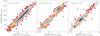 |
Fig. 7 Comparison of stellar mass estimates from our DESI VAC and COSMOS2020(FARMER; Weaver et al. 2022) catalog in three redshift bins. The 1:1 and ±0.2 dex lines are marked with black solid and dashed lines, respectively. The linear fit (red line) and the Pearson correlation coefficient are reported in the legend. |
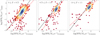 |
Fig. 8 Comparison of SFR estimates from our DESI VAC and COSMOS2020(FARMER; Weaver et al. 2022) catalog in three redshift bins. The 1:1 and ±0.2 dex lines are marked with black solid and dashed lines, respectively. The linear fit (red line) and the Pearson correlation coefficient are reported in the legend. |
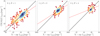 |
Fig. 9 Comparison of the bolometric AGN luminosity derived from the Chandra hard (2–7 keV band) X-ray luminosities of Suh et al. (2019) with those derived with CIGALE for a sample of 754 AGNs in three redshift bins. The 1:1 correlation is marked with a black solid line. The linear fit (red line) and the Pearson correlation coefficient are reported in the legend. |
5.2.2 DEVILS catalog
Thorne et al. (2022b) derived physical properties including stellar masses, SFR and AGN luminosities for ~500 000 DEVILS galaxies observed in the COSMOS field in the FUV – FIR using the PROSPECT SED fitting code incorporating AGN templates from Fritz et al. (2006) and flexible star formation and metallicity parameters (for details, see Thorne et al. 2022b and also Thorne et al. 2021, 2022a). PROSPECT identified 91% of BPT-selected AGNs and derived AGN luminosities in close agreement with the luminosities derived from Chandra X-ray (Marchesi et al. 2016). The AGN identification based on the PROSPECT code is based on the AGN fraction, requiring AGNFRAC > 0.1 (see also Table 2 in Thorne et al. 2022b for a comparison of PROSPECT AGN identification with standardly used techniques). We found PROSPECT counterparts for 5080 galaxies and we restricted our comparison to the sample of 1063 AGN and 2313 non-AGN galaxies with FIR photometry (FIRINPUT = 113) and an AGN fraction of AGNFRAC > 0.1 and ≤ 0.1, respectively. We find the median difference on the stellar mass estimates to be on the level Δ ~ −0.07 and NMAD ~0.17 for both AGN and non-AGN host galaxies. Further restricting the comparison to 386 AGNs with WISE photometry (FLAGINFRARED ≥ 3), we find the same AGN fraction (AGNFRACTIONDEVILS = 0.27 and AGNFRACTIONDESI = 0.26). This further highlights the independence of the estimates on the code and prescription used for deriving properties of galaxies.
6 Physical properties: model and photometry dependence
The SED fitting technique introduces several systematic uncertainties in derived properties coming from the assumptions made about the models, which may lead to a disagreement in the estimated stellar masses of up to a factor of ~2 (e.g., Maraston et al. 2006; Kannappan & Gawiser 2007; Conroy 2013; Lower et al. 2020; Pacifici et al. 2023). In this section, we consider how our choices of the SED modules (see Table 3) influence the main physical properties (stellar masses and SFRs). We validate the impact of the number of assumptions made about the IMF, fixed metallicity, SSP models, SFH prescription, dust attenuation and emission laws, and AGN models (see Table D.1 for a list of the changed parameters given in Appendix D). To quantify the effect, we made only one change, namely, in a parameter related to the default configuration (see Table 3). To discriminate the impact of the incorporation of the WISE photometry, we compared the physical properties estimated with or without WISE photometry or only with W1 and W2 bands in Sect. 6.4. Finally, we compared the CIGALE derived SFR with the ones estimated from the emission line measurement in Sect. 6.5. To preserve the computational time, we validated the influence of the model assumptions on a smaller sample of ~50 000 galaxies representing seven main galaxy classes: 1750 BL AGNs, 3900 NL AGNs, 8393 composite, 8819 star-forming, 8526 passive, 8846 retired, and 9962 other galaxies. The selection of this representative sample is described in Appendix D.1.
6.1 Stellar mass: choice of the stellar components
Stellar evolution models, such as Bruzual & Charlot (2003) or Maraston (2005), under the assumption of the IMF, describe the evolution of the SSP as a function of their stellar ages and metallicities following some fiducial SFH. In this section, we consider the dependence of the stellar masses on the choice of the i) IMF, ii) SSP models, iii) metallicity, and iv) SFH prescription.
We considered three main IMF choices: i) Salpeter (1955) assuming a power-law distribution with a heavier slope towards high-mass stars, ii) Kroupa (2001) assuming a broken power-law IMF with a shallower slope at higher stellar masses, implying fewer massive stars compared to Salpeter (1955), iii) Chabrier (2003), which combines a log-normal distribution for low-mass stars and a power-law distribution for higher masses and thus is considered as a reasonable middle ground between Salpeter (1955) and Kroupa (2001). The Chabrier (2003) IMF typically results in lower stellar mass estimates compared to the Salpeter (1955) IMF, because the Chabrier (2003) IMF reduces the contribution of high-mass stars, which are more massive and have a greater contribution to the total stellar mass. To mitigate the difference in stellar mass estimates we commonly assume a conversion factor between Chabrier (2003) and other IMFs, namely:
![Mathematical equation: $\[\begin{aligned}\mathrm{M}_{\star_{-}} \text {Salpeter } & =1.7 \cdot \mathrm{M}_{\star_{-}} \text {Chabrier, } \\\mathrm{M}_{\star_{-}} \text {Kroupa } & =1.1 \cdot \mathrm{M}_{\star_{-}} \text {Chabrier, }\end{aligned}\]$](/articles/aa/full_html/2024/11/aa51761-24/aa51761-24-eq20.png) (6)
(6)
as shown by, for instance, Cimatti et al. (2008), Longhetti & Saracco (2009), Bolzonella et al. (2010), and Ilbert et al. (2010). Here, we take the opportunity, to assess whether a simple scaling is sufficient and whether it varies for different types of galaxies. We find a constant median difference of -0.24 dex (see Sect. 5.1 for the definition of the median difference and Table 5 for the quantitative comparison of the estimates with different model assumptions) between stellar masses obtained assuming Chabrier (2003) and Salpeter (1955) stellar masses. This median difference is in agreement with the commonly used conversion factor and is independent of the stellar mass and galaxy class.
To generate the DESI VAC, we relied on the Bruzual & Charlot (2003) models. We discriminate the degree to which our estimates are different from the ones derived under the assumption of the Maraston (2005) model. The main difference between Maraston (2005) and Bruzual & Charlot (2003) relies on the incorporation of the thermally pulsating asymptotic giant branch (TP-AGB) stars in the evolution of galaxies in Maraston (2005) models. TP-AGB stars are evolved stars that can significantly affect the integrated light of galaxies, particularly in the NIR wavelength range. Due to the inclusion of TP-AGB stars, the Maraston (2005) model might yield higher stellar mass estimates compared to Bruzual & Charlot (2003) for galaxies with significant contributions from these stars, especially at intermediate and old ages (see more details in e.g., Maraston 2005; Conroy & Gunn 2010; Kriek et al. 2010; Maraston & Strömbäck 2011). While both models (BC03 and M05) include remnants, the exact mass contributions from remnants might not differ drastically between the two models. However, any differences would stem from the specific stellar evolution prescriptions and the IMF adopted in each model. The way these effects are included are not the same even for a simple Salpeter (1955) IMF (Maraston 2005) and some offsets just from that cannot be excluded (e.g., Maraston et al. 2013). Typically, remnants constitute a relatively small fraction of the total stellar mass, so while there might be differences, they should not be as pronounced as the differences arising from the TP-AGB treatment. We note that recent works using James Webb Telescope spectra reports the spectroscopic detection of the TP-AGB in galaxies at high-z and models with little contribution from that phase do not fit the data well (Lu et al. 2024). Different works have reported an offset of ~0.15 dex between stellar masses of Bruzual & Charlot (2003) and Maraston (2005) (e.g., Ilbert et al. 2010; Pozzetti et al. 2010; Kawinwanichakij et al. 2020). The change of the SSP model to Maraston (2005) introduces a median difference of −0.26 dex in our stellar mass estimates with respect to the ones derived with Bruzual & Charlot (2003) models. We refer to Sect. 5.1 for the definition of the median difference and Table 5 for the quantitative comparison of the estimates with different model assumptions.
Typically, physical properties are derived relying on the parametric SFHs, although they may suffer from strong biases in recovering the proper SFHs due to the assumption of the simplistic prescription (e.g., Ciesla et al. 2015; Carnall et al. 2019; Lower et al. 2020; Leja et al. 2022). As a response to the necessity of more advanced SFH prescription, non-parametric SFHs have been proposed (e.g., Leja et al. 2019; Lower et al. 2020; Ciesla et al. 2023). We verified how our stellar mass estimates change when using a non-parametric SFH module (sfhNlevels; see Table D.1) implemented in CIGALE (Ciesla et al. 2023). The formula of the non-parametric SFH is based on time bins in which the SFRs are constant and linked together by the bursty continuity (Tacchella et al. 2022), instead of the assumption of the analytical function. We refer the reader to Arango-Toro et al. (2023); Ciesla et al. (2024, 2023) for more details about the non-parametric SFH module. For DESI galaxies, the SED fitting of the optical-MIR photometry with non-parametric SFH has a negligible impact on the stellar mass estimates across the entire stellar mass range (with a median difference of 0.03). The median difference is two times higher for AGNs and star-forming galaxies (0.04–0.05) than for passive and retired galaxies (0.02; see Table 5).
Stellar metallicity is poorly constrained from photometric data alone due to the age-metallicity-dust degeneracy (e.g., Worthey 1994; Papovich et al. 2001). To overcome this problem, most commonly SED fitting-based approaches rely on fixing the metallictiy to a solar value (e.g., Małek et al. 2018; Boquien et al. 2019) or leaving it as a free but constant value over the lifetime of the galaxy (e.g., Carnall et al. 2018; Johnson et al. 2021). These assumptions may affect other parameters of interest, such as the stellar mass or SFRs introducing mass-dependent systematics (e.g., Pforr et al. 2012; Mitchell et al. 2013; Thorne et al. 2022a). On the other hand, other works (e.g., Osborne & Salim 2024) do not report the dependence of the stellar mass estimates on the choice of metallicity. We also validated the impact on the stellar mass estimates with models where the metallicity is allowed to vary (see Table D.1), instead of assuming the metallicity fixed to a solar value. For our catalog, allowing metallicity to vary introduces a median difference of −0.04 across the entire stellar mass range. The median difference is two times higher for NL AGNs and composite (−0.07) than for the remaining galaxy classes (−0.03; see Table 5).
6.2 Stellar mass: Choice of the dust models
We considered an alternate dust attenuation model proposed by Charlot & Fall 2000 (see Table D.1) to test the systematics. In contrast to Calzetti et al. (2000), this recipe assumes different attenuation for young (age < 10 Myr) and old stars (age > 10 Myr). Young stars are attenuated in the birth clouds, while both young and old stars are attenuated in the interstellar medium. In CIGALE, the implementation of the Charlot & Fall (2000) law is more flexible, giving the freedom to choose the values of input parameters (attenuation of the ISM, slopes of power-law attenuation curves for the birth cloud, and the ISM, and the ratio of the total attenuation). Both attenuation laws are modeled by a power law and normalized to the attenuation in the V band. The main difference in the shape of attenuation curves appears at λ>5000 Å, where Charlot & Fall (2000) is flatter than the one given by Calzetti et al. (2000). For example, Mitchell et al. (2013) estimated that the stellar mass can be underestimated by up to 0.6 dex by assuming the Calzetti et al. (2000) for massive galaxies. For DESI galaxies we find a median difference of −0.03 dex across the entire stellar mass range, but the median difference is higher for AGN and composite galaxies (Δ ~ −0.10) than for the remaining classes (Δ ~ −0.02; see Table 5).
We also considered the prescription of the dust emission model given by Dale et al. (2014) (see Table D.1), which is much simpler than the complex model of Draine et al. (2014). The star-forming component is described by dMd ∝ U−αdU, where Md is the dust mass heated by the radiation field at intensity U and α represents the relative contributions of the different local SEDs (Dale et al. 2014). The parameter α is the only free parameter and is tightly connected with the 60 − to − 100 μm color. Due to a limited variation of the PAH with respect to α, the model does have problems with proper modeling of the dust in metal-poor galaxies (e.g., Engelbracht et al. 2005). However, when using only optical-MIR SEDs, there is no difference in the used dust emission model, as indicated by the zero median difference in the stellar mass estimates using Dale et al. (2014) and Draine et al. (2014) prescriptions (see Sect. 5.1 for the definition of the median difference and Table 5 for the quantitative comparison of the estimates with different model assumptions).
6.3 Choice of the AGN models
Finally, we considered the impact of incorporating AGN templates on the stellar mass estimates by comparing the estimates from our VAC with estimates from CIGALE when the AGN contribution is fixed to 0 for the representative sample. As suggested by Thorne et al. (2022b), the inclusion of the AGN component is argued to be crucial not to overestimate the light coming from the host galaxies. However, our results suggest that the stellar masses for the general sample of galaxies are not affected significantly by the contribution of AGN as the median difference is low (Δ = 0.004 for the entire representative sample). On the other hand, the median difference is high for BL AGN (Δ = −0.26; see Fig. 10). This implies that the incorporation of the AGN models affects the stellar mass estimates (the median difference is slightly higher than the median stellar mass error; log(Mstar/M⊙)err = 0.23) for the BL AGNs; whereas for the remaining galaxy classes, this effect is negligible from the statistical point of view (i.e., the scatter shown in Fig. 10 is large if we consider the individual sources). We note that the difference in stellar mass for BL AGNs depends on redshift and stellar mass (see Fig. 11), while for the remaining classes, the stellar mass differences are independent of redshift and considered stellar mass range.
The change of the AGN model to the one proposed by Stalevski et al. (2012, 2016) (for the description of AGN models; see Sect. 3.4) does not affect the stellar mass estimates for the entire galaxy population (see Table 5) and the difference is the highest for the BL AGNs (with a median difference of 0.05 and NMAD of 0.14). However, we note that the scatter for individual galaxies is large; for individual sources, the masses might be higher even for 2–3 dex when using Fritz et al. (2006) models than when relying on Stalevski et al. (2012, 2016).
6.4 Stellar mass: choice of the photometry
Aside from the model assumptions discussed in the previous section, the SED coverage is one of the most important ingredients for deciding on the reliability of the SED-derived physical properties. The coverage of the FUV – FIR is highly desired to obtain reliable estimates of the contribution from young and old stars and AGNs (e.g., Thorne et al. 2022b,a). However, numerous works suggest that robust and reliable stellar mass estimates require only optical photometry to find the tight relation between optical color and stellar M/L ratio (e.g., Bell & de Jong 2001; Bell et al. 2003; Gallazzi & Bell 2009; Zibetti et al. 2009; Taylor et al. 2010). Gallazzi & Bell (2009) showed that stellar mass estimates obtained on one optical color are not biased against the estimates based on the optical-NIR SEDs or spectral features. However, Gallazzi & Bell (2009) based their estimates on the BC03 models that are NIR featureless. Other works instead find that only optical + NIR photometry can break the age, metallicity, and dust degeneracy (Maraston et al. 2010).
In this section, we compare the estimates of stellar mass for DESI galaxies assessing further in the wavelength, namely, using optical colors alone (grz) with the ones obtained based on the optical-MIR SED fit, adding i) only WISE1 and WISE2 (grzW12) and all four WISE photometry (grzW14). We find a negligible impact when incorporating W12 to the SED fit on the stellar mass estimates (Δ = −0.002; see Table 5) for the entire galaxy population. The discrepancy between stellar mass estimates increases for AGNs (Δ = 0.13 and −0.06 for BL and NL AGNs, respectively, and NMAD 0.26 and 0.16 for BL, and NL AGNs, respectively). Independently of the galaxy class, the scatter is large ±1 dex, thus the stellar masses for individual sources may differ significantly. The stellar masses obtained only based on grz photometry are still similar to the ones derived based on the grzW14 SED fits (Δ = 0.04), but the scatter increases (NMAD = 0.17; see Table 5). The degree of difference in stellar mass estimates depends on the galaxy types, and we find that this is higher for the BL AGNs (with Δ = 0.20 and NMAD = 0.34) than for the remaining classes (see Fig. 12). The difference in the stellar mass is independent of redshift except for the low redshift (Z ≲ 0.1), where the stellar mass estimated with WISE photometry are higher than the ones estimated only based on the optical bands (see Fig. 13). Independently of redshift, the stellar masses can differ up to ~1 dex for AGNs and composite galaxies – and even up to ~2 dex for star-forming and passive galaxies.
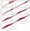 |
Fig. 10 Comparison of stellar mass estimates with or without incorporation of the AGN templates in SED fitting framework for the representative sample composed of seven different galaxy classes. The 1:1 and ±0.5 dex lines are marked with black solid and dashed lines, respectively. The linear fit (red line) and the Pearson correlation coefficient (r) are reported in the legend. The median difference (Δ) and NMAD are reported on the plots for each galaxy class (see Sect. 5.1 for the definition of the metric). |
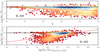 |
Fig. 11 Stellar mass difference between estimates obtained with and without incorporating AGN templates in the SED fitting for BL AGNs. The top panel shows the mass difference as a function of redshift, while the bottom panel displays it as a function of stellar mass. The black solid line represents zero mass difference, and the red dashed line corresponds to a linear fit to the data. |
6.5 SFR: Choice of the models and photometry
In this section, we validate how the SFRs are affected by the aforementioned choices in the SED framework. The SFR derived via SED fitting (SFR(SED)) depends on the wavelength coverage of the SED fits (e.g., the lack of FIR observations may alter its estimations (Ciesla et al. 2015). Thus, we used an alternative SFR indicator based on the Hα line luminosity (L(Hα)), following the definition given by Kennicutt (1998):
![Mathematical equation: $\[\operatorname{SFR}(\mathrm{H} \alpha)\left(\mathrm{M}_{\odot} \mathrm{yr}^{-1}\right)=7.9 \times 10^{-42} \mathrm{~L}(\mathrm{H} \alpha)(\mathrm{ergs}^{-1}),\]$](/articles/aa/full_html/2024/11/aa51761-24/aa51761-24-eq21.png) (7)
(7)
where L(Hα) is corrected for the dust extinction. In this work, we rely on the Balmer decrement method, which is commonly used to correct the line measurements for dust extinction through the comparison of the observed ratio of the Hα and Hβ emission lines (Robs) with the dust-free theoretical value (Rth = (Hα/Hβ)theoretical = 2.86; Groves et al. 2012). For the theoretical ratio, we used the case B (the optical thick limit) recombination, corresponding to a temperature of T = 104 K and electron density of Ne = 102 cm−3 (Osterbrock 1989). The Hα/Hβ ratio is linked with the attenuation at optical wavelengths by:
![Mathematical equation: $\[\mathrm{A}_{\mathrm{V}}=\mathrm{R}_{\mathrm{V}} \cdot 2.5 {\log} \left(\frac{\mathrm{R}_{\mathrm{obs}}}{\mathrm{R}_{\mathrm{th}}}\right) /\left(\mathrm{k}_{\mathrm{H} \beta}-\mathrm{k}_{\mathrm{H} \alpha}\right),\]$](/articles/aa/full_html/2024/11/aa51761-24/aa51761-24-eq22.png) (8)
(8)
where:
![Mathematical equation: $\[\begin{array}{r}\mathrm{k}_{\mathrm{H} \beta}=2.659 \times\left[-2.156+\left(1.509 / \lambda_{H \beta}\right)\right. \\\left.-\left(0.198 / \lambda_{H \beta}^2\right)+\left(0.011 / \lambda_{H \beta}^3\right)\right]+R_V,\end{array}\]$](/articles/aa/full_html/2024/11/aa51761-24/aa51761-24-eq23.png) (9)
(9)
![Mathematical equation: $\[\mathrm{k}_{\mathrm{H} \alpha}=2.659 \times\left[-1.857+\left(1.040 / \lambda_{\mathrm{H} \alpha}\right)\right]+\mathrm{R}_{\mathrm{V}},\]$](/articles/aa/full_html/2024/11/aa51761-24/aa51761-24-eq24.png) (10)
(10)
where RV = 4.05 (Calzetti et al. 2000), λHβ = 0.4861 μm and λHα = 0.6563 μm. The reddening is then expressed as:
![Mathematical equation: $\[\mathrm{E}(\mathrm{B}-\mathrm{V})=\mathrm{A}_{\mathrm{V}} / \mathrm{R}_{\mathrm{V}}.\]$](/articles/aa/full_html/2024/11/aa51761-24/aa51761-24-eq25.png) (11)
(11)
For the representative sample (see Appendix D.1 for the description of the representative sample), we selected galaxies with high S/N (S/N ≥ 3) of Hα and Hβ line fluxes taken from FastSpecFit v3.2 and correct the Hα for extinction following:
![Mathematical equation: $\[\mathrm{F}_{\text {corr }}=\mathrm{F}_{\text {observed }} \times 10^{0.4 \cdot \mathrm{k}_{\mathrm{H} \alpha} \cdot \mathrm{E}(\mathrm{B}-\mathrm{V})}.\]$](/articles/aa/full_html/2024/11/aa51761-24/aa51761-24-eq26.png) (12)
(12)
We also applied an aperture correction from FastSpecFit v3.2. Based on the corrected Hα flux and redshift, we derived the Hα luminosity; finally, we derived the SFR derived based on the Hα emission line (SFR(Hα)) following Eq. (7). To preserve the consistency of the IMF with the SFR definition proposed by Kennicutt (1998), we compared the SFR estimated with CIGALE assuming Salpeter (1955) IMF. We refer to Table 7 for the bias introduced by assumption of the Salpeter (1955) or Chabrier (2003) IMF). We show the comparison of the SFR(SED) and SFR(Hα) in Fig. 14 for the entire representative sample as well as for star-forming galaxies and AGNs. The discrepancy between SFR(SED) and SFR(Hα) given by Δ = 0.119 and NMAD = 0.567 (see Sect. 5.1 for the definitions of the metrics) are mostly driven by the AGN population. The SFRs for starforming galaxies are in closer agreement (Δ = 0.136 and NMAD = 0.413) than for AGNs (Δ = 0.248 and NMAD = 0.871). Table 6 shows how the Δ and NMAD changes with redshift. There are no clear trends, the consistency of the SFR(SED) and SFR(Hα) among different redshift bins suggests that there is no dependence on redshift. The consistency of SFR(SED) and SFR(Hα) for star-forming galaxies highlights the consistency of the SFRs derived based on the optical-MIR SEDs with the ones derived based on the emission lines.
The degree of the difference in our SFRs estimates from the ones derived by other prescriptions are quantified in Table 7 (see Sect. 5.1 for the definition of the metric). For the starforming galaxies, the bias introduced by the assumptions of the dust laws or AGN contribution does not significantly affect the SFR estimates (Δ and NMAD ≲ 0.1). The moderate differences (Δ and NMAD ≲ 0.3) are introduced by assumptions over IMF, SSP models, Z, or excluding W3 and W4 from SED fits, while the SFH or SED fits obtained solely on optical bands introduce large median differences and NMAD (Δ and NMAD ≳ 0.3). The agreement between SFR(SED) and SFR(Hα) degrades for AGNs, preserving only small Δ and NMAD for the choice of the AGN model (Δ and NMAD ≲ 0.1), while introducing large median difference and NMAD (Δ and NMAD ≳ 0.3) for SFH module and incorporating MIR information to SED fits. The rest of the assumptions introduced a moderate median difference.
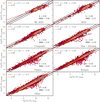 |
Fig. 12 Comparison of stellar mass estimates with or without incorporation of the MIR photometry to the SED fitting for the representative sample composed of seven different galaxy classes. The 1:1 and ±0.5 dex lines are marked with black solid and dashed lines, respectively. The linear fit (red line) and the Pearson correlation coefficient (r) are reported in the legend. The median difference (Δ) and NMAD (see Sect. 5.1 for the definition of the metric) are reported on the plots for each galaxy class: BL and NL AGNs, composite objects, starforming galaxies, passive and retired galaxies, and other sources. |
6.6 AGN features
As shown in the previous sections, the incorporation of the WISE photometry has an influence on the stellar mass and SFR estimates (see Sects. 6.4 and 6.5). Here, we explore how the AGN features derived with CIGALE depend on the inclusion of the MIR photometry in SED fits. The change of the AGN fraction (AGNFRAC) and viewing angle (AGNPSY) for the BL AGNs, NL AGNs, and star-forming galaxies drawn from the representative sample (see Appendix D.1 for a description of the representative sample) when using 1) solely optical information (grz), 2) optical and WISE W1 and W2 (grzW12), or 3) optical and all WISE (grzW14) is shown in Figs. 15 and 16, respectively. As expected, optical SED fits cannot distinguish the contribution of AGN to IR, which results in an artificial AGN fraction (AGNFRAC ~0.3) and viewing angle (AGNPSY ~35) for almost all galaxies independent of their galaxy type. The AGNFRAC and AGNPSY distributions start to differentiate for BL AGNs, NL AGNs, and star-forming galaxies when at least W12 is included in SED fitting. When the W12 is incorporated in the SED fits, the BL AGNs are characterized by lower AGNFRAC than NL AGNs (with a median AGNFRAC increasing from 0.16 to 0.24); whereas star-forming galaxies have an AGNFRAC distribution similar to that of NL AGN (with a median 0.22). Interestingly, when including W12, AGNPSY starts to properly identify BL AGNs based on their high viewing angle (AGNPSY ~80°), although there is also a strong peak at AGNPSY ~40°. Both star-forming and NL AGNs are characterized by similar viewing angles (AGNPSY ~40°).
The incorporation of all four WISE bands (W14) results in smoothing the AGNFRAC distribution for BL AGNs with a strong peak at AGNFRAC ~0.15 and AGNPSY ~80°; whereas for NL AGNs and star-forming galaxies, the distribution is characterized by a strong peak at AGNFRAC ~0 and a secondary peak at 0.25. The difference in AGNFRAC between star-forming and NL AGNs is in the long tail towards high values for NL AGNs, while the fraction of star-forming galaxies exceeding AGNFRAC ~0.35 is negligible. The AGNPSY distributions for NL AGNs and star-forming galaxies are similarly characterized by wide peaks at AGNPSY ~40°; however, a small fraction is characterized by the viewing angle typical for BL AGNs. Even with MIR SED fits, the distribution of AGNFRAC and AGNPSY for NL AGNs and star-forming galaxies are similar, challenging the usefulness of these AGN features to differentiate between AGN and non-AGN galaxies. Nevertheless, BL AGNs show a clear preference for AGNFRAC ~0.15 and AGNPSY ~80°.
Independently of the availability of WISE photometry, 80% of BL AGNs are identified as AGNs based on the AGNFRAC ≥ 0.1. Following the same criterion, 65% of NL AGNs are also classified as AGNs. A similar fraction (68%) of star-forming galaxies is characterized by AGNFRAC > 0.1, but this is reduced to 19% if all WISE bands with S/N ≥ 3 are included in the SED fits (FLAGINFRARED = 4). This confirms that without the MIR information, the star-forming galaxies overestimate the AGN contribution, although providing measurements in all four WISE bands reduces significantly the fraction of the star-forming galaxies with overestimated AGN fraction (from 68% to 19%).
The physical properties derived for the majority (68%) of star-forming galaxies are thus derived under the assumption of the false presence of AGN for sources without the MIR information. However, we validated the notion that the stellar mass estimates can still be securely used. For a sample of star-forming galaxies with AGNFRAC ≥ 0.1, we compared the derived stellar masses with the ones estimated without incorporating AGN contribution (i.e., the AGNFRAC is fixed to the null value) independently of the availability of WISE photometry. Both the Δ and NMAD are comparable (with Δ = 0.014 and NMAD = 0.037). Similarly, the effect on the SFR is negligible (Δ = -0.079 and NMAD = 0.119). For star-forming galaxies with a low AGN fraction (AGNFRAC ≤ 0.1), there is no impact on stellar mass or SFR estimates (with Δ = −0.001, −0.016 and NMAD = 0.011, 0.025 for stellar mass and SFR, respectively). To summarize, although the AGN features especially for sources lacking high S/N WISE photometry are not reliable, the overestimation of the AGN fraction for star-forming galaxies does not affect their stellar mass or SFR estimates.
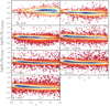 |
Fig. 13 Stellar mass difference between estimates obtained with and without incorporating WISE photometry in the SED fitting for seven different classes. Each panel shows the mass difference as a function of redshift with the black solid line representing zero mass difference and the red dashed line corresponding to a linear fit to the data. |
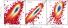 |
Fig. 14 Comparison of the SFR estimated from the Hα line with the SFR obtained from CIGALE optical-MIR SED fits for the entire representative sample (left panel), star-forming galaxies (middle panel)m and AGNs (BL and NL together; right panel). The 1:1 and ±0.2 dex lines are marked with black solid and dashed lines, respectively. |
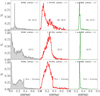 |
Fig. 15 Comparison of the AGNFRAC distribution obtained from SED fits incorporating grzW14 bands (left panels), grzW12 (middle panels), and solely grz bands (right panels) for BL AGNs (top panels), NL AGNs (middle panels), and star-forming galaxies (bottom panels) drawn from the representative sample (see Appendix D.1). The number of sources and the median AGNFRAC are reported in the plots. |
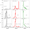 |
Fig. 16 Comparison of the AGNPSY distribution obtained from SED fits incorporating grzW14 bands (left panels), grzW12 (middle panels), and solely grz bands (right panels) for BL AGNs (top panels), NL AGNs (middle panels), and star-forming galaxies (bottom panels) drawn from the representative sample (see Appendix D.1). The number of sources and the median AGNFRAC are reported in the plots. |
7 Summary
We created the VAC of physical properties (including stellar masses, SFRs, rest-frame magnitudes, and AGN features) for DESI EDR galaxies. Here, we briefly summarize the VAC:
The catalog includes almost 1.3 million galaxies with optical and NIR photometry (grz) supplemented with WISE (W14) information spanning a broad redshift range (0.001 ≤ z ≤ 5.968; for details, see Sect. 2);
The physical properties are derived with the CIGALE SED fitting code (Boquien et al. 2019) including AGN templates from Fritz et al. (2006) (see Sect. 3 and Table 3 for details on the SED fitting prescription). Tables 5 and 7 elaborate on the extent to which our estimates depend on our model assumptions;
Several quality flags, such as the quality of the fit expressed by
![Mathematical equation: $\[\chi_{\mathrm{r}}^{2}\]$](/articles/aa/full_html/2024/11/aa51761-24/aa51761-24-eq27.png) , the PDF of the derived properties, or the S/N of available photometry, would allow users to adapt the sample to specific scientific goals (see Sect. 4.1);
, the PDF of the derived properties, or the S/N of available photometry, would allow users to adapt the sample to specific scientific goals (see Sect. 4.1);We identified red and blue BGS galaxies based on the UVJ diagram (Whitaker et al. 2012) and revised their location on the star-forming MS (see Sect. 4.2);
We evaluated the bias and deviations introduced by several model parameters, including SSP, SFH, and dust choice, on stellar mass (see Sect. 6 and Table 5) and SFR (see Sect. 6.5 and Table 7);
We found a very good agreement with COSMOS and other VACs that are BC03-based. The relatively good agreement with the SDSS(Firefly) VAC, which is obtained by fitting the spectra, rather than the photometry. Using another model prescription (SSP, SFH, metallicities, etc.) showcases the excellent agreement of the stellar mass estimates with other VACs (see Sect. 5 and Table 4).
The VAC presented here highlights the importance of incorporating MIR photometry in the SED fits. Without the inclusion of WISE photometry, the AGN fraction would be overestimated for star-forming galaxies, although it does not affect their stellar mass or SFR estimates (see Sect. 6.6). We demonstrate that accounting for the AGN contribution is essential for deriving stellar masses for galaxies hosting AGN. With CIGALE, we are able to recover both stellar masses and AGN luminosities in a way that is consistent with other methods. We note that the particular host properties of DESI AGNs will be explored in detail in a future work.
Acknowledgements
The presented analysis is conducted on the VAC of physical properties of DESI galaxies v1.2, while the latest available version v1.4 includes an additional 51126 (4%) that were missing information about the RELEASE in the previous version. There is also a supplementary table of 8422 sources for which physical properties are based on the redshift coming from the QSO afterbruner pipeline relying on the QuasrNet and the broad Mg II finder pipelines. The afterburner shows better performance (94%) in identifying visually inspected QSOs relative to Redrock pipeline (86%; see Chaussidon et al. 2023 and Alexander et al. 2023 for more details). The VAC for the forthcoming release (DESI Year 1) will be published as part of Data Release 1 similar to the currently public DESI EDR. The authors thank the anonymous referee for insightful comments. The authors would like to express their appreciation to Laure Ciesla for sharing the CIGALE non-parametric SFH module sfhNlevels, J. Thorne, and H. Suh for sharing their catalogs. This work has been supported by the Polish National Agency for Academic Exchange (Bekker grant BPN/BEK/2021/1/00298/DEC/1) and the European Union’s Horizon 2020 Research and Innovation program under the Maria Sklodowska-Curie grant agreement (No. 754510). M.S. acknowledges financial support from the State Research Agency of the Spanish Ministry of Science and Innovation under the grants ‘Galaxy Evolution with Artificial Intelligence’ with reference PGC2018-100852-A-I00 and ’BASALT’ with reference PID2021-126838NB-I00. M.M. acknowledges support from the Spanish Ministry of Science and Innovation through the project PID2021-124243NB-C22. This work was partially supported by the program Unidad de Excelencia María de Maeztu CEX2020-001058-M. H.Z. acknowledges the support from the National Natural Science Foundation of China (NSFC; grant Nos. 12120101003 and 12373010) and National Key R&D Program of China (grant Nos. 2023YFA1607800, 2022YFA1602902) and Strategic Priority Research Program of the Chinese Academy of Science (Grant Nos. XDB0550100). This material is based upon work supported by the U.S. Department of Energy (DOE), Office of Science, Office of High-Energy Physics, under Contract No. DE–AC02–05CH11231, and by the National Energy Research Scientific Computing Center, a DOE Office of Science User Facility under the same contract. Additional support for DESI was provided by the U.S. National Science Foundation (NSF), Division of Astronomical Sciences under Contract No. AST-0950945 to the NSF’s National Optical-Infrared Astronomy Research Laboratory; the Science and Technology Facilities Council of the United Kingdom; the Gordon and Betty Moore Foundation; the Heising-Simons Foundation; the French Alternative Energies and Atomic Energy Commission (CEA); the National Council of Humanities, Science and Technology of Mexico (CONAHCYT); the Ministry of Science, Innovation and Universities of Spain (MICIU/AEI/10.13039/501100011033), and by the DESI Member Institutions: https://www.desi.lbl.gov/collaborating-institutions. Any opinions, findings, and conclusions or recommendations expressed in this material are those of the author(s) and do not necessarily reflect the views of the U.S. National Science Foundation, the U. S. Department of Energy, or any of the listed funding agencies. The authors are honored to be permitted to conduct scientific research on Iolkam Du’ag (Kitt Peak), a mountain with particular significance to the Tohono O’odham Nation. The DESI Legacy Imaging Surveys consist of three individual and complementary projects: the Dark Energy Camera Legacy Survey (DECaLS), the Beijing-Arizona Sky Survey (BASS), and the Mayall z-band Legacy Survey (MzLS). DECaLS, BASS and MzLS together include data obtained, respectively, at the Blanco telescope, Cerro Tololo Inter-American Observatory, NSF’s NOIRLab; the Bok telescope, Steward Observatory, University of Arizona; and the Mayall telescope, Kitt Peak National Observatory, NOIRLab. NOIRLab is operated by the Association of Universities for Research in Astronomy (AURA) under a cooperative agreement with the National Science Foundation. Pipeline processing and analyses of the data were supported by NOIRLab and the Lawrence Berkeley National Laboratory. Legacy Surveys also uses data products from the Near-Earth Object Wide-field Infrared Survey Explorer (NEOWISE), a project of the Jet Propulsion Laboratory/California Institute of Technology, funded by the National Aeronautics and Space Administration. Legacy Surveys was supported by: the Director, Office of Science, Office of High Energy Physics of the U.S. Department of Energy; the National Energy Research Scientific Computing Center, a DOE Office of Science User Facility; the U.S. National Science Foundation, Division of Astronomical Sciences; the National Astronomical Observatories of China, the Chinese Academy of Sciences and the Chinese National Natural Science Foundation. LBNL is managed by the Regents of the University of California under contract to the U.S. Department of Energy. The complete acknowledgments can be found at https://www.legacysurvey.org/.
Data availability
The VAC of physical properties of DESI galaxies is publicly available at https://data.desi.lbl.gov/doc/releases/edr/vac/cigale/. The data behind the figures are available at https://doi.org/10.5281/zenodo.13847488.
A copy of the catalog is available at the CDS via anonymous ftp to cdsarc.cds.unistra.fr (130.79.128.5) or via https://cdsarc.cds.unistra.fr/viz-bin/cat/J/A+A/691/A308.
Appendix A Catalog structure
A description of the columns in the catalog is given in Table A.1.
Data model of the DESI VAC.
Appendix B Stellar mass errors dependence on the quality of the photometry
The errors in the stellar mass and SFR estimates depend on the model assumptions done for the SED fitting and on the spectral coverage included in the SED fits. Standardly, the logarithmic stellar masses are constrained to the 0.2 − 0.4 dex level (e.g., Conroy 2013; Comparat et al. 2017; Pacifici et al. 2023) depending on the assumptions on the SFH, IMF and other model prescriptions (for our stellar mass estimates the dependence on model assumptions is outlined in Sect. 6). For our stellar mass estimates, there is a clear dependence of the uncertainties on the S/N of the input photometry (see Fig. B.1). An accuracy level of ≲ 0.25 dex for galaxies is fulfilled when the g, r, z observations have S/N ≥ 10. In the case of QSO, an accuracy limit of ≲ 0.20 dex is achieved with at least 3 WISE bands measured with S/N ≥ 7 (independently of the optical measurements). We note that the errors increase with redshift, implying for QSO at z > 1.5 that even with high S/N the errors may reach ~ 0.8 dex (see the blue tail in the left plot in Fig. B.1).
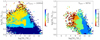 |
Fig. B.1 Dependence of the stellar mass error (log(Mstar/M⊙)err) on the stellar mass (log(Mstar/M⊙)) for two main DESI types: GALAXIES (left panel) and QSOs (right panel). The stellar mass uncertainties depend on the S/N of the optical (igrz) photometry (left panel) as well as on the S/N of the WISE photometry (right panel). The low errors (log(Mstar/M⊙)err ≲ 0.25) are achieved when at least 3 optical bands are observed with S/N ≥ 10 and at least 3 WISE bands are measured with S/N ≥ 7. |
Appendix C Comparison with other catalogs
In this appendix, we further explore the comparison of the stellar mass obtained with CIGALE for DESI EDR galaxies with the reference catalogs. In Sect. 5, we offer a comparison of stellar masses drawn from the COSMOS2020 catalog and AGN and host properties based on the samples overlapping with AGN-COSMOS catalogs. Here, we expand the comparison of the stellar masses with the SDSS(FIREFLY) and SDSS(MPA-JHU) catalogs (Sect. C.1), with the GSWLC (Sect. C.2) and with the DESI catalog presented by Zou et al. 2024 (Sect. C.3).
C.1 SDSS
To date, the largest spectroscopic survey, SDSS, had provided several VACs including estimates of the stellar properties. In this work, we compare our stellar mass estimates derived with CIGALE with two commonly used SDSS catalogs: i) eBOSS SDSS FIREFLY DR16 SDSS(FIREFLY)14 (Comparat et al. 2017), and ii) MPA-JHU DR815 (Kauffmann et al. 2003b; Brinchmann et al. 2004; Tremonti et al. 2004). The SDSS(Firefly) catalog provides stellar properties (age, metallicity, dust reddening, stellar mass, and the SFH) obtained through a comprehensive analysis of the galaxy spectra from SDSS, Baryon Oscillation Spectroscopic Survey (BOSS), and eBOSS. The physical properties were inferred via full spectral fitting with the chi-squared minimization fitting code FIREFLY (Wilkinson et al. 2017). The catalog relies on the stellar population models from Maraston & Strömbäck (2011) utilizing different stellar libraries and IMFs. In this work, we use the stellar masses obtained assuming a Chabrier (2003) IMF and using the MILES libraries (Sánchez-Blázquez et al. 2006; Beifiori et al. 2011; Falcón-Barroso et al. 2011). The SDSS(MPA-JHU) catalog is a VAC of physical properties of SDSS DR8 galaxy derived from fitting their photometry. The catalog provides line measurements, Lick, and other indices as well as the physical properties. The stellar masses and SFRs are derived from the SED fitting (covering ugriz) using the models and methodology outlined in Kauffmann et al. (2003a). To avoid the aperture effect on the stellar mass estimates, these are derived based on the photometry rather than the spectral indices as originally proposed by Kauffmann et al. (2003a). The SED fitting relies on templates generated with Bruzual & Charlot (2003) SSP models and a Kroupa (2001) IMF. The catalog includes the stellar mass measurements corresponding to the median and 2.5%, 16%, 84%, and 97.5% of the PDF.
The comparison of the DESI stellar masses derived with CIGALE with SDSS stellar masses for the galaxies in the overlap between the samples is shown in Fig. C.1 and the metrics are presented in Table 4. There is a good agreement between our stellar masses with SDSS(MPA-JHU), with a small median difference and NMAD (Δ = −0.071; NMAD = 0.126) that increases when comparing to the SDSS(FIREFLY) estimates, which is the only one characterized by a positive median difference. This comparison suggests that the SDSS(FIREFLY) stellar mass might be underestimated by an average of 0.2 dex for massive galaxies (log(Mstar/M⊙) ~ 11; see the left panel in Fig. C.1) as their stellar masses are derived from spectra with apertures that do not cover the full galaxies. On the contrary, for the SDSS(MPA-JHU) we find a close agreement across the entire mass range.
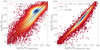 |
Fig. C.1 Comparison of our DESI stellar mass estimates with 24,947 and 18,778 stellar mass estimates from the SDSS(FIREFLY) (left panel) and the SDSS(MPA-JHU) catalogs (right panel), respectively. The 1:1 and 0.2 dex lines are marked with black solid and dashed lines, respectively. The linear fit (red line) and the Pearson correlation coefficient are reported in the legend. |
C.2 GSWLC
In this work, we use the GSWLC X2 catalog (Salim et al. 2018), an updated version of the GSWLC 1 version (Salim et al. 2016). The catalog includes physical properties derived for more than 650,000 galaxies covering 90% of SDSS with the CIGALE SED fitting code. The updated version modifies the energy balance in the SED fitting by using luminosity-dependent IR templates to derive the total IR luminosity from W3 or W4 photometry to derive more accurate SFRs. For SDSS sources classified as AGN based on the BPT diagram (Tremonti et al. 2004), the IR luminosity is corrected before SED fitting (see details in Salim et al. 2018). The GSWLC 2 catalog is based on the Chabrier (2003) and Bruzual & Charlot (2003) SSP models. For the sample of 17,902 DESI galaxies matched with the GSWLC 2 catalog, we find a good agreement between the stellar masses across the full stellar mass range with an offset of the 0.2 dex towards lower estimates for our measurements (see Fig. C.2). Although both catalogs rely on the CIGALE, the dust attenuation and energy balance are different and could explain the offset. Interestingly, the scatter of the stellar mass estimates is correlated with the quality of the WISE photometry (see lower panel in Fig. C.2). Sources observed with at least 2 WISE bands with S/N > 3 are characterized by a larger spread. The investigation of this relation is left for future work on the comparison of different stellar mass estimates for DESI galaxies.
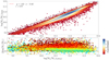 |
Fig. C.2 Comparison of ~18,000 stellar mass estimates from our VAC and GSWLC 2 catalogs (top panel) and difference in stellar mass estimates (bottom panel). The 1:1 and 0.2 dex lines are marked with black solid and dashed lines, respectively. The linear fit (red line) and the Pearson correlation coefficient are reported in the legend. The bottom panel shows the dependence of the stellar mass residuals on the availability of WISE photometry expressed by FLAGINFRARED: the scatter increases when WISE photometry is readily available. |
C.3 DESI catalogs
The comparison of stellar masses across different VACs built for DESI galaxies will be discussed in future work. We restrict here the comparison to the stellar mass estimates obtained by Zou et al. (2024). Both VACs rely on CIGALE estimates with the same SSP models and IMF, however, they differ in the prescription, e.g: Zou et al. (2024) leave stellar metallicity as a free parameter, while in our catalog it is fixed to a solar value and our catalog accounts for the AGN templates. We compare separately stellar masses for 125,077 star-forming and 9,852 AGN galaxies selected based on the [N II] Baldwin, Phillips, and Terlevich diagram (BPT Baldwin et al. 1981). The discrepancy between stellar mass measurements is higher for AGNs than for star-forming galaxies (median difference increases from −0.136 to −0.199 and NMAD from 0.211 to 0.303). The comparison of the stellar mass estimates is shown in Fig. C.3.
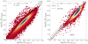 |
Fig. C.3 Comparison of our stellar masses with the estimates from Zou et al. (2024) for [N II] BPT-selected star-forming galaxies (left panel) and AGNs(right panel). The 1:1 and 0.2 dex lines are marked with black solid and dashed lines, respectively. The linear fit (red line) and the Pearson correlation coefficient are reported in the legend. The discrepancies between stellar masses are larger for AGNs than for star-forming galaxies. |
Appendix D SED fitting modules
As outlined in Sect. 6, we quantified the effect of the model assumptions for the stellar mass estimates on the representative sample of EDR galaxies described in the following App. D.1. The priors of the SED fitting modules we analyzed are summarized in Table D.1.
D.1 Representative sample selection
To analyze the influence of the assumptions made to generate models and the incorporation of the MIR photometry to the SED fitting on the main physical properties of DESI galaxies (stellar masses and SFRs), we select a representative sample of 50,196 sources. The sample consists of seven different galaxy types: BL AGNs, NL AGNs, composite objects, star-forming galaxies, passive galaxies, retired galaxies, and others. To select the representative sample we restrict the sample of 1,286,124 EDR galaxies (see Sect. 2) to 512,002 sources (GALAXIES and QSOs) spanning out to redshift z = 0.5 where Hα is visible in DESI spectra. The galaxy selection is based on the emission line measurements coming from FastSpecFit v2.0 (Moustakas et al. 2023; Moustakas in prep.). The selection of 1,750 BL AGNs is based on the Hα line requiring that the amplitude of the narrow and broad components have high S/N (S/N NHALPHA_BROAD_AMP ≥ 3, S/NHALPHA_NARROW_AMP ≥ 3) and that the 2-component Gaussian fit is favored over a single fit by χ2 (Δχ2 ≥ 0). From the remaining set, NL AGNs, composite, and star-forming galaxies are identified based on the [N II] BPT diagram requiring high S/N for the amplitudes of the lines used in the [N II] BPT diagram (S/NHALPHA_AMP ≥ 3, S/NHBETA_AMP ≥ 3, S/N[0III]λ5007_AMP ≥ 3). Following the selection proposed by Kewley et al. (2001) and Kauffmann et al. (2003a), we select 3,900 NL AGNs, 8,393 composite, and 101,757 star-forming galaxies. Among the remaining set of galaxies (396,202) we select 47,797 passive galaxies following the criterion based on the equivalent width of the Hα line:
![Mathematical equation: $\[0<\text { HALPHA_EW < Q. } 5 ~\AA,\]$](/articles/aa/full_html/2024/11/aa51761-24/aa51761-24-eq29.png) (D.1)
(D.1)
and 63,486 retired galaxies based on the cut:
![Mathematical equation: $\[0.5 \leq \text { HALPHA_EW } \leq 5 ~\AA\.]$](/articles/aa/full_html/2024/11/aa51761-24/aa51761-24-eq30.png) (D.2)
(D.2)
Sources that did not match any of the above criteria (284,919) are kept as others. Among all the galaxy classes, except for AGNs and composite, we randomly select sources in different bins of absolute z magnitude (ABSMAG_SDSS_Z)-redshift (Z) space. The summary of the composition of the representative sample is given in Table D.2.
D.2 The reliability of the fit
The goodness of the fit is quantified by the reduced χ2 of the best-fitting model (![Mathematical equation: $\[\chi_{r}^{2}\]$](/articles/aa/full_html/2024/11/aa51761-24/aa51761-24-eq31.png) ). In principle, one would expect a good fit with
). In principle, one would expect a good fit with ![Mathematical equation: $\[\chi_{r}^{2}=1\]$](/articles/aa/full_html/2024/11/aa51761-24/aa51761-24-eq32.png) , as
, as ![Mathematical equation: $\[\chi_{r}^{2}>1\]$](/articles/aa/full_html/2024/11/aa51761-24/aa51761-24-eq33.png) indicates issues in fully capturing the data, and
indicates issues in fully capturing the data, and ![Mathematical equation: $\[\chi_{r}^{2}<1\]$](/articles/aa/full_html/2024/11/aa51761-24/aa51761-24-eq34.png) points to overfitting. However, since the models are highly non-linear, it is almost impossible to correctly quantify the number of degrees of freedom for each galaxy (Andrae et al. 2010; Chevallard & Charlot 2016), and thus
points to overfitting. However, since the models are highly non-linear, it is almost impossible to correctly quantify the number of degrees of freedom for each galaxy (Andrae et al. 2010; Chevallard & Charlot 2016), and thus ![Mathematical equation: $\[\chi_{r}^{2}\]$](/articles/aa/full_html/2024/11/aa51761-24/aa51761-24-eq35.png) in CIGALE corresponds to the χ2 divided by the total number of input fluxes (instead of number of freedom in its statistical definition). Therefore, we follow the commonly used approach of removing the bad fits by sigma-clipping the
in CIGALE corresponds to the χ2 divided by the total number of input fluxes (instead of number of freedom in its statistical definition). Therefore, we follow the commonly used approach of removing the bad fits by sigma-clipping the ![Mathematical equation: $\[\chi_{\mathrm{r}}^{2}\]$](/articles/aa/full_html/2024/11/aa51761-24/aa51761-24-eq36.png) (e.g., Małek et al. 2018) and keep only those galaxies for which
(e.g., Małek et al. 2018) and keep only those galaxies for which ![Mathematical equation: $\[\chi_{\mathrm{r}}^{2}\]$](/articles/aa/full_html/2024/11/aa51761-24/aa51761-24-eq37.png) ≤ 17, which corresponds to ~95% of the sample. This threshold is also dictated by our visual inspection of the quality of the SED fitting, where we find a degradation of the fitting of the MIR part of the spectrum. We note that in the literature more restrictive cuts (
≤ 17, which corresponds to ~95% of the sample. This threshold is also dictated by our visual inspection of the quality of the SED fitting, where we find a degradation of the fitting of the MIR part of the spectrum. We note that in the literature more restrictive cuts (![Mathematical equation: $\[\chi_{\mathrm{r}}^{2} \leq 5\]$](/articles/aa/full_html/2024/11/aa51761-24/aa51761-24-eq38.png) ) are adapted for the scientific analysis and we encourage the user to use the one more appropriate for their scientific case (e.g., Buat et al. 2021).
) are adapted for the scientific analysis and we encourage the user to use the one more appropriate for their scientific case (e.g., Buat et al. 2021).
Alternative parameters used in SED fitting with CIGALE.
Composition of the representative DESI sample drawn from 1,286,124 EDR galaxies.
References
- Abdurro’uf, Lin, Y.-T., Wu, P.-F., & Akiyama, M. 2021, ApJS, 254, 15 [CrossRef] [Google Scholar]
- Acquaviva, V., Raichoor, A., & Gawiser, E. 2015, ApJ, 804, 8 [NASA ADS] [CrossRef] [Google Scholar]
- Alexander, D. M., Davis, T. M., Chaussidon, E., et al. 2023, AJ, 165, 124 [NASA ADS] [CrossRef] [Google Scholar]
- Almeida, A., Anderson, S. F., Argudo-Fernández, M., et al. 2023, ApJS, 267, 44 [NASA ADS] [CrossRef] [Google Scholar]
- Anand, A., Guy, J., Bailey, S., et al. 2024, AJ, 168, 124 [NASA ADS] [CrossRef] [Google Scholar]
- Andrae, R., Schulze-Hartung, T., & Melchior, P. 2010, arXiv e-prints [arXiv:1012.3754] [Google Scholar]
- Arango-Toro, R. C., Ciesla, L., Ilbert, O., et al. 2023, A&A, 675, A126 [NASA ADS] [CrossRef] [EDP Sciences] [Google Scholar]
- Arnouts, S., Moscardini, L., Vanzella, E., et al. 2002, MNRAS, 329, 355 [Google Scholar]
- Arnouts, S., Le Floc’h, E., Chevallard, J., et al. 2013, A&A, 558, A67 [NASA ADS] [CrossRef] [EDP Sciences] [Google Scholar]
- Assef, R. J., Stern, D., Kochanek, C. S., et al. 2013, ApJ, 772, 26 [Google Scholar]
- Bailey, S. 2012, PASP, 124, 1015 [NASA ADS] [CrossRef] [Google Scholar]
- Baldry, I. K., Liske, J., Brown, M. J. I., et al. 2018, MNRAS, 474, 3875 [Google Scholar]
- Baldwin, J. A., Phillips, M. M., & Terlevich, R. 1981, PASP, 93, 5 [Google Scholar]
- Barrows, R. S., Comerford, J. M., Stern, D., & Assef, R. J. 2021, ApJ, 922, 179 [NASA ADS] [CrossRef] [Google Scholar]
- Beifiori, A., Maraston, C., Thomas, D., & Johansson, J. 2011, A&A, 531, A109 [NASA ADS] [CrossRef] [EDP Sciences] [Google Scholar]
- Bell, E. F., & de Jong, R. S. 2001, ApJ, 550, 212 [Google Scholar]
- Bell, E. F., McIntosh, D. H., Katz, N., & Weinberg, M. D. 2003, ApJS, 149, 289 [Google Scholar]
- Best, P. N., Kondapally, R., Williams, W. L., et al. 2023, MNRAS, 523, 1729 [NASA ADS] [CrossRef] [Google Scholar]
- Bichang’a, B., Kaviraj, S., Lazar, I., et al. 2024, MNRAS, 532, 613 [CrossRef] [Google Scholar]
- Bolzonella, M., Kovač, K., Pozzetti, L., et al. 2010, A&A, 524, A76 [NASA ADS] [CrossRef] [EDP Sciences] [Google Scholar]
- Boquien, M., Duc, P. A., Galliano, F., et al. 2010, AJ, 140, 2124 [NASA ADS] [CrossRef] [Google Scholar]
- Boquien, M., Burgarella, D., Roehlly, Y., et al. 2019, A&A, 622, A103 [NASA ADS] [CrossRef] [EDP Sciences] [Google Scholar]
- Bouché, N., Dekel, A., Genzel, R., et al. 2010, ApJ, 718, 1001 [Google Scholar]
- Bowman, W. P., Zeimann, G. R., Nagaraj, G., et al. 2020, ApJ, 899, 7 [NASA ADS] [CrossRef] [Google Scholar]
- Brammer, G. B., van Dokkum, P. G., & Coppi, P. 2008, ApJ, 686, 1503 [Google Scholar]
- Brinchmann, J., Charlot, S., White, S. D. M., et al. 2004, MNRAS, 351, 1151 [Google Scholar]
- Bruzual, G., & Charlot, S. 2003, MNRAS, 344, 1000 [NASA ADS] [CrossRef] [Google Scholar]
- Buat, V., Ciesla, L., Boquien, M., Małek, K., & Burgarella, D. 2019, A&A, 632, A79 [NASA ADS] [CrossRef] [EDP Sciences] [Google Scholar]
- Buat, V., Mountrichas, G., Yang, G., et al. 2021, A&A, 654, A93 [NASA ADS] [CrossRef] [EDP Sciences] [Google Scholar]
- Burke, C. J., Liu, X., Shen, Y., et al. 2022, MNRAS, 516, 2736 [NASA ADS] [CrossRef] [Google Scholar]
- Burke, C. J., Liu, Y., Ward, C. A., et al. 2024, ApJ, 971, 140 [NASA ADS] [CrossRef] [Google Scholar]
- Calistro Rivera, G., Lusso, E., Hennawi, J. F., & Hogg, D. W. 2016, ApJ, 833, 98 [Google Scholar]
- Calzetti, D., Armus, L., Bohlin, R. C., et al. 2000, ApJ, 533, 682 [NASA ADS] [CrossRef] [Google Scholar]
- Carnall, A. C., McLure, R. J., Dunlop, J. S., & Davé, R. 2018, MNRAS, 480, 4379 [Google Scholar]
- Carnall, A. C., Leja, J., Johnson, B. D., et al. 2019, ApJ, 873, 44 [Google Scholar]
- Casey, C. M. 2012, MNRAS, 425, 3094 [Google Scholar]
- Chabrier, G. 2003, PASP, 115, 763 [Google Scholar]
- Charlot, S., & Fall, S. M. 2000, ApJ, 539, 718 [Google Scholar]
- Chaussidon, E., Yèche, C., Palanque-Delabrouille, N., et al. 2023, ApJ, 944, 107 [NASA ADS] [CrossRef] [Google Scholar]
- Chevallard, J., & Charlot, S. 2016, MNRAS, 462, 1415 [NASA ADS] [CrossRef] [Google Scholar]
- Ciesla, L., Charmandaris, V., Georgakakis, A., et al. 2015, A&A, 576, A10 [NASA ADS] [CrossRef] [EDP Sciences] [Google Scholar]
- Ciesla, L., Elbaz, D., & Fensch, J. 2017, A&A, 608, A41 [NASA ADS] [CrossRef] [EDP Sciences] [Google Scholar]
- Ciesla, L., Gómez-Guijarro, C., Buat, V., et al. 2023, A&A, 672, A191 [NASA ADS] [CrossRef] [EDP Sciences] [Google Scholar]
- Ciesla, L., Elbaz, D., Ilbert, O., et al. 2024, A&A, 686, A128 [NASA ADS] [CrossRef] [EDP Sciences] [Google Scholar]
- Cimatti, A., Cassata, P., Pozzetti, L., et al. 2008, A&A, 482, 21 [NASA ADS] [CrossRef] [EDP Sciences] [Google Scholar]
- Comparat, J., Maraston, C., Goddard, D., et al. 2017, arXiv e-prints [arXiv:1711.06575] [Google Scholar]
- Conroy, C. 2013, ARA&A, 51, 393 [NASA ADS] [CrossRef] [Google Scholar]
- Conroy, C., & Gunn, J. E. 2010, ApJ, 712, 833 [Google Scholar]
- Conselice, C. J., Singh, M., Adams, N., et al. 2023, MNRAS, 525, 1353 [CrossRef] [Google Scholar]
- Cooper, A. P., Koposov, S. E., Allende Prieto, C., et al. 2023, ApJ, 947, 37 [NASA ADS] [CrossRef] [Google Scholar]
- Csizi, B., Tortorelli, L., Siudek, M., et al. 2024, A&A, 689, A37 [NASA ADS] [CrossRef] [EDP Sciences] [Google Scholar]
- da Cunha, E., Charlot, S., & Elbaz, D. 2008, MNRAS, 388, 1595 [Google Scholar]
- Daddi, E., Bournaud, F., Walter, F., et al. 2010, ApJ, 713, 686 [NASA ADS] [CrossRef] [Google Scholar]
- Dale, D. A., Helou, G., Magdis, G. E., et al. 2014, ApJ, 784, 83 [Google Scholar]
- Darragh-Ford, E., Wu, J. F., Mao, Y.-Y., et al. 2023, ApJ, 954, 149 [CrossRef] [Google Scholar]
- Davé, R., Katz, N., Oppenheimer, B. D., Kollmeier, J. A., & Weinberg, D. H. 2013, MNRAS, 434, 2645 [CrossRef] [Google Scholar]
- Davies, L. J. M., Driver, S. P., Robotham, A. S. G., et al. 2016, MNRAS, 461, 458 [NASA ADS] [CrossRef] [Google Scholar]
- Davies, L. J. M., Thorne, J. E., Robotham, A. S. G., et al. 2021, MNRAS, 506, 256 [NASA ADS] [CrossRef] [Google Scholar]
- Davies, L. J. M., Thorne, J. E., et al. 2024, MNRAS, submitted [Google Scholar]
- de Barros, S., Schaerer, D., & Stark, D. P. 2014, A&A, 563, A81 [NASA ADS] [CrossRef] [EDP Sciences] [Google Scholar]
- DESI Collaboration (Aghamousa, A., et al.) 2016a, arXiv e-prints [arXiv:1611.00036] [Google Scholar]
- DESI Collaboration (Aghamousa, A., et al. 2016b, arXiv e-prints [arXiv:1611.00037] [Google Scholar]
- DESI Collaboration (Abareshi, B., et al.) 2022, AJ, 164, 207 [NASA ADS] [CrossRef] [Google Scholar]
- DESI Collaboration (Adame, A. G., et al.) 2024a, AJ, 168, 58 [NASA ADS] [CrossRef] [Google Scholar]
- DESI Collaboration (Adame, A. G., et al.) 2024b, AJ, 167, 62 [NASA ADS] [CrossRef] [Google Scholar]
- DESI Collaboration (Adame, A. G., et al.) 2024c, arXiv e-prints [arXiv:2404.03002] [Google Scholar]
- DESI Collaboration (Adame, A. G., et al.) 2024d, arXiv e-prints [arXiv:2404.03001] [Google Scholar]
- DESI Collaboration (Adame, A. G., et al.) 2024e, arXiv e-prints [arXiv:2404.03000] [Google Scholar]
- Dey, A., Schlegel, D. J., Lang, D., et al. 2019, AJ, 157, 168 [Google Scholar]
- Donevski, D., Lapi, A., Małek, K., et al. 2020, A&A, 644, A144 [NASA ADS] [CrossRef] [EDP Sciences] [Google Scholar]
- Doore, K., Monson, E. B., Eufrasio, R. T., et al. 2023, ApJS, 266, 39 [NASA ADS] [CrossRef] [Google Scholar]
- Draine, B. T., & Li, A. 2007, ApJ, 657, 810 [CrossRef] [Google Scholar]
- Draine, B. T., Aniano, G., Krause, O., et al. 2014, ApJ, 780, 172 [Google Scholar]
- Durodola, E., Pacucci, F., & Hickox, R. C. 2024, arXiv e-prints [arXiv:2406.10329] [Google Scholar]
- Elbaz, D., Daddi, E., Le Borgne, D., et al. 2007, A&A, 468, 33 [NASA ADS] [CrossRef] [EDP Sciences] [Google Scholar]
- Engelbracht, C. W., Gordon, K. D., Rieke, G. H., et al. 2005, ApJ, 628, L29 [NASA ADS] [CrossRef] [Google Scholar]
- Falcón-Barroso, J., Sánchez-Blázquez, P., Vazdekis, A., et al. 2011, A&A, 532, A95 [Google Scholar]
- Fawcett, V. A., Alexander, D. M., Brodzeller, A., et al. 2023, MNRAS, 525, 5575 [CrossRef] [Google Scholar]
- Feltre, A., Hatziminaoglou, E., Fritz, J., & Franceschini, A. 2012, MNRAS, 426, 120 [Google Scholar]
- Ferland, G. J., Chatzikos, M., Guzmán, F., et al. 2017, Rev. Mexicana Astron. Astrofis., 53, 385 [Google Scholar]
- Fritz, J., Franceschini, A., & Hatziminaoglou, E. 2006, MNRAS, 366, 767 [Google Scholar]
- Gallazzi, A., & Bell, E. F. 2009, ApJS, 185, 253 [NASA ADS] [CrossRef] [Google Scholar]
- Gardner, J. P., Mather, J. C., Clampin, M., et al. 2006, Space Sci. Rev., 123, 485 [Google Scholar]
- Genzel, R., Tacconi, L. J., Gracia-Carpio, J., et al. 2010, MNRAS, 407, 2091 [NASA ADS] [CrossRef] [Google Scholar]
- Grogin, N. A., Kocevski, D. D., Faber, S. M., et al. 2011, ApJS, 197, 35 [NASA ADS] [CrossRef] [Google Scholar]
- Groves, B., Brinchmann, J., & Walcher, C. J. 2012, MNRAS, 419, 1402 [NASA ADS] [CrossRef] [Google Scholar]
- Guy, J., Bailey, S., Kremin, A., et al. 2023, AJ, 165, 144 [NASA ADS] [CrossRef] [Google Scholar]
- Hahn, C., Kwon, K. J., Tojeiro, R., et al. 2023a, ApJ, 945, 16 [NASA ADS] [CrossRef] [Google Scholar]
- Hahn, C., Wilson, M. J., Ruiz-Macias, O., et al. 2023b, AJ, 165, 253 [CrossRef] [Google Scholar]
- Han, Y., Fan, L., Zheng, X. Z., Bai, J.-M., & Han, Z. 2023, ApJS, 269, 39 [NASA ADS] [CrossRef] [Google Scholar]
- Ilbert, O., Arnouts, S., McCracken, H. J., et al. 2006, A&A, 457, 841 [NASA ADS] [CrossRef] [EDP Sciences] [Google Scholar]
- Ilbert, O., Salvato, M., Le Floc’h, E., et al. 2010, ApJ, 709, 644 [Google Scholar]
- Ivezić, Ž., Kahn, S. M., Tyson, J. A., et al. 2019, ApJ, 873, 111 [Google Scholar]
- Iyer, K., & Gawiser, E. 2017, ApJ, 838, 127 [NASA ADS] [CrossRef] [Google Scholar]
- Johnson, B. D., Leja, J., Conroy, C., & Speagle, J. S. 2021, ApJS, 254, 22 [NASA ADS] [CrossRef] [Google Scholar]
- Johnston, R., Vaccari, M., Jarvis, M., et al. 2015, MNRAS, 453, 2540 [Google Scholar]
- Jones, A. P., Köhler, M., Ysard, N., Bocchio, M., & Verstraete, L. 2017, A&A, 602, A46 [NASA ADS] [CrossRef] [EDP Sciences] [Google Scholar]
- Juneau, S., Canning, R., Alexander, D. M., et al. 2024, arXiv e-prints [arXiv:2404.03621] [Google Scholar]
- Kannappan, S. J., & Gawiser, E. 2007, ApJ, 657, L5 [NASA ADS] [CrossRef] [Google Scholar]
- Kauffmann, G., Heckman, T. M., Tremonti, C., et al. 2003a, MNRAS, 346, 1055 [Google Scholar]
- Kauffmann, G., Heckman, T. M., White, S. D. M., et al. 2003b, MNRAS, 341, 33 [Google Scholar]
- Kawinwanichakij, L., Papovich, C., Ciardullo, R., et al. 2020, ApJ, 892, 7 [Google Scholar]
- Kennicutt, Robert C., J. 1998, ARA&A, 36, 189 [Google Scholar]
- Kewley, L. J., Heisler, C. A., Dopita, M. A., & Lumsden, S. 2001, ApJS, 132, 37 [Google Scholar]
- Koekemoer, A. M., Faber, S. M., Ferguson, H. C., et al. 2011, ApJS, 197, 36 [NASA ADS] [CrossRef] [Google Scholar]
- Komatsu, E., Smith, K. M., Dunkley, J., et al. 2011, ApJS, 192, 18 [Google Scholar]
- Kriek, M., Labbé, I., Conroy, C., et al. 2010, ApJ, 722, L64 [CrossRef] [Google Scholar]
- Kroupa, P. 2001, MNRAS, 322, 231 [NASA ADS] [CrossRef] [Google Scholar]
- Lagos, C. D. P., Lacey, C. G., Baugh, C. M., Bower, R. G., & Benson, A. J. 2011, MNRAS, 416, 1566 [Google Scholar]
- Laigle, C., McCracken, H. J., Ilbert, O., et al. 2016, ApJS, 224, 24 [Google Scholar]
- Lang, D., Hogg, D. W., & Mykytyn, D. 2016, The Tractor: Probabilistic astronomical source detection and measurement, Astrophysics Source Code Library [record ascl:1604.008] [Google Scholar]
- Laureijs, R. J., Duvet, L., Escudero Sanz, I., et al. 2010, SPIE, 7731, 77311H [NASA ADS] [Google Scholar]
- Lee, N., Sanders, D. B., Casey, C. M., et al. 2015, ApJ, 801, 80 [Google Scholar]
- Leitherer, C., Li, I. H., Calzetti, D., & Heckman, T. M. 2002, ApJS, 140, 303 [NASA ADS] [CrossRef] [Google Scholar]
- Leja, J., Johnson, B. D., Conroy, C., & van Dokkum, P. 2018, ApJ, 854, 62 [NASA ADS] [CrossRef] [Google Scholar]
- Leja, J., Carnall, A. C., Johnson, B. D., Conroy, C., & Speagle, J. S. 2019, ApJ, 876, 3 [Google Scholar]
- Leja, J., Speagle, J. S., Ting, Y.-S., et al. 2022, ApJ, 936, 165 [NASA ADS] [CrossRef] [Google Scholar]
- Levi, M., Bebek, C., Beers, T., et al. 2013, arXiv e-prints [arXiv:1308.0847] [Google Scholar]
- Lilly, S. J., Carollo, C. M., Pipino, A., Renzini, A., & Peng, Y. 2013, ApJ, 772, 119 [NASA ADS] [CrossRef] [Google Scholar]
- Longhetti, M., & Saracco, P. 2009, MNRAS, 394, 774 [NASA ADS] [CrossRef] [Google Scholar]
- Lower, S., Narayanan, D., Leja, J., et al. 2020, ApJ, 904, 33 [NASA ADS] [CrossRef] [Google Scholar]
- Lu, S., Daddi, E., Maraston, C., et al. 2024, arXiv e-prints [arXiv:2403.07414] [Google Scholar]
- Mainzer, A., Bauer, J., Cutri, R. M., et al. 2014, ApJ, 792, 30 [Google Scholar]
- Maiolino, R., Cirasuolo, M., Afonso, J., et al. 2020, The Messenger, 180, 24 [NASA ADS] [Google Scholar]
- Małek, K., Buat, V., Roehlly, Y., et al. 2018, A&A, 620, A50 [Google Scholar]
- Maraston, C. 2005, MNRAS, 362, 799 [NASA ADS] [CrossRef] [Google Scholar]
- Maraston, C., & Strömbäck, G. 2011, MNRAS, 418, 2785 [Google Scholar]
- Maraston, C., Daddi, E., Renzini, A., et al. 2006, ApJ, 652, 85 [NASA ADS] [CrossRef] [Google Scholar]
- Maraston, C., Pforr, J., Renzini, A., et al. 2010, MNRAS, 407, 830 [NASA ADS] [CrossRef] [Google Scholar]
- Maraston, C., Pforr, J., Henriques, B. M., et al. 2013, MNRAS, 435, 2764 [NASA ADS] [CrossRef] [Google Scholar]
- Marchesi, S., Lanzuisi, G., Civano, F., et al. 2016, ApJ, 830, 100 [Google Scholar]
- Marshall, A., Auger-Williams, M. W., Banerji, M., Maiolino, R., & Bowler, R. 2022, MNRAS, 515, 5617 [CrossRef] [Google Scholar]
- Masoura, V. A., Mountrichas, G., Georgantopoulos, I., et al. 2018, A&A, 618, A31 [NASA ADS] [CrossRef] [EDP Sciences] [Google Scholar]
- McCracken, H. J., Milvang-Jensen, B., Dunlop, J., et al. 2012, A&A, 544, A156 [NASA ADS] [CrossRef] [EDP Sciences] [Google Scholar]
- Meisner, A. M., Lang, D., & Schlegel, D. J. 2017, AJ, 154, 161 [NASA ADS] [CrossRef] [Google Scholar]
- Meisner, A. M., Lang, D., Schlafly, E. F., & Schlegel, D. J. 2019, PASP, 131, 124504 [CrossRef] [Google Scholar]
- Meisner, A. M., Lang, D., Schlafly, E. F., & Schlegel, D. J. 2021a, RNAAS, 5, 200 [NASA ADS] [Google Scholar]
- Meisner, A. M., Lang, D., Schlafly, E. F., & Schlegel, D. J. 2021b, RNAAS, 5, 168 [NASA ADS] [Google Scholar]
- Merloni, A., Alexander, D. A., Banerji, M., et al. 2019, The Messenger, 175, 42 [NASA ADS] [Google Scholar]
- Mezcua, M., Siudek, M., Suh, H., et al. 2023, ApJ, 943, L5 [NASA ADS] [CrossRef] [Google Scholar]
- Miller, T. N., Doel, P., Gutierrez, G., et al. 2024, AJ, 168, 95 [NASA ADS] [CrossRef] [Google Scholar]
- Mitchell, P. D., Lacey, C. G., Baugh, C. M., & Cole, S. 2013, MNRAS, 435, 87 [NASA ADS] [CrossRef] [Google Scholar]
- Mitchell, P. D., Lacey, C. G., Baugh, C. M., & Cole, S. 2016, MNRAS, 456, 1459 [CrossRef] [Google Scholar]
- Mountrichas, G., Buat, V., Georgantopoulos, I., et al. 2021a, A&A, 653, A70 [NASA ADS] [CrossRef] [EDP Sciences] [Google Scholar]
- Mountrichas, G., Buat, V., Yang, G., et al. 2021b, A&A, 646, A29 [EDP Sciences] [Google Scholar]
- Mountrichas, G., Siudek, M., & Cucciati, O. 2024, A&A, 686, A229 [NASA ADS] [CrossRef] [EDP Sciences] [Google Scholar]
- Moustakas, J., Coil, A. L., Aird, J., et al. 2013, ApJ, 767, 50 [NASA ADS] [CrossRef] [Google Scholar]
- Moustakas, J., Scholte, D., Dey, B., & Khederlarian, A. 2023, FastSpecFit: Fast spectral synthesis and emission-line fitting of DESI spectra, Astrophysics Source Code Library [record ascl:2308.005] [Google Scholar]
- Muzzin, A., Marchesini, D., Stefanon, M., et al. 2013, ApJS, 206, 8 [Google Scholar]
- Myers, A. D., Moustakas, J., Bailey, S., et al. 2023, AJ, 165, 50 [NASA ADS] [CrossRef] [Google Scholar]
- Noeske, K. G., Weiner, B. J., Faber, S. M., et al. 2007, ApJ, 660, L43 [CrossRef] [Google Scholar]
- Oke, J. B., & Gunn, J. E. 1983, ApJ, 266, 713 [NASA ADS] [CrossRef] [Google Scholar]
- Osborne, C., & Salim, S. 2024, ApJ, 962, 59 [NASA ADS] [CrossRef] [Google Scholar]
- Osterbrock, D. E. 1989, Astrophysics of gaseous nebulae and active galactic nuclei (University Science Books) [Google Scholar]
- Pacifici, C., Iyer, K. G., Mobasher, B., et al. 2023, ApJ, 944, 141 [NASA ADS] [CrossRef] [Google Scholar]
- Papovich, C., Dickinson, M., & Ferguson, H. C. 2001, ApJ, 559, 620 [NASA ADS] [CrossRef] [Google Scholar]
- Paulino-Afonso, A., González-Gaitán, S., Galbany, L., et al. 2022, A&A, 662, A86 [NASA ADS] [CrossRef] [EDP Sciences] [Google Scholar]
- Pforr, J., Maraston, C., & Tonini, C. 2012, MNRAS, 422, 3285 [NASA ADS] [CrossRef] [Google Scholar]
- Pforr, J., Vaccari, M., Lacy, M., et al. 2019, MNRAS, 483, 3168 [Google Scholar]
- Pozzetti, L., Bolzonella, M., Zucca, E., et al. 2010, A&A, 523, A13 [NASA ADS] [CrossRef] [EDP Sciences] [Google Scholar]
- Prathap, J., Hopkins, A. M., Robotham, A. S. G., et al. 2024, PASA, 41, e016 [NASA ADS] [CrossRef] [Google Scholar]
- Raichoor, A., Moustakas, J., Newman, J. A., et al. 2023, AJ, 165, 126 [NASA ADS] [CrossRef] [Google Scholar]
- Robotham, A. S. G., Bellstedt, S., Lagos, C. d. P., et al. 2020, MNRAS, 495, 905 [NASA ADS] [CrossRef] [Google Scholar]
- Rodighiero, G., Daddi, E., Baronchelli, I., et al. 2011, ApJ, 739, L40 [Google Scholar]
- Ronconi, T., Lapi, A., Torsello, M., et al. 2024, A&A, 685, A161 [NASA ADS] [CrossRef] [EDP Sciences] [Google Scholar]
- Salim, S., Lee, J. C., Janowiecki, S., et al. 2016, ApJS, 227, 2 [NASA ADS] [CrossRef] [Google Scholar]
- Salim, S., Boquien, M., & Lee, J. C. 2018, ApJ, 859, 11 [Google Scholar]
- Salpeter, E. E. 1955, ApJ, 121, 161 [Google Scholar]
- Sánchez-Blázquez, P., Peletier, R. F., Jiménez-Vicente, J., et al. 2006, MNRAS, 371, 703 [Google Scholar]
- Sargent, M. T., Béthermin, M., Daddi, E., & Elbaz, D. 2012, ApJ, 747, L31 [Google Scholar]
- Schlafly, E. F., Meisner, A. M., & Green, G. M. 2019, ApJS, 240, 30 [Google Scholar]
- Schlafly, E. F., Kirkby, D., Schlegel, D. J., et al. 2023, AJ, 166, 259 [NASA ADS] [CrossRef] [Google Scholar]
- Schreiber, C., Pannella, M., Elbaz, D., et al. 2015, A&A, 575, A74 [NASA ADS] [CrossRef] [EDP Sciences] [Google Scholar]
- Scodeggio, M., Guzzo, L., Garilli, B., et al. 2018, A&A, 609, A84 [NASA ADS] [CrossRef] [EDP Sciences] [Google Scholar]
- Scoville, N., Aussel, H., Brusa, M., et al. 2007, ApJS, 172, 1 [Google Scholar]
- Silber, J. H., Fagrelius, P., Fanning, K., et al. 2023, AJ, 165, 9 [NASA ADS] [CrossRef] [Google Scholar]
- Siudek, M., Małek, K., Pollo, A., et al. 2018, A&A, 617, A70 [NASA ADS] [CrossRef] [EDP Sciences] [Google Scholar]
- Spergel, D., Gehrels, N., Baltay, C., et al. 2015, arXiv e-prints [arXiv:1503.03757] [Google Scholar]
- Stalevski, M., Fritz, J., Baes, M., Nakos, T., & Popović, L. Č. 2012, MNRAS, 420, 2756 [Google Scholar]
- Stalevski, M., Ricci, C., Ueda, Y., et al. 2016, MNRAS, 458, 2288 [Google Scholar]
- Stark, D. P., Schenker, M. A., Ellis, R., et al. 2013, ApJ, 763, 129 [Google Scholar]
- Straatman, C. M. S., Spitler, L. R., Quadri, R. F., et al. 2016, ApJ, 830, 51 [NASA ADS] [CrossRef] [Google Scholar]
- Suh, H., Civano, F., Hasinger, G., et al. 2019, ApJ, 872, 168 [Google Scholar]
- Tacchella, S., Finkelstein, S. L., Bagley, M., et al. 2022, ApJ, 927, 170 [NASA ADS] [CrossRef] [Google Scholar]
- Takada, M., Ellis, R. S., Chiba, M., et al. 2014, PASJ, 66, R1 [Google Scholar]
- Taylor, E. N., Franx, M., Brinchmann, J., van der Wel, A., & van Dokkum, P. G. 2010, ApJ, 722, 1 [Google Scholar]
- Thorne, J. E., Robotham, A. S. G., Davies, L. J. M., et al. 2021, MNRAS, 505, 540 [NASA ADS] [CrossRef] [Google Scholar]
- Thorne, J. E., Robotham, A. S. G., Bellstedt, S., et al. 2022a, MNRAS, 517, 6035 [NASA ADS] [CrossRef] [Google Scholar]
- Thorne, J. E., Robotham, A. S. G., Davies, L. J. M., et al. 2022b, MNRAS, 509, 4940 [Google Scholar]
- Tremonti, C. A., Heckman, T. M., Kauffmann, G., et al. 2004, ApJ, 613, 898 [Google Scholar]
- van der Wel, A., Franx, M., van Dokkum, P. G., et al. 2014, ApJ, 788, 28 [Google Scholar]
- Villa-Vélez, J. A., Buat, V., Theulé, P., Boquien, M., & Burgarella, D. 2021, A&A, 654, A153 [NASA ADS] [CrossRef] [EDP Sciences] [Google Scholar]
- Walcher, J., Groves, B., Budavári, T., & Dale, D. 2011, Ap&SS, 331, 1 [NASA ADS] [CrossRef] [Google Scholar]
- Weaver, J. R., Kauffmann, O. B., Ilbert, O., et al. 2022, ApJS, 258, 11 [NASA ADS] [CrossRef] [Google Scholar]
- Whitaker, K. E., van Dokkum, P. G., Brammer, G., & Franx, M. 2012, ApJ, 754, L29 [Google Scholar]
- Wilkinson, D. M., Maraston, C., Goddard, D., Thomas, D., & Parikh, T. 2017, MNRAS, 472, 4297 [Google Scholar]
- Williams, R. J., Quadri, R. F., Franx, M., van Dokkum, P., & Labbé, I. 2009, ApJ, 691, 1879 [NASA ADS] [CrossRef] [Google Scholar]
- Worthey, G. 1994, ApJS, 95, 107 [Google Scholar]
- Wright, E. L., Eisenhardt, P. R. M., Mainzer, A. K., et al. 2010, AJ, 140, 1868 [Google Scholar]
- Yang, G., Boquien, M., Buat, V., et al. 2020, MNRAS, 491, 740 [Google Scholar]
- Yang, G., Boquien, M., Brandt, W. N., et al. 2022, ApJ, 927, 192 [NASA ADS] [CrossRef] [Google Scholar]
- Yang, G., Caputi, K. I., Papovich, C., et al. 2023, ApJ, 950, L5 [NASA ADS] [CrossRef] [Google Scholar]
- York, D. G., Adelman, J., Anderson, John E., J., et al. 2000, AJ, 120, 1579 [NASA ADS] [CrossRef] [Google Scholar]
- Yuan, F.-T., Burgarella, D., Corre, D., et al. 2019, A&A, 631, A123 [NASA ADS] [CrossRef] [EDP Sciences] [Google Scholar]
- Zibetti, S., Charlot, S., & Rix, H.-W. 2009, MNRAS, 400, 1181 [NASA ADS] [CrossRef] [Google Scholar]
- Zhou, R., Dey, B., Newman, J. A., et al. 2023, AJ, 165, 58 [NASA ADS] [CrossRef] [Google Scholar]
- Zou, H., Zhou, X., Fan, X., et al. 2017, PASP, 129, 064101 [CrossRef] [Google Scholar]
- Zou, F., Yang, G., Brandt, W. N., & Xue, Y. 2019, ApJ, 878, 11 [Google Scholar]
- Zou, F., Brandt, W. N., Chen, C.-T., et al. 2022, ApJS, 262, 15 [NASA ADS] [CrossRef] [Google Scholar]
- Zou, H., Sui, J., Saintonge, A., et al. 2024, ApJ, 961, 173 [NASA ADS] [CrossRef] [Google Scholar]
Note: the Sérsic model replaced the composite model used in the previous, DR8, release.
Conroy (2013) showed that different assumptions of the IMF, SSP models, SFH can introduce a systematic uncertainty of ~0.3 dex.
The catalog includes the S/N for each band allowing the users to modify the threshold according to their scientific cases.
To select a sample of BGS galaxies we implement only the cuts outlined in Sect. 4.1, i.e., log(Mstar/M⊙)! = 0 and ![Mathematical equation: $\[\chi_{\mathrm{r}}^{2}\]$](/articles/aa/full_html/2024/11/aa51761-24/aa51761-24-eq40.png) ≤ 17.
≤ 17.
The cut V − J < 1.5 is no longer implemented, as it is a false upper limit imposed on the quiescent population (van der Wel et al. 2014).
This cut ensures that the comparison between COSMOS2020’s photo-z-based physical parameters and DESI’s spec-z-based physical parameters is not dominated by the redshift estimation difference.
Thorne et al. (2022b) found that for sources lacking FIR photometry, the AGN fraction is high (FRACAGN > 0.8) and PROSPECT is not able to resolve properties of the host galaxy.
All Tables
Composition of the representative DESI sample drawn from 1,286,124 EDR galaxies.
All Figures
|
Fig. 1 Redshift distribution of the DESI EDR sources with reliable redshift and photometry estimates (see Sect. 2). The catalog includes all galaxies and quasars observed within the DESI target classes: BGS, LRG, ELG, QSO, SCND, and MWS. The redshift distribution of MWS targets is scaled up by a factor of 10. Some of the sources are targeted by multiple target classes. The numbers shown in the figure also contain duplicates, so this total is higher than the number of unique targets. |
| In the text | |
|
Fig. 2 Distribution of the |
| In the text | |
|
Fig. 3 Distribution of the SED-derived properties: rest-frame g-r color (top panel), stellar mass (log(Mstar/M⊙); middle panel), and star formation rate (SFR; bottom panel) of 1286124 of DESI EDR galaxies. The MWS target class is scaled up by a factor of ten. |
| In the text | |
|
Fig. 4 UVJ diagram for BGS galaxies observed at redshift 0 < z < 0.6 color-coded according to their sSFR estimates. Red and blue galaxies are selected by the cut defined by Whitaker et al. (2012) shown in black. |
| In the text | |
|
Fig. 5 Stellar mass (left) and SFR (right) distributions for red (in red) and blue (in blue) BGS galaxies observed at redshift 0 < z < 0.6 with means and standard deviations reported in the legend. Red and blue galaxies are selected by the cut defined by Whitaker et al. (2012) in the UVJ diagram (see Fig. 4). |
| In the text | |
|
Fig. 6 Mstar – SFR relation for BGS galaxies. The MS at z ~ 0.24 (median redshift of the BGS sample) according to Schreiber et al. (2015) is shown with a black solid line, while dashed lines correspond to MS ± 0.6 dex to represent starburst and passive galaxies. The running median and 16th-84th percentile range for red and blue galaxies selected based on the UVJ criterion are marked with red and blue, respectively. |
| In the text | |
|
Fig. 7 Comparison of stellar mass estimates from our DESI VAC and COSMOS2020(FARMER; Weaver et al. 2022) catalog in three redshift bins. The 1:1 and ±0.2 dex lines are marked with black solid and dashed lines, respectively. The linear fit (red line) and the Pearson correlation coefficient are reported in the legend. |
| In the text | |
|
Fig. 8 Comparison of SFR estimates from our DESI VAC and COSMOS2020(FARMER; Weaver et al. 2022) catalog in three redshift bins. The 1:1 and ±0.2 dex lines are marked with black solid and dashed lines, respectively. The linear fit (red line) and the Pearson correlation coefficient are reported in the legend. |
| In the text | |
|
Fig. 9 Comparison of the bolometric AGN luminosity derived from the Chandra hard (2–7 keV band) X-ray luminosities of Suh et al. (2019) with those derived with CIGALE for a sample of 754 AGNs in three redshift bins. The 1:1 correlation is marked with a black solid line. The linear fit (red line) and the Pearson correlation coefficient are reported in the legend. |
| In the text | |
|
Fig. 10 Comparison of stellar mass estimates with or without incorporation of the AGN templates in SED fitting framework for the representative sample composed of seven different galaxy classes. The 1:1 and ±0.5 dex lines are marked with black solid and dashed lines, respectively. The linear fit (red line) and the Pearson correlation coefficient (r) are reported in the legend. The median difference (Δ) and NMAD are reported on the plots for each galaxy class (see Sect. 5.1 for the definition of the metric). |
| In the text | |
|
Fig. 11 Stellar mass difference between estimates obtained with and without incorporating AGN templates in the SED fitting for BL AGNs. The top panel shows the mass difference as a function of redshift, while the bottom panel displays it as a function of stellar mass. The black solid line represents zero mass difference, and the red dashed line corresponds to a linear fit to the data. |
| In the text | |
|
Fig. 12 Comparison of stellar mass estimates with or without incorporation of the MIR photometry to the SED fitting for the representative sample composed of seven different galaxy classes. The 1:1 and ±0.5 dex lines are marked with black solid and dashed lines, respectively. The linear fit (red line) and the Pearson correlation coefficient (r) are reported in the legend. The median difference (Δ) and NMAD (see Sect. 5.1 for the definition of the metric) are reported on the plots for each galaxy class: BL and NL AGNs, composite objects, starforming galaxies, passive and retired galaxies, and other sources. |
| In the text | |
|
Fig. 13 Stellar mass difference between estimates obtained with and without incorporating WISE photometry in the SED fitting for seven different classes. Each panel shows the mass difference as a function of redshift with the black solid line representing zero mass difference and the red dashed line corresponding to a linear fit to the data. |
| In the text | |
|
Fig. 14 Comparison of the SFR estimated from the Hα line with the SFR obtained from CIGALE optical-MIR SED fits for the entire representative sample (left panel), star-forming galaxies (middle panel)m and AGNs (BL and NL together; right panel). The 1:1 and ±0.2 dex lines are marked with black solid and dashed lines, respectively. |
| In the text | |
|
Fig. 15 Comparison of the AGNFRAC distribution obtained from SED fits incorporating grzW14 bands (left panels), grzW12 (middle panels), and solely grz bands (right panels) for BL AGNs (top panels), NL AGNs (middle panels), and star-forming galaxies (bottom panels) drawn from the representative sample (see Appendix D.1). The number of sources and the median AGNFRAC are reported in the plots. |
| In the text | |
|
Fig. 16 Comparison of the AGNPSY distribution obtained from SED fits incorporating grzW14 bands (left panels), grzW12 (middle panels), and solely grz bands (right panels) for BL AGNs (top panels), NL AGNs (middle panels), and star-forming galaxies (bottom panels) drawn from the representative sample (see Appendix D.1). The number of sources and the median AGNFRAC are reported in the plots. |
| In the text | |
|
Fig. B.1 Dependence of the stellar mass error (log(Mstar/M⊙)err) on the stellar mass (log(Mstar/M⊙)) for two main DESI types: GALAXIES (left panel) and QSOs (right panel). The stellar mass uncertainties depend on the S/N of the optical (igrz) photometry (left panel) as well as on the S/N of the WISE photometry (right panel). The low errors (log(Mstar/M⊙)err ≲ 0.25) are achieved when at least 3 optical bands are observed with S/N ≥ 10 and at least 3 WISE bands are measured with S/N ≥ 7. |
| In the text | |
|
Fig. C.1 Comparison of our DESI stellar mass estimates with 24,947 and 18,778 stellar mass estimates from the SDSS(FIREFLY) (left panel) and the SDSS(MPA-JHU) catalogs (right panel), respectively. The 1:1 and 0.2 dex lines are marked with black solid and dashed lines, respectively. The linear fit (red line) and the Pearson correlation coefficient are reported in the legend. |
| In the text | |
|
Fig. C.2 Comparison of ~18,000 stellar mass estimates from our VAC and GSWLC 2 catalogs (top panel) and difference in stellar mass estimates (bottom panel). The 1:1 and 0.2 dex lines are marked with black solid and dashed lines, respectively. The linear fit (red line) and the Pearson correlation coefficient are reported in the legend. The bottom panel shows the dependence of the stellar mass residuals on the availability of WISE photometry expressed by FLAGINFRARED: the scatter increases when WISE photometry is readily available. |
| In the text | |
|
Fig. C.3 Comparison of our stellar masses with the estimates from Zou et al. (2024) for [N II] BPT-selected star-forming galaxies (left panel) and AGNs(right panel). The 1:1 and 0.2 dex lines are marked with black solid and dashed lines, respectively. The linear fit (red line) and the Pearson correlation coefficient are reported in the legend. The discrepancies between stellar masses are larger for AGNs than for star-forming galaxies. |
| In the text | |
Current usage metrics show cumulative count of Article Views (full-text article views including HTML views, PDF and ePub downloads, according to the available data) and Abstracts Views on Vision4Press platform.
Data correspond to usage on the plateform after 2015. The current usage metrics is available 48-96 hours after online publication and is updated daily on week days.
Initial download of the metrics may take a while.