| Issue |
A&A
Volume 691, November 2024
|
|
|---|---|---|
| Article Number | A284 | |
| Number of page(s) | 17 | |
| Section | Galactic structure, stellar clusters and populations | |
| DOI | https://doi.org/10.1051/0004-6361/202451189 | |
| Published online | 20 November 2024 | |
The earliest phases of CNO enrichment in galaxies
1
Dipartimento di Fisica e Astronomia, Alma Mater Studiorum, Università di Bologna,
Via Gobetti 93/2,
40129
Bologna,
Italy
2
INAF, Osservatorio di Astrofisica e Scienza dello Spazio,
Via Gobetti 93/3,
40129
Bologna,
Italy
★ Corresponding author; martina.rossi64@unibo.it
Received:
20
June
2024
Accepted:
3
October
2024
Context. The recent detection of super-solar carbon-to-oxygen and nitrogen-to-oxygen abundance ratios in a group of metal-poor galaxies at high redshift by the James Webb Space Telescope has sparked renewed interest in exploring the chemical evolution of carbon, nitrogen, and oxygen (the CNO elements) at early times and prompted fresh inquiries into their origins.
Aims. The main goal of this paper is to shed light onto the early evolution of the main CNO isotopes in the Galaxy and in young distant systems, such as GN-z11 at ɀ = 10.6 and GS-zl2 at ɀ = 12.5.
Methods. To this aim, we incorporated a stochastic star formation component into a chemical evolution model calibrated with high-quality Milky Way (MW) data while focusing on the contribution of Population III (Pop III) stars to the early chemical enrichment.
Results. By comparing the model predictions with CNO abundance measurements from high-resolution spectroscopy of an homogeneous sample of Galactic halo stars, we first demonstrate that the scatter observed in the metallicity range −4.5 ≤ [Fe/H] ≤ −1.5 can be explained by pre-enrichment from Pop III stars that explode as supernovae (SNe) with different initial masses and energies. Then, by exploiting the chemical evolution model, we provide testable predictions for log(C/N), log(N/O), and log(C/O) versus log(O/H)+12 in MW-like galaxies observed at different cosmic epochs (redshifts). Finally, by calibrating the chemical evolution model to replicate the observed properties of GN-z11 and GS-z12, we provide an alternative interpretation of their high N/O and C/O abundance ratios, demonstrating that an anomalously high N or C content can be reproduced through enrichment from faint Pop III SNe.
Conclusions. Stochastic chemical enrichment from primordial stars explains both the observed scatter in CNO abundances in MW halo stars and the exceptionally high C/O and N/O ratios in some distant galaxies. These findings emphasize the critical role of Pop III stars in shaping early chemical evolution.
Key words: stars: abundances / stars: Population III / galaxy: halo / galaxies: abundances / galaxies: evolution / galaxies: high-redshift
© The Authors 2024
 Open Access article, published by EDP Sciences, under the terms of the Creative Commons Attribution License (https://creativecommons.org/licenses/by/4.0), which permits unrestricted use, distribution, and reproduction in any medium, provided the original work is properly cited.
This article is published in open access under the Subscribe to Open model. Subscribe to A&A to support open access publication.
1 Introduction
Comparing chemical abundance measurements in gas and stars with the predictions of galactic chemical evolution (GCE) models allows one to place tight constraints on the modes and timescales of the assembly of galactic (sub)structures as well as on stellar evolution and nucleosynthesis theories. In particular, analyzing the median or mean trends of chemical abundance ratios for elements originating from different nucleosynthetic channels serves as a diagnostic tool for understanding various aspects such as star formation efficiency, gas accretion, outflows, and the formation history of galaxies (e.g., Griffith et al. 2019; Mollá et al. 2019; Spitoni et al. 2019, 2023; Weinberg et al. 2019; Hasselquist et al. 2021; Matteucci 2021). At the same time, the dispersion of data points around these mean trends provides further insights. Indeed, the scatter around the mean trends can stem from variations in the relative contributions of different stellar polluters, the stochastic star formation process itself, or both. At low metallicities, [Fe/H] < −2, a significant increase of the star-to-star scatter is observed for different elements (e.g., Griffith et al. 2023). This evidence has been interpreted as a distinctive indicator of the presence of stochastic enrichment processes (e.g., Argast et al. 2004; Welsh et al. 2021) as well as being the sign of the chemical enrichment produced by the first stars (e.g., Salvadori et al. 2007; Koutsouridou et al. 2023; Vanni et al. 2023).
Strikingly, the formation and evolution of the first stars born from primordial matter free of metals, the so-called Population III (Pop III) stars, remain shrouded in mystery. In fact, despite the many observational campaigns dedicated to identifying their offspring, a clear picture of their initial mass distribution and evolutionary pathways is still far from reach. It has been suggested that Pop III stars are predominantly massive and (hence) short-lived, with initial masses tens to hundreds, or even thousands, of times that of the Sun, depending on the interplay between several processes – cloud collapse, dynamic gas accretion, protostellar disk fragmentation, stellar feedback – and the effects of magnetic fields are yet to be fully explored (Bromm et al. 1999, 2002; Abel et al. 2002; Hosokawa et al. 2011, 2016; Sugimura et al. 2020; Saad et al. 2022; Sharda & Menon 2024). As shown in simulations, long-lived low-mass Pop III stars can also form (e.g., Clark et al. 2011; Latif et al. 2022), albeit at a sensibly reduced pace compared to typical present-day star formation conditions.
On the above theoretical premises, it is clear that there is little hope to directly observe primordial (zero-metal) stars in the local universe – the record holder as the star with the lowest proportion of metals is the Galactic halo star SDSS J102915+172927 (Z ≤ 4.5 × 10⁻⁵ Z⊙, Caffau et al. 2011a). Nevertheless, the chemical footprint of the first stars can be found in the atmospheres of the oldest low-mass stars that have survived to the present day (Cayrel et al. 2004; Beers & Christlieb 2005; Frebel et al. 2005; de Bennassuti et al. 2014; Salvadori et al. 2019; Koutsouridou et al. 2023; Vanni et al. 2023). Indeed, among ancient very metal-poor stars ([Fe/H] < −2), the chemical signatures of Pop III supernovae (SNe) with different explosion energies have been identified (Iwamoto et al. 2005; Ishigaki et al. 2014; Ezzeddine et al. 2019; Placco et al. 2021; Skúladóttir et al. 2021). In the initial mass range 10–100 M⊙, Pop III SNe can release very different explosion energies, ranging from ESN ≈ 1050 erg to ESN ~ 1052 erg (e.g., Kobayashi et al. 2006; Heger & Woosley 2010), while between 100 and 140 M⊙, the stars collapse directly into black holes. Conversely, Pop III stars with initial masses within the 140–260 M⊙ range are expected to die as pair-instability SNe (PISNe; Heger & Woosley 2002), that is, thermonuclear explosions following the gravitational collapse triggered by dynamical instability of the CO core. The instability is in turn driven by the production and subsequent annihilation of electron-positron pairs in the core, which occurs when low density (≤106 g cm−3) and high temperature (≥109 K) conditions are met (Rakavy & Shaviv 1967). The pair-instability collapse leaves no remnant and restores to the interstellar medium (ISM) all the mass of the star, half of which is in the form of newly produced metals. Stars more massive than 260 M⊙ directly collapse into black holes and do not contribute to the chemical enrichment of the surrounding medium (Heger & Woosley 2002). While including the effects of rotation and magnetic torques may change the mass range in which PISNe are expected to occur (Yoon et al. 2012; Uchida et al. 2019), the crux is that primordial PISNe are expected to imprint a characteristic chemical pattern on the stellar generations that form from their ashes. It has been convincingly demonstrated that long-lived stars born from the gas polluted by the first very massive stars exploding as PISNe should have underabundances of some key elements (N, Cu, Zn) with respect to Fe and [Ca/H] ≃ − 2.5, [Fe/H] ≃ − 2 (Karlsson et al. 2008; Salvadori et al. 2019). Due to this metal-licity overshoot, PISN descendants should not be searched for among the most metal-poor stars. Below [Fe/H] ≃ − 5, the almost totality of the stars are expected to form from gas uniquely polluted by faint SNe - the end products of Pop III stars with masses lower than 100 M⊙. Such faint SNe are characterized by large [C/Fe] ratios in the ejecta, a chemical signature that is washed out at higher metallicities because of the increasing contribution of Pop II ‘normal’ core-collapse SNe (CCSNe) as time goes by (e.g., Salvadori et al. 2015; Hartwig et al. 2018).
Previous GCE models (Ballero et al. 2006) concluded that Pop III stars have a negligible impact on the early galactic enrichment. Such a conclusion follows from assuming homogeneous mixing of the stellar ejecta over the galactic volume along with a fully sampled stellar initial mass function (IMF) for the first stars. However, in order to mimic the formation of the first stellar generations, one should consider localized star formation inside self-enriching gas clumps that later merge together in conjunction with random sampling of the IMF (e.g., Argast et al. 2004; Rossi et al. 2021).
In this work, we reassess the role of Pop III stars as early Milky Way (MW) pollutants. In particular, we focus on the evolution of the Carbon, Nitrogen and Oxigen (CNO) elements, in view of their importance as gas coolants at low metallicities (Bromm & Loeb 2003; Sharda et al. 2023), alternative H2-gas and star formation rate tracers (Narayanan & Krumholz 2014; Combes 2018; Hunter et al. 2024, and references therein), and constituents of complex organic molecules that possibly precede the formation of prebiotic species (Herbst & van Dishoeck 2009; Coletta et al. 2020; Fontani et al. 2022; Rocha et al. 2024) – not to mention their importance as diagnostics of mixing and nucleosynthetic processes in stars (Charbonnel et al. 1998; Gratton et al. 2000; Lagarde et al. 2024, see also Romano 2022, for a review). Furthermore, we extend our GCE model to high-redshift systems in which accurate abundances for C, N, and O are being obtained thanks to the Near-Infrared Spectrograph (NIRSpec; Jakobsen et al. 2022) on board the James Webb Space Telescope (JWST; see, e.g., Marques-Chaves et al. 2024).
An important yet often overlooked aspect is that of the choice of the proper data set to be used for the comparison with the model outputs. For instance, in stellar spectral analyses, the adoption of different stellar model atmospheres, temperature scales, atomic data, and solar reference abundances introduces systematic offsets that are not all easily identifiable and disposable. Uncritically, displaying data from different studies together most likely leads to an artificial widening of the real underlying dispersion, thus hampering the possibility of a truly meaningful comparison with the model predictions. To avoid that, in this work we derive homogeneous CNO abundances for a sample of bona-fide ‘unmixed’ halo stars (Mucciarelli et al. 2022, see Spite et al. 2005 for a definition of the ‘unmixed’ term), to which we add further data only after a careful evaluation of all systemat-ics. Although it may be superfluous to do so, we reiterate here the importance of comparing the GCE model predictions for C and N to abundance measurements of stars that have not yet evolved beyond the lower red giant branch (RGB), thus preserving, in principle, the initial CN abundances in their envelopes. Furthermore, binary stars should be excluded to avoid pollution due to mass transfer from an asymptotic giant branch (AGB) companion star (Bonifacio et al. 2015).
The layout of the paper is as follows. In Sect. 2, we present the data set used for the comparison with the theoretical predictions. In Sect. 3 we summarize the main characteristics of the adopted GCE model, while in Sect. 4 we describe the implementation of the stochastic enrichment from the first stellar generations. The model results for the MW halo are compared to the observations in Sect. 5. Section 6 deals with the extension of the model to the high-redshift universe. Finally, in Sects. 7 and 8, respectively, we discuss the results and draw our conclusions.
2 Data sets
This section introduces the data used to constrain our models for the early Galaxy (Sect. 2.1) and young systems detected at high redshift (Sect. 2.2).
2.1 The Galactic halo
Abundances of CNO elements are homogeneously derived for the sample of lower RGB halo stars presented in Mucciarelli et al. (2022). After a careful evaluation of all possible systematics, we complement this sample with the one of Yong et al. (2013). Abundance estimates for dwarf stars from three-dimensional (3D) radiative transfer calculations including corrections for non-local thermodynamic equilibrium (non-LTE) conditions (Amarsi et al. 2019) are added for comparison. We further derive the orbital parameters of the program stars to distinguish those born in situ from the accreted ones (Sect. 2.1.3) and to identify the different progenitors of the latter.
2.1.1 Stellar abundances
The main sample used in this work is that presented by Mucciarelli et al. (2022), including 58 RGB stars located before the RGB Bump. Therefore, these stars are not affected by the extra-mixing episode associated with this evolutionary feature (e.g., Cassisi et al. 2002; Karakas & Lattanzio 2014). For all the targets, Fe, C and Li abundances have been already published (Mucciarelli et al. 2022). In particular, C abundances have been derived from either the G band or the CH feature at 3143 Å. For 36 of these targets (covering the metallicity range −4.5 ≤ [Fe/H] < −1.0 dex), the available spectra enabled us to derive N, O and Mg abundances. The spectra used for the analysis were obtained with the Ultraviolet Visual Echelle Spectrograph (UVES, Dekker et al. 2000) at the Very Large Telescope of ESO. Details of the data set are in Mucciarelli et al. (2022).
The adopted atmospheric parameters are taken from Mucciarelli et al. (2022). Effective temperatures were derived from the photometry of the early third data release (EDR3) of the ESA Gaia mission (Gaia Collaboration 2016, 2021), adopting the (BP – RP)0−Teff transformation by Mucciarelli et al. (2021) and the color excess by Ivanova et al. (2021) and Schlafly & Finkbeiner (2011). Surface gravities were determined using the photometric temperatures, the Gaia parallaxes and the bolometric corrections computed as described in Mucciarelli et al. (2022). Microturbulent velocities have been estimated spectro-scopically by minimizing any trend between the abundances from Fe I lines and their reduced equivalent widths.
Abundances of N, O, and Mg were obtained by a χ2 -minimization between observed features and synthetic spectra computed with the code SYNTHE (Kurucz 2005) and adopting plane-parallel, 1D model atmospheres calculated with ATLAS9 (Kurucz 1993, 2005). N abundances were derived by fitting the A3Π-X3 − Σ NH molecular band at 336 nm and adopting the linelist by Fernando et al. (2018). O abundances were derived from the forbidden line at 6300.3 Åfor 10 stars. For other stars with spectra covering the O line region a detection was not possible, so we only give upper limits to the [O/Fe] ratios. Finally, Mg abundances were derived from the Mg b triplet or from the transition at 5528 Å, depending on the metallicity of the star.
Uncertainties were estimated including the errors arising from the parameters and those from the fitting procedure. The uncertainty arising from the fitting procedure was obtained through Monte Carlo simulations, by creating for each star a sample of 500 synthetic spectra with the appropriate instrumental resolution and pixel-step and adding Poissonian noise to reproduce the observed signal-to-noise ratio (S/N). The line-fitting procedure has been repeated for these samples of simulated spectra, adopting as 1σ uncertainty the dispersion of the derived abundance distributions.
In order to increase the number of low-metallicity stars with measures of N, we considered also the targets by Yong et al. (2013) located before the RGB Bump and therefore unmixed as those by Mucciarelli et al. (2022). We checked possible systematics between the two analyses. Yong et al. (2013) adopted solar reference values by Asplund et al. (2009), so we re-scaled their abundances to our solar abundances (see next paragraph). Both analyses adopted ATLAS9 model atmospheres. Finally, we checked that no significant offsets arise from the adopted CH and NH linelists. For CH, Yong et al. (2013) adopted a first version of the linelist by Masseron et al. (2014), also used by Mucciarelli et al. (2022). For NH, Yong et al. (2013) used the Kurucz-gf reduced by a factor of two; we checked that this linelist provides N abundances fully compatible with those obtained with the linelist by Fernando et al. (2018).
The stellar parameters and abundances for the sample of unmixed halo stars adopted in this paper, which includes new homogeneous N and O determinations for the sample of stars presented in Mucciarelli et al. (2022), are listed in Table 1. Throughout this paper, the reference solar abundances are from Grevesse & Sauval (1998) but for O, for which we adopt the photospheric solar abundance determined by Caffau et al. (2011b) from a CO5 BOLD 3D model of the solar atmosphere.
ID, stellar parameters, and chemical abundances of the unmixed halo stars.
2.1.2 Abundance scatter in CNO elements
In Fig.1, we present the measured [X/Fe] abundance ratios (with X = C, N, and O) as a function of [Fe/H] for the sample of unmixed stars of Mucciarelli et al. (2022, star symbols). The colored boxes in each panel represent the observed spread in [X/Fe], defined as the difference between the maximum and the minimum abundance ratio, in metallicity bins of 1 dex. The solid line shows the run of the mean value in the same metallicity bins.
Figure 1 reveals a clear trend of increasing mean abundance ratio with decreasing metallicity for all elements (though it should be noticed that all [O/Fe] ratios for [Fe/H] < −2.5 are upper limits). At the same time, toward lower metallicities the scatter of measured [X/Fe] abundances, Δ[X/Fe], increases. For [Fe/H] > −1.5, the spread is minimal, with Δ[X/Fe] ≈ 0 (Δ[X/Fe] ≈ 0.6) for [C/Fe] ([N/Fe]), but only 2 stars fall in this metallicity range. However, in the range −3.5 < [Fe/H] < −2.5, the scatter increases significantly to Δ[X/Fe] ≈ 1 for [C/Fe] and Δ[X/Fe] ≈ 2 for [N/Fe]. The observed scatter then apparently decreases for [Fe/H] < −4, though it should be emphasized that the sample consists of only four stars within this range. Indeed, adding a sub-sample of data for low-metallicity stars from Yong et al. (2013, circles) leads to larger scatters in both [C/Fe] and [N/Fe] (O measurements are not provided by Yong et al.). Expanding the sample size to include more homogeneous abundance determinations of unevolved halo stars would allow for a better estimate of the dispersion, and hence it is highly desirable.
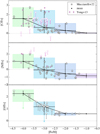 |
Fig. 1 [X/Fe] abundance ratios (where X = C, N, and O) of the low RGB stars of Mucciarelli et al. (2022, measurements: gray star symbols, upper limits: empty stars). Also shown are the mean values (dots connect by solid black lines) and the scatter (colored boxes) in 1-dex metallicity bins. Adding data from Yong et al. (2013, purple circles) for C and N increases the scatter, with the caveat that many points are actually upper limits (empty circles). |
2.1.3 Orbital parameters
Our stellar sample does not include any kinematic cut, so within the metallicity range covered by the observations (−4.5 ≤ [Fe/H] < −1.0 dex), we expect a mixture of stars with both in situ and accreted origin. To explore whether the origin of the abundance scatter is intrinsic or due to overlapping distributions of stars born in different environments, we study the dynamical properties of the stars in our sample.
It has been demonstrated that stars with common origin should remain clumped in the spaces defined by the integrals of motion (IoM, e.g., energy and angular momentum) even after they are completely phase-mixed within our Galaxy (Helmi & de Zeeuw 2000) and that chemistry plays a crucial role in complementing the complicated dynamical information (e.g., Matsuno et al. 2022; Horta et al. 2023; Ceccarelli et al. 2024). We thus exploited the extremely precise Gaia DR3 (Gaia Collaboration 2023) astrometry to get the 5D phase space information (i.e., position, proper motion, and parallax) for the stars in our sample. The spectroscopic line-of-sight velocities (Vlos) are taken from Norris et al. (2013) and Mucciarelli et al. (2022). To reconstruct each star’s orbit, we use the code AGAMA (Vasiliev 2019) assuming a McMillan (2017) potential for the MW. The orbits are integrated in a reference frame with the Sun positioned R⊙ = 8.122 kpc away from the Galactic Center (GRAVITY Collaboration 2018) and z⊙ = 20.8 pc above the Galactic plane (Bennett & Bovy 2019). The three components of the Solar velocity are set to (U⊙, V⊙, W⊙) = (12.9, 245.6, 7.78) km s−1 (Drimmel & Poggio 2018), as computed by joining the proper motion of Sgr A* (Reid & Brunthaler 2004) and the local standard of rest (Schönrich et al. 2010). To estimate uncertainties on the orbital parameters, we run 10 000 Monte Carlo simulations of the orbit for each star assuming Gaussian distributions for the uncertainties in the 6D phase space parameters. The uncertainties on the orbital parameters are defined as the 16th and 84th percentiles of their final distributions. The orbital parameters for the sample of unmixed halo stars adopted in this paper are listed in Table 2.
In Fig. 2, we present the distribution of the IoM of our sample stars, alongside the substructures identified in the stellar halo (Dodd et al. 2023). As a reference, we plot in gray the IoM of stars from the APOGEE sample, using the Gaia values listed in the APOGEE DR17 catalog (Abdurro’uf et al. 2022) to compute the orbits. Given the limited statistics of our stellar sample, we opted to associate the stars with a given substructure by looking directly at their position in the 3D IoM space (i.e., E, Lz, and L⊥). According to literature works based on clustering analyses on larger data sets (Ruiz-Lara et al. 2022; Dodd et al. 2023), we defined selection boxes in regions of the IoM spaces where different merging events are expected to have deposited their debris (see Fig. 2). Among all the targets analysed in this work, we find 14 stars tentatively associated with the Gaia–Sausage–Enceladus (GSE) merging event (pink box, Belokurov et al. 2018; Helmi et al. 2018), eight from the Sequoia dwarf galaxy (purple box, Myeong et al. 2019), two possibly related to Thamnos (yellow box, Koppelman et al. 2019), and finally four associated with the Helmi Streams (orange box, Helmi et al. 1999). We found no matching stars with the ED2, ED3, Antaeus, and Sagittarius substructures (Ibata et al. 1994; Oria et al. 2022; Dodd et al. 2023).
As shown in Fig. 3, the abundance ratios of different substructures tend to overlap in the [C/Fe], [N/Fe], [O/Fe], and [Mg/Fe] versus [Fe/H] diagrams1. No obvious nor distinct trends were observed, though there is marginal evidence that some Sequoia stars are among the most enhanced among all of the elements that exist. Larger samples are clearly required to derive a robust conclusion; still, with the data at hand we can hazard an interpretation of the spread in the elemental abundances as not due to the sum of distinct but tighter patterns, related to individual mergers. The observed scatter at these very low metallicities seems to be due to some intrinsic processes.
Orbital parameters (orbital energy, angular momentum along the z-axis, perpendicular component of the angular momentum, and line-of-sight velocity) with uncertainties for the unmixed halo stars.
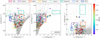 |
Fig. 2 Distribution of the sample stars color coded according to their [Fe/H] abundances in the IoM spaces. The circles are stars from Yong et al. (2013), and star symbols are stars from Mucciarelli et al. (2022). The APOGEE sample is plotted with filled gray points for reference. The boxes represent the positions occupied by previously identified substructures in the Galactic halo (Dodd et al. 2023). |
2.2 High-redshift systems
Recent JWST observations have captured rest-frame near-ultraviolet (UV) and optical spectra of distant galaxies exhibiting emission lines of C, N, and O from which accurate abundances relative to H have been determined (e.g., Arellano-Córdova et al. 2022; Schaerer et al. 2022; Heintz et al. 2023; Cameron et al. 2023). While most spectra obtained thus far closely resemble those of typical metal-poor star-forming galaxies in the local universe, a few luminous low-metallicity systems display anomalous super-solar C/O or N/O abundance ratios (e.g., Cameron et al. 2023; D’Eugenio et al. 2024; Marques-Chaves et al. 2024).
This has given rise to various speculations about the origin of such peculiar chemical features. It has been suggested that we might be witnessing the formation of proto-globular clusters, detecting the signatures of Wolf-Rayet or AGB stars that lose their outer layers through stellar winds, having a glimpse into early ISM pollution from Pop III and/or very massive stars (m★ ≥ 1000 M⊙) forming from collisions in dense clusters, or even seeing the effects of the activity of an active galactic nucleus (see Marques-Chaves et al. 2024, and references therein).
In Sect. 6, we develop GCE models tailored to reproduce the observed properties of the prototype extreme C- (GS-z12) and N-emitters (GN-z11), resting on our benchmark model for the MW. We compare the predicted abundances with CNO abundance estimates for GS-z12, GN-z11, and other similar systems (Bunker et al. 2023; Cameron et al. 2023; Isobe et al. 2023; Maiolino et al. 2024; D’Eugenio et al. 2024; Harikane et al. 2024; Ji et al. 2024; Senchyna et al. 2024; Xu et al. 2024).
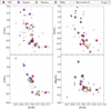 |
Fig. 3 [C/Fe], [N/Fe], [O/Fe], and [Mg/Fe] versus [Fe/H] abundances for our sample stars. The color code is the same as that for the boxes in Fig. 2. Unassociated stars are plotted in gray. |
3 Chemical evolution models
The increasing star-to-star scatter in chemical abundance ratios at low metallicity serves as a powerful tool to understand the earliest phases of the MW chemical enrichment (Argast et al. 2004; Cescutti et al. 2015; Wehmeyer et al. 2015; Griffith et al. 2023; Vanni et al. 2023). To gain insights into the early phases of CNO element evolution, we employ a GCE model that has been extensively tested against CNO abundance data of our and external galaxies (Romano etal. 2017,2019b,2020). Whilethemain focus of previous work was on [Fe/H] > −1.5 environments, here we add a detailed treatment of the first, inhomogeneous phases of galactic chemical enrichment (Sect. 4).
3.1 The Milky Way model
Hereafter, we provide an overview of the principal features, assumptions, and limitations of the adopted GCE model for the MW, which is constantly developed and improved. Further details are available in the quoted papers.
The model utilizes a multizone framework, dividing the Galactic disk into concentric annuli of 2 kpc each. It assumes that the in-situ inner halo and thick-disk components form from an initial phase of accretion of matter of primordial chemical composition (Chiappini et al. 1997, 2001). During the first ~3–4 Gyr of evolution (see Spitoni et al. 2019, 2021, for the calibration of the model against asteroseismic stellar ages), an efficient burst of star formation results in rapid gas depletion, leading to the formation of the most ancient stellar populations. The thin disk forms subsequently from a second, nearly independent infall event, on time scales ranging from ~3 Gyr for the inner disk up to a Hubble time for the outer regions (Romano et al. 2000; Chiappini et al. 2001). This ‘inside-out’ formation of the Galactic disk is required to reproduce the abundance gradients and the gas distribution along the disk (see Matteucci & Francois 1989, and references therein).
The star formation rate is described by the Schmidt-Kennicutt law (Kennicutt 1998), i.e., ψ(R, t) = v Lɡas(R, t)k. Here, the star formation rate is directly proportional to the gas surface density, Σgas, k is set equal to 1.5, and the star formation efficiency, v, is constant along the disk during the halo/thick-disk phase, while it becomes a function of the distance from the Galactic center during the thin disk formation (see Palla et al. 2020). The newly formed stellar mass is distributed in the mass range 0.1–100 M⊙ according to the Kroupa et al. (1993) IMF, characterizedbyaslopeof1.7inthehigh-mass regime.
3.2 Nucleosynthesis prescriptions
The chemical enrichment process is followed by tracking the evolution of all stable chemical species from hydrogen (H) to europium (Eu) and by considering the mass-dependent stellar evolutionary timescales (i.e., relaxing the instantaneous recycling approximation). This enables one to adequately follow the evolution of chemical elements that are produced on different timescales by stars of different initial mass and chemical composition.
For Pop II stars, we employed stellar yields dependent on the initial mass and metallicity of the stars that allowed a satisfactory fit to CNO abundance data for different MW components and early-type galaxies (Romano et al. 2019b, 2020, see also Romano et al. in prep). In particular, for low- and intermediate-mass stars (LIMS) with 1 ≤ m★/M⊙ ≤ 6, we retrieve the stellar yields for non-rotating stars from the FRUITY database (Cristallo et al. 2009, 2011, 2015). For massive stars (13 ≤ m★/M⊙ ≤ 120) that explode as CCSNe, we use the yields of Limongi & Chieffi (2018, their fiducial set R) computed for initial metallicities [Fe/H] = −3, −2, −1, and 0 and accounting for different rotational velocities (0, 150, and 300 km s−1). For type Ia SNe (SNela, exploding white dwarfs in binary systems), we assume the stellar yields of Iwamoto et al. (1999). SNIa primarily contribute to the bulk of iron production during later evolutionary stages and play a significant role in the decline of the [α/Fe] ratio at metallicities higher than investigated here. The nova outburst rate is incorporated following the methodology outlined in (Romano et al. 1999, 2021, and references therein). No contribution from novae is expected before 1 Gyr has elapsed from the beginning of star formation.
3.3 High-redshift galaxies: GN-z11 and GS-z12
As part of this study, we aim to reproduce the peculiar CNO abundances of a few young systems observed at high redshift. GN-z11 is a compact object with half-light radius ≤200 pc observed at z ≃ 10.6, hosting a ~109 M⊙ stellar population and characterized by a low-metallicity, N-rich ISM,  solar (Bunker et al. 2023; Cameron et al. 2023; Maiolino et al. 2024; Tacchella et al. 2023; Senchyna et al. 2024). Cameron et al. (2023) set a lower limit of log(C/O) > −0.78 to its carbon-to-oxygen ratio, yet we note that other extreme N-emitters found at high redshift have C/O ratios fairly similar to the ones of local metal-poor galaxies (Marques-Chaves et al. 2024; Schaerer et al. 2024). The galaxy GS-z12 (z ~ 12.5), with stellar and gaseous masses of ~5 × 10⁷ M⊙ and ~107 M⊙, respectively, and typical size of 100 pc has instead a carbon content unexpectedly high for its low metallicity, log(C/O) > −0.21 at log(O/H)+12 = 7.59 ± 0.25 (D’Eugenio et al. 2024).
To model these high-redshift galaxies, we run single-zone GCE models. Alike for the MW, fresh gas is accreted according to an exponentially decreasing law, dMinf /dt ∝ e−t/τ, where Minf is the total mass accreted and τ is the infall time scale. We assume that metal-free gas is quickly accreted (τ ~ 1–3 Myr) and efficiently converted into stars (v ~ 1–10 Gyr−1) within compact systems characterized by surface gas densities much higher than that of the MW (at the end of the simulation for GN-z11, the total surface mass density is Σ ≃ 7.5 × 10³ M⊙ pc−2, to be compared to values more than two orders of magnitude lower in the solar neighbourhood). The gas is converted into stars according to the Schmidt-Kennicutt law and the IMF is taken from Kroupa et al. (1993), similarly to what is done for the MW (see Sect. 3.1). The adopted nucleosynthesis prescriptions for Pop II stars are those described in Sect. 3.2. The free parameters of the model are fixed as to reproduce the observed properties of GN-z11 and GS-z12. Specifically, in the model for GN-z11 we assume the star formation history of Tacchella et al. (2023), namely, a low-level star formation episode (v = 1 Gyr−1) lasting 40 Myr, followed by a burst (v = 10 Gyr−1) of longer duration, 60 Myr, that forms most of the stellar mass of the system. This vigorous burst is fed by prominent infall of gas of primordial chemical composition that gives birth to a second generation of Pop III stars, overwhelming the contribution to the chemical enrichment from previous generations of Pop II stars (see Sect. 6.2). In the model for GS- z12, a shorter (10 Myr long) but similarly efficient (v ~ 10 Gyr−1) star formation burst is considered, resulting in a constant star formation rate of 1.6 M0 yr−1 and stellar mass at the time of the observations (350 Myr after the Big Bang) of log(M★/M⊙) = 7.60, in agreement with the values of  and log(M★/M⊙) = 7.68 ± 0.19 inferred by D’Eugenio et al. (2024). Finally, to match the low metallicity observed for GN-z11 in spite of its powerful starburst, we have to assume that a galactic outflow vents out more than a half of the stellar ejecta. This seems a reasonable request, since massive galactic outflows are actually known to be a key mechanism to regulate, or even quench, the star formation of high-redshift starbursts (e.g., Jones et al. 2019, and references therein). No galactic outflows are required for the smaller galaxy, GS-z12.
4 Model implementation
The role of Pop III stars is frequently overlooked in chemical evolution models. However, while at high metallicity ([Fe/H] > −1) stars are expected to form from a thoroughly mixed medium enriched by multiple stellar populations, which effectively washes out the distinctive chemical signatures of Pop III stars, at lower metallicities the contribution from the first massive stars becomes fundamental to explain the peculiar chemical abundances of ancient, metal-poor stars that survived to the present day (Koutsouridou et al. 2023; Vanni et al. 2023; Rossi et al. 2024). On the other hand, during the initial phases of galaxy evolution, stochastic processes associated with the star formation itself become crucial in shaping the evolution and chemical enrichment history of galaxies (e.g., Caplar & Tacchella 2019; Tacchella et al. 2020; Wang et al. 2022; Pallottini & Ferrara 2023; Iyer et al. 2024).
To model the early chemical enrichment phases of our Galaxy we implement the GCE model described in Sect. 3 in order to account for a pre-enrichment driven by Pop III stars and a stochastic star formation process. We assume that in the initial phases of formation, the MW is built up by gas clumps with different gas densities that merge into the MW main branch. We assume that a single Pop III SN precursor is formed in each clump, with properties (mass, internal mixing level, and explosion energy) randomly selected from the Heger & Woosley (2010) model grid. The mass of Pop III stars is stochastically selected within the mass range 10 ≤ mPop III/M⊙ ≤ 100, while the explosion energy, ESN, is assigned by randomly choosing among four different types of SNe, each with a specific energy range: faint (E512= 0.3–0.6 erg), core-collapse (E51 = 1.21.5 erg), high-energy (E51 = 1.8–3.0 erg), and hypernovae (E51 = 5.0–10 erg). We have not included the pre-enrichment from PISNe in our analysis. In fact PISNe, with initial masses ranging from 140 to 260 M0, are predicted to enrich the surrounding ISM up to [Fe/H] ≈ −2 while underproducing N, [N/Fe] < −2 (Salvadori et al. 2019), and no stars with such low N abundances are present in our sample (see Sect. 2). The clumps are assumed to be characterized by different dilution factors (101,102,103, and 104 ; see also Nandal et al. 2024a,b), defined as the ratio between the hydrogen mass and the mass ejected by Pop III SNe. This factor regulates how much the SN ejecta is diluted by the pristine surrounding medium and is a free parameter of our model. We note that assuming different dilution factors is equivalent to consider clumps of different sizes/densities. Finally, for each dilution factor, we consider 200 realisations of the chemical enrichment.
After the explosion of Pop III SNe, the metallicity of the gas in each clump reaches a level that triggers the formation of Pop II stars. We then track the subsequent chemical evolution assuming the yields of Limongi & Chieffi (2018) for massive stars in the case of fast rotators with vrot = 150 km s−1 and the FRUITY yields for LIMS (see Sect. 3.2).
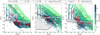 |
Fig. 4 [C/Fe] (left), [N/Fe] (middle), and [O/Fe] (right) versus [Fe/H] abundances predicted by our stochastic chemical evolution model for the Galactic halo (squares). Different shades of green represent different dilution factors (see text and Nandal et al. 2024a,b). Red stars, purple circles, and brown triangles respectively represent the data sets of Mucciarelli et al. (2022), Yong et al. (2013), and Amarsi et al. (2019). Empty symbols represent upper limits. The continuous curves in shades of gray represent the predictions of the homogeneous GCE model without pre-enrichment from Pop III stars, assuming the yield sets of Limongi & Chieffi (2018) with different rotation velocities for massive stars. |
5 Early chemical enrichment: Exploiting long-lived stars in the Milky Way
In this section we present the results of chemical evolution models for the MW. In Fig. 4, we show the predicted abundance ratios of CNO elements as a function of [Fe/H] compared with observational data (Mucciarelli et al. 2022; Yong et al. 2013; Amarsi et al. 2019). Different shades of green represent the predictions of the stochastic GCE model obtained assuming different dilution factors for the Pop III star ejecta, i.e., different sizes/densities for the star-forming clumps at the beginning of the simulation (see Sect. 4). The first thing to note is that, to reproduce the full range of [Fe/H] values covered by our stellar sample (Sect. 2.1), we need to account for different dilution factors3 ranging from 101 to 104 . Specifically, the higher dilution factors allowed us to reproduce the bulk of the observational data at [Fe/H] < −2. In this case, the ejecta from the first SNe are dispersed in denser (or larger) gas knots that contain higher amounts of neutral hydrogen, resulting in a shift of [Fe/H] toward the low metallicity regime. As the dilution factor decreases, the iron released by Pop III SNe is diluted in a less dense environment, meaning the stellar clump is less compact, or in a smaller bubble, resulting in an increase in [Fe/H] abundance. We note that our assumptions on the dilution factors only affect the [Fe/H] abundances, which depend on the total amount of neutral hydrogen present in the stellar clumps, while the [X/Fe] ratios remain independent from these assumptions.
As shown in Fig. 4, our stochastic GCE model successfully reproduces the scatter observed at low metallicity for both C, N, and O, even if it is worth noting that for [Fe/H] < −2.5 we could only set upper limits to the O abundances. In Fig. 4, we also compare our results with the predictions of homogeneous GCE models that do not incorporate pre-enrichment from Pop III stars. The homogeneous GCE models adopt yields for Pop II massive stars from Limongi & Chieffi (2018), computed with different initial rotational velocities (vrot = 0, 150, and 300 km s−1) and metallicities ([Fe/H] = −3, −2, −1, and 0) of the stars. Notice that for [Fe/H] < −3, we use the yield set corresponding to the lowest [Fe/H] value. It is clearly seen that, regardless of the assumed rotation velocities, homogeneous models fail to reproduce the observed [X/Fe] abundance ratios at [Fe/H] < −2.5. This is particularly evident for C and N and it is, at least partly, due to the fact that the yield grid of Limongi & Chieffi (2018) does not include Z = 0 stellar models. Indeed, at higher metallicities ([Fe/H] > −2.5) the models reach a satisfactory agreement with the observations. There is a clear tendency to overproduce C, though. Regarding the [N/Fe] abundance ratio, we notice that models assuming massive star yields computed with different rotational velocities adequately represent stars with low N abundances ([N/Fe] < 0) across the full metallicity range. Nevertheless, even when assuming fast rotation, which boosts primary N production at low metallici- ties (Meynet et al. 2006; Limongi & Chieffi 2018), these models fall short of reproducing N-enriched stars.
Having calibrated our stochastic GCE model to reproduce the dispersion of our data sample through an appropriate choice of the dilution factors, we now delve into the nature of the polluters responsible for the variation of chemical abundance ratios within our stellar sample at low metallicity.
In Figs. 5–9, we present ‘chemical density maps’ for the present-day stellar population in the MW halo, as predicted by our model. In all figures, different panels refer to different explosion energies of Pop III SNe contributing to the initial phases of chemical enrichment. As is evident from the figures, different Pop III SN types contribute differently to the observed scatter. Low-energy Pop III SNe (faint and CCSNe) are responsible for high values of [C/Fe] > 1, [N/Fe] > 0.5, and [O/Fe] > 1.5 and struggle to accurately reproduce the regions with [C/Fe] < 0.5, [N/Fe] < 0, and [O/Fe] < 1. As the explosion energy of Pop III SNe increases (high-energy SNe and hypernovae), the [C/Fe] < 0.5 and [O/Fe] < 1 data points are well reproduced. In contrast, despite accounting for the influence of energetic Pop III SNe, regions at [N/Fe] < −0.5 are sparsely recovered. This discrepancy does not necessarily indicate an issue, but rather suggests that the predominant polluters responsible for enriching these stars could be Pop II stars with diverse rotation velocities. At this point, it is essential to clarify that our study does not aim to identify the potential descendants of the first stars. Although our results seem indeed to suggest that among carbon-, nitrogen-, and oxygen-enhanced stars there may be possible candidates, it is beyond the scope of this work to engage in such speculation. The main goal of this paper is to shed light onto the early evolution of our own and other galaxies, accounting for the contribution of all possible stellar polluters acting at early times.
In the light of the comparison of our results for the MW with what can be observed at high redshift, it is important to discuss the density maps for log(N/O) and log(C/O) versus log(O/H) + 12. These are presented in Figs. 8 and 9, although the presence of many upper/lower limits in our stellar sample prevented us from drawing definitive conclusions. As it is evident from the figures, our predictions cover a broad range in metallic- ity, 7 < log(O/H) + 12 < 9.5. Notably, there is a clear trend in the abundance of log(N/O) and log(C/O) with varying energy levels of Pop III SNe. With pre-enrichment from faint SNe, it is possible to achieve extremely high values of log(N/O) up to ≈ −0.5 and log(C/O) up to 0.5 . As the energy of Pop III SNe increases, regions with log(N/O) > −1 and log(C/O) > 0 become less populated, while regions with −2.5 < log(N/O) < −1 and −1 < log(C/O) < 0 at 7.5 < log(O/H) < 9.5 start to fill, reflecting the influence of core-collapse and high-energy SNe. Finally, with hypernovae, areas with higher metallicity, log(O/H) > 8.5, and low values of log(N/O) < −2.5 and log(C/O) < −1 are well reproduced. It is important to highlight the effects of the two extreme Pop III SN energetic regimes: only faint SNe manage to populate the regions with log(N/O) > −1 and log(C/O) > 0, while hypernovae primarily impact regions with log(N/O) < −2.5 and log(C/O) < −1.
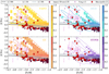 |
Fig. 5 Predicted density maps of [C/Fe] versus [Fe/H] for stellar populations inhabiting the MW halo. The different panels and colors highlight the contributions of various Pop III SN types: faint, core-collapse, high-energy, and hypernovae. The gray continuous lines represent the predictions of the homogeneous model without the contribution of Pop III SNe, for different rotation velocities of Pop II massive stars (vrot = 0, 150, and 300 km s−1, Limongi & Chieffi 2018). Data (symbols, see figure legend) are from Mucciarelli et al. (2022), Yong et al. (2013), and Amarsi et al. (2019). Empty symbols represent upper limits. |
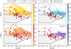 |
Fig. 6 Same as Fig. 5 but in the [N/Fe]–[Fe/H] space. Nitrogen abundances for the unmixed RGB stars of Mucciarelli et al. (2022) have been derived as described in Sect. 2.1.1. |
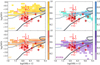 |
Fig. 8 Same as Fig. 6 but in the log(N/O)- log(O/H) + 12 space. Nitrogen and oxygen abundances for the unmixed RGB stars of Mucciarelli et al. (2022) have been derived as described in Sect. 2.1.1. |
6 Early chemical enrichment: The gaseous medium of high-redshift galaxies
Recent JWST spectroscopy of high-redshift, metal-poor galaxies, particularly the most luminous ones, such as GN-z11 (Oesch et al. 2016) and CEERS-1019 (Finkelstein et al. 2017), has revealed gas substantially enriched in nitrogen (see Bunker et al. 2023; Cameron et al. 2023; Maiolino et al. 2024; Marques- Chaves et al. 2024; Senchyna et al. 2024), sparking renewed interest in the evolution of the CNO elements and prompting new inquiries into their origins. While N-emitters tend to have normal C content for their metallicities (see Schaerer et al. 2024, their figure 2), extreme C enhancement is found in a few systems (D’Eugenio et al. 2024), which deserves special attention.
In this section we aim to provide testable predictions for a MW- like galaxy observed at different redshifts, along with a possible interpretation of the high N/O (C/O) ratio measured for GN-z11 (GS-z12), within the framework of our GCE model, including pre-enrichment by Pop III SNe with yields dependent on the mass, internal mixing level, and explosion energy of the progenitor star (Heger & Woosley 2010).
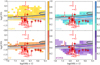 |
Fig. 9 Same as previous figure but for carbon. Carbon and oxygen abundances for the unmixed RGB stars of Mucciarelli et al. (2022) have been derived as described in Sect. 2.1.1. |
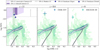 |
Fig. 10 Theoretical log(N/O) versus log(O/H)+12 for a proto-MW galaxy seen at different redshifts. Density maps and contours refer to the predictions of the stochastic GCE model, while the solid lines refer to the predictions of the homogeneous GCE model. Abundances measured in GN-z11 (z = 11, Bunker et al. 2023; Cameron et al. 2023; Senchyna et al. 2024), CEERS-1019 (z = 8.6, Marques-Chaves et al. 2024), and RXCJ2248-ID (z = 6, Topping et al. 2024) are also shown for comparison (symbols and shaded areas). |
6.1 Milky Way counterparts at high redshift
In Fig. 10, we display density maps in the plane log(N/O)- log(O/H) + 12 for a MW-like galaxy4 seen at various redshifts. After the initial chemical enrichment by Pop III SNe, which sets a wide range of initial abundances in log(O/H) and log(N/O), there is a phase of rapid chemical enrichment. The density contours show that most of the clumps that are in the process of merging to form the halo, reach values of log(N/O)−1 and log(O/H) + 12 ~ 8.5 after only ~400 Myr (z ~ 11). Observations of a MW-like galaxy at high redshift would not resolve the different knots and would thus measure those average values, which also agree with the predictions of homogeneous GCE models including massive fast rotators. The subsequent evolution proceeds slowly. Over the approximately 500 million years elapsed between z ~ 11 and z ~ 6, the average metallic- ity gradually increases. At z ~ 6, the gas reaches log(O/H) ≈ 9 and log(N/O) ≈ −0.7, reflecting the ongoing enrichment processes and contributions from subsequent stellar generations. In Appendix A we display our predictions for a proto-MW up to z ~ 2 and provide the maps also for the C/O and C/N abundance ratios.
Figure 10 also shows the log(N/O) values measured in GN- z11 at z = 10.6 (Bunker et al. 2023; Cameron et al. 2023; Maiolino et al. 2024; Senchyna et al. 2024), in CEERS-1019 at z = 8.6 (Marques-Chaves et al. 2024) and in RXCJ2248-ID at z ~ 6 (Topping et al. 2024). Note that while our predictions for the proto-MW successfully cover the observed metallicity range of 7 < log(O/H) + 12 < 9, they struggle to reproduce the high observed values of log(N/O) > –0.5. This discrepancy is not unexpected: these systems are significantly brighter and more massive than what is expected for the MW progenitor at the same redshifts. For instance, at z ≈ 11, the surface stellar density predicted for a proto-MW is Σ* ~ 430 MΘ pc–2, whereas for GN- z11, it is approximately four times higher, Σ* ~ 1650 MΘ pc–2 (Tacchella et al. 2023). On the other hand, our results indicate that it is possible to achieve values as high as log(N/O) > −0.5 in some regions of a forming MW analog within the metallic- ity range of 7.5 < log(O/H) + 12 < 8.0. As already discussed in Sect. 5, such high N/O values are due to the contribution of faint Pop III SNe (see Fig. 8). Accounting for the effects of stellar rotation in Z = 0 massive star models would likely lead to even higher N/O ratios (Meynet et al. 2006; Limongi & Chieffi 2018), but these are not implemented in the yields of Heger & Woosley (2010) for Pop III stars adopted in this work.
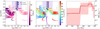 |
Fig. 11 Chemical enrichment of GN-z11. Left and middle panels: predicted log(N/O) versus log(O/H)+12 for GN-z11. Different evolutionary tracks represent different Pop III star-forming clumps, which merge into the main branch of the galaxy. The tracks are color coded according to time elapsed since the beginning of star formation (left) and stellar mass (middle). The light purple trapezoid, the dark purple rectangle, and the gray stripe represent the conservative and fiducial results for the abundances of GN-z11 by Cameron et al. (2023). The blue points are the photoionization modeling results for GN-z11 by Senchyna et al. (2024). Right panel: star formation history of GN-z11 according to Tacchella et al. (2023, red line and shaded area) and as adopted in the model (gray line). |
6.2 Extreme abundance ratios at high redshift
In this section we deal with compact metal-poor, high-redshift systems that display C/O or N/O abundance ratios at variance with what is expected for their metallicities.
6.2.1 GN-z11
Figure 11 presents the elemental abundance ratio log(N/O) as a function of log(O/H) + 12 as a proxy for metallicity in the ISM of GN-z11, predicted by a model tailored to this galaxy (see Sect. 3.3). The different traces illustrate the chemical evolution of different clumps, each harboring one Pop III polluter at the beginning of the simulation, at fixed density so as to reproduce the observed properties of GN-z11. In the left panel, the traces are color coded based on the time elapsed from the beginning of star formation in the model, whereas in the middle panel different colors indicate different masses of the Pop III stars that pre-enriched the ISM. We note that we specifically selected models where the ISM was pre-enriched by faint Pop III SNe, as Pop III SNe with higher explosion energies are not able to achieve log(N/O) values that align with the observational data (see Fig. 8). The stellar mass and star formation rate (Fig. 11, right-hand panel) predicted by the model at the time of the observations, 440 Myr after the Big Bang, are 8.8 × 10⁸ MΘ and 25 M⊙ yr–1, respectively, which perfectly align with the data (by construction).
Two distinct sets of evolutionary tracks are visible, each corresponding to different star formation bursts. The dark purple tracks in Fig. 11 (left panel) represent the chemical evolution during the initial low-level star formation activity, which lasts for approximately 40 Myr from the onset of galaxy formation. The lighter colored tracks correspond to the second star formation burst, which begins 40 Myr after the beginning of the simulation and evolves for approximately 60 Myr. Both bursts are fed by infall of gas of primordial chemical composition and initiated by pre-enrichment from Pop III stars, which establishes the starting points of the log(N/O) versus log(O/H) + 12 tracks.
In the first star formation episode, we observe three distinct chemical enrichment paths, each directly linked to the mass of the Pop III SN that pre-enriched the ISM. In the first path, the trace starts at low values of log(N/O) < −1 and log(O/H) + 12 < 6.0, gradually increasing in log(N/O) over time. The starting point of the track reflects the enrichment from low-mass Pop III stars (mPopIII< 40 MΘ), as shown in the middle panel of Fig. 11, while the subsequent increase in log(N/O) and slight decrease in log(O/H) + 12 is due at first to the continuous infall of pristine gas and then to the overwhelming contribution of massive Pop II stars. The second path involves Pop III SNe with masses in the range 40−80 MΘ that pre-enrich the ISM to log(O/H) + 12 < 7.0, and log(N/O) > -1.5 values. Following this initial phase, the log(N/O) ratio rapidly declines due to significant oxygen production from subsequent Pop II SNe, to slightly increase later mostly because of primary nitrogen production from Pop II massive stars boosted by rotation. Finally, the third path begins with pre-enrichment from massive Pop III SNe (mPopIII > 80 MΘ), resulting in high log(N/O) ~ – 1 values and 7.0 < log(O/H) + 12 < 7.5. This path shows an initial decreasing trend in metallicity (with an approximately constant log(N/O) value), followed by a subsequent increase. The initial decline in log(O/H) is attributed to the dilution due to the infall of pristine gas, followed by a chemical enrichment path similar to the one of the previous scenario, predominantly driven by the contribution of successive generations of Pop II stars.
As the second burst begins, fueled by the infall of gas of primordial chemical composition, a second episode of pre-enrichment by Pop III stars occurs that together with the cumulative enrichment from the first burst establishes the starting point of the new evolutive track. Following this initial phase, the chemical evolution is predominantly driven by Pop II star formation, dominating the later stages of evolution. This path shows an initial decreasing trend in metallicity with an approximately constant log(N/O) value. The initial decline in log(O/H) is attributed to the dilution due to the infall of pristine gas, followed by chemical enrichment predominantly driven by the contribution of successive generations of Pop II stars.
The log(N/O) values predicted by our GCE model intercept the value observed in GN-z11 within the uncertainties after 100 Myr from the beginning of galaxy formation. Setting the start of star formation at 340 Myr after the Big Bang in the model makes the predicted abundance to agree with the observed one at z ≃ 10.6. This suggests that the extreme N-enhancement observed at high redshift can be obtained by accounting for a pre-enrichment of the ISM from massive Pop III stars with mPop III ≥ 50–85 M⊙ ending their lives as faint SNe. Notably, at the epoch of the observations the predicted star formation rate is 26 M⊙ yr–1, in agreement with the observed value,  M⊙ yr–1, and the average stellar age is 20 Myr, which is comparable to the estimated value of
  Myr (Tacchella et al. 2023).
In conclusion, we propose an alternative scenario to explain the high log(N/O) ratio observed in GN-z11 and other high- redshift extreme N-emitters. Specifically, we suggest that these galaxies experienced an enrichment from massive, faint Pop III SNe, which could account for the elevated nitrogen levels. This scenario provides a compelling explanation for the chemical signatures detected in such early galaxies.
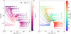 |
Fig. 12 Predicted log(C/O) versus log(O/H) + 12 for GS-z12. The evolutionary tracks represent different PopIII star-forming clumps that merge into the main branch of the galaxy. The tracks are color coded to indicate the time elapsed since the beginning of star formation (left panel) and the PopIII stellar mass (right panel). Also shown is the measured log(C/O) abundance for GS-z12 as derived by D’Eugenio et al. (2024). The blue marker represents the estimate obtained through a Bayesian modeling of the spectrum, while the gray stripe marks the lower limit derived using the photoionization models of Gutkin et al. (2016). |
6.2.2 GS-z12
Figure 12 shows the elemental abundance ratio log(C/O) as a function of log(O/H) + 12 in the ISM of GS-z12, based on predictions from a model specifically designed for this galaxy. In the case of GS-z12, a single star formation burst is considered (see Sect. 3.3). The evolutionary tracks are color coded similarly to those in Fig. 11, with the colors indicating either the time elapsed since the onset of star formation (Fig. 11, left panel) or the stellar mass of the Pop III progenitors (Fig. 11, right panel). Similar to what is found for GN-z11, distinct evolutionary tracks are clearly visible, primarily shaped by the masses of the Pop III stars that pre-enrich the ISM.
Three sets of evolutionary tracks can be recognized. In the first set, the tracks start at low values of log(C/O) ≈ –0.5 and log(O/H) + 12 < 6.5, showing a steady decrease of log(C/O) as time progresses. This initial phase is driven by enrichment from low-mass Pop III stars (mPop:III < 20 MΘ) that produce significant amounts of carbon with minimal oxygen contribution. As Pop II stars enter the scene, log(C/O) decreases while the oxygen abundance increases, reflecting the dominant contribution of Pop II SNe during later evolutionary phases.
The second set of tracks involves a pre-enrichment by Pop III stars with masses between 40 and 60 M⊙. These stars enrich the ISM to high metallicities, log(O/H) + 12 ~ 8.5, and –0.2 ≲ log(C/O) < 0.1. The metallicity initially decreases, while log(C/O) remains constant, due to the contribution of the primordial infalling gas, which dilutes the metals without affecting their abundance ratio. Subsequently, log(C/O) decreases due to the contribution to the enrichment by massive Pop II SNe.
The third path corresponds to Pop III stars with masses between 60 and 80 M⊙ . These massive stars pre-enrich the ISM to low metallicities, log(O/H) + 12 ≲ 7.5, while log(C/O) reaches high values, exceeding 0.25 dex. After an initial phase in which the infall of pristine gas dilutes all the metals in the same way, the ISM becomes enriched in oxygen from Pop II SNe and the log(C/O) ratio begins to decrease, while log(O/H) + 12 steadily increases.
The fourth evolutionary path is initiated by the most massive Pop III stars (mPop:III > 80 MΘ), leading to initial log(C/O) ≲ –0.4 and high metallicity, log(O/H) – 8.5. As the track progresses, there is a decrease in log(O/H) + 12, again due to dilution from infalling pristine gas, followed by an enrichment phase dominated by Pop II stars, which gradually increases the oxygen abundance. The log(C/O) values remain relatively stable, reflecting the fact that the most massive Pop III stars exploding as faint SNe are characterizes by C/O ratios in their ejecta that resemble those of Pop II CCSNe (see Fig. 9).
Our inhomogeneous model predicts log(C/O) values that match the one observed in the ISM of GS-z12 after a 10-Myr long star formation burst. At the time of observation, the predicted star formation rate is approximately 1.6 MΘyr–1, in good agreement with the observed one. The average stellar age is ~10 Myr and the stellar mass is log(M*/MΘ) = 7.60, which also agrees with the observational estimate.
In conclusion, the elevated log(C/O) ratio of GS-z12 can be attributed to early carbon production by Pop III stars of masses 50–70 M⊙, followed by later oxygen enrichment from Pop II stars.
7 Discussion
7.1 Milky Way galaxy
The contribution of Pop III stars is often neglected, or considered negligible, in chemical evolution studies of the MW. For instance, Ballero et al. (2006), using the yields of Woosley & Weaver (1995) for Pop II SNe and those of Heger & Woosley (2002) for PISNe, conclude that the effects of Pop III stars on the Galactic evolution of CNO elements are negligible, if only one or two generations of such stars are formed.
In our study, there are two significant differences compared to Ballero et al. (2006) that lead to different conclusions. First, in this work we consider the contribution of Pop III SNe with a wide range of explosion energies, from low-energy, faint SNe to highly energetic hypernovae (Heger & Woosley 2010), which results in theoretical [X/Fe] abundance ratios covering a broader spectrum. Second, we include a stochastic star formation component that is fundamental to adequately describe the initial phases of galaxy formation (see Rossi et al. 2021). This approach avoids using IMF-averaged yields and instead considers the contributions of individual Pop III SNe during the early stages of the MW evolution. Averaging the yields over the IMF tends to smooth out the unique chemical signatures of individual Pop III SNe, resulting in predicted [X/Fe] ratios that are systematically lower (or higher) than the most extreme values.
By incorporating these factors, our approach reevaluates the significant role that Pop III SNe could play when their varied explosion energies and stochastic formation processes are taken into account.
Our findings are consistent with those of other recent studies. For example, Vanni et al. (2023), utilizing a general parametric model for early metal enrichment, illustrate how the star-to- star scatter in abundance ratios among low-metallicity halo stars is influenced by the different initial masses and SN explosion energies of Pop III SNe. Conversely, at higher metallicities, the dispersion in abundance ratios decreases with the increased contribution from typical Pop II stars. Similarly, Koutsouridou et al. (2023), employing a cosmological chemical evolution model for the MW, emphasize the necessity of incorporating faint Pop III SNe to accurately reproduce the carbon-enriched stars at [Fe/H] < –2 (see also Rossi et al. 2023).
The scenario proposed in this work is not intended to be exclusive. We do not exclude the possibility that other sources with different properties may have contributed to the chemical enrichment of the Galaxy at low metallicities. For instance, Chiappini et al. (2005) investigated the impact of stars with metallicities Z = 10–8 and a wide range of initial rotational velocities (Hirschi et al. 2004) on the early MW chemical evolution. Their study concluded that scenarios involving fast rotators at low metallicities are necessary to explain the observed high N abundances in halo stars. Our aim with our findings is to complement the existing research.
7.2 C- and N-enhanced high-redshift systems
Different scenarios have been proposed to explain the extreme N/O abundance ratios measured in high-redshift systems, such as GN-z11 and CEERS-1019 (Cameron et al. 2023; Marques- Chaves et al. 2024). Kobayashi & Ferrara (2024) proposed a dual-burst model emphasizing the crucial role of Wolf-Rayet (WR) stars as N producers during the secondary burst phase. Prantzos et al. (2017) and Gratton et al. (2019) linked chemical peculiarities in globular clusters to the extreme patterns observed in galaxies like GN-z11. On the same line, D’Antona et al. (2023) proposed that the high N content of GN-z11 could be due to the formation of second-generation stars from pristine gas and asymptotic giant branch stellar ejecta in a massive proto-globular cluster. Charbonnel et al. (2023) and Nagele & Umeda (2023) explored the impact of metal-enriched stars, especially those within the mass range 103–105 M⊙, on early galaxy chemistry. Isobe et al. (2023) investigated chemical abundances in 70 galaxies, correlating them with WR stars, supermassive stars (SMS), and tidal disruption events.
At the same time, various studies have analysed different efficient N production channels in stars. For instance, Meynet et al. (2006) and Choplin (2018) delved into the effects of rapid rotation on massive stars, while Heger & Woosley (2002) and Takahashi et al. (2018) explored PISNe. Nandal et al. (2024a) investigate the impact of primordial SMS with masses in the range 500-9000 Mθ and Vink (2023) highlights the potential of very massive stars (100–1000 M⊙) as efficient N polluters. Marques-Chaves et al. (2024) consider the contribution of both WR stars and SMS with masses over 1000 M⊙. Finally, Nandal et al. (2024b) emphasize the unique contribution of Pop III and extremely metal-poor stars in enhancing nitrogen abundance in high-redshift galaxies, considering different rotation velocities for stars in the mass range 9-120 M⊙.
While a comprehensive interpretation remains elusive, our study contributes to the intricacies of this complex scenario, providing an alternative perspective on high-redshift N-emitters. Utilizing our stochastic GCE model benchmarked against MW data first and, then, tailored to GN-z11, we demonstrate that it is possible to achieve log(N/O) > –0.5 through enrichment mechanisms involving low-energy (ESN ≤ 0.6 × 1051), faint SNe with masses exceeding 50 Mθ . While these pristine stars are expected to be rare, their contribution to the chemical enrichment within metal-poor environments could become relevant, should the galaxy-wide stellar IMF (gwIMF) be shifted toward higher masses (Rossi et al. 2021; Koutsouridou et al. 2024). Indeed, evidence of a top-heavy IMF in starbursts has accumulated over the years (e.g., Jerábková et al. 2018; Schneider et al. 2018; Zhang et al. 2018; Zinnkann et al. 2024), making our findings particularly intriguing.
As for the class of the rarer extreme C-emitters (see Schaerer et al. 2024, their figure 2), we study the emblematic case of GS- z12. Also in this case, massive Pop III stars that explode as faint SNe are found to play a key role in reproducing the observed high C/O ratio at low metallicity, notwithstanding the lowest stellar mass reached by GS-z12.
8 Conclusions
To explore the earliest phases of chemical enrichment in galaxies, we have implemented a stochastic star formation component and detailed Pop III nucleosynthesis prescriptions in a GCE model that already satisfactorily reproduces the main observed properties of the Galaxy (see Sects. 3.1 and 4). By first comparing our model predictions with a homogeneous stellar sample of unmixed stars (Sect. 2.1.1) whose chemical abundances reflect the composition of their natal birth clouds, we demonstrated that the scatter in CNO abundances and abundance ratios observed in the MW halo can be largely attributed to the contributions of Pop III SNe with different masses and explosion energies. We then extended the model to the high-redshift universe and predicted the chemical abundance ratios for a proto-MW galaxy seen at different redshifts (Sect. 6.1). Finally, we adapted the model and provided an alternative interpretation of the chemical abundances observed in GN-z11 and GS-z12 (Sect. 6.2). Our key findings can be summarized as follows:
- (i)
The spread in chemical abundances (C, N, O, and Mg) of our stellar sample is not related to the sum of distinct, tighter patterns due to the accretion of different substructures in individual mergers. At the low metallicities covered by our sample, the observed scatter is likely due to intrinsic processes;
- (ii)
To reproduce the observed spread in C and N, it is necessary to consider stochastic chemical enrichment driven by Pop III stars of different masses and explosion energies, ranging from low-energy faint SNe to hypernovae. Specifically, low- energy Pop III SNe (faint and CCSNe) have an impact on the dispersion at [C /Fe] > 1 and [N/Fe] > 0, whereas energetic Pop III SNe contribute at [C/Fe] < 0.5 and [N/Fe] < 0 and higher [Fe/H] values;
- (iii)
High log(N/O) > –1 are predicted to be observed in MW halo stars, primarily driven by chemical enrichment from faint Pop III SNe, which are the only kind of Pop III SNe (at least, when adopting the yields of Heger & Woosley 2010) capable of achieving such high N enrichment levels;
- (iv)
The chemical enrichment of MW-like galaxies is predicted to be very rapid at high redshift (z ∼ 11) and followed by a more gradual enrichment at later stages (z ∼ 2; see Appendix A). We anticipate a large scatter in CNO abundance ratios: –2 < log(N/O) < –0.2, –1.5 < log(C/O) < 0.2, and 0 < log(C/N) < 1.7 (see Fig. A.1);
- (v)
We propose an alternative interpretation of the extremely high N abundance measured in the low-metallicity compact system GN-z11. Namely, we propose that before being observed, the galaxy was chemically enriched by massive faint Pop III SNe, resulting in log(N/O) > –0.25;
- (vi)
Pre-enrichment by faint Pop III SNe could also be the key to explaining the high C/O ratios observed in young low- metallicity systems, such as GS-z12.
In conclusion, this study has highlighted the importance of the contribution of Pop III stars to the early phases of galactic evolution. Our results emphasize the complexity of chemical enrichment processes in the early stages of galaxy formation and underscore the need for further efforts to better understand the contribution of Pop III stars. Future work should integrate more detailed observational data and more sophisticated theoretical models to reduce the remaining uncertainties and provide a clearer picture of chemical enrichment mechanisms in the primordial universe. In this respect, the full exploitation of the capabilities of space telescopes such as JWST and Euclid will be crucial.
Data availability
Full Tables 1 and 2 are available at the CDS via anonymous ftp to cdsarc.cds.unistra.fr (130.79.128.5) or via https://cdsarc.cds.unistra.fr/viz-bin/cat/J/A+A/691/A284
Acknowledgements
We thank Piercarlo Bonifacio and Elisabetta Caffau for providing useful suggestions and commenting on an earlier version of this paper. This research is part of the project “An in-depth theoretical study of CNO element evolution in galaxies” that is supported by the Italian National Institute for Astrophysics (INAF) through Finanziamento della Ricerca Fondamentale, Theory Grant Fu. Ob. 1.05.12.06.08 (PI: D. Romano). DR and AM acknowledge financial support from PRIN-MIUR-22, project “LEGO – Reconstructing the building blocks of the Galaxy by chemical tagging” (P.I. A. Mucciarelli). Based on observations collected at the ESO-VLT under programmes 68.D-0546, 69.D- 0065, 70.D-0009, 71.B-0529, 072.B0585, 074.B-0639, 076.D-0451, 078.B-0238, 090.B-0605, 092.D-0742, 099.D-0287, 0103.D-0310, 0104.B-0487, 0104.D- 0059, 165.N-0276, 169.D-0473, 170.D-0010, 281.D-5015, and 380.D-0040, at the La Silla Observatory under the programme 60.A-9700, at the Magellan telescope under programmes CN2017A-33 and CN2017B-54, and on data available in the ELODIE archive. This work has made use of data from the European Space Agency (ESA) mission Gaia (https://www.cosmos.esa.int/gaia), processed by the Gaia Data Processing and Analysis Consortium (DPAC, https://www.cosmos.esa.int/web/gaia/dpac/consortium). Funding for the DPAC has been provided by national institutions, in particular the institutions participating in the Gaia Multilateral Agreement. This work made use of SDSS-IV data. Funding for the Sloan Digital Sky Survey IV has been provided by the Alfred P. Sloan Foundation, the U.S. Department of Energy Office of Science, and the Participating Institutions. SDSS-IV acknowledges support and resources from the Center for High Performance Computing at the University of Utah. The SDSS website is www.sdss4.org. SDSS-IV is managed by the Astrophysical Research Consortium for the Participating Institutions of the SDSS Collaboration including the Brazilian Participation Group, the Carnegie Institution for Science, Carnegie Mellon University, Center for Astrophysics | Harvard & Smithsonian, the Chilean Participation Group, the French Participation Group, Instituto de Astrofísica de Canarias, The Johns Hopkins University, Kavli Institute for the Physics and Mathematics of the Universe (IPMU) / University of Tokyo, the Korean Participation Group, Lawrence Berkeley National Laboratory, Leibniz Institut für Astrophysik Potsdam (AIP), Max-Planck-Institut für Astronomie (MPIA Heidelberg), Max-Planck-Institut für Astrophysik (MPA Garching), Max-Planck-Institut für Extraterrestrische Physik (MPE), National Astronomical Observatories of China, New Mexico State University, New York University, University of Notre Dame, Observatário Nacional / MCTI, The Ohio State University, Pennsylvania State University, Shanghai Astronomical Observatory, United Kingdom Participation Group, Universidad Nacional Autónoma de México, University of Arizona, University of Colorado Boulder, University of Oxford, University of Portsmouth, University of Utah, University of Virginia, University of Washington, University of Wisconsin, Vanderbilt University, and Yale University.
Appendix A Predictions for Milky Way analogs at different redshifts
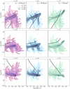 |
Fig. A.1 Chemical density maps for MW analogs seen at different redshifts. The predictions of the classic, homogeneous GCE model (solid lines; see text) are also shown. |
In Fig. A.1 we display the density maps in different planes, log(N/O), log(C/O), and log(C/N) versus log(O/H) + 12, for a MW-like galaxy at different redshifts, up to z ∼ 2. Following the initial chemical enrichment by Pop III SNe, which establishes a wide range of initial abundances, a phase of rapid chemical enrichment occurs. The density contours indicate that most clumps merging to form the halo achieve values of approximately log(N/O) ~ –1, log(C/O) ~ –0.5, log(C/N) ~ 0.5 at log(O/H) + 12 ~ 8.5 after only about 400 Myr (at z ~ 11). The subsequent evolution proceeds slowly. At z ∼ 2 the gas reaches log(N/O) ~ –0.5, log(C/O) ~ –0.1, log(C/N) ~ 0.5 and log(O/H) + 12 ~ 9.1 reflecting the contribution of subsequent stellar generations.
References
- Abdurro’uf, Accetta, K., Aerts, C., et al. 2022, ApJS, 259, 35 [NASA ADS] [CrossRef] [Google Scholar]
- Abel, T., Bryan, G. L., & Norman, M. L. 2002, Science, 295, 93 [CrossRef] [Google Scholar]
- Amarsi, A. M., Nissen, P. E., & Skúladóttir, Á. 2019, A&A, 630, A104 [NASA ADS] [CrossRef] [EDP Sciences] [Google Scholar]
- Arellano-Córdova, K. Z., Berg, D. A., Chisholm, J., et al. 2022, ApJ, 940, L23 [CrossRef] [Google Scholar]
- Argast, D., Samland, M., Thielemann, F. K., & Qian, Y. Z. 2004, A&A, 416, 997 [NASA ADS] [CrossRef] [EDP Sciences] [Google Scholar]
- Asplund, M., Grevesse, N., Sauval, A. J., & Scott, P. 2009, ARA&A, 47, 481 [NASA ADS] [CrossRef] [Google Scholar]
- Ballero, S. K., Matteucci, F., & Chiappini, C. 2006, New A, 11, 306 [NASA ADS] [CrossRef] [Google Scholar]
- Beers, T. C., & Christlieb, N. 2005, ARA&A, 43, 531 [NASA ADS] [CrossRef] [Google Scholar]
- Belokurov, V., Erkal, D., Evans, N. W., Koposov, S. E., & Deason, A. J. 2018, MNRAS, 478, 611 [Google Scholar]
- Bennett, M., & Bovy, J. 2019, MNRAS, 482, 1417 [NASA ADS] [CrossRef] [Google Scholar]
- Bonifacio, P., Caffau, E., Spite, M., et al. 2015, A&A, 579, A28 [NASA ADS] [CrossRef] [EDP Sciences] [Google Scholar]
- Bromm, V., & Loeb, A. 2003, Nature, 425, 812 [NASA ADS] [CrossRef] [Google Scholar]
- Bromm, V., Coppi, P. S., & Larson, R. B. 1999, ApJ, 527, L5 [NASA ADS] [CrossRef] [PubMed] [Google Scholar]
- Bromm, V., Coppi, P. S., & Larson, R. B. 2002, ApJ, 564, 23 [Google Scholar]
- Bunker, A. J., Saxena, A., Cameron, A. J., et al. 2023, A&A, 677, A88 [NASA ADS] [CrossRef] [EDP Sciences] [Google Scholar]
- Caffau, E., Bonifacio, P., François, P., et al. 2011a, Nature, 477, 67 [NASA ADS] [CrossRef] [Google Scholar]
- Caffau, E., Ludwig, H. G., Steffen, M., Freytag, B., & Bonifacio, P. 2011b, Sol. Phys., 268, 255 [Google Scholar]
- Cameron, A. J., Katz, H., Rey, M. P., & Saxena, A. 2023, MNRAS, 523, 3516 [NASA ADS] [CrossRef] [Google Scholar]
- Caplar, N., & Tacchella, S. 2019, MNRAS, 487, 3845 [NASA ADS] [CrossRef] [Google Scholar]
- Cassisi, S., Salaris, M., & Bono, G. 2002, ApJ, 565, 1231 [NASA ADS] [CrossRef] [Google Scholar]
- Cayrel, R., Depagne, E., Spite, M., et al. 2004, A&A, 416, 1117 [NASA ADS] [CrossRef] [EDP Sciences] [Google Scholar]
- Ceccarelli, E., Massari, D., Mucciarelli, A., et al. 2024, A&A, 684, A37 [NASA ADS] [CrossRef] [EDP Sciences] [Google Scholar]
- Cescutti, G., Romano, D., Matteucci, F., Chiappini, C., & Hirschi, R. 2015, A&A, 577, A139 [NASA ADS] [CrossRef] [EDP Sciences] [Google Scholar]
- Charbonnel, C., Brown, J. A., & Wallerstein, G. 1998, A&A, 332, 204 [NASA ADS] [Google Scholar]
- Charbonnel, C., Schaerer, D., Prantzos, N., et al. 2023, A&A, 673, L7 [NASA ADS] [CrossRef] [EDP Sciences] [Google Scholar]
- Chiappini, C., Matteucci, F., & Gratton, R. 1997, ApJ, 477, 765 [Google Scholar]
- Chiappini, C., Matteucci, F., & Romano, D. 2001, ApJ, 554, 1044 [NASA ADS] [CrossRef] [Google Scholar]
- Chiappini, C., Matteucci, F., & Ballero, S. K. 2005, A&A, 437, 429 [NASA ADS] [CrossRef] [EDP Sciences] [Google Scholar]
- Choplin, A. 2018, PhD thesis, University of Geneva, Switzerland [Google Scholar]
- Clark, P. C., Glover, S. C. O., Klessen, R. S., & Bromm, V. 2011, ApJ, 727, 110 [NASA ADS] [CrossRef] [Google Scholar]
- Coletta, A., Fontani, F., Rivilla, V. M., et al. 2020, A&A, 641, A54 [NASA ADS] [CrossRef] [EDP Sciences] [Google Scholar]
- Combes, F. 2018, A&A Rev., 26, 5 [NASA ADS] [CrossRef] [Google Scholar]
- Cristallo, S., Straniero, O., Gallino, R., et al. 2009, ApJ, 696, 797 [NASA ADS] [CrossRef] [Google Scholar]
- Cristallo, S., Piersanti, L., Straniero, O., et al. 2011, ApJS, 197, 17 [NASA ADS] [CrossRef] [Google Scholar]
- Cristallo, S., Straniero, O., Piersanti, L., & Gobrecht, D. 2015, ApJS, 219, 40 [Google Scholar]
- D’Antona, F., Vesperini, E., Calura, F., et al. 2023, A&A, 680, L19 [NASA ADS] [CrossRef] [EDP Sciences] [Google Scholar]
- de Bennassuti, M., Schneider, R., Valiante, R., & Salvadori, S. 2014, MNRAS, 445, 3039 [NASA ADS] [CrossRef] [Google Scholar]
- Dekker, H., D’Odorico, S., Kaufer, A., Délabre, B., & Kotzlowski, H. 2000, SPIE Conf. Ser., 4008, 534 [NASA ADS] [Google Scholar]
- D’Eugenio, F., Maiolino, R., Carniani, S., et al. 2024, A&A, 689, A152 [NASA ADS] [CrossRef] [EDP Sciences] [Google Scholar]
- Dodd, E., Callingham, T. M., Helmi, A., et al. 2023, A&A, 670, L2 [NASA ADS] [CrossRef] [EDP Sciences] [Google Scholar]
- Drimmel, R., & Poggio, E. 2018, RNAAS, 2, 210 [NASA ADS] [Google Scholar]
- Ezzeddine, R., Frebel, A., Roederer, I. U., et al. 2019, ApJ, 876, 97 [NASA ADS] [CrossRef] [Google Scholar]
- Fernando, A. M., Bernath, P. F., Hodges, J. N., & Masseron, T. 2018, J. Quant. Spec. Radiat. Transf., 217, 29 [NASA ADS] [CrossRef] [Google Scholar]
- Finkelstein, S. L., Dickinson, M., Ferguson, H. C., et al. 2017, JWST Proposal ID 1345, Cycle 0 Early Release Science [Google Scholar]
- Fontani, F., Colzi, L., Bizzocchi, L., et al. 2022, A&A, 660, A76 [NASA ADS] [CrossRef] [EDP Sciences] [Google Scholar]
- Frebel, A., Aoki, W., Christlieb, N., et al. 2005, Nature, 434, 871 [CrossRef] [Google Scholar]
- Gaia Collaboration (Prusti, T., et al.) 2016, A&A, 595, A1 [NASA ADS] [CrossRef] [EDP Sciences] [Google Scholar]
- Gaia Collaboration (Brown, A. G. A., et al.) 2021, A&A, 649, A1 [NASA ADS] [CrossRef] [EDP Sciences] [Google Scholar]
- Gaia Collaboration (Vallenari, A., et al.) 2023, A&A, 674, A1 [NASA ADS] [CrossRef] [EDP Sciences] [Google Scholar]
- Gratton, R. G., Sneden, C., Carretta, E., & Bragaglia, A. 2000, A&A, 354, 169 [NASA ADS] [Google Scholar]
- Gratton, R., Bragaglia, A., Carretta, E., et al. 2019, A&A Rev., 27, 8 [NASA ADS] [CrossRef] [Google Scholar]
- GRAVITY Collaboration (Abuter, R., et al.) 2018, A&A, 615, L15 [NASA ADS] [CrossRef] [EDP Sciences] [Google Scholar]
- Grevesse, N., & Sauval, A. J. 1998, Space Sci. Rev., 85, 161 [Google Scholar]
- Griffith, E., Johnson, J. A., & Weinberg, D. H. 2019, ApJ, 886, 84 [Google Scholar]
- Griffith, E. J., Johnson, J. A., Weinberg, D. H., et al. 2023, ApJ, 944, 47 [NASA ADS] [CrossRef] [Google Scholar]
- Gutkin, J., Charlot, S., & Bruzual, G. 2016, MNRAS, 462, 1757 [Google Scholar]
- Harikane, Y., Isobe, Y., Nakajima, K., et al. 2024, JWST Proposal, Cycle 3, ID #4586 [Google Scholar]
- Hartwig, T., Yoshida, N., Magg, M., et al. 2018, MNRAS, 478, 1795 [CrossRef] [Google Scholar]
- Hasselquist, S., Hayes, C. R., Lian, J., et al. 2021, ApJ, 923, 172 [NASA ADS] [CrossRef] [Google Scholar]
- Heger, A., & Woosley, S. E. 2002, ApJ, 567, 532 [Google Scholar]
- Heger, A., & Woosley, S. E. 2010, ApJ, 724, 341 [Google Scholar]
- Heintz, K. E., Giménez-Arteaga, C., Fujimoto, S., et al. 2023, ApJ, 944, L30 [NASA ADS] [CrossRef] [Google Scholar]
- Helmi, A., & de Zeeuw, P. T. 2000, MNRAS, 319, 657 [Google Scholar]
- Helmi, A., White, S. D. M., de Zeeuw, P. T., & Zhao, H. 1999, Nature, 402, 53 [Google Scholar]
- Helmi, A., Babusiaux, C., Koppelman, H. H., et al. 2018, Nature, 563, 85 [Google Scholar]
- Herbst, E., & van Dishoeck, E. F. 2009, ARA&A, 47, 427 [NASA ADS] [CrossRef] [Google Scholar]
- Hirschi, R., Meynet, G., & Maeder, A. 2004, A&A, 425, 649 [NASA ADS] [CrossRef] [EDP Sciences] [Google Scholar]
- Horta, D., Schiavon, R. P., Mackereth, J. T., et al. 2023, MNRAS, 520, 5671 [NASA ADS] [CrossRef] [Google Scholar]
- Hosokawa, T., Omukai, K., Yoshida, N., & Yorke, H. W. 2011, Science, 334, 1250 [CrossRef] [Google Scholar]
- Hosokawa, T., Hirano, S., Kuiper, R., et al. 2016, ApJ, 824, 119 [NASA ADS] [CrossRef] [Google Scholar]
- Hunter, D. A., Elmegreen, B. G., & Madden, S. C. 2024, arXiv e-prints [arXiv:2402.17004] [Google Scholar]
- Ibata, R. A., Gilmore, G., & Irwin, M. J. 1994, Nature, 370, 194 [Google Scholar]
- Ishigaki, M. N., Aoki, W., Arimoto, N., & Okamoto, S. 2014, A&A, 562, A146 [NASA ADS] [CrossRef] [EDP Sciences] [Google Scholar]
- Isobe, Y., Ouchi, M., Tominaga, N., et al. 2023, ApJ, 959, 100 [NASA ADS] [CrossRef] [Google Scholar]
- Ivanova, A., Lallement, R., Vergely, J. L., & Hottier, C. 2021, A&A, 652, A22 [NASA ADS] [CrossRef] [EDP Sciences] [Google Scholar]
- Iwamoto, K., Brachwitz, F., Nomoto, K., et al. 1999, ApJS, 125, 439 [NASA ADS] [CrossRef] [Google Scholar]
- Iwamoto, N., Umeda, H., Tominaga, N., Nomoto, K., & Maeda, K. 2005, Science, 309, 451 [NASA ADS] [CrossRef] [Google Scholar]
- Iyer, K. G., Speagle, J. S., Caplar, N., et al. 2024, ApJ, 961, 53 [NASA ADS] [CrossRef] [Google Scholar]
- Jakobsen, P., Ferruit, P., Alves de Oliveira, C., et al. 2022, A&A, 661, A80 [NASA ADS] [CrossRef] [EDP Sciences] [Google Scholar]
- Jerábková, T., Hasani Zonoozi, A., Kroupa, P., et al. 2018, A&A, 620, A39 [NASA ADS] [CrossRef] [EDP Sciences] [Google Scholar]
- Ji, X., Maiolino, R., Ferland, G., et al. 2024, arXiv e-prints [arXiv:2405.05772] [Google Scholar]
- Jones, G. C., Maiolino, R., Caselli, P., & Carniani, S. 2019, A&A, 632, L7 [NASA ADS] [CrossRef] [EDP Sciences] [Google Scholar]
- Karakas, A. I., & Lattanzio, J. C. 2014, PASA, 31, e030 [NASA ADS] [CrossRef] [Google Scholar]
- Karlsson, T., Johnson, J. L., & Bromm, V. 2008, ApJ, 679, 6 [NASA ADS] [CrossRef] [Google Scholar]
- Kennicutt, R. C., J. 1998, ARA&A, 36, 189 [Google Scholar]
- Kim, C.-G., Kim, J.-G., Gong, M., & Ostriker, E. C. 2023, ApJ, 946, 3 [NASA ADS] [CrossRef] [Google Scholar]
- Kobayashi, C., & Ferrara, A. 2024, ApJ, 962, L6 [NASA ADS] [CrossRef] [Google Scholar]
- Kobayashi, C., Umeda, H., Nomoto, K., Tominaga, N., & Ohkubo, T. 2006, ApJ, 653, 1145 [NASA ADS] [CrossRef] [Google Scholar]
- Koppelman, H. H., Helmi, A., Massari, D., Price-Whelan, A. M., & Starkenburg, T. K. 2019, A&A, 631, L9 [NASA ADS] [CrossRef] [EDP Sciences] [Google Scholar]
- Koutsouridou, I., Salvadori, S., Skúladóttir, Á., et al. 2023, MNRAS, 525, 190 [NASA ADS] [CrossRef] [Google Scholar]
- Koutsouridou, I., Salvadori, S., & Skúladóttir, Á. 2024, ApJ, 962, L26 [NASA ADS] [CrossRef] [Google Scholar]
- Kroupa, P., Tout, C. A., & Gilmore, G. 1993, MNRAS, 262, 545 [NASA ADS] [CrossRef] [Google Scholar]
- Kurucz, R. L. 1993, Kurucz CD-ROM No. 18 (Cambridge, Mass.: Smithsonian Astrophysical Observatory) [Google Scholar]
- Kurucz, R. L. 2005, Mem. Soc. Astron. Ital. Suppl., 8, 14 [Google Scholar]
- Lagarde, N., Minkeviciute, R., Drazdauskas, A., et al. 2024, A&A, 684, A70 [NASA ADS] [CrossRef] [EDP Sciences] [Google Scholar]
- Latif, M. A., Whalen, D., & Khochfar, S. 2022, ApJ, 925, 28 [NASA ADS] [CrossRef] [Google Scholar]
- Limongi, M., & Chieffi, A. 2018, ApJS, 237, 13 [NASA ADS] [CrossRef] [Google Scholar]
- Maiolino, R., Übler, H., Perna, M., et al. 2024, A&A, 687, A67 [NASA ADS] [CrossRef] [EDP Sciences] [Google Scholar]
- Marques-Chaves, R., Schaerer, D., Kuruvanthodi, A., etal. 2024, A&A, 681, A30 [NASA ADS] [CrossRef] [EDP Sciences] [Google Scholar]
- Masseron, T., Plez, B., Van Eck, S., et al. 2014, A&A, 571, A47 [NASA ADS] [CrossRef] [EDP Sciences] [Google Scholar]
- Matsuno, T., Koppelman, H. H., Helmi, A., et al. 2022, A&A, 661, A103 [NASA ADS] [CrossRef] [EDP Sciences] [Google Scholar]
- Matteucci, F. 2021, A&A Rev., 29, 5 [NASA ADS] [CrossRef] [Google Scholar]
- Matteucci, F., & Francois, P. 1989, MNRAS, 239, 885 [Google Scholar]
- McMillan, P. J. 2017, MNRAS, 465, 76 [NASA ADS] [CrossRef] [Google Scholar]
- Meynet, G., Ekström, S., & Maeder, A. 2006, A&A, 447, 623 [NASA ADS] [CrossRef] [EDP Sciences] [Google Scholar]
- Mollá, M., Wekesa, S., Cavichia, O., et al. 2019, MNRAS, 490, 665 [CrossRef] [Google Scholar]
- Mori, M., Ferrara, A., & Madau, P. 2002, ApJ, 571, 40 [NASA ADS] [CrossRef] [Google Scholar]
- Mucciarelli, A., Bellazzini, M., & Massari, D. 2021, A&A, 653, A90 [NASA ADS] [CrossRef] [EDP Sciences] [Google Scholar]
- Mucciarelli, A., Monaco, L., Bonifacio, P., et al. 2022, A&A, 661, A153 [NASA ADS] [CrossRef] [EDP Sciences] [Google Scholar]
- Myeong, G. C., Vasiliev, E., Iorio, G., Evans, N. W., & Belokurov, V. 2019, MNRAS, 488, 1235 [Google Scholar]
- Nagele, C., & Umeda, H. 2023, ApJ, 949, L16 [NASA ADS] [CrossRef] [Google Scholar]
- Nandal, D., Farrell, E., Buldgen, G., Meynet, G., & Ekström, S. 2024a, A&A, 685, A159 [NASA ADS] [CrossRef] [EDP Sciences] [Google Scholar]
- Nandal, D., Sibony, Y., & Tsiatsiou, S. 2024b, A&A, 688, A142 [NASA ADS] [CrossRef] [EDP Sciences] [Google Scholar]
- Narayanan, D., & Krumholz, M. R. 2014, MNRAS, 442, 1411 [NASA ADS] [CrossRef] [Google Scholar]
- Norris, J. E., Yong, D., Bessell, M. S., et al. 2013, ApJ, 762, 28 [NASA ADS] [CrossRef] [Google Scholar]
- Oesch, P. A., Brammer, G., van Dokkum, P. G., et al. 2016, ApJ, 819, 129 [NASA ADS] [CrossRef] [Google Scholar]
- Oria, P.-A., Tenachi, W., Ibata, R., et al. 2022, ApJ, 936, L3 [NASA ADS] [CrossRef] [Google Scholar]
- Palla, M., Matteucci, F., Spitoni, E., Vincenzo, F., & Grisoni, V. 2020, MNRAS, 498, 1710 [Google Scholar]
- Pallottini, A., & Ferrara, A. 2023, A&A, 677, L4 [NASA ADS] [CrossRef] [EDP Sciences] [Google Scholar]
- Placco, V. M., Roederer, I. U., Lee, Y. S., et al. 2021, ApJ, 912, L32 [NASA ADS] [CrossRef] [Google Scholar]
- Prantzos, N., Charbonnel, C., & Iliadis, C. 2017, A&A, 608, A28 [NASA ADS] [CrossRef] [EDP Sciences] [Google Scholar]
- Rakavy, G., & Shaviv, G. 1967, ApJ, 148, 803 [Google Scholar]
- Reid, M. J., & Brunthaler, A. 2004, ApJ, 616, 872 [Google Scholar]
- Rocha, W. R. M., van Dishoeck, E. F., Ressler, M. E., et al. 2024, A&A, 683, A124 [NASA ADS] [CrossRef] [EDP Sciences] [Google Scholar]
- Romano, D. 2022, A&A Rev., 30, 7 [NASA ADS] [CrossRef] [Google Scholar]
- Romano, D., Matteucci, F., Molaro, P., & Bonifacio, P. 1999, A&A, 352, 117 [NASA ADS] [Google Scholar]
- Romano, D., Matteucci, F., Salucci, P., & Chiappini, C. 2000, ApJ, 539, 235 [CrossRef] [Google Scholar]
- Romano, D., Matteucci, F., Zhang, Z. Y., Papadopoulos, P. P., & Ivison, R. J. 2017, MNRAS, 470, 401 [NASA ADS] [CrossRef] [Google Scholar]
- Romano, D., Calura, F., D’Ercole, A., & Few, C. G. 2019a, A&A, 630, A140 [NASA ADS] [CrossRef] [EDP Sciences] [Google Scholar]
- Romano, D., Matteucci, F., Zhang, Z.-Y., Ivison, R. J., & Ventura, P. 2019b, MNRAS, 490, 2838 [NASA ADS] [CrossRef] [Google Scholar]
- Romano, D., Franchini, M., Grisoni, V., et al. 2020, A&A, 639, A37 [NASA ADS] [CrossRef] [EDP Sciences] [Google Scholar]
- Romano, D., Magrini, L., Randich, S., et al. 2021, A&A, 653, A72 [NASA ADS] [CrossRef] [EDP Sciences] [Google Scholar]
- Rossi, M., Salvadori, S., & Skúladóttir, Á. 2021, MNRAS, 503, 6026 [NASA ADS] [CrossRef] [Google Scholar]
- Rossi, M., Salvadori, S., Skúladóttir, Á., & Vanni, I. 2023, MNRAS, 522, L1 [NASA ADS] [CrossRef] [Google Scholar]
- Rossi, M., Salvadori, S., Skúladóttir, Á., Vanni, I., & Koutsouridou, I. 2024, arXiv e-prints [arXiv:2406.12960] [Google Scholar]
- Ruiz-Lara, T., Matsuno, T., Lövdal, S. S., et al. 2022, A&A, 665, A58 [NASA ADS] [CrossRef] [EDP Sciences] [Google Scholar]
- Saad, C. R., Bromm, V., & El Eid, M. 2022, MNRAS, 516, 3130 [NASA ADS] [CrossRef] [Google Scholar]
- Salvadori, S., Schneider, R., & Ferrara, A. 2007, MNRAS, 381, 647 [NASA ADS] [CrossRef] [Google Scholar]
- Salvadori, S., Skúladóttir, Á., & Tolstoy, E. 2015, MNRAS, 454, 1320 [Google Scholar]
- Salvadori, S., Bonifacio, P., Caffau, E., et al. 2019, MNRAS, 487, 4261 [NASA ADS] [CrossRef] [Google Scholar]
- Schaerer, D., Marques-Chaves, R., Barrufet, L., et al. 2022, A&A, 665, L4 [NASA ADS] [CrossRef] [EDP Sciences] [Google Scholar]
- Schaerer, D., Marques-Chaves, R., Xiao, M., & Korber, D. 2024, A&A, 687, L11 [NASA ADS] [CrossRef] [EDP Sciences] [Google Scholar]
- Schlafly, E. F., & Finkbeiner, D. P. 2011, ApJ, 737, 103 [Google Scholar]
- Schneider, F. R. N., Sana, H., Evans, C. J., et al. 2018, Science, 359, 69 [NASA ADS] [CrossRef] [Google Scholar]
- Schönrich, R., Binney, J., & Dehnen, W. 2010, MNRAS, 403, 1829 [NASA ADS] [CrossRef] [Google Scholar]
- Senchyna, P., Plat, A., Stark, D. P., et al. 2024, ApJ, 966, 92 [NASA ADS] [CrossRef] [Google Scholar]
- Sharda, P., & Menon, S. H. 2024, arXiv e-prints [arXiv:2405.18265] [Google Scholar]
- Sharda, P., Amarsi, A. M., Grasha, K., et al. 2023, MNRAS, 518, 3985 [Google Scholar]
- Skúladóttir, Á., Salvadori, S., Amarsi, A. M., et al. 2021, ApJ, 915, L30 [CrossRef] [Google Scholar]
- Spite, M., Cayrel, R., Plez, B., et al. 2005, A&A, 430, 655 [NASA ADS] [CrossRef] [EDP Sciences] [Google Scholar]
- Spitoni, E., Silva Aguirre, V., Matteucci, F., Calura, F., & Grisoni, V. 2019, A&A, 623, A60 [NASA ADS] [CrossRef] [EDP Sciences] [Google Scholar]
- Spitoni, E., Verma, K., Silva Aguirre, V., et al. 2021, A&A, 647, A73 [EDP Sciences] [Google Scholar]
- Spitoni, E., Cescutti, G., Recio-Blanco, A., et al. 2023, A&A, 680, A85 [NASA ADS] [CrossRef] [EDP Sciences] [Google Scholar]
- Sugimura, K., Matsumoto, T., Hosokawa, T., Hirano, S., & Omukai, K. 2020, ApJ, 892, L14 [NASA ADS] [CrossRef] [Google Scholar]
- Tacchella, S., Forbes, J. C., & Caplar, N. 2020, MNRAS, 497, 698 [Google Scholar]
- Tacchella, S., Eisenstein, D. J., Hainline, K., et al. 2023, ApJ, 952, 74 [NASA ADS] [CrossRef] [Google Scholar]
- Takahashi, K., Yoshida, T., & Umeda, H. 2018, ApJ, 857, 111 [NASA ADS] [CrossRef] [Google Scholar]
- Topping, M. W., Stark, D. P., Senchyna, P., et al. 2024, MNRAS, 529, 3301 [NASA ADS] [CrossRef] [Google Scholar]
- Uchida, H., Shibata, M., Takahashi, K., & Yoshida, T. 2019, ApJ, 870, 98 [NASA ADS] [CrossRef] [Google Scholar]
- Vanni, I., Salvadori, S., Skúladóttir, Á., Rossi, M., & Koutsouridou, I. 2023, MNRAS, 526, 2620 [NASA ADS] [CrossRef] [Google Scholar]
- Vasiliev, E. 2019, MNRAS, 482, 1525 [Google Scholar]
- Vink, J. S. 2023, A&A, 679, L9 [NASA ADS] [CrossRef] [EDP Sciences] [Google Scholar]
- Wang, Y., Napolitano, N. R., Cui, W., et al. 2022, MNRAS, 515, 3249 [NASA ADS] [CrossRef] [Google Scholar]
- Wehmeyer, B., Pignatari, M., & Thielemann, F. K. 2015, MNRAS, 452, 1970 [NASA ADS] [CrossRef] [Google Scholar]
- Weinberg, D. H., Holtzman, J. A., Hasselquist, S., et al. 2019, ApJ, 874, 102 [NASA ADS] [CrossRef] [Google Scholar]
- Welsh, L., Cooke, R., & Fumagalli, M. 2021, MNRAS, 500, 5214 [Google Scholar]
- Woosley, S. E., & Weaver, T. A. 1995, ApJS, 101, 181 [Google Scholar]
- Xu, Y., Ouchi, M., Yajima, H., et al. 2024, arXiv e-prints [arXiv:2404.16963] [Google Scholar]
- Yong, D., Norris, J. E., Bessell, M. S., et al. 2013, ApJ, 762, 26 [Google Scholar]
- Yoon, S. C., Dierks, A., & Langer, N. 2012, A&A, 542, A113 [NASA ADS] [CrossRef] [EDP Sciences] [Google Scholar]
- Zhang, Z.-Y., Romano, D., Ivison, R. J., Papadopoulos, P. P., & Matteucci, F. 2018, Nature, 558, 260 [Google Scholar]
- Zinnkann, M., Wirth, H., & Kroupa, P. 2024, A&A, 684, A108 [NASA ADS] [CrossRef] [EDP Sciences] [Google Scholar]
Hydrodynamical simulations of the expansion of SN bubbles suggest that different dilution factors have to be expected in dependence of the total energy, ejecta mass, and ISM densities (e.g., Mori et al. 2002; Romano et al. 2019a, and references therein). A proper treatment of the ISM dynamics and energetic is still challenging (e.g., Kim et al. 2023) and well beyond the scope of this work.
All Tables
Orbital parameters (orbital energy, angular momentum along the z-axis, perpendicular component of the angular momentum, and line-of-sight velocity) with uncertainties for the unmixed halo stars.
All Figures
|
Fig. 1 [X/Fe] abundance ratios (where X = C, N, and O) of the low RGB stars of Mucciarelli et al. (2022, measurements: gray star symbols, upper limits: empty stars). Also shown are the mean values (dots connect by solid black lines) and the scatter (colored boxes) in 1-dex metallicity bins. Adding data from Yong et al. (2013, purple circles) for C and N increases the scatter, with the caveat that many points are actually upper limits (empty circles). |
| In the text | |
|
Fig. 2 Distribution of the sample stars color coded according to their [Fe/H] abundances in the IoM spaces. The circles are stars from Yong et al. (2013), and star symbols are stars from Mucciarelli et al. (2022). The APOGEE sample is plotted with filled gray points for reference. The boxes represent the positions occupied by previously identified substructures in the Galactic halo (Dodd et al. 2023). |
| In the text | |
|
Fig. 3 [C/Fe], [N/Fe], [O/Fe], and [Mg/Fe] versus [Fe/H] abundances for our sample stars. The color code is the same as that for the boxes in Fig. 2. Unassociated stars are plotted in gray. |
| In the text | |
|
Fig. 4 [C/Fe] (left), [N/Fe] (middle), and [O/Fe] (right) versus [Fe/H] abundances predicted by our stochastic chemical evolution model for the Galactic halo (squares). Different shades of green represent different dilution factors (see text and Nandal et al. 2024a,b). Red stars, purple circles, and brown triangles respectively represent the data sets of Mucciarelli et al. (2022), Yong et al. (2013), and Amarsi et al. (2019). Empty symbols represent upper limits. The continuous curves in shades of gray represent the predictions of the homogeneous GCE model without pre-enrichment from Pop III stars, assuming the yield sets of Limongi & Chieffi (2018) with different rotation velocities for massive stars. |
| In the text | |
|
Fig. 5 Predicted density maps of [C/Fe] versus [Fe/H] for stellar populations inhabiting the MW halo. The different panels and colors highlight the contributions of various Pop III SN types: faint, core-collapse, high-energy, and hypernovae. The gray continuous lines represent the predictions of the homogeneous model without the contribution of Pop III SNe, for different rotation velocities of Pop II massive stars (vrot = 0, 150, and 300 km s−1, Limongi & Chieffi 2018). Data (symbols, see figure legend) are from Mucciarelli et al. (2022), Yong et al. (2013), and Amarsi et al. (2019). Empty symbols represent upper limits. |
| In the text | |
|
Fig. 6 Same as Fig. 5 but in the [N/Fe]–[Fe/H] space. Nitrogen abundances for the unmixed RGB stars of Mucciarelli et al. (2022) have been derived as described in Sect. 2.1.1. |
| In the text | |
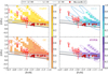 |
Fig. 7 Same as Fig. 6 but in the [O/Fe]–[Fe/H] space. |
| In the text | |
|
Fig. 8 Same as Fig. 6 but in the log(N/O)- log(O/H) + 12 space. Nitrogen and oxygen abundances for the unmixed RGB stars of Mucciarelli et al. (2022) have been derived as described in Sect. 2.1.1. |
| In the text | |
|
Fig. 9 Same as previous figure but for carbon. Carbon and oxygen abundances for the unmixed RGB stars of Mucciarelli et al. (2022) have been derived as described in Sect. 2.1.1. |
| In the text | |
|
Fig. 10 Theoretical log(N/O) versus log(O/H)+12 for a proto-MW galaxy seen at different redshifts. Density maps and contours refer to the predictions of the stochastic GCE model, while the solid lines refer to the predictions of the homogeneous GCE model. Abundances measured in GN-z11 (z = 11, Bunker et al. 2023; Cameron et al. 2023; Senchyna et al. 2024), CEERS-1019 (z = 8.6, Marques-Chaves et al. 2024), and RXCJ2248-ID (z = 6, Topping et al. 2024) are also shown for comparison (symbols and shaded areas). |
| In the text | |
|
Fig. 11 Chemical enrichment of GN-z11. Left and middle panels: predicted log(N/O) versus log(O/H)+12 for GN-z11. Different evolutionary tracks represent different Pop III star-forming clumps, which merge into the main branch of the galaxy. The tracks are color coded according to time elapsed since the beginning of star formation (left) and stellar mass (middle). The light purple trapezoid, the dark purple rectangle, and the gray stripe represent the conservative and fiducial results for the abundances of GN-z11 by Cameron et al. (2023). The blue points are the photoionization modeling results for GN-z11 by Senchyna et al. (2024). Right panel: star formation history of GN-z11 according to Tacchella et al. (2023, red line and shaded area) and as adopted in the model (gray line). |
| In the text | |
|
Fig. 12 Predicted log(C/O) versus log(O/H) + 12 for GS-z12. The evolutionary tracks represent different PopIII star-forming clumps that merge into the main branch of the galaxy. The tracks are color coded to indicate the time elapsed since the beginning of star formation (left panel) and the PopIII stellar mass (right panel). Also shown is the measured log(C/O) abundance for GS-z12 as derived by D’Eugenio et al. (2024). The blue marker represents the estimate obtained through a Bayesian modeling of the spectrum, while the gray stripe marks the lower limit derived using the photoionization models of Gutkin et al. (2016). |
| In the text | |
|
Fig. A.1 Chemical density maps for MW analogs seen at different redshifts. The predictions of the classic, homogeneous GCE model (solid lines; see text) are also shown. |
| In the text | |
Current usage metrics show cumulative count of Article Views (full-text article views including HTML views, PDF and ePub downloads, according to the available data) and Abstracts Views on Vision4Press platform.
Data correspond to usage on the plateform after 2015. The current usage metrics is available 48-96 hours after online publication and is updated daily on week days.
Initial download of the metrics may take a while.