| Issue |
A&A
Volume 691, November 2024
|
|
|---|---|---|
| Article Number | A323 | |
| Number of page(s) | 22 | |
| Section | Cosmology (including clusters of galaxies) | |
| DOI | https://doi.org/10.1051/0004-6361/202450193 | |
| Published online | 22 November 2024 | |
The e-MANTIS emulator: Fast and accurate predictions of the halo mass function in f(R)CDM and wCDM cosmologies
1
Laboratoire Univers et Théories, Université Paris Cité, Observatoire de Paris, Université PSL, CNRS,
92190
Meudon,
France
2
Donostia International Physics Center (DIPC),
Paseo Manuel de Lardizabal, 4,
20018,
Donostia-San Sebastián,
Gipuzkoa,
Spain
3
Sorbonne Université, CNRS, UMR 7095, Institut d’Astrophysique de Paris,
98 bis bd Arago,
75014
Paris,
France
4
Institut universitaire de France (IUF),
France
★ Corresponding author; This email address is being protected from spambots. You need JavaScript enabled to view it.
Received:
31
March
2024
Accepted:
30
September
2024
Abstract
Aims. In this work, we present a novel emulator of the halo mass function (HMF), which we implemented in the framework of the e-MANTIS emulator of f(R) gravity models. We also extended e-MANTIS to cover a larger cosmological parameter space and to include models of dark energy with a constant equation of state wCDM.
Methods. We used a Latin hypercube sampling of the wCDM and f(R)CDM cosmological parameter spaces, over a wide range, and carried out a large suite of more than 10 000 N-body simulations with a different volume, mass resolution, and random phase for the initial conditions. For each simulation in the suite, we generated halo catalogues using the friends-of-friends (FoF) halo finder, as well as the spherical overdensity (SO) algorithm for different overdensity thresholds (200, 500, and 1000 times the critical density). We decomposed the corresponding HMFs on a B-spline basis, while adopting a minimal set of assumptions on their shape. We used this decomposition to train an emulator based on Gaussian processes.
Results. The resulting emulator is able to predict the HMF for redshifts ≤1.5 and for halo masses Mh ≥ 1013 h−1 M⊙. The typical HMF errors for SO haloes with ∆ = 200c at ɀ = 0 in wCDM (respectively f(R)CDM) are of the order of ϵ0 ≃ 1.5% (ϵ0 ≃ 4%) up to a transition mass Mt ≃ 2 ⋅ 1014 h−1 M⊙ (Mt ≃ 6 ⋅ 1013 h−1 M⊙). For larger masses, the errors are dominated by the shot noise and scale as ϵ0 ⋅ (Mh/Mt)α with α ≃ 0.9 (α ≃ 0.4) up to Mh ~ 1015 h−1 M⊙. Independently of this general trend, the emulator is able to provide an estimation of its own error as a function of the cosmological parameters, halo mass, and redshift. We have performed an extensive comparison against analytical parametrizations and shown that e-MANTIS is able to better capture the cosmological dependence of the HMF, while being complementary to other existing emulators.
Conclusions. The e-MANTIS emulator, which is publicly available, can be used to obtain fast and accurate predictions of the HMF in the f(R)CDM and wCDM non-standard cosmological models. As such, it represents a useful theoretical tool to constrain the nature of dark energy using data from galaxy cluster surveys.
Key words: gravitation / methods: numerical / galaxies: clusters: general / cosmology: theory / dark energy / large-scale structure of Universe
© The Authors 2024
 Open Access article, published by EDP Sciences, under the terms of the Creative Commons Attribution License (https://creativecommons.org/licenses/by/4.0), which permits unrestricted use, distribution, and reproduction in any medium, provided the original work is properly cited.
This article is published in open access under the Subscribe to Open model. This email address is being protected from spambots. You need JavaScript enabled to view it. to support open access publication.
1 Introduction
Surveys of the large-scale structures such as the Euclid mission (Amendola et al. 2018), the Dark Energy Spectroscopic Instrument (DESI) experiment (DESI Collaboration 2016), or the Legacy Survey of Space and Time (LSST) at the Vera Rubin Observatory (Ivezić et al. 2019) will map the distribution of galaxies and probe the clustering of matter in the universe over an unprecedented range of scales and redshifts. There is a widespread consensus that these observations can provide insights into the nature of dark energy and test the validity of general relativity (GR) on cosmic scales (see e.g. Joyce et al. 2016, for a review). However, this requires theoretical model predictions capable of accounting for the effects of the non-linear gravitational collapse of matter at late times and at small scales. Unlike linear perturbation theory, accurate predictions of such effects require the use of large volume high-resolution N -body simulations. Nevertheless, a single simulation can only provide predictions for a given cosmological model and more specifically the set of cosmological parameters assumed in the simulation. Given their large computational cost, this poses a challenge to future cosmological parameter inference analyses of large-scale structure data.
Different approaches have been developed to address this issue. Semi-analytical methods, relying on a combination of theoretical modelling and calibration to simulations, have been used to compute the non-linear matter power spectrum (see e.g. Smith et al. 2003; Takahashi et al. 2012; Vlah et al. 2016; Cataneo et al. 2019; Bose et al. 2023) or the halo mass function (HMF; see e.g. Sheth & Tormen 1999; Tinker et al. 2008; Cataneo et al. 2016; Castro et al. 2021). These have the advantage of providing cosmological model predictions at negligible computational costs. Alternatively, approximate numerical schemes have been introduced to perform simplified fast numerical simulations (e.g. Monaco et al. 2002; Tassev et al. 2013). However, these approaches all come with their own limitations and uncertainties that should be propagated in cosmological data analyses. In the last decade, the use of machine-learning algorithms have led to a third way based on the concept of emulators, initially proposed in the seminal work by Habib et al. (2007). Their use of large-scale structure data analyses has become commonplace (e.g. Euclid Collaboration 2019b; Euclid Collaboration 2021; Angulo et al. 2021; Moran et al. 2023; Storey-Fisher et al. 2024).
In fact, cosmological emulators have proven to be very promising tools, as in theory they can be arbitrarily precise and incorporate as many effects as their training dataset provides. While this increase in precision may come at a higher computational cost of generating the training dataset, the resulting emulator is able to provide extremely fast and accurate predictions, which gives them excellent performance when placed within a likelihood designed for a Markov chain Monte Carlo (MCMC) analysis.
In this work, we present an emulator of the HMF, which we implemented within the wider framework of the e-MANTIS1,2,3 emulator of f (R)CDM models (Sáez-Casares et al. 2023); we extended it to a larger cosmological parameter space and included models of dark energy with constant equation of state wCDM. In recent years, the increasing availability of simulations of larger volumes and higher resolutions has led to parametrizations of the HMF providing evermore precise fits to simulations, which are capable of providing better descriptions of the mass, redshift, and cosmological parameter dependence (e.g. Jenkins et al. 2001; Crocce et al. 2010; Courtin et al. 2011; Angulo et al. 2012; Watson et al. 2013; Despali et al. 2016; Bocquet et al. 2016; Diemer 2020; Ondaro-Mallea et al. 2022; Castro et al. 2021). These parametrizations have since been used as a core part of cosmological studies, such as cluster number count analyses (Allen et al. 2011; Kravtsov & Borgani 2012; Rozo et al. 2010; Mantz et al. 2015; de Haan et al. 2016; Planck Collaboration XXIV 2016; Schellenberger & Reiprich 2017; Pacaud et al. 2018; Bocquet et al. 2019; Abbott et al. 2020; Costanzi et al. 2021; Lesci et al. 2022), which are rapidly gaining traction due to the increasing size of the cluster samples to which the community has, and will have, access (e.g. Hofmann et al. 2017; Euclid Collaboration 2019a; Raghunathan et al. 2022). Nonetheless, in the current era of precision cosmology, several of the previous fitting functions have become insufficiently accurate given survey and mission requirements (see e.g. Bocquet et al. 2016; Castro et al. 2021) or they are simply unable to explore the wider parameter space of cosmological models considered. This motivates the development of dedicated emulators capable of accurately predicting the HMF for different cosmological scenarios and cosmological parameter values. A number of emulators of the HMF in wCDM models have already been developed in the literature (see e.g. Nishimichi et al. 2019; McClintock et al. 2019; Bocquet et al. 2020). However, some of them (such as McClintock et al. 2019), are limited to a narrow emulation range around current observational constraints. Additionally, existing wCDM HMF emulators usually only support a single dark matter halo definition, which is not necessarily the same as the ones used in usual observational analyses. In the case of f (R)CDM cosmology, the only existing emulator for the HMF is the one presented in Ruan et al. (2023). This emulator does not cover the mass range of galaxy clusters, since it is aimed at modelling galaxy clustering. Here, we present a novel emulator that supports multiple dark matter halo definitions commonly used in both theoretical and observational studies. It covers a wider parameter space than existing wCDM emulators, and it is the first emulator for the f (R)CDM cosmologies in the galaxy cluster mass range.
This paper is structured as follows. Section 2 presents the extended e-MANTIS N-body simulation suite. Section 3 explains the methodology employed to emulate the HMF. In Sect. 4 we validate the predictions of the emulator and compare them to external simulations and other publicly available predictions.
2 The extended e-MANTIS simulation suite
2.1 Alternative dark energy models
In the standard cosmological scenario, the cosmological constant Λ is equivalent to a homogeneous static fluid characterized by an equation of state w = –1 corresponding to a constant energy density. By contrast, a dynamical form of dark energy can be described as a fluid with a constant equation of state w ≠ –1 provided that w < –1/3, such as to ensure it sources the cosmic acceleration. In such a case, the dark energy density evolves as a power-law function of redshift, that is, ρDE ∝ (1 + z)3(1+w). Models with –1 < w < –1/3 can approximate the dynamics of quintessence scalar field scenarios (Caldwell et al. 1998), while models with w < –1 corresponds to the so-called phantom dark energy scenario (Caldwell et al. 2003), that can also mimic unaccounted scalar interactions between dark energy and dark matter (Das et al. 2006). As such, the wCDM model is a simpler realization of dynamical dark energy scenarios.
Alternatively, dark energy may result from a modification of Einstein’s theory of GR on cosmic scales (see e.g. Nojiri & Odintsov 2011; Clifton et al. 2012; Nojiri et al. 2017). One popular example of modified gravity (MG) is the f (R) gravity model (see e.g. Sotiriou & Faraoni 2010). This takes the form of a modification of the Einstein-Hilbert action by the addition of a function f of the Ricci scalar R:
![Mathematical equation: ${S_g} = {1 \over {2{\kappa ^2}}}\int {{{\rm{d}}^4}} x\sqrt { - g} [R + f(R)],$](/articles/aa/full_html/2024/11/aa50193-24/aa50193-24-eq1.png) (1)
(1)
with κ2 = 8πG/c4 where G is Newton’s constant, c the speed of light in vacuum, and g the determinant of the space-time metric 𝑔μv Here, we focus on a specific f(R) gravity model proposed by Hu & Sawicki (2007), which assumes
 (2)
(2)
where c1, c2 and n are dimensionless parameters, and m is a curvature scale. The latter is set to
 (3)
(3)
where Ωm is the cosmic matter density today and H0 the Hubble rate. The coefficient c1 and c2 can be set to
 (4)
(4)
such that in the high curvature limit (R >> m2) the model matches the accelerating phase of the ΛCDM model. Hence, in such a limit, the function f reads as
 (5)
(5)
where  is the derivative of the scalar function with respect to the Ricci scalar evaluated at z = 0. At the level of the background expansion,
  is a parameter that sets the deviation with respect to w = –1 of the cosmological constant case (Hu & Sawicki 2007). Here, we consider f (R) gravity models characterized by deviations from GR no greater than
  . From a phenomenological point of view, these models have a background expansion indistinguishable from that of the ΛCDM model, with negligible differences concerning the evolution of the matter density perturbations at high redshift. On the other hand, differences arise in the late-time non-linear regime of cosmic structure formation, thus requiring the use of numerical simulations.
Here, we consider f (R)CDM models with n = 1. We remark that an emulator of the matter power spectrum for models with n , 1 has been developed using an approximate N -body solver (Ramachandra et al. 2021). This is because N-body simulations of f (R) models with n , 1 are significantly more time-consuming than the case n = 1 (see Bose et al. 2017). However, this approach is not sufficiently accurate at the level we wish to capture on non-linear scales. Henceforth, as a starting point to build an accurate and efficient emulator of f (R) gravity models, we focus on the case n = 1 and we leave the extension to n , 1 to future work. We note that a simple particle-mesh solver has been developed by Ruan et al. (2022), to simulate the nonlinear clustering of matter in the cases n = 0 and n = 2, which also benefit from the same speed-up as n = 1.
Ranges of the cosmological parameters supported by the emulator, and values of the cosmological parameters for some reference models.
2.2 Cosmological parameter space
In the case of the wCDM scenario, dark energy is specified by the value of a constant equation of state parameter, w. In the case of the f (R)CDM scenario, the amplitude of the gravity modifications relative to GR is specified by the value of  . The rest of the parameter space for both scenarios is specified by the values of the standard cosmological parameters: the total matter density Ωm, the scalar spectral index ns, the reduced Hubble rate h4, the baryon density parameter Ωb, and the amplitude of linear matter density fluctuations on the 8 h–1 Mpc scale
  in GR. By
  , we refer to the σ8 obtained assuming a linear GR evolution. In the case of wCDM, this corresponds identically to the usual σ8. In the case of f (R)CDM, we follow the usual convention where
  corresponds to the value of σ8 in ΛCDM with identical cosmological parameters other than
  . We assume a flat geometry, we ignore massive neutrinos, and set the radiation density parameter to the value given by the cosmic microwave background (CMB) temperature, Ωr ~ 10–4.
It is worth stressing that the predictions from emulators are limited to the range of parameters initially selected to generate the training set. Extending the emulator to a wider range or to support additional parameters is not straightforward, as it usually requires restarting the whole procedure. Because of this, it is important for an emulator to have a sufficiently large parameter space (larger than current cosmological constraints) to be effectively used for observational data analyses. A large range is also needed in order to capture the subtle deviations from universality of the dark matter HMF (Tinker et al. 2008; Courtin et al. 2011; Ondaro-Mallea et al. 2022). On the other hand, considering a too large parameter space may lead to a lower density of training points and consequently degrade the final accuracy of the emulator. Guided by the choice made in previous emulators of wCDM and f (R)CDM models, we consider the following range of values for w and  respectively: w ∈ [–1.5, –0.5] and
 ![Mathematical equation: ${\log _{10}}\left| {{f_{{R_0}}}} \right| \in [ - 7, - 4]$](/articles/aa/full_html/2024/11/aa50193-24/aa50193-24-eq19.png) ; while we set the range of the other cosmological parameters to the following values: Ωm ∈ [0.155, 0.465],
; while we set the range of the other cosmological parameters to the following values: Ωm ∈ [0.155, 0.465], ![Mathematical equation: $\sigma _8^{{\rm{GR}}} \in [0.608,1.014]$](/articles/aa/full_html/2024/11/aa50193-24/aa50193-24-eq20.png) , h ∈ [0.55, 0.85], ns ∈ [0.72, 1.20], and Ωb ∈ [0.037, 0.064]. These values are summarized in Table 1.
, h ∈ [0.55, 0.85], ns ∈ [0.72, 1.20], and Ωb ∈ [0.037, 0.064]. These values are summarized in Table 1.
The ranges we consider are wider than those assumed in existing emulators of the HMF for wCDM models (see e.g. McClintock et al. 2019; Nishimichi et al. 2019). This is also the case of the Mira-Titan emulator (Bocquet et al. 2020), for which we consider a larger range of values of w. On the other hand, the Mira-Titan emulator supports the case of massive neutrinos and a time-varying equation of state, which we do not include here.
As far as the emulators of f (R)CDM models are concerned, the N -body simulation suite used here is the first to fully explore the 6-dimensional cosmological parameter space of such models. As an example, the FORGE N -body simulation suite (Arnold et al. 2022) does not include variations of the scalar spectral index ns and the baryon density parameter Ωb, and has a more restricted range in terms of the  parameter. The approximate simulations presented in Ramachandra et al. (2021) do not take into account the reduced Hubble constant h, although they consider variations of the n parameter. In this work, we extend the base of parameters sampled in the first version of the e-MANTIS emulator presented in Sáez-Casares et al. (2023), to include the dependence on ns, h, and Ωb, while sampling a wider interval of Ωm values.
2.3 Sampling the parameter space
A common approach to efficiently sample the multidimensional cosmological parameter space with a reduced number of N -body simulation consists in using a Latin hypercube sampling (LHS) method (McKay et al. 1979). Such a strategy has been shown to provide accurate emulators when combined with Gaussian processes (GP) (Habib et al. 2007).
In order to sample a parameter space with N points, the LHS method first divides the D-dimensional parameter space with a ND regular grid. Then, N random cells are selected, with the constraint that any two cells cannot have any common coordinates. The space filling properties of the LHS can be further improved by applying different optimizations, such as maximizing the minimum distance between points (maximin-distance condition). One limitation of the simple LHS approach, is that once a sample of N points has been selected, there is no direct way of adding new points. In practice, it is usually difficult to know in advance the exact number of simulations necessary to achieve a satisfactory level of emulation accuracy. One possibility is to use approximate analytical models as surrogate training data to determine the number of cosmological models which need to be sampled. However, this would only apply to a given particular observable.
In the work of Sheikholeslami & Razavi (2017), the authors have introduced a method to generate a progressive Latin hypercube sampling (PLHS). A PLHS generates multiple sub-sets (slices) of points, such that each slice is a LHS and the progressive union of all slices remains a LHS at all stages. It is possible to generate as many new slices as desired. However, building a PLHS requires doubling the number of points with each new slice. This procedure becomes impractical in the context of expensive numerical simulations and does not allow a fine control of the final number of training models. These issues can be somewhat alleviated through the use of a quasi-PLHS, which we use to construct our training data set. As such, we briefly introduce the main aspects of the quasi-PLHS method below, but refer the interested reader to Sheikholeslami & Razavi (2017) for more details.
The quasi-PLHS method is based on the sliced Latin hypercube sampling (SLHS) method. A SLHS is an ensemble of a finite number of LHS slices, the union of which also forms a LHS. However, the progressive union of slices does not constitute a LHS at each step, as would be the case with a perfect PLHS. An example of a method to generate an SLHS is presented in Ba et al. (2015). The main idea behind the quasi-PLHS is to find an optimum ordering of the slices, so that their progressive union is as close as possible to a LHS. Using this method, it is possible to progressively increase the number of points in the sample with an arbitrary constant step up to a maximum number of points fixed in advance. By fixing the maximum number of points to a sufficiently large value, it is possible to add as many models as needed to the training samples progressively. The price to pay for a more flexible sampling method, is that for a given number of slices, the distribution of points is less optimal than a one-shot LHS of the same size. The only cases where we obtain a real LHS, is either by using a single slice or all of them.
We generated a maximin-distance SLHS following the method introduced by Ba et al. (2015). The optimized distance is a combination of the distance between points in each slice and in the union of all slices. We used the R package SLHD5 to generate 16 slices with 16 points each, resulting in 256 models. The total number of 256 models is a conservative upper limit, since most cosmological N-body based emulators do not use that many training simulations. We then used the quasi-PLHS method of Sheikholeslami & Razavi (2017) to find an optimum ordering of the slices. At the current stage, we have run N -body simulations for the first 5 slices (i.e. 80 models). The other 11 slices remain available for future extension of the simulation suite. Figure A.1 shows the final distribution of cosmological models in both f (R)CDM and wCDM. In both models, we use exactly the same values of Ωm,  , ns, h, and Ωb. For w and
  , we use the same distribution of points, which is simply scaled to their respective range of values.
2.4 Simulation pipeline
The simulation suite presented in this work has been run using the automated simulation pipeline described in Sáez-Casares et al. (2023), which is an extension to f (R) gravity models of the original wCDM pipeline developed for the Parallel-UniverseRuns (PUR) project (Blot et al. 2015, 2021). Compared to the original version of the simulation pipeline, several improvements have been implemented. We describe here the updated pipeline used in this work.
The linear matter power spectra necessary to the generation of initial conditions were computed using CAMB (Lewis et al. 2000). The initial conditions, particle displacements, and velocities, were generated using a modified version of the code MPgrafic (Prunet et al. 2008), which computes the displacement field with second-order Lagrangian perturbation theory. The starting redshift was taken as late as possible while avoiding particle crossing (i.e. zi ∼ 50) in order to minimize discreteness errors (Michaux et al. 2021). The dark matter particles have been evolved with the code ECOSMOG (Li et al. 2012; Bose et al. 2017), a modified gravity version of the Adaptive Mesh Refinement N- body code RAMSES (Teyssier 2002; Guillet & Teyssier 2011). We have modified ECOSMOG in order to solve the Poisson equation for the sum of the two Bardeen potentials (ϕ and ψ), which is relevant for future weak-lensing studies. Finally, the matter power spectra have been computed with the code POWERGRID (Prunet et al. 2008).
Haloes were detected using two distinct halo finder codes: pFoF, a parallelized version of the friends-of-friends (FoF) percolation algorithm described in Roy et al. (2014); pSOD, a parallelized version of the spherical overdensity (SO) algorithm (Lacey & Cole 1994) based on the pFoF parallel scheme. In the case of the SO halo finder, the cloud-in-cell (CIC) density of all particles is computed on a grid twice thinner than the coarse grid of the dynamical solver. Only ’dense’ particles with density larger than 120 times the matter density are selected as possible candidates for halo centres. We note that decreasing this threshold does not change the final result. The selected particles are then considered in decreasing density order. For each particle considered, we scan all particles which belong to the same coarse cell and those in the 124 neighbouring cells to find the particle with the lowest value of the gravitational potential, as computed by ECOSMOG. In previous versions, the centre was identified as the position of the densest particle or the location of the minimum of the self-binding energy. Once the centre is found, a sphere of increasing radius is grown outwards until the average density within the sphere, including all particles, drops below a given density threshold. Finally, all the particles within the sphere are removed from the list of possible centres and the process is repeated. We stored the particles of each detected halo, thus allowing us to compute various halo properties in a post-processing step.
2.5 The N -body simulation suite
The extended e-MANTIS simulation suite consists of simulations of different cosmological models that pave the parameter space of the wCDM and f (R)CDM models. For each of the sampled models, the suite includes simulations of different volume, mass resolution, and number of independent realizations. In this subsection, we describe the main characteristics of these simulations, which are summarized in Table 2.
The core set of simulations, which are used to train the emulators, sample 80 cosmological models using the strategy described in Sect. 2.3, both in wCDM and f (R)CDM. For each cosmological model, we used two different simulation volumes, a smaller box of side length Lbox = 328.125 h–1 Mpc (hereafter L328) and a larger box of side length Lbox = 656.25 h–1 Mpc (hereafter L656). In both cases we used 5123 N-body particles, resulting in a particle mass resolution of mpart ∼ 1010 h−1 M⊙ (hereafter M10) and mpart ~ 1011 h–1 M⊙ (hereafter M11) respectively. We note that the exact particle mass depends on the value of Ωm used in the simulation (see Table 2). The resolution of the L328_M10 simulations is sufficient to resolve group sized haloes (see Sect. 3.2 and Appendix B), while the volume of the L656_M11 set provides sufficient statistics to study the abundance of cluster sized haloes. The systematic error on the high mass end of HMF due to the finite volume of the L656 box is smaller than ~2% up to halo masses of Mh ≲ 1015 h–1 M⊙(Euclid Collaboration 2023). This is negligible with respect to the Poisson noise (see Fig. 4). For each cosmological model and each box-size, we ran 64 independent realizations in the case of wCDM and 8 in the case of f (R)CDM, as the computation is much more intensive in the latter case. We thus reached an effective volume of 2625 h–1 Mpc per cosmological model in wCDM, and (1312.5 h–1 Mpc)3 in f(R)CDM. The initial conditions are common to all cosmological models. The random phases of the initial conditions were designed such that each group of 8 realizations of the L328_M10 simulations correspond to the same random phase as one of the L656_M11 simulations. This means that the first L656_M11 realizations bring no additional information with respect to the whole set of L328_M10 simulations. However, we can use this matching to correct for finite mass resolution errors in the L656_M11 simulations, and for each individual cosmological model.
In addition to this core set, we ran higher resolution simulations with 10243 N -body particles for both the L328 and L656 box-sizes, which correspond to a particle mass resolution of mpart ~ 109 h–1 M⊙ (hereafter M9) and mpart ~ 1010h–1M⊙(M10) respectively. We used these simulations to correct for finite mass resolution effects. We ran these simulations only for a single realization and only for the first slice of our wCDM quasi-PLHS, which corresponds to a perfect LHS with 16 models. Therefore, it is possible to partially explore the cosmological dependence of such finite mass resolution effects in wCDM.
We ran additional simulations for some reference cosmological models. In particular, we considered a Planck Collaboration VI (2020) compatible ΛCDM cosmology (hereafter P18), with Ωm = 0.3071,  , h = 0.6803, ns = 0.96641, and Ωb = 0.048446. We also considered a reference wCDM cosmology with w = –1.2 (hereafter w12) and a reference f (R)CDM model with
  (hereafter F5). In both cases, the other cosmological parameters take the values of the P18 model. The values of these cosmological parameters are summarized in Table 1. We ran 384 independent realizations of the L328_M10 box for P18 and 64 realizations for w12 and F5. These simulations were not used during the emulator training and serve only as a validation set.
Finally, we ran another set of simulations in order to study the numerical convergence in terms of mass resolution for some selected reference models. This last set uses a box-size of Lbox = 164.0625 h–1 Mpc (hereafter L164), with2563, 5123, and 10243 N -body particles, corresponding to a particle mass resolution of mpart ~ 1010h–1M⊙(M10),mpart ~ 109h–1M⊙(M9), and mpart ~ 108 h–1 M⊙ (hereafter M8) respectively. We ran a single realization for the P18 cosmology for each of these resolutions, and for the F5 and F6 cosmologies for the M10 and M9 resolutions.
We stored all the particles of the simulation snapshots, as well as the particles of FoF and SO haloes at 11 redshifts: z = {zi ~ 49, 2.6, 2, 1.5, 1.25, 1, 0.7, 0.5, 0.25, 0.1, 0}. We saved the particle positions and velocities, as well as the values of the two Bardeen potentials (ϕ and ψ), and the value of the fR field interpolated at the position of each particle. Additionally, we stored the matter power spectra and halo profiles, as well as some other basic halo properties, for both FoF and SO haloes at 23 redshift outputs: z = {zi ~ 49, 3, 2.6, 2.3, 2, 1.74, 1.5, 1.4, 1.25, 1.1, 1, 0.9, 0.7, 0.6, 0.5, 0.42, 0.3, 0.25, 0.15, 0.1, 0.05, 0}.
Summary of the main characteristics of the different simulation sets used in this work.
3 Emulating the HMF
The halo mass function quantifies the number of haloes of a given mass in an infinitesimal comoving volume. The seminal work by Press & Schechter (1974) provided the first analytical derivation of the HMF within the hierarchical bottom-up CDM scenario of cosmic structure formation. Subsequently, Bond et al. (1991) formulated a stochastic model to predict the HMF in a given cosmological scenario. However, the discrepancy between the analytical predictions and the results of simulations has led to the development of a phenomenological approach driven by fitting parameterized functions to the results of N-body simulations. Building upon the work of Sheth & Tormen (1999), over the last two decades numerous works in the literature have presented calibrated parametrization of the HMF improving on the resolution and volume of N -body simulations with the intent of better capturing its mass, redshift, and cosmology dependence.
The advent of a new generation of galaxy cluster surveys has triggered novel effort in the development of fast and accurate predictions of the HMF. The realization of emulators capable of providing predictions accurate at the level required to perform unbiased cosmological analyses for a wide range of cosmological parameter values and different cosmological scenarios is therefore timely. Here, we will present the simulation training data and the HMF emulation algorithm implemented in the e-MANTIS emulator.
3.1 The HMF training data
We detected FoF dark matter haloes with a linking length of b = 0.2 (in units of the mean interparticle distance), and SO haloes with an overdensity threshold of ∆ = 200 times the critical density of the universe (hereafter 200c). From the density profiles of the SO haloes detected with ∆ = 200c, we computed for each halo their mass at the overdensity thresholds ∆ = 500c and ∆ = 1000c. We used these additional conditional mass measurements as new halo definitions. We estimated the halo mass function, dn/dln Mh, for all these halo definitions, with constant logarithmic mass bins of width ∆ log10 Mh ≃ 0.05. Halo masses are given in units of h–1 M⊙, thus implying that the HMF has units of h3 Mpc–3, where Mpc denotes comoving megaparsec.
The HMF emulator training data was built by combining the HMF measurements from the simulation boxes L328_M10 and L656_M11 of the emulator set (see Sect. 2.5). More specifically, we considered a minimum mass in the small volume simulations of Mh,min = 5 ⋅ 1012 h–1M⊙ in the case of FoF haloes, while in the case of the SO haloes we set Mh,min = 1013 h–1M⊙. These values correspond to haloes with ∼150 and ∼300 particles, respectively, for the models with the worst mass resolution (corresponding to cosmologies with Ωm = 0.465). As shown in Sect. 3.2, this is the minimum number of particles for which it is possible to apply a cosmology independent mass resolution correction. We used the L328_M10 HMF up to a mass corresponding to haloes with Npart,M11 = 2000 low resolution particles (i.e. Npart,M10 = 16 000 high resolution particles), and switch to the L656_M11 HMF for haloes with a larger number of particles. We found that this threshold ensures a smooth transition from one simulation box to the other. Any residual systematic difference was compensated by the resolution correction introduced in Sect. 3.2. We forced a minimum number of 5 haloes per bin by merging high mass end bins. For each cosmological model θi, we halted the computation of the HMF at a maximum mass Mh,max,i, corresponding to the mass bin in which the criterion can no longer be satisfied. We estimated the errors on the HMFs by using 1000 bootstrap random catalogues.
3.2 HMF mass resolution correction
In order to both improve the accuracy of the L328_M10 training data at the low mass end, and to smooth out the transition between the L656_M11 and the L328_M10 simulation boxes, we computed a correction for the finite mass resolution errors in the HMF measurements. We defined the correction as the ratio of the HMF measured from a simulation with a higher resolution MX (i.e. a lower particle mass) to the HMF measured from a lower resolution MY (i.e. a higher particle mass), with X < Y. In practice, we do not dispose of high resolution simulations for all the cosmological models and realizations of our simulation suite. As such, the first approximation we employed, is to assume that the correction will be independent of the specific realization. Additionally, we find that when the correction is expressed in terms of the low resolution number of particles per halo Npart,MY, instead of the halo mass Mh, the correction is independent of the cosmological model. This approximation holds up to a certain minimum number of particles per halo. A direct consequence is that we can average the HMF ratio over multiple cosmological models in order to reduce the measurement noise. It is also possible to apply the correction computed on a subset of cosmological models to all the training data of the emulator simulation set. Furthermore, in order to obtain a smooth correction, we fitted an analytical function to the measured HMF ratio averaged over all available cosmological models and realizations. In the case of SO haloes, we used the following fitting function for the ratio of the HMF with the higher resolution MX and the HMF with the lower resolution MY
 (6)
(6)
where N0 and σ0 are free dimensionless parameters. In the case of FoF haloes, we modified the fitting function as
 (7)
(7)
where c is an additional free dimensionless parameter.
In order to improve the accuracy of the HMF training data at the low mass end, we computed this type of correction for the L328_M10 simulation boxes of the emulator training set. To do so, we measured the corresponding HMF ratio using the L328_M9_wcdm simulation set described in Sect. 2.5. Figure 1 shows the HMF ratios for the 16 cosmological models of the first wCDM quasi-PLHS, along with their mean and standard deviation, for different halo definition and redshifts. We also computed the expected error on each HMF ratio using 43 spatial jackknife sub-volumes. The different cosmological models have different errors. For simplicity, we averaged all the errors in quadrature, which are shown in Fig. 1 attached to the mean HMF ratio. This mean error is indicative of the typical expected statistical noise in each HMF ratio. Its agreement with the standard deviation between the different models is indicative of the cosmological independece of the mass resolution correction.
We found that the mass resolution correction is cosmology independent for FoF haloes with b = 0.2 and Npart,M10 ≳ 150 and SO haloes with ∆ = 200c, ∆ = 500c and Npart,M10 ≳ 300. For a smaller number of particles, we found large deviations from one cosmology to another (not shown in Fig. 1). Since we want to average the HMF ratio over all cosmologies in order to reduce the noise in the signal, this observation motivates the minimum mass supported by the emulator (see Sect. 3.1). We stress the fact that the 16 cosmological models considered form a perfect LHS, and therefore explore the whole 6-dimensional wCDM parameter space, albeit with a reduced number of points. In the case of SO haloes with ∆ = 1000c, the measurements are noisier, which makes it more difficult to conclude on the cosmological dependence. However, considering a correction beyond the mean cosmological HMF ratio would require larger volume simulations or more realizations of the high resolution L328_M9 box. We decided to keep the same minimum number of particles per halo as for the other overdensity thresholds, that is, Npart,M10 ≳ 300.
In the case of SO haloes, the HMF ratio has the shape of a decreasing exponential, converging towards unity at large number of particles per halo. This feature is mainly due to the dynamical solver of the N-body code, which, because of the finite resolution, tends to underestimate the clustering at small scales (see e.g. Rasera et al. 2014). In the case of FoF haloes, the HMF ratio does not converge to unity even at large number of particles per halo. There is a residual shift of a few percent. Indeed, FoF haloes are affected by an additional resolution effect. As pointed out by More et al. (2011), the FoF algorithm tends to overestimate the mass of a halo if the resolution of the simulation is not sufficient (i.e. if the halo is not sampled by enough particles). Our interpretation is that, for small haloes, the error from the dynamical solver dominates. When this component converges to unity, the opposite error due to the FoF algorithm has not yet converged. This makes the HMF ratio crossing the unity line. Eventually, the HMF ratio should converge to one. However, the convergence is slow and our data is noisy at the high mass end. We decided to approximate this regime by a constant, corresponding to the extra parameter in the fitting formulan given in Eq. (7) with respect to the SO case. In practice, we never used the correction for haloes larger than the last data point for which were able to measure the HMF ratio, since the mass range of the emulator does not go beyond that.
We fitted the analytical forms of Eqs. (6) and (7) to the mean HMF ratio, independently for each halo definition and redshift. The resulting correction, which is also shown in Fig. 1, was applied to all the HMF training data of both wCDM and f (R)CDM emulators. In Appendix B, we show that even if this correction has been computed from wCDM simulations, it remains valid in the case of f (R) gravity. We also test the numerical convergence of the correction.
Although the transition between the simulation boxes L328_M10 and L656_M11 takes place at a high number of low resolution number of particles per halo (see Sect. 3.1), we found that in some cases a small residual systematic difference remains. This produces a discontinuity in our HMF training data, which degrades the accuracy of the final emulator. In principle, we could use the L656_M10_wcdm simulation set, to compute the same kind of correction as described in the last paragraph. However, in this case the HMF ratio is significantly noisier, since we are interested in more massive haloes. The larger volume of the L656 simulation box with respect to the L328 box does not compensate the drop of the HMF. Therefore, even by averaging the HMF ratio over the 16 cosmological models of the L656_M10_wcdm set, the measurements are too noisy to perform a proper fit at all redshifts. Instead, we used of the initial condition matching between the L328_M10 and the L656_M11 simulation sets described in Sect. 2.5. In this case, we can compute the mean correction using 80 cosmological models instead of 16, and therefore obtain a smoother measurement. We computed the ratio of the HMF measured using all the realizations from L328_M10 and the HMF from the L656_M11 realizations corresponding to the same initial random phase, both in wCDM and f(R)CDM. We performed the same kind of fit to the mean HMF ratio and apply the obtained correction to all the measurements from the L656_M11 simulation box. We found that, in the case of SO haloes, at the transition between both simulations volumes, that is, for a number of low resolution particles per halo of Npart,M11 = 2000, the L656_M11 HMF has converged to the L328_M10 HMF within the statistical noise of the training data. Therefore, the transition between both simulation volumes is smooth without the need to correct the resolution of the larger volume simulations. This is due to the fact that we have chosen to only use the L656_M11 data for sufficiently massive haloes. We still applied the correction, both for consistency and to remove any residual errors. However, in the case of FoF haloes, we observed the same kind of systematic shift at large number of particles per halo as discussed in the previous paragraph. Therefore, it is essential to correct this effect to properly transition from one simulation volume to the other. We found that if this correction is not applied, the goodness-of-fit of the HMF B-spline decomposition presented in Sect. 3.3 is degraded significantly around the transition, that is, Nparti,M11 ≃ 2000. The HMF ratios and the corresponding mean and fitted function, for the FoF case both in wCDM and f(R)CDM, are shown in Fig. 2.
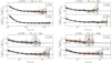 |
Fig. 1 Ratio of the HMF with the better mass resolution M9 to the one with the standard mass resolution M10 as a function of the number of standard resolution particles per halo Npart,M10 at z = 0 and z = 1. This quantity has been computed using the higher resolution simulation set L328_M9. Each sub-plot shows the case of a different halo definition: FoF with b = 0.2 (top-left) and SO with ∆ = 200c (top-right), ∆ = 500c (bottom-left), and ∆ = 1000c (bottom-right). Each coloured line corresponds to one of the 16 cosmological models of the first slice of the wCDM quasi-PLHS. The black solid line gives the mean over all cosmological models, with the standard deviation among them as error bars. The grey band attached to the mean is an estimation of the typical expected error for the individual HMF ratio. The dashed line corresponds to the fit to the mean using the fitting function given in Eq. (6) for SO haloes, and in Eq. (7) for the FoF case. |
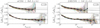 |
Fig. 2 Ratio of the FoF (b = 0.2) HMF with the better mass resolution M10 to the one with the standard mass resolution Mil as a function of the number of standard resolution particles per halo Npart,M11, in wCDM (left) and f(R)CDM (right), at z = 0 and z = 1. This quantity has been computed using the matching in terms of initial conditions between the L656_M11 and the L328_M10 simulation sets. Each coloured line corresponds to one of the 80 cosmological models of the emulator training set. The black solid line gives the mean over all cosmological models, with the standard deviation among them as error bars. The grey band attached to the mean is an estimation of the typical expected error for the individual HMF ratio. The dashed line corresponds to the fit to the mean using the fitting function given in Eq. (7). |
3.3 B-spline decomposition of the HMF
One common approach to emulate the HMF is to first fit the measured HMFs of each cosmological model using some parametric fitting formula. In a second step, the coefficients from the fitted HMFs are emulated to account for their cosmological dependence. As an example, a number of ωCDM emulators of the HMF have assumed the parametrization from Tinker et al. (2008) as fitting function (McClintock et al. 2019; Nishimichi et al. 2019). However, previous studies have shown that this type of approach is not able to accurately capture the shape of the HMF in modified gravity theories at percent level accuracy (see e.g. Schmidt et al. 2009; Lombriser et al. 2013; Gupta et al. 2022). Because of this, we chose a different approach and adopt a fitting strategy that limits the assumptions made about the shape of the HMF. We fitted the numerically estimated HMF by piece-wise polynomials or splines, following a similar procedure to the one used in Bocquet et al. (2020). More specifically, we decomposed the HMF using B-splines, which constitute a basis for spline functions, while the work of Bocquet et al. (2020) used constrained piecewise polynomials.
Formally, a B-spline decomposition is defined by the degree p of the polynomial pieces, the positions tk of the knots (i.e. where the polynomial pieces meet) and the coefficients cj multiplying each B-spline basis function. Consider two boundary knots delimiting the range of the B-spline decomposition and an ensemble of n internal knots, which corresponds to n + 1 polynomial pieces. Constructing the B-spline basis requires p additional knots below the lower boundary knot and another p knots above the upper one (see e.g. Perperoglou et al. 2019). Their values are arbitratry, and they are usually set equal to the lower and upper boundaries, respectively. Once the knots have been fixed, the B-splines of degree p = 0 are defined as
![Mathematical equation: ${B_{j,0}}[x] \equiv \left\{ {\matrix{ 1 \hfill & {{\rm{ if }}{t_j} \le x < {t_{j + 1}},} \hfill \cr 0 \hfill & {{\rm{ otherwise}}{\rm{. }}} \hfill \cr } } \right.$](/articles/aa/full_html/2024/11/aa50193-24/aa50193-24-eq28.png) (8)
(8)
Then, B-splines of degree p > 0 can be constructed by recursion (de Boor 1972)
![Mathematical equation: ${B_{j,p}}[x] \equiv {{x - {t_j}} \over {{t_{j + p}} - {t_j}}}{B_{j,p - 1;{\rm{t}}}}[x] + {{{t_{j + p + 1}} - x} \over {{t_{j + p + 1}} - {t_{j + 1}}}}{B_{j + 1,p - 1;{\rm{t}}}}[x],$](/articles/aa/full_html/2024/11/aa50193-24/aa50193-24-eq29.png) (9)
(9)
for j = 1, ⋯ , n + p + 1. The complete B-spline basis is made up of n + p + 1 functions. Hence, the B-spline decomposition of the estimated HMF reads as
![Mathematical equation: ${\log _{10}}\left[ {{{{\rm{d}}n} \over {{\rm{d}}\ln {M_h}}}} \right] = \mathop \sum \limits_{j = 1}^{n + p + 1} {c_j}{B_{j,p}}\left[ {{{\log }_{10}}{M_h}} \right].$](/articles/aa/full_html/2024/11/aa50193-24/aa50193-24-eq30.png) (10)
(10)
We chose splines of degree p = 2 and knots of logarithmic mass points equally spaced by ∆log10 Mh ≃ 0.25. The only assumption about the shape of the HMF is that it can be described by a polynomial of degree 2 in log-log axes over intervals of ~0.25 dex. The same description of the shape of the wCDM HMF is used in Bocquet et al. (2020). We found that this approach is also able to capture the shape of the HMF in f(R) gravity.
One important aspect of the B-spline decomposition to be considered, is that when fitting the HMF, the maximum mass needs to be the same for all cosmological models, since we want to decompose all the individual HMFs into the same B-spline basis. However, we found that there is up to an order of magnitude difference between the maximum mass of different cosmological models. We set the maximum mass of the B-spline decomposition to
 (11)
(11)
where the average is performed over all cosmological models θi. We found that a value of α = 0.5 gives a good compromise between maximizing the range of the emulator without degrading the quality of the B-spline fit at the high-mass end. This defines the maximum mass range of the emulator at each redshift and for each halo definition, as shown in Fig. 3. Furthermore, it is necessary that for each cosmological model, there is a minimum number of data points per polynomial piece to perform the B-spline decomposition. For this purpose, we merged the high mass internal knots till all the cosmological models have at least three data points in the last spline segment. In Fig. 4, we showed a visual example of the location of the B-spline knots.
We used the Python package SciPy (Virtanen et al. 2020) to perform the spline fitting to the HMFs and included the diagonal errors of the simulation measurements into the fit. We estimated the variance of the spline coefficients by drawing 1000 random HMFs from the estimated simulation noise, and repeating the fitting procedure each time. We repeated this operation for each halo definition and each redshift output of the wCDM and f(R)CDM simulation sets. In Fig. 4, we compare the B-spline fit to the HMF data measured from the simulations for the case of SO haloes with ∆ = 200c at z = 0 for the wCDM and f(R)CDM models respectively. In order to assess the goodness-of-fit, we compute the residuals normalized by the noise in the data in each mass bin. The distribution of the normalized residuals for all training cosmological models as a function of mass is also presented in Fig. 4. As we can see, the 97.7, 84.1, 50, 15.9, 2.3 percentiles closely match the 1 and 2σ levels over the bulk of mass range considered, which is consistent with the expectation of a normal distribution with unit variance. We find no significant degradation of the quality of the B-spline fit due to the merging of the large mass spline intervals. Additionally, we detect no discontinuity at the transition between both simulation boxes, which takes place in the mass range ~(1 – 5) ⋅ 1014 h−1M⊙ depending on the particular cosmological model (see Sect. 3.1). Only at the low-mass end in the wCDM case the residuals are larger than the expected noise of the simulations (~0.1%), nonetheless they remain smaller than 1%. This is because the wCDM simulations have 8 times the number of realizations of the f(R)CDM models, hence the statistical noise of the estimated HMFs is systematically smaller. Therefore, we can conclude that the uncertainties on the B-spline fits are dominated by the noise of the estimated HMF from simulations except some cases at small masses, where uncertainties saturate at ~0.5% level. This shows that the B-spline decomposition accurately describe the HMFs of wCDM and f(R)CDM cosmologies across the mass range of interest with percent level accuracy. We found similar results at higher redshifts, as well as for the other halo definitions considered in this work.
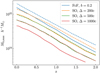 |
Fig. 3 Maximum halo mass range of the f(R) emulator (solid lines) and wCDM emulator (dashed lines) as a function of redshift and for different halo definitions, as defined by Eq. (11). |
3.4 Emulating the B-spline coefficients
The last step to emulate the HMF is to account for the cosmological and redshift dependence of the cj coefficients. We did so by means of Gaussian process regression. Gaussian processes have been successfully used in multiple cosmological emulators (e.g. Habib et al. 2007; Lawrence et al. 2010, 2017; Ramachandra et al. 2021; Nishimichi et al. 2019; Arnold et al. 2022; Moran et al. 2022; Sáez-Casares et al. 2023). We refer the reader to Rasmussen & Williams (2005) for an extensive review of GPs and their application to machine learning.
We fitted an independent GP model for each B-spline coefficient, using a Matern-5/2 kernel. We added the variance of the B-spline coefficients to the diagonal of the kernel. Before fitting the GPs, we standardized the training data and the cosmological parameters, by removing their mean value and rescaling them by their standard deviation. The standardization of the training data and the GP regression was done with the Python package scikit-learn (Pedregosa et al. 2011). One advantage of GP based emulation, is that the GP is able to provide an uncertainty for each prediction. Therefore, we can obtain an estimation of the emulation error on each B-spline coefficient. We can then propagate the uncertainty on each B-spline coefficient prediction to the HMF, by drawing multiple random HMFs and computing their standard deviation. This way our emulator is able to give an estimation of the emulation error on the predicted HMF, as a function of halo mass, redshift, and cosmological parameters. In Sect. 4.1 we give an assessment of the validity of such estimation.
Our emulation strategy neglects the correlation between B-spline coefficients, which may carry useful information. To test this, we performed a principal component analysis to decompose the B-spline coefficients into a basis of independent coefficients before fitting the GPs. However, we found that such procedure did not improve the final accuracy of the emulator. A more sophisticated multi-output GP regression model such as the one adopted in Bocquet et al. (2020) could be used to include these correlations into the emulation procedure. This could improve both the accuracy of the emulation and the estimation of the emulator errors. For the time being, we leave such possibility to future work. Indeed, in Sect. 4.1 we find that the emulator achieves a few percent accuracy at low masses, and the statistical noise in the simulation data dominates the error budget at high masses. Furthermore, we find a reasonable agreement between the predicted and the measured emulator errors.
The procedure described above was repeated independently for each of the 19 redshift outputs, or redshift nodes, for which halo profiles and properties have been saved in the range 0 < z < 2 (see Sect. 2.5). Then, in order to obtain predictions at an arbitrary redshift, we performed a linear interpolation of the logarithm of the HMF, log10 [dra/dlnMh], as a function of the scale factor a = 1/(1 + z). A similar strategy is used by Bocquet et al. (2020), although we dispose of ~2 times more redshift nodes from which to interpolate from. In the rest of this paper, we only perform validations of the emulator predictions up to a maximum redshift of zmax = 1–5, even though the emulator is technically able to give predictions for higher redshifts (see Fig. 3).
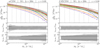 |
Fig. 4 B-spline decomposition of the HMF for SO haloes with ∆ = 200c at z = 0 in wCDM (left) and f(R)CDM (right) cosmologies. Top panel: measured HMF from the simulations (data points), with the corresponding errors bars (not always visible), and B-spline function fits (dashed lines). Each colour corresponds to a different training model. For visual clarity, only the models from the first slice of the quasi-PLHS are displayed (i.e. 16 models). The dashed vertical lines indicate the location of the B-spline knots. Middle panel: distribution of the fit residuals normalized by the noise in the simulation data. The dark and light shaded areas mark the 68.2% and 95.4% confidence intervals, respectively. The dashed lines indicate the ±1 and ±2σ levels. Bottom panel: distribution of the fit residuals normalized by the simulation data (i.e. the relative errors). The dark and light shaded areas mark the 68.2% and 95.4% confidence intervals, respectively. The shaded region corresponds to the ±1% level, along the y-axis the scaling is linear within the 1% region and logarithmic outside. The uncertainties on the B-spline fits are dominated by the simulation noise, except in the wCDM case at small masses, where they saturate at the ~0.5% level. |
4 Validation, tests, and comparisons
4.1 Validation with the leave-one-out method
The leave-one-out test consists in leaving a single model out of the emulator training set, and then comparing the predictions of the emulator to the simulation data of the left-out model. This is repeated for each model in the emulator training set, thus providing an estimation of the emulator accuracy across the whole parameter space.
It is worth noting that this is a quite stringent test. Firstly, uncertainties are tested across the sampled parameter space, including the edges. Secondly, after removing the tested model, the training set is incomplete and by design the left-out model is far from the other training points. Hence, if the emulator provides a good description of the left-out model, that is definitely an indication of robustness. Of course, the final emulator is trained using all the models, which results in smaller emulation errors. Nevertheless, this leave-one-out test provides a useful conservative estimate of the HMF emulation accuracy.
In Fig. 5, we plot the results of the leave-one-out test for the SO HMF with ∆ = 200c, and different redshifts, in the case of the wCDM and f(R)CDM models. In particular, we show the 68.2% and 95.4% confidence intervals of the distribution of relative errors. We find that the half width of the 68.2% interval is approximately described by a function of the form max {ϵ0, ϵ0 ⋅ (Mh/Mt)α. In wCDM, at z = 0, we find ϵ0 ≃ 1.5%, Mt ≃ 2·⋅ 1014 h−1M⊙ and α ≃ 0.9, up to the maximum halo mass of Mh ≃ 1015 h−1M⊙. As already shown in Fig. 3, the emulator range decreases at higher redshifts. As expected, the emulation accuracy at a given halo mass decreases with redshift. In the case of f(R)CDM we find at z = 0: ϵ0 ≃ 4%, M, ≃ 6 ⋅ 1013 h−1 M⊙ and α ≃ 0.4. Given the smaller number of f(R)CDM realizations per cosmological model, it is not surprising that the emulation accuracy is worse than in the wCDM case.
Figure 5 also shows the 1σ errors of the simulation data averaged over all cosmological models. At large masses, it follows the 68.2% confidence level of the relative errors from the leave-one-out test. We can conclude that in the high mass regime, the accuracy of the emulator is limited by the statistical noise in the training data. Increasing the accuracy of the emulator in this regime requires higher volume simulations or a larger number of realizations per cosmological model.
In order to validate the emulator error estimated by the emulator itself, we compare it to the error computed by the leave-one-out test. We find a good statistical agreement between both errors in the low mass end of the HMF. However, the emulator tends to overestimate the emulation accuracy in the high mass end. We multiplied the standard deviation predicted by the GPs by fixed factors, such that the distribution of leave-one-out errors normalized by the emulator estimated errors is close to a unit-variance normal distribution. This kind of technique to correct the error predicted by the emulator itself has already been used by Bocquet et al. (2020). We give in Fig. 5 the corrected 1σ emulation error, as estimated by the emulator itself, and averaged over all cosmological models. It can be seen that this error is in good agreement with the 68.2% confidence level of the leave-one-out errors for all masses and redshifts, which serves as a validation of the uncertainty predicted by the emulator. It means that the emulator is able to estimate its own accuracy, enabling users to account for (often overlooked) theoretical error bars during the cosmological inference process. In particular, the errors in the low mass end of the HMF are dominated by the interpolation between cosmological models and not the noise in the simulation data. Improving the emulator accuracy at low masses would require a higher number of training models or a more efficient emulation procedure. To conclude, the e-MANTIS emulator predicts the HMF at the few percent level over a wide range of masses and redshifts in f(R)CDM and wCDM cosmologies.
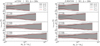 |
Fig. 5 Results of the leave-one-out test for the wCDM (left) and f(R)CDM (right) cosmologies, for multiple redshifts, and in the case of the SO HMF with ∆ = 200c. One model is excluded from the emulator training set, the corresponding predictions are compared to the simulation measurements of this model. The procedure is repeated for each of the 80 training models. The light and dark shaded areas mark the 68.2% and 95.4% confidence intervals of the resulting distribution of relative errors. The black dashed line gives the 1σ error from the simulation measurements, averaged over all cosmological models. The red dashed line indicates the 1σ emulation error estimated by the emulator itself, averaged over all cosmological models. In the left plot, the y-axis scaling is linear within the ±2% region and logarithmic outside. In the right plot, the y-axis scaling is linear within the ±5% region and logarithmic outside. |
4.2 Test with other N-body simulations
4.2.1 Test with e-MANTIS reference simulations
To test the predictive power of the HMF emulator, we compare its predictions to the set of simulations for the reference cosmological models P18, w12, and F5 presented in Sect. 2.5. The P18 and w12 cosmological models are chosen to be within 2σ of the cosmological parameters inferred from the 2018 analysis of Planck CMB data (Planck Collaboration VI 2020). The F5 model represents a significant deviation from ΛCDM, while being compatible with recent cluster abundance constraints (Artis et al. 2024). These models allow us to gauge the efficiency of the emulator in cosmologies which at the time of writing are considered realistic. These simulations use the L328_M10 box, and have 384 independent realizations for P18 and 64 realizations for w12 and F5. As these data were not used to train the emulator, they provide an ideal reference to which we can compare the predictions of the emulator.
In Fig. 6, we plot the HMF predicted by the emulator against that measured from the L328_M10_P18 simulation, at z = 0 and z = 1, and for the different halo mass definition. For this comparison, we use e-MANTIS without the low mass end resolution correction (see Sect. 3.2) in order to match the M10 mass resolution of the L328_M10_P18 simulation. In the top panels, we can see that there is a good agreement between the emulated HMFs and the simulation data, for all the halo definitions supported by the emulator. The bottom panels show the relative difference between the measured HMF and the predicted one, with the shaded area indicating the overall uncertainty estimated by adding in quadrature the error of the estimated HMF from the reference simulations (assumed to be Poisson noise) and the emulator uncertainty. We find such uncertainties to be dominated by the Poisson error, which is related to the number of halos in each mass bin. In particular, we can see that the relative difference between the measured HMF and the predicted one remains at the 1% level across the bulk of the mass interval, for the different halo mass definition. It increases up to the ~5% level only at the high-mass end, and with a scatter dominated by the Poisson noise, that is due to the reduced number of halos in the highest mass bins.
In Fig. 7, we compare the HMF predicted by the emulator against the HMF measured from the L328_M10_wl2 and L328_M10_F5 simulations, at z = 0. More specifically, in the top panels we show the ratio of the HMF with respect to that of the L328_M10_P18 simulation, while in the bottom panels we show the relative difference between the simulations measurements and the emulator predictions. Once again, there is a good agreement between the predictions of the HMF emulator and the HMFs from simulations. In the wl2 case, the differences are within the 1% level across the bulk of the mass interval, with larger errors occurring only in the highest mass bins due to Poisson noise. We obtain similar results for the F5 case, with differences at the 2% level over most of the mass interval. In both cases, the differences are within the expected combined uncertainties from the emulator and the shot-noise from the simulation data. The fact that the uncertainties estimated from the F5 analysis are slightly larger than the wl2 case is consistent with the fact that in the former case, the training set contains a factor 8 fewer simulations per cosmological model. Indeed, as explained in Sect. 4.1, the emulator error in f(R)CDM is a bit larger than in wCDM.
Overall, we find the emulator to be in good agreement with the simulation set for the reference P18, F5, and w12 cosmological models. In particular, there is a few per cent level agreement over a wide range of halo masses and for multiple halo definitions. At large masses, the differences grow due to the statistical noise both in the reference simulation data and in the emulator training set. In any case, the differences between the emulator predictions and the simulation data remain within the expected error bars.
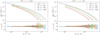 |
Fig. 6 Comparison of the emulator HMF predictions to the L328_M10_P18 simulation at z = 0 (left) and z = 1 (right). Top panels: HMFs measured from the simulation (solid circles) and emulator predictions (dashed lines) without resolution correction, such as to consistently match the resolution of the L328_M10_P18 simulation. The different colours correspond to the different halo mass definitions. The error bars correspond to the HMF simulation measurement errors, while the shaded area around the lines correspond to the uncertainties of HMF emulator predictions (not visible due to the small level of uncertainty). Bottom panels: relative difference between the simulation measurements and the emulator predictions. The shaded area correspond to the Iσ confidence interval combining both the simulation noise and the emulator accuracy. There is a good agreement with differences of the order of a few percent level, and within the expected error bars. |
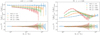 |
Fig. 7 Comparison of the emulator HMF predictions at z = 0 in wCDM (left) and f(R)CDM (right) to the HMF of L328_M10_wl2 (left) and L328_M10_F5 (right). The HMFs are normalized by the L328_M10_P18 simulation data. Top panels: ratio of the wCDM (left) HMF or f(R)CDM (right) HMF to the ΛCDM one measured from the simulation (solid circles) and from emulator predictions (dashed lines). The error bars correspond to the HMF simulation measurement errors (not always visible for small errors), while the shaded area around the lines correspond to the uncertainties of HMF emulator predictions. Bottom panels: relative difference between the HMF simulation measurements and the emulator predictions. The shaded area correspond to the 1σ confidence interval combining both the simulation noise and the emulator accuracy. There is a good agreement with differences of the order of a few percent level, and within the expected error bars. |
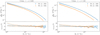 |
Fig. 8 Comparison of the emulator HMF predictions to that estimated from the Uchuu simulation, at z = 0 (left) and z = 1.03 (right). Top panels: HMF from the simulation (solid circles) and emulator predictions with (solid lines) and without (dashed lines) resolution correction. The noise in the simulation measurements and the emulator predictions are given as error bars and a shaded area respectively around the corresponding lines (not always visible for small errors). The Uchuu haloes have been detected with the Rockstar halo finder (Behroozi et al. 2013). Bottom panels: relative difference between the simulation measurements and the emulator predictions with (solid lines) and without (dashed lines) resolution correction. The shaded areas mark the 1σ confidence interval, combining both the simulation data noise and the emulator accuracy. |
4.2.2 Test with publicly available N-body simulations
We now present a comparison of the HMF predicted by the e-MANTIS emulator against numerical estimates from publicly available N-body simulations. First, we use the halo catalogues from the Uchuu simulation6 (Ishiyama et al. 2021). These allow us to compare the HMF prediction of the emulator to a simulation which has larger volume, (2 h−1Gpc)3, and a better mass resolution mpart = 3.28 ⋅ 108/z−1M⊙, than those of the e-MANTIS training set. Moreover, the Uchuu simulation has been run using a different numerical N-body code from the one used in this work, GreeM (Ishiyama et al. 2009, 2012); similarly, the halo catalogues have been generated using a different halo finder, Rockstar (Behroozi et al. 2013). All these differences allow us to test resolution effects as well as the consistency of the results with respect to the different numerical codes used to perform and analyse the e-MANTIS simulations. The Uchuu simulation uses a flat ΛCDM cosmological model compatible with Planck Collaboration XIII (2016): Ωm = 0.3089, h = 0.6774,  , Ωb = 0.0486, ns = 0.9667.
We estimate the Uchuu HMFs at two overdensity contrasts, ∆ = 200c and ∆ = 500c respectively. We do not include the case of ∆ = 1000c in this comparison, since the necessary Uchuu data is not available. In Fig. 8, we compare the HMF predicted by the e-MANTIS emulator to the Uchuu HMFs, with and without the low mass end resolution correction presented in Sect. 3.2, both at z = 0 and z = 1.03. We can see that including the correction significantly reduces the relative difference between the emulator predictions and the simulation measurements from ˜20% to ˜5% at the low mass end (Mh ≃ 1013 h−1M⊙) and at z = 0, showing that the emulator predictions are in agreement with the Uchuu HMFs at the few percent level, despite the many differences between the simulation settings. We attribute the remaining differences to the different halo finders (Knebe et al. 2011) and N-body codes. We note that the discrepancies in the low mass end are smaller at z = 1.03. In the high mass end, the differences are within the expected error bars from the emulator uncertainty combined with the simulation shot-noise. We find similar results for all the other redshifts in the range 0<z< 1.5.
To benchmark the predictive power of the emulator for cosmologies alternative to ΛCDM, we consider two additional simulation suites, the wCDM RayGalGroupSims runs (Rasera et al. 2022), hereafter RayGal, and the f(R) gravity ELEPHANT runs (Cautun et al. 2018; Gupta et al. 2022). Both these suites adopt numerical settings similar to those of the e-MANTIS simulation training set. As an example, both suites were run using the code RAMSES. Furthermore, the ELEPHANT suite also uses the ECOSMOG implementation (Li et al. 2012; Bose et al. 2017) of the Hu & Sawicki (2007) f(R) modified gravity model. Here we focus on the HMF boost, that is, the ratio of the HMF in an alternative cosmology with respect to ΛCDM. Different systematic errors, such as resolution effects or differences in the halofinders, largely cancel out using this boost. We discuss some of these systematic effects in more details in Sect. 4.3.1. The aim of the present test is to focus on the cosmological dependence with respect to the alternative parameters.
The RayGal runs consist of two large volume simulations of (2625/h−1Mpc)3 of a flat ΛCDM model and a flat ωCDM scenario with constant equation of state w = −1.2. The cosmological parameters of these simulations were chosen to be consistent with the results of the WMAP-7 year (Komatsu et al. 2011) and Planck (Planck Collaboration VI 2020) data of the CMB anisotropy power spectra. In particular, the ΛCDM run assumes Ωm = 0.25733 and  , while the wCDM run assumes Ωm = 0.27508 and
  . The remaining cosmological parameters are fixed to Ωb = 0.04356, h = 0.72, ns = 0963, and Ωr ≃ 0.00008 respectively. In both simulations, the dark matter density field is traced by 40963 N-body particles, leading to the two simulations having slightly different mass resolution, with mpart = 1.88 ⋅ 1010 h−1M⊙ in the case of the ΛCDM run and mpart = 2.01 ⋅ 1010 h−1M⊙ for the ωCDM case.
It is worth noticing that for each cosmological model in the wCDM emulator training dataset, the sample of small volume simulations, L328_M10_wcdm, represent a total effective volume equivalent to an eighth of the full RayGal volume for each training cosmological model, with similar mass resolution (not considering the resolution correction presented in Sect. 3.2). We note that the RayGal simulations used a triangular shaped cloud (TSC) interpolation in the dynamical solver, while the e-MANTIS training set uses a CIC interpolation. This difference in the interpolation scheme results in a slightly different effective resolution at equal N-body particle mass. The sample of larger volume simulations, L656_M11_wcdm, covers a volume equivalent to the simulation box of the RayGal runs for each cosmological model, with lower mass resolution.
In Fig. 9, we plot the ratio of the HMF estimated from the wCDM RayGal run to the HMF estimated from the ΛCDM simulation and compare these estimates to the same ratio predicted by e-MANTIS, both at z = 0 and z = 1. We find that the predictions are accurate to the level of a few percent at the low mass end, and reach a maximum difference with respect to the simulation data of ~10% in the largest mass bins. At all masses, the relative difference is generally consistent with the uncertainty of the emulator and the Poisson noise in the simulation data. Similar results are found at other redshifts in the range 0 < z < 1.5. We may notice that the trend shown in Fig. 9 differs from that in Fig. 7. This is essentially due to the differences in the values of  and ΩM between the two RayGal runs, whereas in Fig. 7 the difference is solely due to the dark energy equation of state parameter.
The ELEPHANT runs evolve 10243 JV-body particles in a volume of (1024 /z_1Mpc)3, with a particle mass of mpart = 7.798 ⋅ 1010 h−1M⊙. In addition to a ΛCDM model, there are simulations for three different f(R) gravity models:  , , and
  . The other cosmological parameters are fixed to the best-fit values from the WMAP-9 year analysis (Hinshaw et al. 2013):
  , h = 0.697, ΩB = 0.046, and ns = 0.971. There are 2 independent realizations in F4 and 5 independent realizations in ΛCDM, F5, and F6 (see Gupta et al. 2022). These simulations are run using the ECOSMOG implementation of the Hu & Sawicki (2007) model. The dark matter halo catalogues and HMF measurements have been obtained by Gupta et al. (2022) using the Rockstar halo finder.
In Fig. 10, we show the HMF ratio in each f(R) model with respect to ΛCDM, as measured from the ELEPHANT simulations and as predicted by e-MANTIS, both at z = 0 and z = 1. In the case of F6 at z = 0, the agreement is within the expected errors from the emulator and the simulation Poisson noise. At z = 1, this is also true for masses Mh ≲ 1014 h−1 M⊙. For F5, the differences are within the expected error bars at z = 1, while at z = 0 they are slightly larger, but remain at the ~5% level for the whole mass range. For F4, the differences are at the ~5% level for masses Mh≲3 ⋅ 1014 h−1M⊙ and M⊙ ≲ 5 ⋅ 1013 h−1M⊙, for z = 0 and z = 1, respectively. These differences might once again be due to the different halo finders, however a more dedicated study is required to reach a conclusion. Overall, we find that the predictions of e-MANTIS for the HMF boost in f(R) gravity are in good agreement with the data from the ELEPHANT simulations at the ~5% level, for most masses, redshifts, and models, while larger discrepancies are present in some cases, such as for high redshifts together with large masses or large values of 
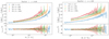 |
Fig. 9 Comparison of the e-MANTIS predictions for the ratio of the HMFs from the two RayGal simulations for different halo definitions at z = 0 (left) and z = 1 (right). Both RayGal simulations differ not only in the value of w, but also in terms of Ωm and |

4.3 Comparison to existing HMF predictions
In the previous section, we have validated the e-MANTIS HMF emulator from group-masses to cluster-masses and redshifts z < 1.5, using both internal and external simulations in ΛCDM, wCDM, and f(R)CDM cosmologies. As the goal of e-MANTIS is to provide fast (~10 ms) predictions of the HMF (as well as other observables of the non-linear clustering of matter) for various applications requiring speed and accuracy, such as MCMC cosmological inference, it is of interest to compare its predictions to that of other emulators as well as those from analytically calibrated models of the HMF. For this purpose, we first compare predictions for the ΛCDM cosmology, and then discuss the case of wCDM and f(R)CDM models. More specifically, we start by a comparison of the full HMF for a fixed cosmology in ΛCDM. They aim is to study the systematic differences that exist between different predictions for a fixed cosmological model. Then, we turn to the study of the HMF boost in wCDM and f(R)CDM models. This time, the objective is to focus on the cosmological dependence. As already stated earlier, several systematic errors cancel out in the boost, which allows a more precise study of the cosmological dependence.
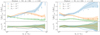 |
Fig. 10 Comparison between the e-MANTIS predictions and the measurements from the ELEPHANT simulations (Cautun et al. 2018; Gupta et al. 2022) for SO haloes with Δ = 200c at z = 0 (left) and z = 1 (right). Top panels: measured HMF boost from the simulations (solid circles) and predictions from the emulator (dashed lines). The noise in the simulation measurements and the emulator predictions are given as error bars and a shaded area respectively around the corresponding lines (not always visible for small errors). Bottom panels: relative difference between the simulation measurements and the emulator predictions. The shaded areas mark the 1σ confidence interval, combining both the simulation data noise and the emulator accuracy. |
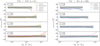 |
Fig. 11 Relative difference between different HMF predictions from other works found in the literature and e-MANTIS, for the reference P18 cosmology and at different redshifts. Solid lines correspond to predictions from fits to simulations, and dashed lines to emulators. Left: FoF haloes with b = 0.2. Right: SO haloes with Δ = 200c. The light and dark shaded areas mark the ±5% and ±10% levels, respectively. |
4.3.1 ΛCDM
In Fig. 11, we plot the relative difference between several popular predictions (namely Tinker et al. 2008; Crocce et al. 2010; Bhattacharya et al. 2011; Courtin et al. 2011; Angulo et al. 2012; Watson et al. 2013; Despali et al. 2016; Bocquet et al. 2016), as implemented in COLOSSUS (Diemer 2018), and the e-MANTIS HMF at z = 0, z = 0.5, z = 1, and z = 1.5 for the P18 reference cosmology. We consider two common choices of halo definition: FoF haloes with a linking-length b = 0.2 widely used in the N-body simulation community, and SO haloes with an overdensity threshold Δ = 200c widely used in the galaxy cluster community. We also compare our prediction to that of Mira-Titan emulator (Bocquet et al. 2020). While we only consider one external emulator in our comparison, we note that other HMF emulators are available in the literature, such as Dark Emulator (Nishimichi et al. 2019) and Aemulus (McClintock et al. 2019). However, to the best of our knowledge, these are restricted to other mass definitions, such as 200 times the mean background density. Overall, it is important to stress that all the models agree with the e-MANTIS predictions, with relative deviations of less than 10% over a wide range of redshifts and masses. The deviations only exceed the 10% level for some predictions at the high-mass end, where the statistical noise related to the limited simulation volume is expected to be large due to the steepness of the mass function. In this regime, the estimated HMF is also very sensitive to initial condition truncation and discreteness errors, finite mass resolution effects, and other systematic effects.
In the following, we discuss the comparison with the different predictions case by case. Notice that as our emulator provides predictions with an accuracy better than ~5% when confronted to external N-body simulations, then differences of the various HMF calibrated parametrizations will be indicative of their accuracy in reproducing the simulation results:
Crocce et al. (2010) FoF mass function: the agreement is at the 5% level for Mh ≲ 1015 h−1 M⊙ at z = 0, while it degrades to the 7% for Mh ≲ 3 · 1014 h−1 M⊙ at z = 1. In contrast, the deviation with respect to the prediction from e-MANTIS increases up to the 20% level at the very high mass-end. We do not show the comparison at redshifts z > 1, since these are outside the limit of validity of their fitting formula.
Bhattacharya et al. (2011) FoF mass function: the agreement is at the 3% level from z = 0 to z = 1 over a wide range of masses (up to 1015 h−1 M⊙ at z = 0 and 3 · 1014 h−1 M⊙ at z = 1). At z = 1.5 the fit is ~5% below our prediction.
Courtin et al. (2011) FoF mass function: the agreement is at the 5% level up to 3 · 1014 h−1 M⊙ at z = 0. The difference increases up 10 – 20% between 9 · 1014 h−1 M⊙ and 1.3 · 1015 h−1 M⊙, while the fit is not valid beyond this mass scale. We only show the comparison at z = 0, as for higher redshifts it would require a conversion of the FoF halo masses that is beyond the scope of this analysis.
Angulo et al. (2012) FoF mass function: the agreement is between 2 and 3% level up to 1.5 · 1015 h−1 M⊙ at z = 0, while no fitting formula is provided at higher redshift.
Watson et al. (2013) FoF mass function: at z = 0 the HMF prediction is below that of our emulator at ~ 10% level in the low-mass range and improves to ~5% up to 1015 h−1 M⊙. At z = 0.5 the agreement is at 3% level up to 9 · 1014 h−1 M⊙ and similarly for z = 1 up 2 · 1014 h−1 M⊙. At z = 1.5 the agreement is ~3% at the low-mass end and degrades beyond 10% level at the high-mass end with steep slope probably related to the redshift-independence of the fitting parameters.
Tinker et al. (2008) SO mass function: the agreement with the e-MANTIS prediction at z = 0 is on average at 1% level across the full mass range. At higher redshifts, the fit falls progressively below the emulator. For instance, at z = 0.5 it drops on average at ~2%, at z = 1 is of the order of ~5%, while at z = 1.5 the difference amounts on average to ~12% (ranging from 7% near 1013 h−1 M⊙ to 20% near 1.5 · 1014 h−1 M⊙). Recent analyses of numerical simulations as well as the testing of emulators have shown that the Tinker et al. (2008) fit is only accurate at low redshifts. As an example, the Mira-Titan emulator is 10% above the fit, as we will discuss below. Moreover, McClintock et al. (2019) have shown that while the precision of the fit is of order ~5% at z = 0, errors can reach very large value at z = 2. Nishimichi et al. (2019) has also shown very precisely that at z = 1.48 their simulations predict a larger mass function by 13% near 1013 h−1 M⊙ to 18% near 1014 h−1 M⊙, which is compatible with our finding given that the mass definition is slightly different at this redshift.
Despali et al. (2016) SO mass function: the agreement at z = 0 is at the 2% level up to 2 · 1014 h−1 M⊙, while at larger masses the fit strongly deviates from the emulator prediction, reaching a 25% discrepancy at 1015 h−1 M⊙. This very steep increase is likely due to the more rigid functional form of the fitting function, making it difficult to accurately capture the shape of the HMF at large masses. At z = 0.5 the agreement degrades to 5% level up 3.5 · 1014 h−1 M⊙ and increases at larger masses up to ≈ 10% level. We can see that the agreement further degrade at the ~10% level at z = 1 and the ~15% level at z = 1.5. Deviations from Despali et al. (2016) have already been found in the literature (see e.g. Shirasaki et al. 2021).
Bocquet et al. (2016) SO mass function: at z = 0 the agreement is at the ~8% level in the low mass end (see the next item for a more detailed discussion), and improves up to ~3% in the high mass end. At higher redshifts, the COLOSSUS implementation of this fit gives predictions that are not in agreement with the results presented in Bocquet et al. (2016), with differences of up to 20 – 30%. Therefore, we suspect a bug in the implementation and exclude redshifts z > 0 from this comparison.
Bocquet et al. (2019) SO mass function (Mira-Titan emulator): the agreement at z = 0 is at the ~8% level in the low mass range Mh < 1014 h−1 M⊙, it improves up to ~3% in the mass interval 1014 ≲ Mh [h−1 M⊙] ≲ 6 · 1014 and then degrades up to 10% level at higher masses. We find the same level of agreement at z = 0.5,1 and 1.5, though in the latter case we find a deviation exceeding the 10% level at the very high-mass end. It is important to stress that the redshift evolution is in much better agreement than that found in the case of the Tinker et al. (2008) and Despali et al. (2016) fits. The ~8% discrepancy at small masses is consistent with the results of the comparison performed in Bocquet et al. (2019) between the z = 0 Tinker et al. (2008) mass function, the rescaled Aemulus mass function and the Mira-Titan mass function, where the authors have found that Aemulus and Tinker et al. (2008) mass functions are in good agreement, while the Mira-Titan is 8% below. This is not an error of Mira-Titan, but the consequence of having a different halo mass definition. In fact, while our emulator is calibrated on SO halo catalogues, the Mira-Titan uses a mixture of FoF detection with SO-like masses. This also accounts for the difference at low mass between e-MANTIS and the fit from Bocquet et al. (2016). Moreover, differently from the e-MANTIS emulator, no mass resolution correction has been accounted in their training data.
To conclude the comparison of the HMF predicted by parametric models and the e-MANTIS predictions in the ΛCDM case, we found an overall good agreement at z = 0 while discrepancies become more important at higher redshifts. While some fits are specialized to particular halo definitions (e.g. Bhattacharya et al. 2011; Angulo et al. 2012), others are very flexible (e.g. Tinker et al. 2008; Despali et al. 2016), which comes at the cost of precision for a given mass definition. The comparison with the predictions of the Mira-Titan emulator show differences ~3 – 10%. These primarily result from the fact that e-MANTIS emulator for different overdensity thresholds has been calibrated using halo catalogues generated with a SO halo finder, while Mira-Titan relies on FoF halos with spherical masses at different overdensity thresholds. Moreover, e-MANTIS accounts for mass resolution effects on the predicted HMF.
4.3.2 wCDM & f(R)DM
We now compare the predictions of the calibrated parametrizations of the HMF as well as those from other emulators to those of the e-MANTIS emulator in the case of wCDM and f (R)CDM cosmologies respectively. These are shown in Figs. 12, 13 and 14, where we plot the boost, that is the ratio of the HMF predicted in the non-standard cosmological scenario with respect to the ΛCDM case, as well as the corresponding relative difference with respect to e-MANTIS.
In Fig. 12, we show the HMF boost for the wCDM scenario as predicted by e-MANTIS against other HMF predictions. In particular, we consider multiple values of the dark energy equation of state, ranging from w = −1.5 to w = −0.5, while the other cosmological parameters are fixed to the values of the reference P18 cosmological model. We focus on two different halo definitions: SO haloes with Δ = 200c and FoF haloes with b = 0.2. At z = 0, the parametric fits fail to capture the dependence of the boost on w. This is because their predictions only rely on the dependence of the HMF on the linear matter power spectrum, which at z = 0 is identical for all values of w, since we have fixed Ωm and  . However, deviations from a universal HMF are expected, since the linear growth rate ƒ = d ln D+ /d ln a (where D+ is the linear growth factor) does depend on the equation of state of dark energy w (Courtin et al. 2011; Ondaro-Mallea et al. 2022). Hence, in the case of the parametric fits, this translates into an error on the predicted HMF boost of up to ~5% for FoF haloes, and up to ~20 for SO haloes. We can see that this is not the case of the Mira-Titan emulator, for which predictions are in very good agreement with e-MANTIS at all redshifts, with only deviations of a few per cent at the largest masses. Indeed, the emulators are more efficient at capturing the impact of the dark energy equation of state on the HMF. Nevertheless, given the smaller range of values of w covered by Mira-Titan we were not able to compare the HMF predictions for w = −0.5 and w = −1.5. It is worth noticing that at z > 0 the parametric fits perform better than at z = 0, since they capture part of the cos-mological dependence of the HMF caused by variations in the linear matter power spectrum.
In Fig. 13, we plot the relative difference between the various predictions of the wCDM boost with respect to e-MANTIS at different redshifts, again for FoF haloes with b = 0.2 and SO haloes with ∆ = 200c. As the trends are similar for all wCDM models, and to improve the readability of the graph, we focus on a single dark energy model with w = −1.3. At z = 0, we find ~2 – 4% errors in the case of FoF haloes, and 3 – 15% errors in the case of SO one. At z > 0, in both the FoF and SO cases, the resulting error is of order ±2 – 3% for most of the mass range, while at high masses it can reach the 5% level for FoF haloes and the 10% level for SO haloes.
We now turn to the f (R)CDM case. Analytical predictions of the mass function in modified gravity is a notoriously difficult problem. Using standard parametric fits, such as those previously discussed, with modified linear power spectra and with a fixed critical density δc from the spherical collapse model, fails to describe the HMF from simulations of modified gravity models. Accounting for the screening mechanism is highly non-trivial. Many attempts exist to predict the mass function in f (R) gravity using various formulation of the excursion set theory, with a critical density threshold that can depend on mass and also the environment (Li & Efstathiou 2012; Lam & Li 2012; Lombriser et al. 2013; Kopp et al. 2013; Cataneo et al. 2015; Shi et al. 2015; Cataneo et al. 2016; Achitouv et al. 2016; von Braun-Bates & Devriendt 2018; Gupta et al. 2022). The implementation of all these complex models is far beyond the scope of the work presented here. Hence, we have opted to compare the predictions for the SO mass function boost at z = 0 from the e-MANTIS emulator to the predictions of the f (R) gravity emulator built by Ruan et al. (2022). This emulator is based on the N-body simulation suite from Arnold et al. (2022), whose simulations have been run with a modified gravity version of the AREPO code (Springel 2010; Arnold & Li 2019). It is complementary to our emulator since it targets the masses range 1012 < Mh[h−1 M⊙] < 1014, while we focus on the mass range of groups and clusters 1013 < Mh[h−1 M⊙] < 1015.
In Fig. 14, we plot the boost predicted by the two emulators for f (R)CDM models with  , 10−5.5 and 10−5 at z = 0, where we have fixed the other cosmological parameter values to those of the ELEPHANT simulations (Cautun et al. 2018). We can see that the shape of the boost is similar for all
  values. In the common range of masses, there is an excellent agreement for the HMF boost predicted by the two emulators at the 2% level for F6 and F5.5, while deviations are smaller than 5% for F5. Given that the emulators have been trained on different simulation datasets, using different N-body and halo finder codes, the 5% difference is a good achievement. To conclude, in terms of the HMF boost, the emulators are compatible at the few percent level and they span a complementary mass range.
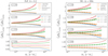 |
Fig. 12 Ratio of the HMF in wCDM with respect to ΛCDM for different values of w and at different redshifts, as predicted by e-MANTIS as well as multiple HMF predictions from other works. Left: FoF haloes with b = 0.2. Right: SO haloes with Δ = 200c. Only the dedicated emulators are able to fully capture the cosmological and redshift dependence of the HMF. |
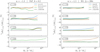 |
Fig. 13 Relative difference between different existing predictions and e-MANTIS, for the ratio of the HMF in wCDM with respect to ΛCDM. We consider a wCDM model with w = −1.3. Left: FoF haloes with b = 0.2. Right: SO haloes with Δ = 200c. |
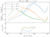 |
Fig. 14 Comparison between the e-MANTIS predictions and those of the emulator from Ruan et al. (2023). Top panel: ratio of the HMF in f (R) gravity with respect to ΛCDM for different values of |

5 Conclusions
We have presented a novel emulator of the HMF implemented in the framework of the e-MANTIS emulator, originally developed to provide accurate predictions of the non-linear matter power spectrum of f (R)CDM cosmologies (Sáez-Casares et al. 2023). Not only have we implemented a new functionality, we have also extended the cosmological parameter space for which e-MANTIS can provide accurate predictions, and which now include the case of wCDM models. For this purpose, we have carried out a large suite of N-body simulations using a Latin hyper cube sampling the six-dimensional parameter space consisting of the standard cosmological parameters Ωm, σ8, h, ns, and Ωb and  for f (R)CDM, and w for wCDM models. We considered a large range for the non-standard parameters:
 ![Mathematical equation: ${f_{{R_0}}} \in [ - 7, - 4]$](/articles/aa/full_html/2024/11/aa50193-24/aa50193-24-eq46.png) and w ∊ [−1.5, −0.5]. In particular, for each model the simulations span 80 different combinations for the parameters with a different simulation volume, mass resolution, and random phase for the initial conditions. The total number of simulations in this extended e-MANTIS simulation suite exceeds 10 000.
and w ∊ [−1.5, −0.5]. In particular, for each model the simulations span 80 different combinations for the parameters with a different simulation volume, mass resolution, and random phase for the initial conditions. The total number of simulations in this extended e-MANTIS simulation suite exceeds 10 000.
We have generated halo catalogues for each of the simulations in the suite using two different halo finders. Hence, contrary to other emulators presented in the literature (see e.g. McClintock et al. 2019; Nishimichi et al. 2019; Bocquet et al. 2020), the e-MANTIS emulator of the HMF is capable of providing accurate and fast predictions in the case of FoF halos with linking length b = 0.2 as well as SO halos with overdensity values compatible with those of observable mass definitions of galaxy clusters ∆ = 200c, 500c, 1000c. In the latter case, we have detected SO halos with a detection threshold of ∆ = 200c and then computed the halo masses at ∆ = 500c and 1000c from the mass profile.
We have built HMF training datasets using a B-spline basis decomposition for the HMFs estimated from the simulation suite. This is particularly important if one aims to obtain accurate predictions for the HMF for modified gravity models, since traditional fitting formulae do not perform as well as in standard GR-based scenarios (see e.g. Gupta et al. 2022). We do indeed find that the B-spline decomposition is able to capture the shape of the HMFs with a per-cent level accuracy at low masses, while at large masses the performance of the fit is only limited by the statistical noise of the simulation data. We used a Gaussian process regression to emulate the cosmological dependence of the B-spline coefficients, while we used a linear interpolation of the logarithm of the HMF as a function of scale factor to capture the redshift dependence. The final emulator is able to predict the HMF for the different halo definitions described above in the redshift range 0 ≤ z ≤ 1.5 and over the range of masses 1013 ≲ Mh[h−1 M⊙] ≲ 1015 for which the emulator has been designed, both for wCDM and f (R)CDM models.
We have performed a thorough analysis to assess the accuracy of the emulator predictions. In particular, the results of the leave-one-out tests show that the emulator achieves an accuracy of a few per cent in the low-mass end of the HMF, where the error budget is dominated by the emulation itself. In the higher-mass end, the emulation error is dominated by the statistical noise in the training HMF simulation data. Overall, the results indicate an accuracy better than a few per cent over a wide range of halo masses. As an example, the errors on the HMF prediction for SO halos at z = 0 in the case of wCDM models are at the ~1.5% level up to M200c = 2 · 1014 h−1 M⊙. The comparison with the HMF estimated from the large volume high-resolution Uchuu simulation shows an agreement better than 5% for all masses and redshifts considered, and this further validates the mass resolution correction that we applied to our training data. In terms of the cosmological dependence of the HMF boost, that is to say the ratio between the HMF in an alternative cosmology with respect to ΛCDM, we find an agreement better than 5% over a wide range of masses with the measurements from the simulations of RayGal, that is to say in wCDM, and Elephant, that is, in f (R)CDM.
This is a noticeable result, especially in the case of the Uchuu and Elephant simulations, which were carried out using different halo finders than those we have used for the e-MANTIS simulation suite. Moreover, the e-MANTIS emulator provides an estimate of its own errors, thus enabling the possibility to propagate such model prediction uncertainties in the cosmological parameter inference analysis. We have tested the predictions against those from existing fitting formula of the HMFs as well as publicly available emulators. We show that only emulators can account for departure from the universality of the HMF. Ignoring such deviations can lead to up to 25% errors on the SO mass function at the high-mass end. We find good agreement with the predictions for the Mira-Titan emulator in the wCDM case. The comparison with the HMF emulator for f (R)CDM models from Ruan et al. (2023), which targets the mass interval 1012 ≲ Mh[h−1 M⊙] ≲ 1014, shows an agreement better than 5%, in terms of the HMF boost, in the common mass range for different values of  .
.
It is worth noting that the e-MANTIS emulator is calibrated on dark-matter-only simulations and consequently does not include the effect of baryonic physics. The feedback caused by baryons on the matter distribution can have an impact on the HMF at the 10 – 20% level (Cui et al. 2012; Bocquet et al. 2016; Castro et al. 2021). Such effects need to be included in theoretical predictions of the HMF. However, hydrodynamical simulations including baryonic physics are computationally orders of magnitudes more expensive than dark-matter-only simulations. Consequently, building an emulator based on such simulations remains very challenging. Nevertheless, recent studies have shown that in the case of dynamical dark energy scenarios (which include the case of wCDM models), it is possible to disentangle the impact of baryons on the HMF from that of the cosmological model with a per-cent level accuracy (Pfeifer et al. 2020). Therefore, it should be possible to include the effect of baryons on the HMF as a post-processing step. Similarly, Arnold & Li (2019) have shown that the impact of baryons on the HMF in f (R) gravity can be estimated from hydrodynamical simulations of ΛCDM. Hence, as a first approximation, a ΛCDM baryonic correction to the HMF can also be applied to a dark-matter-only predictions for f (R)CDM models.
The calculation time of the HMF with the e-MANTIS emulator is of the order ~ 10 ms, while it combines the accuracy and possibility of exploring a wide range of cosmologies. Moreover, the emulator can be easily implemented in the standard MCMC likelihood analysis pipelines. As such, it provides a useful tool to constrain alternative dark energy models using galaxy cluster abundance measurements from the new generation of galaxy cluster surveys.
Acknowledgements
This project has benefited from computational time and data storage resources allocated by GENCI (Grand Équipement National de Calcul Intensif) at TGCC (Très Grand Centre de Calcul) for the projects 2021-A0110402287, 2022-A0130402287 and 2023-A0150402287 on the Joliot Curie supercomputer’s ROME and SKYLAKE partitions. We thank the Euclid Consortium for the “Sponsor PhD Grant” of ISC. YR acknowledges support from ANR (Agence Nationale de la Recherche) ProGraceRay (ANR-23-CE31-0010). We thank Baojiu Li for sharing the ECOSMOG simulation code. We thank Razi Sheikholeslami for sharing the PLHS MATLAB code, which served as validation for our own Python implementation. We thank Suhani Gupta for sharing the Elephant HMF data used in Figure 10. We are also grateful to Cheng-Zong Ruan et Baojiu Li for providing the predictions of the boost of f (R)CDM models with the emulator presented in Ruan et al. (2022). The plots presented in this paper were produced with the Matplotlib (Hunter 2007) package. A significant amount of the numerical computations were carried out using the SciPy (Virtanen et al. 2020), NumPy (Harris et al. 2020) and scikit-learn (Pedregosa et al. 2011) packages.
Appendix A Sampling of the cosmological parameter space
 |
Fig. A.1 Distribution of cosmological model parameter values of the wCDM and f (R)CDM emulators. The blue points correspond to the 80 training models of the emulators presented in this paper. The light grey points correspond to the remaining 176 models of the quasi-PLHS that may be used for a future extension of the simulation suite. Notice that the w and |

Appendix B Numerical convergence
In Sect. 3.2, we have presented a mass resolution correction for the emulator L328_M10 simulations using the higher resolution L328_M9_wcdm simulation set. This correction was used to upscale the low mass end of the emulator HMF training data from the M10 resolution to the M9 resolution. However, it is not guaranteed that the M9 simulations have fully converged for the mass range of interest. In order to test this, we used a set of simulations using a box-size of Lbox = 164.0625 h−1 Mpc and with different number of N-body particles: 2563, 5123, and 10243 corresponding to the resolutions M 10, M9, and M8 respectively. The initial conditions from the M10 and M9 simulations are degraded versions of the M8 initial conditions. These simulations use the P18 cosmological model. We computed the ratio of the M9 and M8 HMF to the M10 HMF. We estimated the corresponding errors using 43 spatial jackknife sub-volumes, in order to account for the correlation between the different simulations. These ratios are shown in Fig. B.1, along with the fitted correction used for the emulator training data, for SO haloes with ∆ = 200c at z = 1 and z = 0. We remind that the emulator only uses data for SO haloes with a number of particles larger than Npart,M10 = 300. We find that the in this mass range, the M9 HMF is in good agreement with the measurements from M8. We cannot see any statistically significant deviations from our correction at higher resolution. Therefore, the HMF from the M9 simulations has properly converged in the mass range of interest and no further resolution correction is required. We obtain the same conclusion for all the halo definitions and redshifts relevant for our emulator.
The correction computed in Sect. 3.2 has been obtained from wCDM simulations. We want to validate that it is still valid in the case of f (R) gravity. We use HMF measurements from simulations using the L164_M9 simulations box, for two different values of the  parameter:
  and
and  (F6). Figure B.1 shows that, in the case of SO haloes with ∆ = 200c, the HMF ratio measured from the F5 and F6 simulations is compatible the with correction fitted from the wCDM simulations. We find that this result holds for the other halo definitions and redshifts considered in this work. We can therefore safely apply such correction to the f(R)CDM emulator training data.
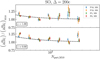 |
Fig. B.1 Ratio of the L164_M9 HMF, for the cosmological models P18, F5, and F6, and the L164_M8 HMF, for the model P18, with respect to the L164_M10 HMF, in the case of SO haloes with ∆ = 200c at z = 1 and z = 0. For visual clarity, the x coordinates have been slightly displaced. The dashed lines correspond to the fit performed in Sect. 3.2, which is used to correct the training data of the emulator from the L328_M10 simulations. We do not detect any statistically significant deviations from this fit, due to the effect of f (R) gravity or the higher M8 resolution. |
References
- Abbott, T. M. C., Aguena, M., Alarcon, A., et al. 2020, Phys. Rev. D, 102, 023509 [Google Scholar]
- Achitouv, I., Baldi, M., Puchwein, E., & Weller, J. 2016, Phys. Rev. D, 93, 103522 [NASA ADS] [CrossRef] [Google Scholar]
- Allen, S. W., Evrard, A. E., & Mantz, A. B. 2011, ARA&A, 49, 409 [Google Scholar]
- Amendola, L., Appleby, S., Avgoustidis, A., et al. 2018, Liv. Rev. Relativ., 21, 2 [NASA ADS] [CrossRef] [Google Scholar]
- Angulo, R. E., Springel, V., White, S. D. M., et al. 2012, MNRAS, 426, 2046 [NASA ADS] [CrossRef] [Google Scholar]
- Angulo, R. E., Zennaro, M., Contreras, S., et al. 2021, MNRAS, 507, 5869 [NASA ADS] [CrossRef] [Google Scholar]
- Arnold, C., & Li, B. 2019, MNRAS, 490, 2507 [NASA ADS] [CrossRef] [Google Scholar]
- Arnold, C., Li, B., Giblin, B., Harnois-Déraps, J., & Cai, Y.-C. 2022, MNRAS, 515, 4161 [CrossRef] [Google Scholar]
- Artis, E., Ghirardini, V., Bulbul, E., et al. 2024, A&A, 691, A301 [NASA ADS] [CrossRef] [EDP Sciences] [Google Scholar]
- Ba, S., Myers, W. R., & Brenneman, W. A. 2015, Technometrics, 57, 479 [CrossRef] [Google Scholar]
- Behroozi, P. S., Wechsler, R. H., & Wu, H.-Y. 2013, ApJ, 762, 109 [NASA ADS] [CrossRef] [Google Scholar]
- Bhattacharya, S., Heitmann, K., White, M., et al. 2011, ApJ, 732, 122 [NASA ADS] [CrossRef] [Google Scholar]
- Blot, L., Corasaniti, P. S., Alimi, J. M., Reverdy, V., & Rasera, Y. 2015, MNRAS, 446, 1756 [NASA ADS] [CrossRef] [Google Scholar]
- Blot, L., Corasaniti, P.-S., Rasera, Y., & Agarwal, S. 2021, MNRAS, 500, 2532 [Google Scholar]
- Bocquet, S., Saro, A., Dolag, K., & Mohr, J. J. 2016, MNRAS, 456, 2361 [Google Scholar]
- Bocquet, S., Dietrich, J. P., Schrabback, T., et al. 2019, ApJ, 878, 55 [Google Scholar]
- Bocquet, S., Heitmann, K., Habib, S., et al. 2020, ApJ, 901, 5 [Google Scholar]
- Bond, J. R., Cole, S., Efstathiou, G., & Kaiser, N. 1991, ApJ, 379, 440 [NASA ADS] [CrossRef] [Google Scholar]
- Bose, S., Li, B., Barreira, A., et al. 2017, J. Cosmology Astropart. Phys., 2017, 050 [CrossRef] [Google Scholar]
- Bose, B., Tsedrik, M., Kennedy, J., et al. 2023, MNRAS, 519, 4780 [NASA ADS] [CrossRef] [Google Scholar]
- Caldwell, R. R., Dave, R., & Steinhardt, P. J. 1998, Phys. Rev. Lett., 80, 1582 [Google Scholar]
- Caldwell, R. R., Kamionkowski, M., & Weinberg, N. N. 2003, Phys. Rev. Lett., 91, 071301 [NASA ADS] [CrossRef] [Google Scholar]
- Castro, T., Borgani, S., Dolag, K., et al. 2021, MNRAS, 500, 2316 [Google Scholar]
- Cataneo, M., Rapetti, D., Schmidt, F., et al. 2015, Phys. Rev. D, 92, 044009 [NASA ADS] [CrossRef] [Google Scholar]
- Cataneo, M., Rapetti, D., Lombriser, L., & Li, B. 2016, J. Cosmology Astropart. Phys., 2016, 024 [CrossRef] [Google Scholar]
- Cataneo, M., Lombriser, L., Heymans, C., et al. 2019, MNRAS, 488, 2121 [Google Scholar]
- Cautun, M., Paillas, E., Cai, Y.-C., et al. 2018, MNRAS, 476, 3195 [NASA ADS] [CrossRef] [Google Scholar]
- Clifton, T., Ferreira, P. G., Padilla, A., & Skordis, C. 2012, Phys. Rep., 513, 1 [NASA ADS] [CrossRef] [Google Scholar]
- Costanzi, M., Saro, A., Bocquet, S., et al. 2021, Phys. Rev. D, 103, 043522 [Google Scholar]
- Courtin, J., Rasera, Y., Alimi, J.-M., et al. 2011, MNRAS, 410, 1911 [NASA ADS] [Google Scholar]
- Crocce, M., Fosalba, P., Castander, F. J., & Gaztañaga, E. 2010, MNRAS, 403, 1353 [Google Scholar]
- Cui, W., Borgani, S., Dolag, K., Murante, G., & Tornatore, L. 2012, MNRAS, 423, 2279 [NASA ADS] [CrossRef] [Google Scholar]
- Das, S., Corasaniti, P. S., & Khoury, J. 2006, Phys. Rev. D, 73, 083509 [NASA ADS] [CrossRef] [Google Scholar]
- de Boor, C. 1972, J. Approx. Theory, 6, 50 [CrossRef] [Google Scholar]
- de Haan, T., Benson, B. A., Bleem, L. E., et al. 2016, ApJ, 832, 95 [NASA ADS] [CrossRef] [Google Scholar]
- DESI Collaboration (Aghamousa, A., et al.) 2016, arXiv e-prints [arXiv: 1611.00036] [Google Scholar]
- Despali, G., Giocoli, C., Angulo, R. E., et al. 2016, MNRAS, 456, 2486 [NASA ADS] [CrossRef] [Google Scholar]
- Diemer, B. 2018, ApJS, 239, 35 [NASA ADS] [CrossRef] [Google Scholar]
- Diemer, B. 2020, ApJ, 903, 87 [NASA ADS] [CrossRef] [Google Scholar]
- Euclid Collaboration (Adam, R., et al.) 2019a, A&A, 627, A23 [NASA ADS] [CrossRef] [EDP Sciences] [Google Scholar]
- Euclid Collaboration (Knabenhans, M., et al.) 2019b, MNRAS, 484, 5509 [Google Scholar]
- Euclid Collaboration (Knabenhans, M., et al.) 2021, MNRAS, 505, 2840 [NASA ADS] [CrossRef] [Google Scholar]
- Euclid Collaboration (Castro, T., et al.) 2023, A&A, 671, A100 [CrossRef] [EDP Sciences] [Google Scholar]
- Guillet, T., & Teyssier, R. 2011, J. Cosmology Astropart. Phys., 230, 4756 [Google Scholar]
- Gupta, S., Hellwing, W. A., Bilicki, M., & García-Farieta, J. E. 2022, Phys. Rev. D, 105, 043538 [NASA ADS] [CrossRef] [Google Scholar]
- Habib, S., Heitmann, K., Higdon, D., Nakhleh, C., & Williams, B. 2007, Phys. Rev. D, 76, 083503 [NASA ADS] [CrossRef] [Google Scholar]
- Harris, C. R., Millman, K. J., van der Walt, S. J., et al. 2020, Nature, 585, 357 [NASA ADS] [CrossRef] [Google Scholar]
- Hinshaw, G., Larson, D., Komatsu, E., et al. 2013, ApJS, 208, 19 [Google Scholar]
- Hofmann, F., Sanders, J. S., Clerc, N., et al. 2017, A&A, 606, A118 [NASA ADS] [CrossRef] [EDP Sciences] [Google Scholar]
- Hu, W., & Sawicki, I. 2007, Phys. Rev. D, 76, 064004 [CrossRef] [Google Scholar]
- Hunter, J. D. 2007, CiSE, 9, 90 [Google Scholar]
- Ishiyama, T., Fukushige, T., & Makino, J. 2009, PASJ, 61, 1319 [NASA ADS] [CrossRef] [Google Scholar]
- Ishiyama, T., Nitadori, K., & Makino, J. 2012, arXiv e-prints [arXiv: 1211.4406] [Google Scholar]
- Ishiyama, T., Prada, F., Klypin, A. A., et al. 2021, MNRAS, 506, 4210 [NASA ADS] [CrossRef] [Google Scholar]
- Ivezić, Ž., Kahn, S. M., Tyson, J. A., et al. 2019, ApJ, 873, 111 [Google Scholar]
- Jenkins, A., Frenk, C. S., White, S. D. M., et al. 2001, MNRAS, 321, 372 [Google Scholar]
- Joyce, A., Lombriser, L., & Schmidt, F. 2016, Annu. Rev. Nucl. Part. Sci., 66, 95 [NASA ADS] [CrossRef] [Google Scholar]
- Knebe, A., Knollmann, S. R., Muldrew, S. I., et al. 2011, MNRAS, 415, 2293 [Google Scholar]
- Komatsu, E., Smith, K. M., Dunkley, J., et al. 2011, ApJS, 192, 18 [Google Scholar]
- Kopp, M., Appleby, S. A., Achitouv, I., & Weller, J. 2013, Phys. Rev. D, 88, 084015 [NASA ADS] [CrossRef] [Google Scholar]
- Kravtsov, A. V., & Borgani, S. 2012, ARA&A, 50, 353 [Google Scholar]
- Lacey, C., & Cole, S. 1994, MNRAS, 271, 676 [Google Scholar]
- Lam, T. Y., & Li, B. 2012, MNRAS, 426, 3260 [NASA ADS] [CrossRef] [Google Scholar]
- Lawrence, E., Heitmann, K., White, M., et al. 2010, ApJ, 713, 1322 [Google Scholar]
- Lawrence, E., Heitmann, K., Kwan, J., et al. 2017, ApJ, 847, 50 [Google Scholar]
- Lesci, G. F., Marulli, F., Moscardini, L., et al. 2022, A&A, 659, A88 [NASA ADS] [CrossRef] [EDP Sciences] [Google Scholar]
- Lewis, A., Challinor, A., & Lasenby, A. 2000, ApJ, 538, 473 [Google Scholar]
- Li, B., & Efstathiou, G. 2012, MNRAS, 421, 1431 [NASA ADS] [CrossRef] [Google Scholar]
- Li, B., Zhao, G.-B., Teyssier, R., & Koyama, K. 2012, J. Cosmology Astropart. Phys., 1, 051 [CrossRef] [Google Scholar]
- Lombriser, L., Li, B., Koyama, K., & Zhao, G.-B. 2013, Phys. Rev. D, 87, 123511 [NASA ADS] [CrossRef] [Google Scholar]
- Mantz, A. B., von der Linden, A., Allen, S. W., et al. 2015, MNRAS, 446, 2205 [Google Scholar]
- McClintock, T., Rozo, E., Becker, M. R., et al. 2019, ApJ, 872, 53 [NASA ADS] [CrossRef] [Google Scholar]
- McKay, M. D., Beckman, R. J., & Conover, W. J. 1979, Technometrics, 21, 239 [Google Scholar]
- Michaux, M., Hahn, O., Rampf, C., & Angulo, R. E. 2021, MNRAS, 500, 663 [Google Scholar]
- Monaco, P., Theuns, T., & Taffoni, G. 2002, MNRAS, 331, 587 [Google Scholar]
- Moran, K. R., Heitmann, K., Lawrence, E., et al. 2022, MNRAS, stac3452 [Google Scholar]
- Moran, K. R., Heitmann, K., Lawrence, E., et al. 2023, MNRAS, 520, 3443 [NASA ADS] [CrossRef] [Google Scholar]
- More, S., Kravtsov, A. V., Dalal, N., & Gottlöber, S. 2011, ApJS, 195, 4 [NASA ADS] [CrossRef] [Google Scholar]
- Nishimichi, T., Takada, M., Takahashi, R., et al. 2019, ApJ, 884, 29 [NASA ADS] [CrossRef] [Google Scholar]
- Nojiri, S., & Odintsov, S. D. 2011, Phys. Rep., 505, 59 [CrossRef] [Google Scholar]
- Nojiri, S., Odintsov, S., & Oikonomou, V. 2017, Phys. Rep., 692, 1 [NASA ADS] [CrossRef] [Google Scholar]
- Ondaro-Mallea, L., Angulo, R. E., Zennaro, M., Contreras, S., & Aricò, G. 2022, MNRAS, 509, 6077 [Google Scholar]
- Pacaud, F., Pierre, M., Melin, J. B., et al. 2018, A&A, 620, A10 [NASA ADS] [CrossRef] [EDP Sciences] [Google Scholar]
- Pedregosa, F., Varoquaux, G., Gramfort, A., et al. 2011, JMLR, 12, 2825 [Google Scholar]
- Perperoglou, A., Sauerbrei, W., Abrahamowicz, M., & Schmid, M. 2019, BMC Med. Res. Methodol., 19, 46 [CrossRef] [Google Scholar]
- Pfeifer, S., McCarthy, I. G., Stafford, S. G., et al. 2020, MNRAS, 498, 1576 [Google Scholar]
- Planck Collaboration XIII. 2016, A&A, 594, A13 [NASA ADS] [CrossRef] [EDP Sciences] [Google Scholar]
- Planck Collaboration XXIV. 2016, A&A, 594, A24 [NASA ADS] [CrossRef] [EDP Sciences] [Google Scholar]
- Planck Collaboration VI. 2020, A&A, 641, A6 [NASA ADS] [CrossRef] [EDP Sciences] [Google Scholar]
- Press, W. H., & Schechter, P. 1974, ApJ, 187, 425 [Google Scholar]
- Prunet, S., Pichon, C., Aubert, D., et al. 2008, ApJS, 178, 179 [NASA ADS] [CrossRef] [Google Scholar]
- Raghunathan, S., Whitehorn, N., Alvarez, M. A., et al. 2022, ApJ, 926, 172 [NASA ADS] [CrossRef] [Google Scholar]
- Ramachandra, N., Valogiannis, G., Ishak, M., & Heitmann, K. 2021, Phys. Rev. D, 103, 123525 [CrossRef] [Google Scholar]
- Rasera, Y., Corasaniti, P.-S., Alimi, J.-M., et al. 2014, MNRAS, 440, 1420 [NASA ADS] [CrossRef] [Google Scholar]
- Rasera, Y., Breton, M. A., Corasaniti, P. S., et al. 2022, A&A, 661, A90 [NASA ADS] [CrossRef] [EDP Sciences] [Google Scholar]
- Rasmussen, C. E., & Williams, C. K. I. 2005, Gaussian Processes for Machine Learning (The MIT Press) [Google Scholar]
- Roy, F., Bouillot, V. R., & Rasera, Y. 2014, A&A, 564, A13 [NASA ADS] [CrossRef] [EDP Sciences] [Google Scholar]
- Rozo, E., Wechsler, R. H., Rykoff, E. S., et al. 2010, ApJ, 708, 645 [Google Scholar]
- Ruan, C.-Z., Hernández-Aguayo, C., Li, B., et al. 2022, J. Cosmology Astropart. Phys., 2022, 018 [CrossRef] [Google Scholar]
- Ruan, C.-Z., Cuesta-Lazaro, C., Eggemeier, A., et al. 2023, MNRAS, 527, 2490 [NASA ADS] [CrossRef] [Google Scholar]
- Sáez-Casares, I., Rasera, Y., & Li, B. 2023, MNRAS, 527, 7242 [CrossRef] [Google Scholar]
- Schellenberger, G., & Reiprich, T. H. 2017, MNRAS, 471, 1370 [Google Scholar]
- Schmidt, F., Lima, M., Oyaizu, H., & Hu, W. 2009, Phys. Rev. D, 79, 083518 [NASA ADS] [CrossRef] [Google Scholar]
- Sheikholeslami, R., & Razavi, S. 2017, Environ. Model. Softw., 93, 109 [NASA ADS] [CrossRef] [Google Scholar]
- Sheth, R. K., & Tormen, G. 1999, MNRAS, 308, 119 [Google Scholar]
- Shi, D., Li, B., Han, J., Gao, L., & Hellwing, W. A. 2015, MNRAS, 452, 3179 [NASA ADS] [CrossRef] [Google Scholar]
- Shirasaki, M., Ishiyama, T., & Ando, S. 2021, ApJ, 922, 89 [NASA ADS] [CrossRef] [Google Scholar]
- Smith, R. E., Peacock, J. A., Jenkins, A., et al. 2003, MNRAS, 341, 1311 [Google Scholar]
- Sotiriou, T. P., & Faraoni, V. 2010, Rev. Mod. Phys., 82, 451 [NASA ADS] [CrossRef] [Google Scholar]
- Springel, V. 2010, MNRAS, 401, 791 [Google Scholar]
- Storey-Fisher, K., Tinker, J. L., Zhai, Z., et al. 2024, ApJ, 961, 208 [NASA ADS] [CrossRef] [Google Scholar]
- Takahashi, R., Sato, M., Nishimichi, T., Taruya, A., & Oguri, M. 2012, ApJ, 761, 152 [Google Scholar]
- Tassev, S., Zaldarriaga, M., & Eisenstein, D. J. 2013, J. Cosmology Astropart. Phys., 2013, 036 [CrossRef] [Google Scholar]
- Teyssier, R. 2002, A&A, 385, 337 [CrossRef] [EDP Sciences] [Google Scholar]
- Tinker, J., Kravtsov, A. V., Klypin, A., et al. 2008, ApJ, 688, 709 [Google Scholar]
- Virtanen, P., Gommers, R., Oliphant, T. E., et al. 2020, Nat. Methods, 17, 261 [Google Scholar]
- Vlah, Z., Seljak, U., Yat Chu, M., & Feng, Y. 2016, J. Cosmology Astropart. Phys., 2016, 057 [CrossRef] [Google Scholar]
- von Braun-Bates, F., & Devriendt, J. 2018, J. Cosmology Astropart. Phys., 2018, 028 [CrossRef] [Google Scholar]
- Watson, W. A., Iliev, I. T., D’Aloisio, A., et al. 2013, MNRAS, 433, 1230 [Google Scholar]
Emulator for Multiple observable ANalysis in extended cosmological TheorIeS.
Defined as H0 ≡ 100 h km s–1 Mpc–1, where H0 is the Hubble rate today.
All Tables
Ranges of the cosmological parameters supported by the emulator, and values of the cosmological parameters for some reference models.
Summary of the main characteristics of the different simulation sets used in this work.
All Figures
|
Fig. 1 Ratio of the HMF with the better mass resolution M9 to the one with the standard mass resolution M10 as a function of the number of standard resolution particles per halo Npart,M10 at z = 0 and z = 1. This quantity has been computed using the higher resolution simulation set L328_M9. Each sub-plot shows the case of a different halo definition: FoF with b = 0.2 (top-left) and SO with ∆ = 200c (top-right), ∆ = 500c (bottom-left), and ∆ = 1000c (bottom-right). Each coloured line corresponds to one of the 16 cosmological models of the first slice of the wCDM quasi-PLHS. The black solid line gives the mean over all cosmological models, with the standard deviation among them as error bars. The grey band attached to the mean is an estimation of the typical expected error for the individual HMF ratio. The dashed line corresponds to the fit to the mean using the fitting function given in Eq. (6) for SO haloes, and in Eq. (7) for the FoF case. |
| In the text | |
|
Fig. 2 Ratio of the FoF (b = 0.2) HMF with the better mass resolution M10 to the one with the standard mass resolution Mil as a function of the number of standard resolution particles per halo Npart,M11, in wCDM (left) and f(R)CDM (right), at z = 0 and z = 1. This quantity has been computed using the matching in terms of initial conditions between the L656_M11 and the L328_M10 simulation sets. Each coloured line corresponds to one of the 80 cosmological models of the emulator training set. The black solid line gives the mean over all cosmological models, with the standard deviation among them as error bars. The grey band attached to the mean is an estimation of the typical expected error for the individual HMF ratio. The dashed line corresponds to the fit to the mean using the fitting function given in Eq. (7). |
| In the text | |
|
Fig. 3 Maximum halo mass range of the f(R) emulator (solid lines) and wCDM emulator (dashed lines) as a function of redshift and for different halo definitions, as defined by Eq. (11). |
| In the text | |
|
Fig. 4 B-spline decomposition of the HMF for SO haloes with ∆ = 200c at z = 0 in wCDM (left) and f(R)CDM (right) cosmologies. Top panel: measured HMF from the simulations (data points), with the corresponding errors bars (not always visible), and B-spline function fits (dashed lines). Each colour corresponds to a different training model. For visual clarity, only the models from the first slice of the quasi-PLHS are displayed (i.e. 16 models). The dashed vertical lines indicate the location of the B-spline knots. Middle panel: distribution of the fit residuals normalized by the noise in the simulation data. The dark and light shaded areas mark the 68.2% and 95.4% confidence intervals, respectively. The dashed lines indicate the ±1 and ±2σ levels. Bottom panel: distribution of the fit residuals normalized by the simulation data (i.e. the relative errors). The dark and light shaded areas mark the 68.2% and 95.4% confidence intervals, respectively. The shaded region corresponds to the ±1% level, along the y-axis the scaling is linear within the 1% region and logarithmic outside. The uncertainties on the B-spline fits are dominated by the simulation noise, except in the wCDM case at small masses, where they saturate at the ~0.5% level. |
| In the text | |
|
Fig. 5 Results of the leave-one-out test for the wCDM (left) and f(R)CDM (right) cosmologies, for multiple redshifts, and in the case of the SO HMF with ∆ = 200c. One model is excluded from the emulator training set, the corresponding predictions are compared to the simulation measurements of this model. The procedure is repeated for each of the 80 training models. The light and dark shaded areas mark the 68.2% and 95.4% confidence intervals of the resulting distribution of relative errors. The black dashed line gives the 1σ error from the simulation measurements, averaged over all cosmological models. The red dashed line indicates the 1σ emulation error estimated by the emulator itself, averaged over all cosmological models. In the left plot, the y-axis scaling is linear within the ±2% region and logarithmic outside. In the right plot, the y-axis scaling is linear within the ±5% region and logarithmic outside. |
| In the text | |
|
Fig. 6 Comparison of the emulator HMF predictions to the L328_M10_P18 simulation at z = 0 (left) and z = 1 (right). Top panels: HMFs measured from the simulation (solid circles) and emulator predictions (dashed lines) without resolution correction, such as to consistently match the resolution of the L328_M10_P18 simulation. The different colours correspond to the different halo mass definitions. The error bars correspond to the HMF simulation measurement errors, while the shaded area around the lines correspond to the uncertainties of HMF emulator predictions (not visible due to the small level of uncertainty). Bottom panels: relative difference between the simulation measurements and the emulator predictions. The shaded area correspond to the Iσ confidence interval combining both the simulation noise and the emulator accuracy. There is a good agreement with differences of the order of a few percent level, and within the expected error bars. |
| In the text | |
|
Fig. 7 Comparison of the emulator HMF predictions at z = 0 in wCDM (left) and f(R)CDM (right) to the HMF of L328_M10_wl2 (left) and L328_M10_F5 (right). The HMFs are normalized by the L328_M10_P18 simulation data. Top panels: ratio of the wCDM (left) HMF or f(R)CDM (right) HMF to the ΛCDM one measured from the simulation (solid circles) and from emulator predictions (dashed lines). The error bars correspond to the HMF simulation measurement errors (not always visible for small errors), while the shaded area around the lines correspond to the uncertainties of HMF emulator predictions. Bottom panels: relative difference between the HMF simulation measurements and the emulator predictions. The shaded area correspond to the 1σ confidence interval combining both the simulation noise and the emulator accuracy. There is a good agreement with differences of the order of a few percent level, and within the expected error bars. |
| In the text | |
|
Fig. 8 Comparison of the emulator HMF predictions to that estimated from the Uchuu simulation, at z = 0 (left) and z = 1.03 (right). Top panels: HMF from the simulation (solid circles) and emulator predictions with (solid lines) and without (dashed lines) resolution correction. The noise in the simulation measurements and the emulator predictions are given as error bars and a shaded area respectively around the corresponding lines (not always visible for small errors). The Uchuu haloes have been detected with the Rockstar halo finder (Behroozi et al. 2013). Bottom panels: relative difference between the simulation measurements and the emulator predictions with (solid lines) and without (dashed lines) resolution correction. The shaded areas mark the 1σ confidence interval, combining both the simulation data noise and the emulator accuracy. |
| In the text | |
|
Fig. 9 Comparison of the e-MANTIS predictions for the ratio of the HMFs from the two RayGal simulations for different halo definitions at z = 0 (left) and z = 1 (right). Both RayGal simulations differ not only in the value of w, but also in terms of Ωm and |
| In the text | |
|
Fig. 10 Comparison between the e-MANTIS predictions and the measurements from the ELEPHANT simulations (Cautun et al. 2018; Gupta et al. 2022) for SO haloes with Δ = 200c at z = 0 (left) and z = 1 (right). Top panels: measured HMF boost from the simulations (solid circles) and predictions from the emulator (dashed lines). The noise in the simulation measurements and the emulator predictions are given as error bars and a shaded area respectively around the corresponding lines (not always visible for small errors). Bottom panels: relative difference between the simulation measurements and the emulator predictions. The shaded areas mark the 1σ confidence interval, combining both the simulation data noise and the emulator accuracy. |
| In the text | |
|
Fig. 11 Relative difference between different HMF predictions from other works found in the literature and e-MANTIS, for the reference P18 cosmology and at different redshifts. Solid lines correspond to predictions from fits to simulations, and dashed lines to emulators. Left: FoF haloes with b = 0.2. Right: SO haloes with Δ = 200c. The light and dark shaded areas mark the ±5% and ±10% levels, respectively. |
| In the text | |
|
Fig. 12 Ratio of the HMF in wCDM with respect to ΛCDM for different values of w and at different redshifts, as predicted by e-MANTIS as well as multiple HMF predictions from other works. Left: FoF haloes with b = 0.2. Right: SO haloes with Δ = 200c. Only the dedicated emulators are able to fully capture the cosmological and redshift dependence of the HMF. |
| In the text | |
|
Fig. 13 Relative difference between different existing predictions and e-MANTIS, for the ratio of the HMF in wCDM with respect to ΛCDM. We consider a wCDM model with w = −1.3. Left: FoF haloes with b = 0.2. Right: SO haloes with Δ = 200c. |
| In the text | |
|
Fig. 14 Comparison between the e-MANTIS predictions and those of the emulator from Ruan et al. (2023). Top panel: ratio of the HMF in f (R) gravity with respect to ΛCDM for different values of |
| In the text | |
|
Fig. A.1 Distribution of cosmological model parameter values of the wCDM and f (R)CDM emulators. The blue points correspond to the 80 training models of the emulators presented in this paper. The light grey points correspond to the remaining 176 models of the quasi-PLHS that may be used for a future extension of the simulation suite. Notice that the w and |
| In the text | |
|
Fig. B.1 Ratio of the L164_M9 HMF, for the cosmological models P18, F5, and F6, and the L164_M8 HMF, for the model P18, with respect to the L164_M10 HMF, in the case of SO haloes with ∆ = 200c at z = 1 and z = 0. For visual clarity, the x coordinates have been slightly displaced. The dashed lines correspond to the fit performed in Sect. 3.2, which is used to correct the training data of the emulator from the L328_M10 simulations. We do not detect any statistically significant deviations from this fit, due to the effect of f (R) gravity or the higher M8 resolution. |
| In the text | |
Current usage metrics show cumulative count of Article Views (full-text article views including HTML views, PDF and ePub downloads, according to the available data) and Abstracts Views on Vision4Press platform.
Data correspond to usage on the plateform after 2015. The current usage metrics is available 48-96 hours after online publication and is updated daily on week days.
Initial download of the metrics may take a while.