| Issue |
A&A
Volume 698, June 2025
|
|
|---|---|---|
| Article Number | A1 | |
| Number of page(s) | 19 | |
| Section | Extragalactic astronomy | |
| DOI | https://doi.org/10.1051/0004-6361/202452854 | |
| Published online | 28 May 2025 | |
SYREN-NEW: Precise formulae for the linear and nonlinear matter power spectra with massive neutrinos and dynamical dark energy
1
Department of Astronomy, Tsinghua University, Beijing 100084, China
2
CNRS & Sorbonne Université, Institut d’Astrophysique de Paris (IAP), UMR 7095, 98 bis bd Arago, F-75014 Paris, France
3
Department of Physics and Astronomy, Johns Hopkins University, Baltimore, MD 21218, USA
4
Institute of Cosmology & Gravitation, University of Portsmouth, Dennis Sciama Building, Portsmouth, PO1 3FX, UK
5
Astrophysics, University of Oxford, Keble Road, OX1 3RH, UK
6
Department of Applied Mathematics and Statistics, Johns Hopkins University, Baltimore, MD 21218, USA
7
Center for Computational Astrophysics, Flatiron Institute, 162 5th Avenue, New York, NY 10010, USA
⋆ Corresponding authors: This email address is being protected from spambots. You need JavaScript enabled to view it.
, This email address is being protected from spambots. You need JavaScript enabled to view it.
Received:
3
November
2024
Accepted:
24
February
2025
Abstract
Context. Current and future large-scale structure surveys aim to constrain the neutrino mass and the equation of state of dark energy. To do this efficiently, rapid yet accurate evaluation of the matter power spectrum in the presence of these effects is essential.
Aims. We aim to construct accurate and interpretable symbolic approximations of the linear and nonlinear matter power spectra as a function of cosmological parameters in extended ΛCDM models that contain massive neutrinos and nonconstant equations of state for dark energy. This constitutes an extension of the SYREN-HALOFIT emulators to incorporate these two effects, which we call SYREN-NEW (SYmbolic-Regression-ENhanced power spectrum emulator with NEutrinos and W0−wa). We also wish to obtain a simple approximation of the derived parameter, σ8, as a function of the cosmological parameters for these models.
Methods. We utilizedd symbolic regression to efficiently search through candidate analytic expressions to approximate the various quantities of interest. Our results for the linear power spectrum are designed to emulate CLASS, whereas for the nonlinear case we aim to match the results of EUCLIDEMULATOR2. We compared our results to existing emulators and N-body simulations.
Results. Our analytic emulators for σ8, and the linear and nonlinear power spectra achieve root mean squared errors of 0.1%, 0.3%, and 1.3%, respectively, across a wide range of cosmological parameters, redshifts and wavenumbers. The error on the nonlinear power spectrum is reduced by approximately a factor of 2 when considering observationally plausible dark energy models and neutrino masses. We verify that emulator-related discrepancies are subdominant compared to observational errors and other modeling uncertainties when computing shear power spectra for LSST-like surveys. Our expressions have similar accuracy to existing (numerical) emulators, but are at least an order of magnitude faster, both on a CPU and a GPU.
Conclusions. Our work greatly improves the accuracy, speed, and applicability range of current symbolic approximations of the linear and nonlinear matter power spectra. These now cover the same range of cosmological models as many numerical emulators with similar accuracy, but are much faster and more interpretable. We provide publicly available code for all symbolic approximations found.
Key words: methods: numerical / cosmological parameters / cosmology: theory / dark energy / large-scale structure of Universe
© The Authors 2025
 Open Access article, published by EDP Sciences, under the terms of the Creative Commons Attribution License (https://creativecommons.org/licenses/by/4.0), which permits unrestricted use, distribution, and reproduction in any medium, provided the original work is properly cited.
This article is published in open access under the Subscribe to Open model. This email address is being protected from spambots. You need JavaScript enabled to view it. to support open access publication.
1. Introduction
Despite the phenomenal successes of the standard models of cosmology (ΛCDM) and particle physics, we do not yet fully understand the nature of many of their constituents. In particular, it is known that the Universe is expanding and that expansion is accelerating, yet we do not know what the properties of the component of the Universe (dark energy) that drives this are. The current cosmological paradigm states that this is due to a cosmological constant, which has an equation of state that does not vary in time and that is equal to −1, yet recent observations hint at deviations from these assumptions (DESI Collaboration 2024). On smaller scales, we have, to date, detected three flavors eigenstates of neutrinos and oscillation experiments demonstrate that these can be mixed (e.g., Becker-Szendy et al. 1992; Fukuda et al. 1998a, b; Ahmed et al. 2004). This implies that neutrinos must have nonzero mass. Although we can measure the differences between the neutrino masses with these techniques, the masses of the individual flavors remain unknown. We do not even know the order (hierarchy) of their masses, namely if it is “normal” (m1≤m2≤m3, where mi are the mass eigenstates and the smallest difference between the square of the masses is between m1 and m2) or “inverted” (m3≤m1≤m2).
One of the main aims of current and future large-scale structure surveys such as Euclid (Laureijs et al. 2011), LSST (Abell 2009), DESI (DESI Collaboration 2016), and the Nancy Grace Roman Space Telescope (Akeson et al. 2019) is to shed light on these fundamental questions. In particular, by studying their effects on cosmological scales (see, e.g., Lesgourgues & Pastor 2006; Weinberg et al. 2013), these experiments aim to constrain the equation of state of dark energy and the total mass of neutrinos.
Central to current large-scale structure analyses is the matter power spectrum; the Fourier transform of the two-point correlation function. By comparing the theoretical and observed power spectra, one can constrain cosmological parameters through techniques such as Markov chain Monte Carlo. The matter power spectrum also serves as an input to the calculation of many other cosmological observables such as the shear power spectrum for weak lensing analyses or the galaxy power spectrum for clustering studies. In the absence of any accelerated modeling techniques, to compute the theoretical prediction down to very nonlinear scales accurately, one would have to run a new N-body simulation each time one updated the cosmological parameters. Or, even if one were only interested in relatively linear scales, one would still need to solve a complicated set of differential equations (Lewis et al. 2000; Blas et al. 2011; Hahn et al. 2024) to make this prediction. Given that these inferences require one to sample cosmological parameters many thousands of times, a significant amount of work has been dedicated to bypassing these requirements to significantly increase the speed of cosmological analyses.
Many of the techniques exploited to expedite these calculations involve the construction of “emulators:” typically advanced numerical machine learning based approaches (e.g., Gaussian processes or Neural Networks (NNs)) or interpolators designed to be used as surrogate models that directly output the power spectrum given a set of cosmological parameters. Some examples of these emulators are AEMULUS (Zhai et al. 2019), BACCO (Angulo et al. 2021; Aricò et al. 2021; Zennaro et al. 2023), COBRA (Bakx et al. 2024), COSMICEMU (Lawrence et al. 2017), COSMOPOWER (Spurio Mancini et al. 2022). DARK EMULATOR (Nishimichi et al. 2019), EMUPK (Mootoovaloo et al. 2022), EUCLIDEMULATOR1 (Knabenhans 2019), EUCLIDEMULATOR2 (Euclid Collaboration: Knabenhans et al. 2021), FOFRFITTINGFUNCTION (Winther et al. 2019), FRANKENEMU (Heitmann et al. 2009, 2014), NGENHALOFIT (Smith & Angulo 2019), and PICO (Fendt & Wandelt 2007a, b). Although accurate to the percent level and considerably faster than the calculations that they are designed to replace, these have disadvantages, particularly regarding interpretability. It is not clear how a given feature of the final prediction is sensitive to the input parameters, and it challenging to ensure that the emulated quantities have the correct asymptotic behavior in well-known limits.
As an alternative, many symbolic approximations of the linear and nonlinear matter power spectra have been proposed. Arguably the most widely used are the approximations by Eisenstein & Hu (1998, 1999), which give linear matter power spectra that are accurate to a few percent. These superseded the less accurate approximation by Bardeen et al. (1986) (BBKS) that did not include the effects of baryonic acoustic oscillations (BAOs). Analytic approximations of the nonlinear power spectrum have also been constructed, which rely on the halo model formalism (Ma & Fry 2000; Seljak 2000; Cooray & Sheth 2002). Assuming that matter in the Universe is bound in dark matter halos, one can either make this prediction by performing integrals of several quantities such as the halo density profile and mass function, as in the HMCODE approach (Mead et al. 2015, 2016, 2021), or one can adopt the HALOFIT method (Smith et al. 2003; Bird et al. 2012; Takahashi et al. 2012), whereby one directly predicts P(k) using an analytic function of the linear power spectrum and cosmological parameters.
These traditional symbolic approaches are not sufficiently accurate for modern applications, where percent-level predictions are required (Taylor et al. 2018). Hence, symbolic regression (SR; for a recent review see Kronberger et al. 2024) has recently been employed as a method to improve these models by automatically and rapidly searching through candidate symbolic approximations of the matter power spectrum. Building off the approximation of Eisenstein & Hu (1998), Bartlett et al. (2024a) were able to obtain a symbolic emulator for the linear matter power spectrum of ΛCDM cosmologies, which is accurate to 0.1% for k = 9×10⁻³−9 h Mpc−1 and across a wide range of cosmological parameters. Similar work was performed by Orjuela-Quintana et al. (2024) who obtained an expression for the linear matter power spectrum in modified gravity models, which has a typical accuracy of around 2% away from the BAOs, where the error is larger. The same authors extended their fit to include these features (Bayron Orjuela-Quintana et al. 2024) for universes with modified gravity and massive neutrinos, although this fit only achieves an accuracy of 3% in the power spectrum1 near the first acoustic peak for the Planck 2018 cosmology (Planck Collaboration VI 2020), so does not meet the desired percent-level accuracy. To improve nonlinear predictions for the power spectrum, Bartlett et al. (2024b) introduced the SYREN-HALOFIT model: a SR-enhanced version of HALOFIT that is accurate to 1% for ΛCDM. Not only does this model have comparable accuracy to numerical emulators, but it was found to be between 36 and 950 times faster than alternative methods.
Given the desire to constrain deviations from ΛCDM in large-scale structure studies, in this work we extend the work of Bartlett et al. (2024a, b) to obtain analytic approximations for the linear and nonlinear power spectra for cosmologies with nonzero neutrinos mass and a time-dependent equation of state for dark energy. We call this model SYREN-NEW (SYmbolic-Regression-ENhanced power spectrum emulator with NEutrinos and W0−wa). We base our linear power spectrum emulator on the approximation of Bartlett et al. (2024a), where we fit for the residuals between the predictions for the extended cosmology and that of ΛCDM. Unlike Bartlett et al. (2024b), for the nonlinear power spetcrum, we do not fit corrections to existing HALOFIT formulae but allow SR to find a new, more accurate fitting formula without relying on previous expressions. As in Bartlett et al. (2024a), we also obtain a symbolic approximation of σ8 (a derived parameter) as a function of the other cosmological parameters. All our emulators achieve percent-level accuracy, making them comparably accurate to numerical approaches and to our previous approximations (Bartlett et al. 2024a, b). These expressions are not only interpretable, but have added advantages compared to their numerical counterparts; namely, they are faster to evaluate, more portable (they are easy to implement in the user's favorite programming language) and potentially have better longevity (they do not become outdated when the underlying packages become deprecated since they only use standard mathematical operators).
The paper is organized as follows. In Sect. 2 we briefly introduce the matter power spectrum and discuss the cosmological models we are concerned with in this work. We then provide a short summary of SR in Sect. 3. Our emulators are constructed in the following three sections, with Sect. 4 detailing the approximation for σ8, and Sects. 5 and 6 describing the emulators for the linear and nonlinear power spectra, respectively. Our results are compared to pre-existing approximations and emulators in terms of speed and accuracy in Sect. 7, where we also study the correlation of our emulation errors with cosmological parameters and the impact on weak lensing studies when such errors are propagated through to shear power spectra. We conclude in Sect. 8. The main results of this paper are given in Eqs. (5), (28), (29) and 31 to (33). Throughout this paper “log” denotes the natural logarithm, and base-10 logarithms are denoted by “log10.”
2. Theoretical background
Our goal is to develop an efficient, differentiable, and, if feasible, interpretable emulator for the power spectrum of matter fluctuations in the Universe, denoted as P(k, a, θ). Here, k represents the wavenumber, θ stands for the cosmological parameters, and a is the scale factor (a = 1/(1+z) for redshift z).
Separating the time-dependent matter density ρ(x, a, θ) in the Universe into a spatially constant background density,  , and a density contrast, δ(x, a, θ), such that
 ![Mathematical equation: $ \rho ({\boldsymbol {x}},a, {\boldsymbol {\theta }}) = \bar {\rho }(a, {\boldsymbol {\theta }})[1 + \delta ({\boldsymbol {x}}, a, {\boldsymbol {\theta }})] $](/articles/aa/full_html/2025/06/aa52854-24/aa52854-24-eq2.gif) , the power spectrum is defined as follows. If
, the power spectrum is defined as follows. If  denotes the Fourier Transform of δ(x, a, θ), and the matter distribution is statistically homogeneous and isotropic, it follows that
 (1)
(1)
where 〈⋯〉 denotes an ensemble average and δD is the Dirac delta function.
In this work, we consider two versions of the matter power spectrum. For the “linear” power spectrum, which we denote as Plin(k, a, θ), Eq. (1) is evaluated using  as computed using linear perturbation theory. The second variant uses the fully nonlinear value of
  as is thus named the “nonlinear” power spectrum, and denoted by Pnl(k, a, θ) in this paper.
Although much of the focus of this paper is on obtaining symbolic approximations of P(k, a, θ), we also find an emulator for σ8 as a function of the other cosmological parameters. This is defined using
 (2)
(2)
where the Fourier transfer of the top-hat filter is
 (3)
(3)
and σ8 is σR for R = 8 h−1 Mpc. Performing such an integral can be time-consuming, especially if one is, for example, post-processing a Markov chain Monte Carlo analysis for which this is a derived parameter. Alternatively, if one required As for a given σ8, the usual approach involves computing the linear matter power spectrum using a Boltzmann code with an initial estimate of As, then performing the integral in Eq. (2) to determine σ8. For a desired σ8 value,  , one then uses
  . Again, this can be time-consuming.
This work considers an extended version of the ΛCDM model, described by the parameters given in Table 1. This model is an extension of ΛCDM in two ways. First, we study a Universe containing three massive neutrinos of equal mass, such that the sum of their massess is given by mν, which is measured in eV throughout this work. Second, instead of assuming that dark energy is explained through a cosmological constant, Λ, we allow it to have a time-dependent equation of state. We adopt the commonly used Chevallier-Polarski-Linder (CPL) parameterization (Chevallier & Polarski 2001; Linder 2003), such that
 (4)
(4)
where ΛCDM corresponds to w0=−1 and wa = 0. Given the small dependence of the power spectrum on the reionization optical depth parameter, τ, we do not vary this in this work.
Cosmological parameters, redshifts and wavenumbers used for analytic emulators.
The ranges of the cosmological parameters given in Table 1 are almost identical to those given in Table 2 of Euclid Collaboration: Knabenhans et al. (2021), except that we use a slightly smaller range of wa (wa<0.5 instead of wa<0.7). Although Euclid Collaboration: Knabenhans et al. (2021) state they allow these larger values of wa, in fact they only train EUCLIDEMULATOR2 on the same parameter range as Table 1, hence our emulators are trained on exactly the same range of cosmological models. Values of wa larger than 0.5 give very different predictions than the rest of parameter space, since they allow models with w0+wa = 0, and thus it is extremely challenging to obtain a single emulator covering all models if these values are included.
In our previous papers (Bartlett et al. 2024a, b), we computed the linear power spectrum and σ8 using CAMB (Lewis et al. 2000). However, extending to w0−wa is problematic since this involves some models for which w<−1, which is not permitted in CAMB. We therefore use CLASS (Blas et al. 2011) to compute the power spectrum variables of interest in this work since it can deal with these situations.
3. Symbolic regression
To derive analytical approximations for the linear and nonlinear power spectra and for σ8, we utilized the supervised machine learning method of SR (Kronberger et al. 2024). We choose to use the SR package OPERON2 (Burlacu et al. 2020) due to its speed, memory efficiency, and strong benchmark performance (La Cava et al. 2021; Burlacu 2023). This code has been used successfully in many cosmological and astrophysical studies (Bartlett et al. 2024a, b; Russeil et al. 2024; AbdusSalam et al. 2025). In this section, we first provide an overview of the SR approach and its implementation in OPERON. We then highlight the advantages of SR-based emulators over alternative methods, particularly NNs. Finally, we discuss the key hyperparameters and training strategies employed in our work.
3.1. Overview of the algorithm
OPERON employs the widely used genetic programming approach (Turing 1950; David 1989; Haupt & Haupt 2004). Genetic programming involves the evolution of “computer programs”, in our context, mathematical expressions represented as expression trees. Based on the principle of natural selection, at a given iteration, the least effective equations (as determined by a fitness metric) are eliminated, while new equations are generated through the combination of sub-expressions from the current population (crossover) or by randomly modifying subtrees within an expression (mutation). This process continues over numerous generations, gradually evolving the population of equations to produce increasingly accurate analytical expressions.
The SR is typically viewed as a Pareto-optimization problem, for which one attempts to find accurate yet simple descriptions of the data. In our case, accuracy is determined by the root mean squared error between the predicted and target variable. To characterize simplicity, we use the “length” of the model. In OPERON, equations are encoded as trees, with each terminal node (e.g., k or a cosmological parameter) being accompanied by a scaling parameter, which is then optimized (Kommenda et al. 2020) using the Levenberg–Marquardt algorithm (Levenberg 1944; Marquardt 1963). The “length” of an expression is defined to be the total number of nodes in the tree excluding the scaling terms.
During non-dominated sorting (NSGA2), OPERON utilizes ϵ-dominance (Laumanns et al. 2002), where ϵ is defined such that objective values (the accuracy and simplicity metrics) within ϵ of each other are considered equal. This parameter impacts the number of duplicate equations in the population, promoting convergence to a well-distributed approximation of the global Pareto front: the set of solutions that cannot be improved in accuracy without increasing complexity.
To select the best-fitting model, we first generated the Pareto front of candidate expressions. We then focused on models with a loss below a predetermined threshold (ensuring adequate accuracy for our purposes) and those with similar losses on training and validation sets (indicating minimal over-fitting). Model selection can be performed manually or automated using established techniques (see, e.g., Bartlett et al. 2023, 2024c; Cranmer et al. 2020).
3.2. Advantages of SR emulators
While NNs are a popular choice for building emulators, SR offers several key advantages in terms of interpretability and portability. SR provides explicit mathematical expressions, allowing us to see how each parameter affects the output. Additionally, we can identify how specific behaviors arise from certain parameters. For instance, in the analytic approximation of the linear power spectrum developed in Bartlett et al. (2024a), oscillatory behavior can be attributed primarily to Ωm and Ωb by observing the presence of cosine terms. In contrast, while NN-based emulators can also provide insights into parameter influence using techniques such as saliency maps, these require additional post-processing steps and generally do not offer clear explanations for specific behaviors.
The SR models can be manually adjusted after training. We can apply prior knowledge to eliminate unnecessary terms, refine coefficients, simplify expressions, or enforce physical constraints to better align with theoretical expectations. This level of control is generally infeasible in NN models.
Finally, SR offers greater portability compared to NNs. The resulting expressions are explicit mathematical formulae, which can be easily implemented in any programming language without the need for specialized libraries or frameworks. This makes SR models straightforward to integrate into existing pipelines.
3.3. Training strategy
As for other supervised learning techniques, the performance of SR depends on several hyperparameters and configurations. Below, we discuss the most important aspects of our training approach.
-
ϵ-dominance parameter: We selected the ϵ range based on our target error level. We experimented with different values for this parameter to determine settings that yield accurate yet compact models for our emulators. The specific values used are provided in the relevant sections for each emulator.
-
Operators: We typically began with the default set of operators +, −, ×, ÷,
 , pow and log. During each fitting process, if the current set proved insufficiently expressive or prior knowledge suggests the need for additional operators, we incorporated them accordingly. Conversely, if certain operators led to overly unconventional expressions, we removed them from the set. These decisions are discussed in detail in the relevant sections.
 -
Training time: We determined the appropriate training time based on the size of the training set. Once additional training no longer improves performance, we terminate the optimization. The specific training times are reported in the respective sections.
-
Model selection: After obtaining Pareto fronts of candidate expressions, we manually examined expressions within an acceptable accuracy range. This allowed us to qualitatively select a function that is both sufficiently compact for interpretability and accurate enough for our needs.
Once we obtained the final expressions for each emulator, we performed an additional simplification step by removing terms that contribute negligibly to the overall accuracy and merging terms where possible. The final results presented in this paper are the fully simplified expressions.
4. Analytic emulator for σ8
We begin by examining the most basic emulator one might need for quantities related to the power spectrum: an emulator for σ8 as a function of other cosmological parameters, or equivalently, an emulator for As given σ8 and the remaining cosmological parameters. Our goal is to expedite Eq. (2) with a symbolic emulator. This is an extension of the emulator found by Bartlett et al. (2024a), who obtained a corresponding expression for ΛCDM that was accurate to 0.1%.
To find an emulator for our extended cosmology, we constructed a Latin hypercube (LH) sampling of 2000 sets of cosmological parameters, using uniform priors within the ranges specified in Table 1 (although we do not vary z, since we define σ8 at redshift zero). We created a second LH sampling of 2000 points for validation purposes. For these parameters, we computed σ8 using CLASS (Blas et al. 2011) and attempted to learn this mapping using a root mean squared error loss function with OPERON.
Given that the primordial power spectrum is proportional to the parameter As, through Eq. (2) one knows that  . As such, following Bartlett et al. (2024a), instead of directly fitting for σ8, we choose our target variable to be
  , which we fit for as a function of the other cosmological parameters. Using 109As instead of As enables the target variable to be
  . Since we wish to find relatively compact expressions, we set the maximum model length to be 100. We found that a value of ϵ = 10−3 was appropriate for this problem and allowed expressions to be formed of the operators +, −, ×, ÷,
  , pow and log.
After searching for 1 hour with 56 cores, OPERON returned the Pareto front given in Fig. 1. We see that, for all model lengths, the training and validation losses are approximately equal, indicating that the models are not over-fitting. This is a particular advantage of SR, where the regularity on the solution space imposed by the requirement to use standard mathematical expressions makes over-fitting unlikely.
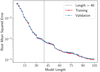 |
Fig. 1. Pareto front of solutions found by OPERON for |

We observe that the error on the prediction decreases rapidly as one initially increases the model length, but this improvement becomes slower after a model length of approximately 30, where the root mean squared error is already at 0.1%. Given that we do not expect to require models that are much more accurate than this, to balance accuracy and simplicity, we choose to select a model from this region, although we note that more accurate models are achievable if one further increased the model length.
As such, after inspecting these equations, we chose the model with length 40 as our fiducial result. This is given by
 (5)
(5)
with the parameters c given in Table 2. This expression achieves a root mean squared error on 0.1% on both the training and test sets. We give the most accurate expression we find in Appendix A, which has a root mean squared error of 0.02% on the validation set. We choose not to make this our fiducial model due since it is a long expression, although we encourage the user to use whichever model is preferable given their target accuracy.
To further investigate the performance of this emulator, in Fig. 2 we plot the predicted σ8 for each point on the training and validation LH as a function of the true value, and we also give the fractional error. We see that the fractional error on σ8 is approximately constant as the true values are varied, although for very small values of σ8 the error slightly increases to a maximum deviation of 1% at σ8≈0.5. These small values are incompatible with current observations (Planck Collaboration VI 2020), and thus this small increase in error is unimportant for actual applications of this result.
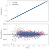 |
Fig. 2. Predicted values (upper) and fractional errors (lower) for the σ8 emulator (Eq. (5)) across the training and validation sets. The root mean squared error is 0.1%, with a maximum error of 1% for very small σ8 values. |
Although we have produced this emulator for an extended cosmology, it is interesting to verify the performance on this emulator in the ΛCDM subspace to ensure that it can be applied to this situation. To do this, we generate a new LH of 2000 cosmologies within the ΛCDM portion of Table 1 and compute the corresponding σ8 values with CLASS. These are then compared against the predictions of Eq. (5) in Fig. 3, where we also show the results of using the emulator proposed in Bartlett et al. (2024a).
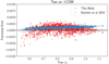 |
Fig. 3. Fractional error on the σ8 prediction for a test set that is restricted to ΛCDM models only. We compare the results of the emulator given here to that of Bartlett et al. (2024a). Our emulator has slightly weaker performance given its extended validity, but the error is almost always within 0.5%. |
As one may expect, given that the emulator of Bartlett et al. (2024a) is specifically optimized for ΛCDM, whereas our method applies to a wider range of cosmologies, we obtain slightly larger emulation errors. We obtain almost identical root mean squared errors of approximately 0.1%, but the distribution of errors has slightly larger tails for this work compared to Bartlett et al. (2024a); our predictions remain almost always within 0.5%, whereas the Bartlett et al. (2024a) emulator has a maximum error of approximately 0.25%. We observe that Bartlett et al. (2024a) systematically overestimates the results. This is due to our use of CLASS instead of CAMB as the ground truth in this paper and since we included neutrino species in CLASS even when mν = 0, which introduces slight deviations from the ΛCDM calculations used in Bartlett et al. (2024a) to obtain their result.
Another observation from Eq. (5) is that most terms are polynomials, except for the log terms. This raises the question of how our SR-derived expression compares to a purely polynomial fit. To investigate this, we performed an experiment where we fit σ8 using polynomials of varying maximum orders and compared the results to our SR emulator. As shown in Fig. 4, a fourth-order polynomial achieves similar accuracy to our SR expression. However, the polynomial fit requires significantly more parameters (330 compared to 16 in Eq. (5)), demonstrating that the SR algorithm can find much more efficient representations compared to standard polynomial fitting.
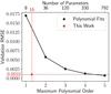 |
Fig. 4. RMSE in the prediction of σ8 for the SR emulator (red point) compared to polynomial fits of varying maximum order (black line). |
5. Analytic emulator for the linear power spectrum
We now consider the task of obtaining a symbolic approximation for the linear matter power spectrum. In the spirit of Bartlett et al. (2024a), rather than attempt to learn  in its entirety, we use some pre-existing approximations for the linear matter power spectrum, so that we only have to learn small corrections to these physics-informed formulae.
To incorporate previous approximations, we find that it is useful to write the linear matter power spectrum as
 (6)
(6)
where θ contains all cosmological parameters, whereas θΛCDM={As, Ωm, Ωb, h, ns} are the subset of parameters describing ΛCDM. We utilized existing results for two of these terms: Dapprox (an approximation for the growth factor) and PΛCDM (an approximation for the ΛCDM linear power spectrum). We note that PΛCDM gives the shape of the linear matter power spectrum, which is equal to redshift-zero power spectrum up to some normalization, which the other terms provide.
We therefore have to learn two terms that give corrections to this:
-
 : This corresponds to (the square of) the correction to the linear growth factor approximation, Dapprox.
 -
 : This is the correction to the redshift-zero linear power spectrum when moving from ΛCDM to the more general cosmological models.
These terms are defined such that  . Although one could make R depend on k, we found that the symbolic expressions we obtained when allowing for this dependence did not include k, and therefore we do not include this argument of the function.
We choose to fit for these corrections to ΛCDM rather than repeat the full fitting procedure of Bartlett et al. (2024a) given that we expect the shape of the BAOs to be independent of the neutrino mass and dark energy equation of state. Given that we already have a precise approximation of these in ΛCDM, it is simpler to fit the broadband corrections to the shape of the power spectrum, which should vary slowly in k and relatively smoothly in time.
In this section, we begin by describing the approximations we use from the literature to give Dapprox (Sect. 5.1) and PΛCDM (Sect. 5.2). We then fit the correction terms to this in Sect. 5.3.
5.1. Approximation for the growth factor
To obtain the time-evolution of the linear matter power spectrum, we wish to have an approximation that we can correct with SR. Fortunately such an approximation already exists. We begin by defining the equality redshift as
 (7)
(7)
Then, defining the time-dependent dark energy and dark matter density parameters as
 (8)
(8)
 (9)
(9)
we use the following approximation for the growth factor in the absence of neutrinos (Lahav et al. 1991; Carroll et al. 1992; Eisenstein & Hu 1998)
 (10)
(10)
If mν≠0, then we must correct this to describe the suppression by neutrinos. We always assume that we have Nν = 3 neutrinos when the neutrino mass is nonzero. One can then define the density parameters of neutrinos and cold dark matter as (Kolb & Turner 1990)
 (11)
(11)
and then the fractional parameters for each species as
 (12)
(12)
We then utilized the approximations for the effects of neutrinos on the growth factor of Bond et al. (1980), Hu & Eisenstein (1998), which are
 (13)
(13)
 (14)
(14)
 (15)
(15)
 (16)
(16)
An approximation of the growth factor can then be written as
 (17)
(17)
where we choose a normalization such that Dapprox→a as a→0.
5.2. ΛCDM power spectrum
To give an approximate template for the matter power spectrum at redshift zero, we used the results of Eisenstein & Hu (1998), Bartlett et al. (2024a). To do this, we define ωm≡Ωmh2 and ωb≡Ωbh2, and define the following variables
 (18)
(18)
 (19)
(19)
 (20)
(20)
 (21)
(21)
 (22)
(22)
 (23)
(23)
 (24)
(24)
where k is measured in h Mpc−1 and TCMB is the temperature of the CMB (which we assume to be 2.7255 K throughout (Mather et al. 1999)). Given this, one can write the Eisenstein & Hu (1998) “no-wiggles” power spectrum at z = 0 as
 (25)
(25)
where kpivot = 0.05 hMpc−1. This describes the overall envelope of the matter power spectrum correctly, but does not contain BAOs.
To approximate the redshift-zero power spectrum in ΛCDM, we define
 (26)
(26)
where we use the approximation of Bartlett et al. (2024a) to evaluate F(k, θ):
![Mathematical equation: $$ \begin{aligned} & \log F = b_0 h - b_{1} + \left (\frac {b_2 \Omega _{\mathrm {b}}}{\sqrt {h^2 + b_3}} \right )^{b_4 \Omega _{\mathrm {m}}} \\ & \times \Biggl [ \frac {b_5 k - \Omega _{\mathrm {b}}}{\sqrt {b_6 + (\Omega _{\mathrm {b}} - b_7 k)^2}} b_8 (b_9 k)^{-b_{10} k} \cos \left (b_{11} \Omega _{\mathrm {m}} - \frac {b_{12} k}{\sqrt {b_{13} + \Omega _{\mathrm {b}}^2}} \right ) \\ & - b_{14} \left (\frac {b_{15} k}{\sqrt {1 + b_{16} k^2}} - \Omega _{\mathrm {m}} \right ) \cos \left (\frac {b_{17} h}{\sqrt {1 + b_{18} k^2}} \right ) \Biggl ] \\ & + b_{19} (b_{20} \Omega _{\mathrm {m}} + b_{21} h - \log (b_{22} k) + (b_{23} k)^{- b_{24} k}) \cos \left (\frac {b_{25}}{\sqrt {1 + b_{26} k^2}} \right ) \\ & + (b_{27} k)^{-b_{28} k} \left (b_{29} k - \frac {b_{30} \log (b_{31} k)}{\sqrt {b_{32} + (\Omega _{\mathrm {m}} - b_{33} h)^2}} \right ) \\ & \times \cos \left (b_{34} \Omega _{\mathrm {m}} - \frac {b_{35} k}{\sqrt {b_{36} + \Omega _{\mathrm {b}}^2}} \right ), \end{aligned} $$](/articles/aa/full_html/2025/06/aa52854-24/aa52854-24-eq44.gif) (27)
(27)
where the parameters b are given in Table 2 of Bartlett et al. (2024a). This approximation gives a linear power spectrum that has a root mean squared fractional error of 0.2% across the k values and ΛCDM portion of the parameter range considered in this work (Bartlett et al. 2024a) when multiplied by the appropriate linear growth factor.
5.3. SR corrections to the linear power spectrum
The approximations outlined in Sects. 5.1 and5.2 yield reasonable approximations of the matter power spectrum, but do not have sub-percent precision. Even when restricted to the ΛCDM subspace, since Dapprox is only an approximation, we find that errors on Plin(k) can still be up to a few percent. Therefore, in this section we use SR to correct for these errors.
5.3.1. Corrections to the growth factor
To obtain a correction to the growth factor, R(a, θ), we generate two LHs of 2000 cosmologies from Table 1, one for training and one for validation. We used 200 logarithmically spaced k values in the range 9×10⁻³−9 h Mpc−1 and compute R, as defined in Eq. (6), and using the results of Sects. 5.1 and 5.2. We find the mean over these k values, and this is then fit as a function of cosmological parameters and scale factor using OPERON, where we search for expressions containing the operators +, −, ×, ÷,  and log. The pow operator is excluded as we found it tends to produce nested power terms, which are both unphysical and numerically unstable. We allow a maximum model length of 100 and set ϵ = 10−3.
After running for 1 hour on 56 cores, we obtain the Pareto front plotted in Fig. 5. As with our σ8 emulator, we find very similar training and validation losses for all model lengths. The improvement in accuracy as one makes the model more complex slightly plateaus at a length of ∼50, at which point the root mean squared error is below 0.1%. We therefore choose a model for R from this region of the Pareto front, and, after inspection, choose the model of length 53.
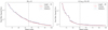 |
Fig. 5. Pareto front of solutions for the correction to the growth factor, R(a, θ), (left), and the correction to the redshift-zero matter power spectrum, 10log10S(k, θ), (right) as found by OPERON. The chosen models are indicated by the vertical lines, and we plot the root mean squared errors on the predictions for the training and validation sets separately. |
Although we defined R(a = 1, θ) = 1 ∀θ, the SR result does not return this exactly due to the finite precision of the parameters and the fact that this is only inferred from the training data, rather than strictly enforced during the search. As such, we find that some parameters that are approximately equal must be equated and that some parameters must be rounded in order to require this condition exactly. After performing such manipulations, we arrive at the following approximation for R(a, θ)
![Mathematical equation: $$ \begin{aligned} R & \left (a, {\boldsymbol {\theta }} \right ) \approx 1 + (1-a) \biggl [d_0 \\ & - \frac {1}{d_1 a + d_2 + \left (d_3 \Omega _{\mathrm {m}} + d_4 a \right ) \log {\left (d_5 w_0 + d_6 w_a \right )}} \\ &- \frac {d_7 \Omega _{\mathrm {m}} + d_8 a + \log {\left (d_9 w_0 + d_{10} w_a \right )}}{d_{11} a + d_{12} + d_{13}\left (d_{14} \Omega _{\mathrm {m}} + d_{15} a - 1\right ) \left (d_{16} w_0 + d_{17} w_a + 1\right )} \biggr ], \end{aligned} $$](/articles/aa/full_html/2025/06/aa52854-24/aa52854-24-eq46.gif) (28)
(28)
where the parameters d are given in Table 3. It is trivial to see that this equals unity at a = 1 for any set of cosmological parameters.
This expression is interesting since, although we allowed OPERON to obtain a function of any combination of cosmological parameters, we find that only Ωm, w0 and wa appear in Eq. (28). Given that these are the parameters that govern the expansion history (alongside h), this suggests that this equation is correcting for the mistakes made in modeling the background expansion when using Dapprox. Although mν do not appear in this equation, it does not mean that there is is no time-dependence in the effects of neutrino suppression on Plin(k, a, θ), but just that Dapprox captures this effect sufficiently well for sub-percent level predictions.
5.3.2. Corrections to the present-day linear power spectrum
The next step is to obtain a correction, S(k, θ), to the redshift-zero power spectrum. This correction depends on k, therefore the training set size is expanded by the number of k values, making it challenging to use a large training size. During our experiments, we found that having a shorter evaluation time was more crucial for achieving good results than using a large number of training examples. Training with 2000 samples in this case was not only computationally expensive but also led to worse convergence. We found that LHs of 200 cosmologies with 200 logarithmically spaced k values in the range 9×10⁻³−9 h Mpc−1 is sufficient for training an accurate S(k, θ). We then compute S, as defined in Eq. (6), and using the results of Sects. 5.1 and 5.2. We choose our target variable to be 10log10S(k, θ) so that (i) the emulated S(k, θ) will always be positive, (ii) a root mean squared error on the target corresponds to minimizing the fractional error on S(k, θ), and (iii) we introduce the factor of 10 to make the target closer to unity. This is then fit as a function of cosmological parameters and k values using OPERON, where we search for expressions containing the operators +, −, ×,  , log, cos, pow and analytic quotient operators (
 ). We add cos as we expected it to make corrections to oscillatory behavior, and we replace ÷ with the analytic quotient operator because the former tends to use k and mν as denominators, which can be zero. We allow a maximum model length of 100 and set ϵ = 10−3.
After running for 6 hour on 56 cores, we obtain the Pareto front plotted in Fig. 5. We see that the Pareto front is considerably flatter for large model lengths than the previous cases, namely that there is little improvement in accuracy when one makes the model more complex. We therefore choose an expression from the start of the flat region of the Pareto front, and find that the expression at length 46 is appropriate for our purposes.
As well as merging and removing superfluous parameters, we find that it is necessary to remove one term from this equation. The expression found by OPERON contained a term that, when we evaluate the model for a ΛCDM universe, was proportional to k. Given that the expression from Bartlett et al. (2024a) is a good approximation for ΛCDM universes, one would expect that S(k, θ) would be independent of k for these cosmologies, and would simply scale the growth factor to correct for the mistakes obtained when using an approximate version, since the shape of Plin(k, a, θ) should be correct. Since the coefficient for this k-dependent term was small ( ), we set this coefficient to zero to remove this term. After removing this term, we re-optimized the coefficients of the function using the training set. We find that the omission of this term has a negligible effect on the accuracy of the expression.
After performing these manipulations, we arrive at the expression
 (29)
(29)
when the coefficients, e, are tabulated in Table 4. We note that the ÷ operation in the fourth term is simplified from the analytic quotient operator.
There are several interesting features in this approximation. Firstly, let us consider the ΛCDM limit, where we have w0=−1, wa = 0 and mν = 0
 (30)
(30)
which is not zero, and thus we have a correction even for these cosmologies. Given that R(a, θ) is unity at redshift zero so cannot correct for errors in Dapprox, this term gives a correction to the growth factor at a = 1 due to using an approximation of this. This term provides a correction to the result of Bartlett et al. (2024a), as given in Eq. (27). This k-independent correction adjusts the normalization of the redshift-zero linear power spectrum, which arises since Bartlett et al. (2024a) fit the residuals between CAMB and the Eisenstein & Hu (1998) prediction, as returned by the COLOSSUS package. In COLOSSUS, the normalization is set such that the result of computing Eq. (2) with the approximate power spectrum matches the desired σ8. Given the limitations of the Eisenstein & Hu (1998) approximation, this induces a multiplicative scaling to the power spectrum that can given errors of a few percent on large-scales (i.e., if one inferred As from the low-k behavior of the COLOSSUS power spectrum, one would find a value that is wrong by a few percent). Although Eq. (27) removes this offset, since in this work we do not attempt to match σ8 in this way, Eq. (30) acts to reintroduce this offset so that Eq. (27) yields the correct result.
Let us also consider the limiting behavior of Eq. (29). On large-scales (k→0), one observes that S(k, θ) tends to a constant, and thus introduces a multiplicative correction due to imperfections induced by the other approximations. It is essential that there is no k-dependence in this limit, since the power spectrum must be proportional to kns on large-scales, and this is already captured by Eq. (25). We also note that on small scales (k→∞), S(k, θ) also tends to a (different) constant. This implies that the other terms in the approximation yield the correct k-dependence on small scales. We note that it is desirable that this term does not diverge even when extrapolated to large k, which is neither guaranteed nor analytically testable for a numerical emulator.
Finally, we note that, although we allowed such behavior, Eq. (29) does not contain any oscillatory terms. This is understandable since one would not expect the interaction between photons and baryons that give rise to the BAO features to depend on the nature of dark energy nor the sum of neutrino masses: these additional components should only affect the broadband features of the power spectrum. This is indeed what we find, and further justifies our decision to find a correction to the ΛCDM result from Bartlett et al. (2024a) rather than refit the whole equation, given the (hard to fit) oscillatory features are unchanged.
5.3.3. Performance of combined approximation
Now that we have verified that the individual components of the linear matter power spectrum are accurately approximated, we combine these approximations of assess the performance of Plin(k, a, θ) across the cosmologies and redshifts considered in this work. Using a LH of 2000 points from the prior range in Table 1, we compare the predictions from the expressions obtained in this work to the true linear power spectrum, as computed using CLASS. We consider both the full parameter space and a separate LH where we restrict ourselves to ΛCDM only. The resulting distribution of errors as a function of k are plotted in Fig. 6, where the bands correspond to the 68th and 95th percentiles of errors across the test set at a given k. Again, we consider 200 values of k that are logarithmically spaced between 9×10⁻³ and 9 h Mpc−1.
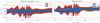 |
Fig. 6. Distribution of fractional errors on Plin(k, a, θ) as a function of k for the extended cosmological models considered in this work (left) and for ΛCDM (right). The bands given the 1 and 2σ values across the LH (Table 1), with the dashed lines indicating 1% error. When averaged over k, we find that our expressions have a root mean squared error of 0.28% for the extended cosmology, and 0.41% for ΛCDM. |
We find that the root mean squared error at any given value of k is much less than 1%, and is 0.28% for the full parameter space when averaged over k and redshift. This increases to 0.41% when we consider the ΛCDM sub-space, which is approximately a factor of 2 less accurate than the approximation of Bartlett et al. (2024a). We attribute this the fact that zero neutrino mass is towards the edge of the range of our training set, where one would expect less accurate results. We explore this point further in Sect. 7.2. Nonetheless, we find that the 2σ error band when varied as a function of k is almost always within 1%. We assess the performance of this approximation further in Sect. 7.1, where we compare to other emulators and fitting functions.
6. Analytic emulator for the nonlinear power spectrum
Now that we have symbolic emulators for quantities related to the linear power spectrum, in this section we aim to produce an approximation for the nonlinear case. To obtain such an expression, one must have access to Pnl(k, a, θ) for a range of cosmological parameters and redshifts. As in Bartlett et al. (2024b), we obtained these by evaluating EUCLIDEMULATOR2 (Euclid Collaboration: Knabenhans et al. 2021), a method known for its speed and accuracy in predicting the ratio of the nonlinear to linear matter power spectrum. This approach was preferred over generating new N-body simulations, as it is significantly less computationally demanding. EUCLIDEMULATOR2 provides percent-level accuracy, allowing us to fit the emulated spectra with high precision and offering greater flexibility in selecting redshift values. Our results are validated against N-body simulations, as discussed in Sect. 7.1.
Unlike Bartlett et al. (2024b), where corrections are applied to an existing HALOFIT formalism, our approach directly fits the nonlinear power spectrum, Pnl, as a function of k, a, θ, and Plin(k, a, θ). By doing this, we avoid fitting additional HALOFIT variables, which can introduce further uncertainties. This method provides a more straightforward and potentially more accurate model for predicting the nonlinear power spectrum, since we do not have to correct for mistakes made by using a previous approximation.
Similar to S(k, θ), we used a LH sampling of 200 cosmologies with 200 logarithmically spaced k values in the range 9×10⁻³−9 h Mpc−1 to generate the training set. For each cosmology, we generated the corresponding nonlinear power spectrum using EUCLIDEMULATOR2. Since the nonlinear emulator requires Plin as input, during training we used ground truth values computed by CLASS. However, for evaluating performance, we employed the Plin emulator developed in Sect. 5.
We fit the nonlinear power spectrum Pnl(k, a, θ, Plin) using OPERON. The model searches for expressions composed of the operators +, −, ×, ÷,  , log, and pow . We found that excluding the analytic quotient operator improves the limiting behavior, as it is easier to enforce the correct limits (discussed below) to the found expressions when this operator was removed. We set our target to log10Pnl and transform the input Plin to log10Plin as well. We allow a maximum model length of 200, and we use the root mean squared error as the loss function, with ϵ = 10−3. After running for 24 hours on 56 cores, we obtain the Pareto front shown in Fig. 7. From this, we select the expression with a model length of 73. The resulting equation (31) is presented below.
 (31)
(31)
where the best-fit parameters are given in Table 5. We denote this expression  rather than Pnl, since it is not our final approximation for the nonlinear power spectrum (see Eq. (33) below).
We find that this equation has several interesting properties. Firstly, one can analytically check the limiting behavior as k→0. In this case, we find that Pnl→Plin as k→0, consistent with our theoretical interpretation. It would not be possible to guarantee such behavior using purely numerical emulators. Second, we observe that mν does not appear explicitly; its dependence is only implicit through Plin. This aligns with the results of Bayer et al. (2022), who found that all the information on the neutrino mass in the large-scale structure is encoded in the linear power spectrum, and not the nonlinear evolution.
When evaluated on both the training and validation set, we observed that this equation by itself introduces a systematic offset compared to the EUCLIDEMULATOR2 results across all cosmologies and redshifts. This is a result of a sub-optimal search of the genetic algorithm, since it was unable to correct for this residual. Therefore, we introduced a post-processing step to correct for this, where we fit and subtracted the offset from the prediction. Again using OPERON with the same settings as before, we fit for the offset as a function of k only. We find that the equation
 (32)
(32)
where h = [0.5787, 2.3485, 27.3829, 16.4236, 97.3766, 90.9764, 11.2046, 2447.2, 11376.93], is sufficient to capture the remaining residual. The final equation for nonlinear power spectrum is then given by
 (33)
(33)
It should be noted that this offset does not affect the limiting behavior as k→0, since the offset tends to zero as k→0. For large k, we find that this offset term does not exactly tend to zero, but oscillates around h1/h8≈2×10−4 with a period Δk = 2π/h4≈0.06 h Mpc−1. Such oscillations give a maximum correction to  of 0.05%, which is much smaller than the error on the power spectrum, and the variation with k is much finer than the values of k for which we reach this limit, which effectively averages out these oscillations. As such, we find that this offset becomes negligible as k→∞.
Using a LH of 2000 points from the prior range in Table 1, we compare our expressions’ predictions to the outputs from EUCLIDEMULATOR2, considering both the full parameter space and a restricted ΛCDM model. The results are given in Fig. 8. The root mean squared fractional error for the two cases is 1.3% and 1.1%, respectively. We find that, in both cases, the error is dominated by the prediction at large k, where the 1σ difference between our result and EUCLIDEMULATOR2 can exceed 1%, whereas the two emulators agree within 1% before k∼1 h Mpc−1. Due to the inclusion of Eq. (32), when compared to Figure 5 of Bartlett et al. (2024b), we find that the residuals of our emulator at the BAOs are smaller and that the mean difference is much closer to zero.
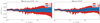 |
Fig. 8. Same as Fig. 6 but for Pnl(k, a, θ, Plin), where we plot the errors relative to EUCLIDEMULATOR2. When averaged over k, we find that our expressions have a root mean squared error of 1.3% for the extended cosmology, and 1.1% for ΛCDM. |
To assess whether this level of disagreement is acceptable, we compare the difference between our symbolic emulator and EUCLIDEMULATOR2 to that between the numerical emulators BACCO and EUCLIDEMULATOR2 over the LH used in this work. In Fig. 9 we plot the 1σ errors across the hypercube for both methods, where we see both our result and BACCO agree within 1% as we go to k→0, as should be expected given than both methods produce sub-percent accurate linear power spectra. Around the scale of the BAOs, the level of disagreement with EUCLIDEMULATOR2 slightly increases to approximately 1% for both emulators. As we increase k further to k>1 h Mpc−1, we find that our error is relatively stable at around 1%, whereas the discrepancy between EUCLIDEMULATOR2 and BACCO rises dramatically to around 4% by k∼4 h Mpc−1. As such, we conclude that the level of disagreement between our approximation and EUCLIDEMULATOR2 is comparable to that between current numerical emulators, and thus we have reached a sufficiently accurate solution. We investigate what this level of disagreement corresponds to for weak lensing measurements in Sect. 7.3.
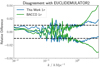 |
Fig. 9. Distribution of fractional differences between different emulators. As a reference we use EUCLIDEMULATOR2, and show the differences between this and the symbolic approximation obtained in this work and the BACCO emulator. We plot the 1σ differences across the LH used in this work, and the dashed lines correspond to 1% agreement. The difference between our result and EUCLIDEMULATOR2 is comparable to the differences between the numerical emulators. |
7. Performance of emulators
7.1. Comparison against other emulators
In this section we assess the performance of our emulator against those from the literature in terms of both run time and accuracy. To assess accuracy, for Plin(k, a, θ), we compare the predicted power spectra to that computed by CLASS. For the nonlinear case, however, it is less obvious what the standard against which we should compare is. In Sect. 6, we calibrated our emulator against EUCLIDEMULATOR2 since this provided a computationally cheap way of generating a large number of spectra at a range of redshifts. Now, however, we wish to compare against a N-body simulation; otherwise, by construction, EUCLIDEMULATOR2 would have zero error. Therefore, as in Bartlett et al. (2024b), we benchmark the nonlinear emulators against the QUIJOTE suite of simulations (Villaescusa-Navarro et al. 2020).
In particular, we test the accuracy against the following four sets simulations
-
Fiducial: This simulation has a ΛCDM cosmology with the Planck 2018 cosmological parameters (Planck Collaboration VI 2020): Ωm = 0.3175, Ωb = 0.049, h = 0.6711, ns = 0.9624, σ8 = 0.834, mν = 0, w0=−1, wa = 0.
-
 : This simulation has a cosmological constant for dark energy, but contains three degenerate massive neutrino species of total mass mν = 0.1 eV. All other parameters are the same as for the Fiducial simulation.
 -
w+: In this simulation the dark energy equation of state is constant in time, but equal to -1.05 (w0=−1.05, wa = 0). All other parameters are the same as for the Fiducial simulation.
-
w−: This is the same as the w+ simulation, except w0=−0.95.
All simulations contain N3 = 5123 particles within a cubic box of side length L = 1 h−1Gpc, and were run using the GADGET-III code (Springel 2005). The simulations containing neutrinos contain an additional 5123 neutrino particles. We make use of the publicly available power spectra for these simulations for k∈[0.02, 0.5] h Mpc−1, since we expect these to be converged in this range (Bartlett et al. 2024b). To remove the effects of cosmic variance (i.e., to obtain an estimate of the ensemble mean power spectra), we average these spectra across all available simulations in each suite (15 000 for the Fiducial simulation and 5000 for the others).
We first compare various linear power spectrum emulators across the four cosmologies. The emulators considered are BACCO (Angulo et al. 2021; Aricò et al. 2021; Zennaro et al. 2023), COSMOPOWER (Spurio Mancini et al. 2022), and three equation-based models from previous works: Eisenstein & Hu (1998), Bartlett et al. (2024a), and Bayron Orjuela-Quintana et al. (2024). Each emulator is applied only to cosmologies that fall within its defined parameter space. Since COSMOPOWER can only be evaluated at fixed k values, we apply linear interpolation to enable comparisons on arbitrary k. Figure 10 shows the relative error as a function of wavenumber k across different cosmologies at redshift 0.
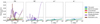 |
Fig. 10. Absolute fractional error on the linear power spectrum as a function of wavenumber, k, for various emulators at redshift 0. We apply each emulator only to test data that falls within its defined parameter space. |
Among the emulators considered, only BACCO and this work can be applied to all four cosmologies, and they show similar errors across the board, which is much less than 1% for all k. For the fiducial cosmology, the numerical emulators (BACCO and COSMOPOWER), the symbolic approximation of Bartlett et al. (2024a), and this work have power spectra that remain within 1% for all k, suggesting these all have the requisite accuracy for modern cosmological analyses. This is not the case for the Eisenstein & Hu (1998) and Bayron Orjuela-Quintana et al. (2024) formulae, whose errors can reach several percent, and are particularly large near the BAOs. Although they have the correct limiting behavior by construction as k→0, their errors are much larger than the subpercent accuracy required for current and future surveys. As highlighted in Taylor et al. (2018), such precision is crucial for unbiased estimation of cosmological parameters from cosmic shear measurements.
To assess the relative runtime of the emulators, we evaluated the linear power spectrum at redshift 1 for the four cosmologies mentioned above, performing 103 evaluations on an Intel Xeon E5-4650 CPU. We report the mean execution time per evaluation. The calculation used 200 logarithmically spaced values of k in the range k = 9×10⁻³−9 h Mpc−1. We assumed the availability of either As or σ8, depending on the emulator's requirements.
The results of this timing test are shown in Fig. 11, where we plot accuracy – computed as the mean absolute fractional error (averaged over k) at redshift 1 across the four cosmologies – against runtime. Our emulator exhibits similar errors (within approximately 0.3%) to BACCO and COSMOPOWER, while being 8 and 80 times faster than them, respectively, on the CPU. Additionally, we include the runtime of two simulators, CLASS and CAMB, showing their differences in simulating the linear power spectrum. We find that our emulator obtains similar errors as there are discrepancies between the two codes (note that by definition CLASS has zero error in Fig. 11), but is a factor 3×10⁴ faster. Although they are of comparable speed to SYREN-HALOFIT and this work, the alternative analytic approximations of Eisenstein & Hu (1998, 1999), Bayron Orjuela-Quintana et al. (2024) are significantly less accurate, with mean errors much greater than a percent, and maximum errors of several percent (see Fig. 10). We find that the result of this work is faster than Bartlett et al. (2024a), which is to be expected given that we have removed the integral associated with using the COLOSSUS package (see Sect. 5.3.2).
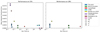 |
Fig. 11. Mean absolute fractional error (averaged over 200 logarithmically spaced k∈[9×10⁻³, 9] h Mpc−1) with respect to CLASS against run time for various linear power spectrum emulators at four cosmologies and redshift 0. Some emulators are tested on both CPU (left panel) and GPU (right panel). The different colors refer to the emulator used, whereas each cosmology (defined in Sect. 7.1) is denoted by a different symbol. |
Two of the emulators (BACCO and COSMOPOWER) are implemented in TensorFlow, making them more efficient for GPU execution. To account for this, we compare a PyTorch implementation of our emulator and of SYREN-HALOFIT with BACCO and COSMOPOWER. We run these four emulators on an NVIDIA Tesla V100 GPU, using a batch size of 2000 for each emulator, and compare their performance. The results are shown in the right panel of Fig. 11, where we see that all emulators are significantly faster. However, due to its simplicity, we still find that our emulator is an order of magnitude faster than both COSMOPOWER and BACCO, with an evaluation time of less than 2 μs. Again, we find SYREN-NEW to be faster than SYREN-HALOFIT.
We also conducted similar comparisons with several nonlinear emulators: EUCLIDEMULATOR2 (Euclid Collaboration: Knabenhans et al. 2021), BACCO (Angulo et al. 2021; Aricò et al. 2021; Zennaro et al. 2023), COSMOPOWER (Spurio Mancini et al. 2022), SYREN-HALOFIT (Bartlett et al. 2024b), and the HALOFIT (Smith et al. 2003; Bird et al. 2012; Takahashi et al. 2012) implementation in CLASS. EUCLIDEMULATOR2 and BACCO are trained to predict the ratio of the power spectrum of N-body simulations to the linear one, whereas COSMOPOWER replicates the results of HMCODE (Mead et al. 2021), which is a semi-analytic approach based on the halo model. These emulators were compared against QUIJOTE simulations across four suites and at three different redshifts (0, 0.5 and 1.5). Since COSMOPOWER has two additional free parameters – cmin, which describes the minimum halo concentration, and η0, which determines the halo bloating – we optimized these parameters to minimize the mean squared error between the prediction of log10Pnl and that from QUIJOTE. The timing results for COSMOPOWER do not include this optimization time and refers to a single pass once cmin and η0 are known.
The results, shown in Fig. 12 as absolute fractional errors, indicate that our emulator performs similarly to EUCLIDEMULATOR2 and BACCO across all suites. SYREN-HALOFIT is applicable only to the fiducial case and shows comparable errors to our method. In contrast, COSMOPOWER and CLASS-HALOFIT generally exhibit larger errors compared to our results. Fig. 13 displays the timing results against the mean absolute fractional error. Our emulator is shown to be 40 times faster than BACCO and 104 times faster than EUCLIDEMULATOR2 on a CPU, all while maintaining comparable error levels. As before, we also compare a PyTorch implementation of our emulator with the two TensorFlow-based emulators in the right panel. We find that our emulator is 65 times faster than COSMOPOWER and 33 times faster than BACCO, and again takes approximately 2 μs to evaluate.
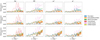 |
Fig. 12. Absolute fractional error on the nonlinear power spectrum as a function of wavenumber, k, for various emulators at redshifts 0, 0.5 and 1. We apply each emulator only to test data that falls within its defined parameter space. |
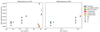 |
Fig. 13. Same as Fig. 11, but now comparing nonlinear emulators with the QUIJOTE simulations and averaging over k∈[0.02, 0.5] h Mpc−1. |
7.2. Error distribution
Our results demonstrate that our linear emulator can achieve a root mean squared fractional error of less than 0.3%, and this is around 1% for the nonlinear emulator on the test set, which is sampled from our wide prior range. However, in applications such as inference problems, accuracy around the true cosmology is often more critical. To illustrate how the error varies with the distance from our current best-fit cosmology, we use cosmological constraints from the Planck + BAO + RSD + SN + DES chains of Alam et al. (2021). Specifically, we fit the marginal posteriors using a multivariate Gaussian distribution and define the distance of a given model from the fiducial one as the probability density provided by the Gaussian. For interpretability, we express this distance in terms of σ values. We generate several new test sets within 1, 3, 5, 7, and 9σ, sampling parameters to be uniformly distributed in this range. Additionally, we compare these results to errors across the entire prior space.
The Alam et al. (2021) study does not provide posteriors that include all three of the w0, wa and mν parameters. Consequently, we cannot directly define a distance metric in our parameter space using their results. Therefore, we consider two subspaces of the eight-dimensional prior space: the ΛCDM parameters (As, Ωm, Ωb, h, ns) combined with w0 and wa, and the ΛCDM parameters combined with mν and w0. These two posteriors define the distance in their respective subspaces, while we fix the remaining parameters as assumed by Alam et al. (2021).
Figure 14 displays the distribution of errors as a function of distance from the best-fit model. For the w0waCDM model, we find that the error decreases as we approach the center of the posterior, such that the error on the linear power spectrum is below 0.2% within 1σ of the posterior mean, and this is below 0.5% for the nonlinear case, which is over a factor of two better than across the full prior range.
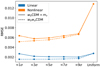 |
Fig. 14. Distribution of errors of the linear (blue) and nonlinear (orange) emulator as a function of distance from the best-fit model in the w0waCDM subspace (dashed lines) and the w0CDM+mν subspace (solid lines). The x axis represents the maximum σ value used for generating the test set. The “Uniform” case corresponds to generating test samples by uniformly sample parameters in the whole prior range. |
In the w0CDM+mν subspace, although the error is smaller near the center compared to the uniformly sampled test set, it increases slightly when approaching the mν = 0 point. This increase is due to the boundary effect in training: the lower limit for mν in the training set is mν = 0, which is problematic since we find empirically that our predictions typically become less accurate near the training set boundaries. For example, we see in Fig. 6 that the massless neutrino model has slight bias when we assume a cosmological constant for dark energy. Nonetheless, in the w0CDM+mν subspace, the error within 9σ of the posterior mean is below 0.3% for the linear power spectrum and still a factor of 2 smaller than for the full prior range when considering the nonlinear emulator.
In the opposite regime, we also wish to understand how our emulators extrapolate outside the range of the training data. Although all emulators (symbolic or numerical) rely on the distribution of training samples, for SR we expect that our results should be able to extrapolate mildly beyond the training prior range. To validate this, we generated several new test sets for our linear emulator and compared the results with those from CLASS. We expanded the nine-dimensional parameter space (eight cosmological parameters plus redshift) by 10% to 30%. For mν and z, we only expanded in the positive direction, while for other parameters, we expanded symmetrically. We found that a 10% extrapolation has a negligible effect on the error, whereas a 20% expansion increases the error to a few percent. However, a 30% extrapolation leads to significant deviations, increasing the error to approximately 10%. We therefore conclude that our emulator indeed extrapolates well outside of the prior range, within a limit of validity that is approximately 20% wider than the range given in Table 1.
7.3. Performance for weak lensing analysis
In Sects. 6 and 7.1, we found that the discrepancy between other emulators or N-body simulations and our approximations is approximately at the percent-level for the nonlinear matter power spectrum, and that this difference is greatest at large k. In this section, we wish to see what this 1% disagreement translates into when we move from just P(k) to precisely analyzing cosmological observations from an upcoming large-scale structure survey and to determine whether this is acceptable or not.
We focus on the upcoming weak lensing observations from the Rubin observatory's Legacy Survey of Space and Time (LSST) (Abell 2009), which directly probes the matter power spectrum. We assess the performance of the model for two stages of the planned observations, year 1 (denoted as LSST Y1) and year 6 (denoted as LSST Y6). Following The LSST Dark Energy Science Collaboration (2018), we assume that LSST Y1 will cover a sky area of fsky = 0.3 and that this will increase to fsky = 0.4 for Y6 analyses.
For these observations, the source samples are expected to follow a distribution given by
![Mathematical equation: $$ n^{\mathrm {tot}}_{\kappa }(z) \propto z^2 \exp [-(z/z_{\mathrm {pz; 0}})^{\alpha _{\mathrm {pz}}}], $$](/articles/aa/full_html/2025/06/aa52854-24/aa52854-24-eq59.gif) (34)
(34)
which is normalized by the effective number density  . For LSST Y1, we assume
  , αpz = 0.87, and zpz;0 = 0.191; for LSST Y6, we assume
  , αpz = 0.798, and zpz;0 = 0.178 (The LSST Dark Energy Science Collaboration 2018). This total distribution is divided into five tomographic bins with equal number densities for each bin i,
  . For shape noise, we expect σe = 0.26/component.
Given these source distributions, we compute the tomographic cosmic shear power spectra as a function of angular scale ℓ as
 (35)
(35)
where, i, j are the indices of tomographic bins, k=(ℓ+1/2)/χ, χ is the comoving distance to redshift z, the integral is performed between zmin = 0 and zmax = 3.0, and  is the lensing efficiency given by:
 (36)
(36)
Here,  represents the normalized redshift distribution of the source galaxies corresponding to the tomographic bin i.
Next, we calculate the covariance for the auto- and cross-correlations of cosmic shear power spectra for the five tomographic bins. In this work, we assume a Gaussian covariance, as was described in Takada & Jain (2004). We ignore the contributions non-Gaussian contributions arising from the tri-spectrum of matter fluctuations (Sato & Nishimichi 2013) and super-sample covariance (Krause & Eifler 2017). The super-sample covariance has been shown to be non-negligible for current and future-generation weak lensing surveys (Barreira et al. 2018). However, we remain conservative in our analysis choices and ignore their contributions here when quantifying the accuracy of our emulator.
To compare the effects of using different matter power spectra, for a LSST-like survey we need to be able to evaluate P(k, z) for approximately k≲10h−1 Mpc−1 and for z<3. Given the coarse spacing of the snapshots of the QUIJOTE simulation, unlike in Sect. 7.1, we choose not to use this as a benchmark as it is not clear that the interpolation required between redshifts would be accurate. Instead, we compare the predictions of different emulators, to see if their differences result in significantly different Cℓ's. Given the large discrepancies between CLASS-HALOFIT and COSMOPOWER when compared against QUIJOTE (Fig. 12), we choose not to use these codes in our comparison, but consider those with approximately percent-level agreement: SYREN-HALOFIT, SYREN-NEW, BACCO and EUCLIDEMULATOR2. In fact, we cannot use BACCO since this is only trained up to z = 1.5, and thus cannot be used for higher-redshift surveys like LSST. For the three remaining codes, we assume the flat ΛCDM cosmology h = 0.6766, Ωm = 0.3111, Ωb = 0.0490, σ8 = 0.8102, ns = 0.9665 (Planck Collaboration VI 2020) with massless neutrinos. To compute Cℓ, we evaluate P(k, z) on a 128×128 two-dimensional grid, uniform in log10k and z, where 5×10⁻³≤k / h−1 Mpc−1≤9 and 0<z<3, which we use to numerically perform the integral Eq. (35).
The resulting Cℓ's are plotted in Fig. 15, where we plot the ratio between the predictions from different emulators and that of EUCLIDEMULATOR2, for ℓ<4×10⁴. For reference, we plot the expected measured errors for Y1 and Y6 in bands. Qualitatively, we see that the differences between the predictions are always within the 1σ band for both Y1 and Y6 for these angular scales, indicating that the percent-level disagreement for P(k) does not lead to significant differences on Cℓ. To estimate the range of angular scales for which the emulators do not yield significantly different results, we compute the total Δχ2 between EUCLIDEMULATOR2 and the symbolic emulators when including all scales up to some maximum ℓ<ℓmax. To ensure that this Δχ2 remains less than unity, for SYREN-NEW one would have to use ℓmax = 2000 for Y1 data and ℓmax = 1000 for Y6, as is indicated by the vertical lines in Fig. 15. We note that a full cosmological inference is required to quantify the impact of these Δχ2 on the parameter biases, which will depend on specific analysis choices and observational systematics, and is outside the scope of this study. 3
 |
Fig. 15. Ratio of shear power spectra, Cℓ (Eq. (35)), computed with SYREN-HALOFIT and SYREN-NEW compared to that computed with EUCLIDEMULATOR2 for LSST. The light gray bands indicate the expected uncertainty for year 1 (Y1), whereas the dark bands are for year 6 (Y6). The numbers in the top left of each panel indicate the redshift bins between which we compute the Cℓ's, such that the diagonal panels are auto-spectra and the off-diagonal ones are cross-spectra. To indicate the importance of baryonic effects, in red we plot the ratio of the HMCODE prediction in the presence of baryons (with log10(TAGN/K) = 8) to the dark-matter-only HMCODE prediction. With vertical lines, we show the scales for which the |

On small scales, the effects of baryonic effects (e.g., astrophysical feedback from active galactic nuclei) and intrinsic alignments on the lensing power spectra are expected to be significant and are poorly understood (e.g., see Krause et al. (2021) and references there-in). 4 To estimate their importance, we use the halo model-based formalism, HMCODE (Mead et al. 2021), developed to capture the impact of baryonic feedback using an effective TAGN parameter that controls the energy output from AGNs. In Fig. 15 we plot the ratio of Cℓ between the HMCODE predictions, when either excluding or including baryonic effects, where we choose an AGN temperature of TAGN = 108 K that is expected from various hydrodynamical simulations (Le Brun et al. 2017; McCarthy et al. 2018). We see that this ratio is much larger than the differences between the dark-matter-only emulators, and thus conclude that the dominant source of uncertainty when used in a weak lensing analysis is not due to the choice of emulator, but due to baryonic effects. As such, we advocate for the use of SYREN-NEW in such an analysis, given its speed and accuracy compared to other emulators (Fig. 13).
8. Conclusion
With current and future surveys poised to probe the massess of neutrinos and the nature of dark energy, rapid and accurate predictions of their effects on the linear and nonlinear evolution of matter in the Universe is essential. In this paper we have used SR to obtain analytic approximations of the linear and nonlinear matter power spectra as a function of redshift and cosmology in the presence of massive neutrinos and dynamical dark energy.
We obtained a succinct correction to previous symbolic approximations of the linear matter power spectrum that is accurate to within 0.3% across a wide range of cosmologies yet is 3×10⁴ times faster than using a Boltzmann code when both are run on a CPU. A further factor of 200 speed-up is possible when running on a GPU. Similarly, we produced a formula to compute the derived parameter σ8 as a function of As and other cosmological parameters, which does not require one to obtain or integrate the linear power spectrum, and is accurate to 0.1%. Analogous to HALOFIT, we found a fitting formula to predict the nonlinear matter power spectrum given the linear one, redshift and cosmological parameters. This approximation matches the predictions of EUCLIDEMULATOR2 (Euclid Collaboration: Knabenhans et al. 2021) to within 1.3% across a broad range of parameter space, redshift and wavenumbers, which is comparable to the level of discrepancy between different numerical emulators. The error is halved when considering cosmologies within the 9σ region of current cosmological constraints (Alam et al. 2021), so we have sub-percent agreement for cosmologies of physical interest. We find that the difference does not lead to significantly different predictions for modern, complex, multi-redshift bin, tomographic weak lensing surveys. We validated these predictions against N-body simulations, finding similar accuracy to numerical emulators while being over an order of magnitude faster, both on a CPU and GPU.
Unlike approaches such as HMCODE, our HALOFIT-like procedure does not include the effects of baryonic feedback, which become important on the smallest scales considered in this work. Future work should therefore be dedicated to obtaining baryonic corrections to our approximations so that one can marginalize over or infer these effects in cosmological analyses. We also note that here, as in Bartlett et al. (2024b), we chose to fit our models to the predictions of numerical emulators, which were themselves trained on N-body simulations since this provided an inexpensive method for producing power spectra. There is no fundamental reason to do this, and indeed one could limit the performance of the symbolic expression if the numerical emulator were not sufficiently accurate. As such, in future work it may be desirable to directly fit the symbolic models to simulations rather than use an intermediary numerical emulator.
Symbolic methods continue to demonstrate an ability to produce fitting formulae that are significantly faster to evaluate than numerical approaches without being less accurate. Such formulae are interpretable, and the correct limiting behavior may readily be enforced. These advantages, coupled with the lack of reliance on particular programming languages or packages, will make symbolic methods valuable for a range of emulation tasks in astrophysics and cosmology.
Data availability
The training and test data for the linear power spectrum were generated using CLASS. The training data for the nonlinear power spectrum were obtained from EUCLIDEMULATOR2, and the test data are available at https://quijote-simulations.readthedocs.io/en/latest/access.html. The specific power spectra and cosmological parameters used in this study will be made available upon reasonable request to the corresponding authors. We provide implementations of our emulators at https://github.com/DeaglanBartlett/symbolic_pofk.
Acknowledgments
We thank Marco Bonici, Lukas Kammerer and Gabriel Kronberger for useful comments and suggestions. CS is supported by the National SKA Program of China (grant No. 2020SKA0110401) and NSFC (grant No. 11821303). DJB and SP are supported by the Simons Collaboration on “Learning the Universe.” BDW acknowleges the DIM-ORIGINES-2023, Infinity Next grant. HD is supported by a Royal Society University Research Fellowship (grant no. 211046). PGF acknowledges STFC and the Beecroft Trust. This work has made use of the Infinity Cluster hosted by Institut d’Astrophysique de Paris; we thank Stephane Rouberol for running this cluster smoothly for us. Some of the computations reported in this paper were performed using resources made available by the Flatiron Institute. The Flatiron Institute is supported by the Simons Foundation.
The authors report an error of 1.5% on the transfer function at k∼0.1 h Mpc−1 for this cosmology. The power spectrum is proportional to the square of this quantity, hence the error on the power spectrum is twice as large as this value.
However, as the residuals between our emulators and EUCLIDEMULATOR2 have a complicated shape, we expect a negligible impact on the S8 parameter that weak lensing mainly constrains (Jain & Seljak 1997) and is sensitive to the scale-independent amplitude of the power spectrum.
Note that the Dark Energy Survey uses a range of scale-cuts corresponding to approximately ℓ≲500 (Doux et al. 2022) to mitigate these effects, which is much stricter than our ℓmax.
References
- AbdusSalam, S., Abel, S., & Romão, M. C. 2025, Phys. Rev. D, 111, 015022 [Google Scholar]
- Ahmed, S. N., Anthony, A. E., Beier, E. W., et al. 2004, Phys. Rev. Lett., 92, 181301 [Google Scholar]
- Akeson, R., Armus, L., Bachelet, E., et al. 2019, arXiv e-prints [arXiv:1902.05569] [Google Scholar]
- Alam, S., Aubert, M., Avila, S., et al. 2021, Phys. Rev., D, 103 [Google Scholar]
- Angulo, R. E., Zennaro, M., Contreras, S., et al. 2021, MNRAS, 507, 5869 [NASA ADS] [CrossRef] [Google Scholar]
- Aricò, G., Angulo, R. E., & Zennaro, M. 2021, arXiv e-prints [arXiv:2104.14568] [Google Scholar]
- Bakx, T., Chisari, N. E., & Vlah, Z. 2024, arXiv e-prints [arXiv:2407.04660] [Google Scholar]
- Bardeen, J. M., Bond, J. R., Kaiser, N., & Szalay, A. S. 1986, ApJ, 304, 15 [Google Scholar]
- Barreira, A., Krause, E., & Schmidt, F. 2018, JCAP, 2018, 015 [Google Scholar]
- Bartlett, D. J., Desmond, H., & Ferreira, P. G. 2023, in GECCO ’23 Companion: Proceedings of the Companion Conference on Genetic and Evolutionary Computation, 2402 [Google Scholar]
- Bartlett, D. J., Kammerer, L., Kronberger, G., et al. 2024a, A&A, 686, A209 [NASA ADS] [CrossRef] [EDP Sciences] [Google Scholar]
- Bartlett, D. J., Wandelt, B. D., Zennaro, M., Ferreira, P. G., & Desmond, H. 2024b, A&A, 686, A150 [NASA ADS] [CrossRef] [EDP Sciences] [Google Scholar]
- Bartlett, D. J., Desmond, H., & Ferreira, P. G. 2024c, IEEE Trans. Evol. Comput., 28, 950 [Google Scholar]
- Bayer, A. E., Banerjee, A., & Seljak, U. 2022, Phys. Rev. D, 105, 123510 [NASA ADS] [CrossRef] [Google Scholar]
- Bayron Orjuela-Quintana, J., Sapone, D., & Nesseris, S. 2024, arXiv e-prints [arXiv:2407.16640] [Google Scholar]
- Becker-Szendy, R., Bratton, C. B., Casper, D., et al. 1992, Phys. Rev. D, 46, 3720 [Google Scholar]
- Bird, S., Viel, M., & Haehnelt, M. G. 2012, MNRAS, 420, 2551 [Google Scholar]
- Blas, D., Lesgourgues, J., & Tram, T. 2011, JCAP, 2011, 034 [Google Scholar]
- Bond, J. R., Efstathiou, G., & Silk, J. 1980, Phys. Rev. Lett., 45, 1980 [NASA ADS] [CrossRef] [Google Scholar]
- Burlacu, B. 2023, in Proceedings of the Companion Conference on Genetic and Evolutionary Computation, GECCO ’23 Companion (New York, NY, USA: Association for Computing Machinery), 2412 [Google Scholar]
- Burlacu, B., Kronberger, G., & Kommenda, M. 2020, in Proceedings of the 2020 Genetic and Evolutionary Computation Conference Companion, GECCO ’20 (New York, NY, USA: Association for Computing Machinery), 1562 [Google Scholar]
- Carroll, S. M., Press, W. H., & Turner, E. L. 1992, ARA&A, 30, 499 [NASA ADS] [CrossRef] [Google Scholar]
- Chevallier, M., & Polarski, D. 2001, Int. J. Mod. Phys. D, 10, 213 [Google Scholar]
- Cooray, A., & Sheth, R. 2002, Phys. Rep., 372, 1 [Google Scholar]
- Cranmer, M., Sanchez Gonzalez, A., Battaglia, P., et al. 2020, Discovering Symbolic Models from Deep Learning with Inductive Biases (Curran Associates, Inc.) [Google Scholar]
- David, E. 1989, Genetic Algorithms in Search, Optimization andMachine Learning, (Addison-Wesley Publishing Company, Inc.) [Google Scholar]
- DESI Collaboration (Aghamousa, A., et al.) 2016, arXiv e-prints [arXiv:1611.00036] [Google Scholar]
- DESI Collaboration (Adame, A. G., et al.) 2024, arXiv e-prints [arXiv:2404.03002] [Google Scholar]
- Doux, C., Jain, B., Zeurcher, D., et al. 2022, MNRAS, 515, 1942 [Google Scholar]
- Eisenstein, D. J., & Hu, W. 1998, ApJ, 496, 605 [Google Scholar]
- Eisenstein, D. J., & Hu, W. 1999, ApJ, 511, 5 [Google Scholar]
- Euclid Collaboration (Knabenhans, M., et al.) 2019, MNRAS, 484, 5509 [Google Scholar]
- Euclid Collaboration (Knabenhans, M., et al.) 2021, MNRAS, 505, 2840 [NASA ADS] [CrossRef] [Google Scholar]
- Fendt, W. A., & Wandelt, B. D. 2007a, arXiv e-prints [arXiv:0712.0194] [Google Scholar]
- Fendt, W. A., & Wandelt, B. D. 2007b, ApJ, 654, 2 [NASA ADS] [CrossRef] [Google Scholar]
- Fukuda, Y., Hayakawa, T., Ichihara, E., et al. 1998a, Phys. Rev. Lett., 81, 1158 [Google Scholar]
- Fukuda, Y., Hayakawa, T., Ichihara, E., et al. 1998b, Phys. Rev. Lett., 81, 1562 [Google Scholar]
- Hahn, O., List, F., & Porqueres, N. 2024, JCAP, 2024, 063 [Google Scholar]
- Haupt, R., & Haupt, S. 2004, Practical Genetic Algorithms, 2nd edn. (Wyley) [Google Scholar]
- Heitmann, K., Higdon, D., White, M., et al. 2009, ApJ, 705, 156 [Google Scholar]
- Heitmann, K., Lawrence, E., Kwan, J., Habib, S., & Higdon, D. 2014, ApJ, 780, 111 [Google Scholar]
- Hu, W., & Eisenstein, D. J. 1998, ApJ, 498, 497 [Google Scholar]
- Jain, B., & Seljak, U. 1997, ApJ, 484, 560 [Google Scholar]
- Kolb, E. W., & Turner, M. S. 1990, The Early Universe, 69 [Google Scholar]
- Kommenda, M., Burlacu, B., Kronberger, G., & Affenzeller, M. 2020, Genet. Program. Evolvable Mach., 21, 471 [Google Scholar]
- Krause, E., & Eifler, T. 2017, MNRAS, 470, 2100 [NASA ADS] [CrossRef] [Google Scholar]
- Krause, E., Fang, X., Pandey, S., et al. 2021, arXiv e-prints [arXiv:2105.13548] [Google Scholar]
- Kronberger, G., Burlacu, B., Kommenda, M., Winkler, S. M., & Affenzeller, M. 2024, Symbolic Regression (Chapman & Hall/CRC Press) [CrossRef] [Google Scholar]
- La Cava, W., Orzechowski, P., Burlacu, B., et al. 2021, arXiv e-prints [arXiv:2107.14351] [Google Scholar]
- Lahav, O., Lilje, P. B., Primack, J. R., & Rees, M. J. 1991, MNRAS, 251, 128 [Google Scholar]
- Laumanns, M., Thiele, L., Deb, K., & Zitzler, E. 2002, Evol. Comput., 10, 263 [CrossRef] [Google Scholar]
- Laureijs, R., Amiaux, J., Arduini, S., et al. 2011, arXiv e-prints [arXiv:1110.3193] [Google Scholar]
- Lawrence, E., Heitmann, K., Kwan, J., et al. 2017, ApJ, 847, 50 [Google Scholar]
- Le Brun, A. M. C., McCarthy, I. G., Schaye, J., & Ponman, T. J. 2017, MNRAS, 466, 4442 [Google Scholar]
- Lesgourgues, J., & Pastor, S. 2006, Phys. Rep., 429, 307 [Google Scholar]
- Levenberg, K. 1944, Q. Appl. Math., 2, 164 [Google Scholar]
- Lewis, A., Challinor, A., & Lasenby, A. 2000, ApJ, 538, 473 [Google Scholar]
- Linder, E. V. 2003, Phys. Rev. Lett., 90, 091301 [Google Scholar]
- LSST Science Collaboration (Abell, P. A., et al.) 2009, arXiv e-prints [arXiv:0912.0201] [Google Scholar]
- Ma, C. -P., & Fry, J. N. 2000, ApJ, 543, 503 [Google Scholar]
- Marquardt, D. W. 1963, J. Soc. Indust. Appl. Math., 11, 431 [CrossRef] [Google Scholar]
- Mather, J. C., Fixsen, D. J., Shafer, R. A., Mosier, C., & Wilkinson, D. T. 1999, ApJ, 512, 511 [Google Scholar]
- McCarthy, I. G., Bird, S., Schaye, J., et al. 2018, MNRAS, 476, 2999 [NASA ADS] [CrossRef] [Google Scholar]
- Mead, A. J., Peacock, J. A., Heymans, C., Joudaki, S., & Heavens, A. F. 2015, MNRAS, 454, 1958 [NASA ADS] [CrossRef] [Google Scholar]
- Mead, A. J., Heymans, C., Lombriser, L., et al. 2016, MNRAS, 459, 1468 [Google Scholar]
- Mead, A. J., Brieden, S., Tröster, T., & Heymans, C. 2021, MNRAS, 502, 1401 [Google Scholar]
- Mootoovaloo, A., Jaffe, A. H., Heavens, A. F., & Leclercq, F. 2022, Astron. Comput., 38, 100508 [NASA ADS] [CrossRef] [Google Scholar]
- Nishimichi, T., Takada, M., Takahashi, R., et al. 2019, ApJ, 884, 29 [NASA ADS] [CrossRef] [Google Scholar]
- Orjuela-Quintana, J. B., Nesseris, S., & Sapone, D. 2024, Phys. Rev. D, 109, 063511 [NASA ADS] [CrossRef] [Google Scholar]
- Planck Collaboration VI. 2020, A&A, 641, A6 [NASA ADS] [CrossRef] [EDP Sciences] [Google Scholar]
- Russeil, E., de Franca, F. O., Malanchev, K., et al. 2024, in Proceedings of the Genetic and Evolutionary Computation Conference, GECCO ’24 (New York, NY, USA: Association for Computing Machinery), 961 [Google Scholar]
- Sato, M., & Nishimichi, T. 2013, Phys. Rev., D, 87, 123538 [Google Scholar]
- Seljak, U. 2000, MNRAS, 318, 203 [Google Scholar]
- Smith, R. E., & Angulo, R. E. 2019, MNRAS, 486, 1448 [NASA ADS] [CrossRef] [Google Scholar]
- Smith, R. E., Peacock, J. A., Jenkins, A., et al. 2003, MNRAS, 341, 1311 [Google Scholar]
- Springel, V. 2005, MNRAS, 364, 1105 [Google Scholar]
- Spurio Mancini, A., Piras, D., Alsing, J., Joachimi, B., & Hobson, M. P. 2022, MNRAS, 511, 1771 [NASA ADS] [CrossRef] [Google Scholar]
- Takada, M., & Jain, B. 2004, MNRAS, 348, 897 [Google Scholar]
- Takahashi, R., Sato, M., Nishimichi, T., Taruya, A., & Oguri, M. 2012, ApJ, 761, 152 [Google Scholar]
- Taylor, P. L., Kitching, T. D., & McEwen, J. D. 2018, Phys. Rev. D, 98, 043532 [Google Scholar]
- The LSST Dark Energy Science Collaboration (Mandelbaum, R., et al.) 2018, arXiv e-prints [arXiv:1809.01669] [Google Scholar]
- Turing, A. M. 1950, Mind, LIX, 433 [CrossRef] [Google Scholar]
- Villaescusa-Navarro, F., Hahn, C., Massara, E., et al. 2020, ApJS, 250, 2 [CrossRef] [Google Scholar]
- Weinberg, D. H., Mortonson, M. J., Eisenstein, D. J., et al. 2013, Phys. Rep., 530, 87 [Google Scholar]
- Winther, H. A., Casas, S., Baldi, M., et al. 2019, Phys. Rev. D, 100, 123540 [CrossRef] [Google Scholar]
- Zennaro, M., Angulo, R. E., Pellejero-Ibáñez, M., et al. 2023, MNRAS, 524, 2407 [Google Scholar]
- Zhai, Z., Tinker, J. L., Becker, M. R., et al. 2019, ApJ, 874, 95 [CrossRef] [Google Scholar]
Appendix A: Most accurate analytic expression found for σ8
Here, we present an analytical approximation for σ8 that, unlike Eq. (5), which attempts to balance accuracy and simplicity, is the most accurate one found. This is the model at length 89 in Fig. 1 and is given by
 (A.1)
(A.1)
where the parameters  are given in Table A.1. Although this form is rather long, we include it in case a more accurate conversion is required. We find that it has a root mean squared error on the w0waCDM+mν and ΛCDM test sets of 0.02% and 0.04%, respectively. We plot the variation in this error with the true σ8 value in Fig. A.1. For the w0waCDM+mν model, the errors are significantly smaller compared to those in Fig. 2, while for ΛCDM, our results show comparable performance to Bartlett et al. (2024a).
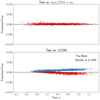 |
Fig. A.1. Fractional error on the σ8 prediction tested on w0waCDM+mν (upper) and ΛCDM (bottom) models using the most accurate σ8 expression (Eq. (A.1)). For the ΛCDM case, we also compare the results of the emulator given here to that of Bartlett et al. (2024a). |
Best-fit parameters for σ8 given in Eq. (A.1).
All Tables
All Figures
|
Fig. 1. Pareto front of solutions found by OPERON for |
| In the text | |
|
Fig. 2. Predicted values (upper) and fractional errors (lower) for the σ8 emulator (Eq. (5)) across the training and validation sets. The root mean squared error is 0.1%, with a maximum error of 1% for very small σ8 values. |
| In the text | |
|
Fig. 3. Fractional error on the σ8 prediction for a test set that is restricted to ΛCDM models only. We compare the results of the emulator given here to that of Bartlett et al. (2024a). Our emulator has slightly weaker performance given its extended validity, but the error is almost always within 0.5%. |
| In the text | |
|
Fig. 4. RMSE in the prediction of σ8 for the SR emulator (red point) compared to polynomial fits of varying maximum order (black line). |
| In the text | |
|
Fig. 5. Pareto front of solutions for the correction to the growth factor, R(a, θ), (left), and the correction to the redshift-zero matter power spectrum, 10log10S(k, θ), (right) as found by OPERON. The chosen models are indicated by the vertical lines, and we plot the root mean squared errors on the predictions for the training and validation sets separately. |
| In the text | |
|
Fig. 6. Distribution of fractional errors on Plin(k, a, θ) as a function of k for the extended cosmological models considered in this work (left) and for ΛCDM (right). The bands given the 1 and 2σ values across the LH (Table 1), with the dashed lines indicating 1% error. When averaged over k, we find that our expressions have a root mean squared error of 0.28% for the extended cosmology, and 0.41% for ΛCDM. |
| In the text | |
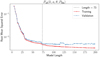 |
Fig. 7. Same as Fig. 5 but for log10Pnl(k, a, θ, Plin). |
| In the text | |
|
Fig. 8. Same as Fig. 6 but for Pnl(k, a, θ, Plin), where we plot the errors relative to EUCLIDEMULATOR2. When averaged over k, we find that our expressions have a root mean squared error of 1.3% for the extended cosmology, and 1.1% for ΛCDM. |
| In the text | |
|
Fig. 9. Distribution of fractional differences between different emulators. As a reference we use EUCLIDEMULATOR2, and show the differences between this and the symbolic approximation obtained in this work and the BACCO emulator. We plot the 1σ differences across the LH used in this work, and the dashed lines correspond to 1% agreement. The difference between our result and EUCLIDEMULATOR2 is comparable to the differences between the numerical emulators. |
| In the text | |
|
Fig. 10. Absolute fractional error on the linear power spectrum as a function of wavenumber, k, for various emulators at redshift 0. We apply each emulator only to test data that falls within its defined parameter space. |
| In the text | |
|
Fig. 11. Mean absolute fractional error (averaged over 200 logarithmically spaced k∈[9×10⁻³, 9] h Mpc−1) with respect to CLASS against run time for various linear power spectrum emulators at four cosmologies and redshift 0. Some emulators are tested on both CPU (left panel) and GPU (right panel). The different colors refer to the emulator used, whereas each cosmology (defined in Sect. 7.1) is denoted by a different symbol. |
| In the text | |
|
Fig. 12. Absolute fractional error on the nonlinear power spectrum as a function of wavenumber, k, for various emulators at redshifts 0, 0.5 and 1. We apply each emulator only to test data that falls within its defined parameter space. |
| In the text | |
|
Fig. 13. Same as Fig. 11, but now comparing nonlinear emulators with the QUIJOTE simulations and averaging over k∈[0.02, 0.5] h Mpc−1. |
| In the text | |
|
Fig. 14. Distribution of errors of the linear (blue) and nonlinear (orange) emulator as a function of distance from the best-fit model in the w0waCDM subspace (dashed lines) and the w0CDM+mν subspace (solid lines). The x axis represents the maximum σ value used for generating the test set. The “Uniform” case corresponds to generating test samples by uniformly sample parameters in the whole prior range. |
| In the text | |
|
Fig. 15. Ratio of shear power spectra, Cℓ (Eq. (35)), computed with SYREN-HALOFIT and SYREN-NEW compared to that computed with EUCLIDEMULATOR2 for LSST. The light gray bands indicate the expected uncertainty for year 1 (Y1), whereas the dark bands are for year 6 (Y6). The numbers in the top left of each panel indicate the redshift bins between which we compute the Cℓ's, such that the diagonal panels are auto-spectra and the off-diagonal ones are cross-spectra. To indicate the importance of baryonic effects, in red we plot the ratio of the HMCODE prediction in the presence of baryons (with log10(TAGN/K) = 8) to the dark-matter-only HMCODE prediction. With vertical lines, we show the scales for which the |
| In the text | |
|
Fig. A.1. Fractional error on the σ8 prediction tested on w0waCDM+mν (upper) and ΛCDM (bottom) models using the most accurate σ8 expression (Eq. (A.1)). For the ΛCDM case, we also compare the results of the emulator given here to that of Bartlett et al. (2024a). |
| In the text | |
Current usage metrics show cumulative count of Article Views (full-text article views including HTML views, PDF and ePub downloads, according to the available data) and Abstracts Views on Vision4Press platform.
Data correspond to usage on the plateform after 2015. The current usage metrics is available 48-96 hours after online publication and is updated daily on week days.
Initial download of the metrics may take a while.