| Issue |
A&A
Volume 686, June 2024
|
|
|---|---|---|
| Article Number | A150 | |
| Number of page(s) | 11 | |
| Section | Cosmology (including clusters of galaxies) | |
| DOI | https://doi.org/10.1051/0004-6361/202449854 | |
| Published online | 05 June 2024 | |
SYREN-HALOFIT: A fast, interpretable, high-precision formula for the ΛCDM nonlinear matter power spectrum
1
CNRS & Sorbonne Université, Institut d’Astrophysique de Paris (IAP), UMR 7095, 98 bis bd Arago, 75014 Paris, France
e-mail: This email address is being protected from spambots. You need JavaScript enabled to view it.
2
Center for Computational Astrophysics, Flatiron Institute, 162 5th Avenue, New York, NY 10010, USA
3
Astrophysics, University of Oxford, Denys, Wilkinson Building, Keble Road, Oxford OX1 3RH, UK
4
Institute of Cosmology & Gravitation, University of Portsmouth, Dennis Sciama Building, Portsmouth PO1 3FX, UK
Received:
5
March
2024
Accepted:
22
March
2024
Abstract
Context. Rapid and accurate evaluation of the nonlinear matter power spectrum, P(k), as a function of cosmological parameters and redshift is of fundamental importance in cosmology. Analytic approximations provide an interpretable solution, yet current approximations are neither fast nor accurate relative to numerical emulators.
Aims. We aim to accelerate symbolic approximations to P(k) by removing the requirement to perform integrals, instead using short symbolic expressions to compute all variables of interest. We also wish to make such expressions more accurate by re-optimising the parameters of these models (using a larger number of cosmologies and focussing on cosmological parameters of more interest for present-day studies) and providing correction terms.
Methods. We use symbolic regression to obtain simple analytic approximations to the nonlinear scale, kσ, the effective spectral index, neff, and the curvature, C, which are required for the HALOFIT model. We then re-optimise the coefficients of HALOFIT to fit a wide range of cosmologies and redshifts. We then again exploit symbolic regression to explore the space of analytic expressions to fit the residuals between P(k) and the optimised predictions of HALOFIT. Our results are designed to match the predictions of EUCLIDEMULATOR2, but we validate our methods against N-body simulations.
Results. We find symbolic expressions for kσ, neff and C which have root mean squared fractional errors of 0.8%, 0.2% and 0.3%, respectively, for redshifts below 3 and a wide range of cosmologies. We provide re-optimised HALOFIT parameters, which reduce the root mean squared fractional error (compared to EUCLIDEMULATOR2) from 3% to below 2% for wavenumbers k = 9 × 10⁻³ − 9 h Mpc−1. We introduce SYREN-HALOFIT (symbolic-regression-enhanced HALOFIT), an extension to HALOFIT containing a short symbolic correction which improves this error to 1%. Our method is 2350 and 3170 times faster than current HALOFIT and HMCODE implementations, respectively, and 2680 and 64 times faster than EUCLIDEMULATOR2 (which requires running CLASS) and the BACCO emulator. We obtain comparable accuracy to EUCLIDEMULATOR2 and the BACCO emulator when tested on N-body simulations.
Conclusions. Our work greatly increases the speed and accuracy of symbolic approximations to P(k), making them significantly faster than their numerical counterparts without loss of accuracy.
Key words: methods: numerical / cosmological parameters / cosmology: theory / large-scale structure of Universe
© The Authors 2024
 Open Access article, published by EDP Sciences, under the terms of the Creative Commons Attribution License (https://creativecommons.org/licenses/by/4.0), which permits unrestricted use, distribution, and reproduction in any medium, provided the original work is properly cited.
This article is published in open access under the Subscribe to Open model. This email address is being protected from spambots. You need JavaScript enabled to view it. to support open access publication.
1. Introduction
Under the current cosmological paradigm, the large-scale structure of the Universe evolved under gravity and cosmic expansion from highly Gaussian density fluctuations in the distant past to the present-day cosmic web. Despite the remarkable simplicity of the standard model (ΛCDM), which contains just six parameters, the nonlinear equations of motion necessitate the computationally non-trivial task of simulating this evolution, which is typically done through expensive N-body simulations. The nonlinear evolution has a dramatic effect on the matter power spectrum, P(k), greatly enhancing the small-scale power compared to linear theory, and thus these effects cannot be neglected. Even linear theory – which is valid on large scales – requires solving a hierarchy of coupled, linear differential equations (Lewis et al. 2000; Blas et al. 2011; Hahn et al. 2023), demonstrating the difficulty in obtaining accurate predictions for P(k).
Given the importance of the power spectrum in cosmological analyses, much effort has been put into by-passing these expensive simulations and directly predicting the matter power spectrum as a function of time and cosmological parameters. Speed and differentiability of surrogate models are particularly attractive features. For example, the first high-precision emulator for the linear outputs of Boltzmann codes, PICO (Fendt & Wandelt 2007a,b) enabled the first use of Hamiltonian Monte Carlo methods for cosmological parameter inference (Hajian 2007) due to these properties.
Approximations to the linear matter power spectrum are well-established, notably those of Eisenstein & Hu (1998, 1999), which are accurate to a few percent, and the earlier work of Bardeen et al. (1986), which provided a less accurate approximation. More recently, simple expressions which obtain a similar accuracy to Eisenstein & Hu were obtained by Orjuela-Quintana et al. (2023, 2024), although these do not have the same physical motivation as the earlier works. However, these symbolic expressions are insufficiently accurate for modern uses. This led Bartlett et al. (2024) to propose a simple extension to the Eisenstein & Hu (1998) expressions which gives a root mean squared fractional error of just 0.2% across a wide range of cosmologies, which is more than sufficient for current analyses (Taylor et al. 2018).
On small scales, however, we must go beyond the linear predictions, and thus fitting formulae for the nonlinear matter power spectrum have proven essential. The scaling ansatz of Hamilton et al. (1991), which assumed that nonlinear structures decouple and form isolated systems, led to the development of the approximation of Peacock & Dodds (1996). More recent approximations generically fall into one of three categories.
The first approach to predicting the nonlinear matter power spectrum is to use emulation techniques such as Neural Networks or Gaussian Processes, which are trained on N-body simulations to directly predict P(k) given a set of cosmological parameters (Heitmann et al. 2009, 2010, 2014; Casarini et al. 2016; Winther et al. 2019; Angulo et al. 2021; Aricò et al. 2021; Euclid Collaboration 2021; Spurio Mancini et al. 2022; Mootoovaloo et al. 2022; Zennaro et al. 2023). The remaining two approaches are based on the halo model (Ma & Fry 2000; Seljak 2000; Cooray & Sheth 2002), which assumes that the matter content of the Universe is bound in dark matter halos. Under the approach adopted by HMCODE (Mead et al. 2015, 2016, 2021), one can predict P(k) by performing integrals of important quantities in the halo model, such as the density profile of halos and the halo mass function, which are assigned simple symbolic expressions. In the HALOFIT model (Smith et al. 2003; Bird et al. 2012; Takahashi et al. 2012), one assumes there are two distinct contributions to the matter power spectrum; on large scales, P(k) is dominated by the two-halo term, which describes correlations between the spatial positions of different halos, whereas on small scales, the one-halo regime, P(k) is governed by the distribution of dark matter within individual halos. These two terms are approximated by analytic functions of the linear matter power spectrum and quantities derived from this (see Sect. 2.1 for more detail).
The advantage of halo-model based approaches is that, involving only analytic expressions, they are much easier to interpret than numerical emulators and have clearer extrapolation behaviour. Moreover, given the limited flexibility of their simple analytic expressions, the emulated predictions typically vary smoothly with input variables, so that the output is less noisy compared to a purely numerical approach (Fendt & Wandelt 2007a). This is particularly desirable when utilising gradient-based optimisation or inference techniques since the derivatives of the analytic expressions will be smoother than their numerical counterparts. Additionally, analytic expressions are highly portable since they can be easily implemented in the user’s preferred programming language and do not become unusable when the codes underlying numerical approaches become deprecated.
However, in their current forms, there are two main disadvantages of the symbolic approaches compared to the emulators. Firstly, both symbolic approaches require one to perform integrals, which can be computationally slow. This is a major problem for current analysis pipelines. Second, they do not have the same level of accuracy as the numerical emulators. The aim of this work is to solve both of these problems, in three steps:
-
We produce simple analytic expressions (Eqs. (25)–(27)) for all variables appearing in the HALOFIT model so that, when coupled with the linear matter power spectrum approximation of Bartlett et al. (2024), HALOFIT can be evaluated without performing any integrals, dramatically increasing its speed by a factor of 2350.
-
We update the parameters of HALOFIT (Eqs. (29)–(38)) to optimise them for cosmologies relevant to present-day applications (see Table 1) This reduces the maximum error from ∼10% for k ≲ 10 h Mpc−1 to ∼5%, when compared against the parameters of Takahashi et al. (2012) across a wide range of cosmologies and redshifts.
-
We provide a simple analytic correction (Eqs. (39) and (40)) which can multiply the standard HALOFIT prediction to produce sub-percent level accurate power spectra. We note that (like all HALOFIT implementations but unlike the numerical emulators) a small residual remains due to imperfect modelling of the baryonic acoustic oscillations, but these are at approximately the percent level. This appears to be an inherent limitation of the HALOFIT formalism and should be addressed in future work.
Range of cosmological parameters and redshift considered when constructing our analytic emulators.
These significant improvements are enabled through the use of symbolic regression (SR) to rapidly and automatically search through the space of candidate fitting functions to yield high accuracy approximations of the various quantities of interest. SR has gained popularity in recent years within the field of physics to re-discover laws of physics from data (Lemos et al. 2023), propose candidate new ones (Bartlett et al. 2023a,b; Desmond et al. 2023; Sousa et al. 2024; Kamerkar et al. 2023; Koksbang 2023b; Lodha et al. 2024; Alestas et al. 2022), provide simple expressions to explain the output of complex simulations (Delgado et al. 2022; Miniati & Gregori 2022; Koksbang 2023a,c; Wadekar et al. 2023), and obtain fitting functions for observed properties of astrophysical systems (Russeil et al. 2022, 2024).
We note that in this paper we focus our attention on ΛCDM models only, whereas emulators such as EUCLIDEMULATOR2 and the BACCO emulator can handle non-zero neutrino mass and an evolving equation of state for dark energy. We leave such extensions to future work.
In Sect. 2 we provide theoretical background by presenting the HALOFIT model and describe the SR method we use to produce analytic approximations. We obtain and present expressions for the variables required for HALOFIT in Sect. 3, and we optimise the parameters of this model in Sect. 4. In Sect. 5 we provide an extension to the traditional HALOFIT model – which we call SYREN-HALOFIT (symbolic-regression-enhanced HALOFIT) – yielding percent level accurate predictions for P(k). Our expressions are validated against an independent set of simulations in Sect. 6, where we also compare to existing emulators in both accuracy and speed. We conclude and discuss future work in Sect. 7. Throughout this paper “log” denotes the natural logarithm, and base-10 logarithms are denoted by “log10”.
2. Theoretical background
2.1. Nonlinear matter power spectrum
We wish to find an analytic approximation to the nonlinear matter power spectrum, P(k; a, θ), for a ΛCDM cosmology as a function of cosmological parameters, θ, scale factor, a = 1/(1 + z), and wavenumber, k. In this paper we focus on the standard ΛCDM model, so θ comprises of the (redshift zero) density parameter for baryons, Ωb, and for all matter, Ωm; the Hubble constant, H0 = 100 h km s−1 Mpc−1; the scalar spectral index, ns; the curvature fluctuation amplitude, As; and the reionisation optical depth, τ. Throughout this paper we use σ8 instead of As, which is defined as
 (1)
(1)
for
 (2)
(2)
where σ8 is evaluated at R = 8 h−1 Mpc. Since τ has a very small effect on the power spectrum, we ignore this parameter throughout. We also set the neutrino mass to zero in all calculations.
In our previous work (Bartlett et al. 2024), we found an analytic emulator for the z = 0 linear matter power spectrum. Given the zero-baryon Eisenstein & Hu fit (Eisenstein & Hu 1998, 1999), PEH(k; θ), we defined
 (3)
(3)
and found an expression for F which was able to produce a sub-percent level approximation to PL(k; a, θ) for a range of cosmologies. Throughout this paper, when referring to this fitting formula, we mean the ‘fiducial’ model given in Bartlett et al. (2024) as opposed to the more accurate yet less interpretable model given in the appendix of that paper.
Extending this to the nonlinear case requires addressing three differences compared to the linear theory prediction:
-
P(k; a, θ) depends on the scale factor, a, in a non-trivial manner.
-
Nonlinear physics smears the baryonic acoustic oscillation (BAO) peaks.
-
Nonlinear physics boosts power on small scales (large k).
To deal with these problems, we first note that it is trivial to scale the z = 0 linear matter power spectrum to a different redshift:
 (4)
(4)
 (5)
(5)
where the linear growth factor is (ignoring radiation)
 (6)
(6)
where 2F1 is the Gauss hypergeometric function.
To address the remaining two problems, we base our approach on HALOFIT (Smith et al. 2003; Takahashi et al. 2012), a commonly used tool to model the nonlinear matter power spectrum. To do this, one defines a few variables based on the linear matter power spectrum. kσ is defined to be the wavenumber at which
 (7)
(7)
for
 (8)
(8)
and PL(k) is the linear matter power spectrum, where for brevity we suppress the dependence on a and θ for the remainder of this section.
Once we have kσ, we also define
 (9)
(9)
 (10)
(10)
Before continuing to describe the details of HALOFIT, it is worth emphasising how computationally demanding this is. First, one must run a Boltzmann solver to obtain the linear matter power spectrum. Then, one must run a root-finding algorithm to solve Eq. (7) for kσ, where each iteration involves performing an integral over k. Once one has identified kσ,  must then be computed for many values of R such that its first and second derivative at kσ can be calculated, either by finite differences or by fitting a spline. This is a large number of steps given that this is meant to be a fast method for approximating P(k).
These variables are then combined to give the prediction for the matter power spectrum. Using the notation of Takahashi et al. (2012), we write
 (11)
(11)
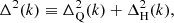
where  is the two-halo term and
  is the one halo term.
Smith et al. (2003) and Takahashi et al. (2012) model the two-halo term as
![Mathematical equation: $$ \begin{aligned} \Delta _{\rm Q}^2(k) = \Delta _{\rm L}^2(k) \left[ \frac{\left( 1 + \Delta _{\rm L}^2(k) \right)^{\beta _n}}{1 + \alpha _n \Delta _{\rm L}^2 (k)} \right] e^{-f({ y})}, \end{aligned} $$](/articles/aa/full_html/2024/06/aa49854-24/aa49854-24-eq15.gif) (12)
(12)
where y ≡ k/kσ, f(y)≡y/4 + y2/8, and the parameters αn and βn are given by (fit from Takahashi et al. 2012)
 (13)
(13)
 (14)
(14)
They then model the one halo term as
 (15)
(15)
![Mathematical equation: $$ \begin{aligned}&{\Delta _{\rm H}^\prime }^2 (k) = \frac{a_n { y}^{3 f_1(\Omega _{\rm m})}}{1 + b_n { y}^{f_2(\Omega _{\rm m})} + \left[ c_n f_3(\Omega _{\rm m}) { y}\right]^{3 - \gamma _n}}. \end{aligned} $$](/articles/aa/full_html/2024/06/aa49854-24/aa49854-24-eq19.gif) (16)
(16)
The parameters an, bn, cn, γn and νn are, noting that w = −1 for our case,
 (17)
(17)
 (18)
(18)
 (19)
(19)
 (20)
(20)
 (21)
(21)
and the functions fi are given by
 (22)
(22)
 (23)
(23)
 (24)
(24)
where Ωm(z) is the total matter density parameter at redshift z.
2.2. Symbolic regression
To provide corrections to HALOFIT, we utilise the supervised machine learning technique of symbolic regression (SR) as implemented in the OPERON package1 (Burlacu et al. 2020). OPERON uses genetic programming (Turing 1950; Goldberg 1989; Affenzeller et al. 2009) to evolve a population of candidate mathematical expressions which attempt to fit a dataset given some inputs. Leveraging operations inspired by natural selection such as mutation and crossover (breeding), over several iterations the population evolves, with new members arising and poorly performing members being discarded. The expectation is that the population evolves to become fitter, and thus more accurate analytic expressions appear as the algorithm progresses. OPERON implements this procedure in a fast and memory efficient manner and has been shown to perform well in benchmark studies (La Cava et al. 2021; Burlacu 2023).
All free parameters in expressions considered by OPERON are optimised (Kommenda et al. 2020) using the Levenberg–Marquardt algorithm (Levenberg 1944; Marquardt 1963). This includes additional scaling parameters, which appear at each terminal node in the expression tree, namely if x is an input variable, then this will always appear as ci × x for a parameter ci, with a different value of ci for each occurrence of x. We define the model length to be the number of nodes appearing in an expression tree, excluding these scaling terms. For example, the function cos(c0 × x) would have a model length of 2 and exp(c0 × x)+c1 × x has a model length of 4.
During non-dominated sorting, the objective values (root mean squared error and model length) of the equations are compared using the concept of ϵ-dominance (Laumanns et al. 2002). There, a hyper-parameter ϵ is supplied to OPERON such that two objective values within a distance ϵ of each other are considered equal, and is chosen to promote convergence of the algorithm. Different values of ϵ are used throughout this paper, which are chosen through experimentation with the aim of obtaining accurate yet compact expressions.
SR is a Pareto-optimisation problem due to the competing objectives of accuracy and simplicity: one can make an equation arbitrarily accurate by making it sufficiently complex, but making it too simple will give inaccurate predictions. However, one would expect that extremely complex models will have a tendency to over-fit the training data, so we use a validation set in all cases to aid this assessment. When selecting models which balance the accuracy-simplicity trade-off, we cannot rely on principled statistical methods developed for SR (see Bartlett et al. 2023a,b) due to the lack of measurement uncertainties in the quantities we wish to approximate. Instead, we begin by only considering those models lying on the Pareto front – the most accurate model of a given length – since these give the set of expressions which maximise one objective given a fixed value of the other. We discard all functions which do not satisfy some predefined accuracy level and those for which the training and validation losses differ significantly. This leaves us with a set of models which we deem yield acceptable fits on both the training and validation datasets. We then choose the “best” model by visually inspecting the remaining expressions and making a subjective judgement based on their functional forms.
3. Analytic approximations to HALOFIT variables
Rather than having to compute each of Eqs. (7), (9), and (10) on the fly (i.e., re-evaluate the linear matter power spectrum for the correct cosmology, perform a root-finding procedure, fit a spline and take derivatives), it would be preferable if each of these variables could be expressed as a simple function of cosmological parameters.
Unlike in Bartlett et al. (2024), we cannot simply compute these quantities at redshift zero and re-scale, since all of kσ, neff and C are dependent on redshift in a non-trivial manner. To generate a training and validation set, we therefore sampled cosmologies from a Latin hypercube using the widths of parameters given in Table 1, but added in an additional parameter, redshift. The range of the parameters are the same as those used to construct EUCLIDEMULATOR2 (Euclid Collaboration 2021) and those used in Bartlett et al. (2024). We sampled redshift uniformly in the range [0, 3], although we symbolically regressed in scale factor a = 1/(1 + z). We generated 200 training and 200 validation points which we fitted to.
We computed kσ, neff and C by performing the integral in Eq. (7) using the linear power spectrum outputted by CAMB (Lewis et al. 2000). We could not use an infinite range of k to perform this integral, but found that using a minimum k, maximum k and logarithmic spacing of k of 10−4 h Mpc−1, 102 h Mpc−1 and 0.003 (corresponding to 2000 k values) gave converged results, where we integrated using Simpson’s rule.
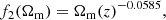
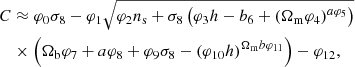
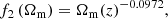
We fitted each of kσ, neff and C as a function of cosmology using OPERON, optimising simultaneously the root mean squared error (MSE) and the length of the model, using the basis operators +, −, ×, ÷,  , pow and log. The Pareto fronts of solutions found are given in Fig. 1, with the settings described in the following sub-sections.
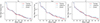 |
Fig. 1. Pareto front of solutions found with OPERON for kσ (left; Eq. (7)), neff (centre; Eq. (9)) and C (right; Eq. (10)) over the range of cosmologies and redshifts considered. We plot the Pareto fronts for the training and validation data separately, indicating the lengths of our preferred models with vertical dotted lines. |
3.1. Analytic approximation of kσ
Since at large redshifts the value of kσ can be large, we find that it is more appropriate to learn log kσ rather than kσ directly. This has the advantage that kσ will always be predicted to be positive. We fitted this variable with OPERON using ϵ = 10−5, running for 4 min or a maximum of 109 function evaluations. From the resulting Pareto front, we see that there is a plateau in goodness of fit between model lengths ∼25–30. Inspecting these equations, we observed that the expression at model length 25 seems reasonable, so we chose this function. OPERON gave an overparameterised form for this function and included an offset term which is much smaller than the error on the fit, so can be neglected. Redefining some parameters and rearranging, we obtain
![Mathematical equation: $$ \begin{aligned}&\log \left( \frac{k_\sigma }{h\,\mathrm{Mpc^{-1}}} \right) \approx \frac{\psi _0}{\sigma _8 \left( a + \psi _9 n_{\rm s} \right)} \left[ \psi _1 a \left( \psi _2 - \sigma _8 \right) \right. \nonumber \\&\quad \left. + \left( \psi _3 a \right)^{-\psi _4 a - \psi _5 n_{\rm s}} \left( \psi _6 \Omega _{\rm b} + \left( \psi _7 \Omega _{\rm m} \right)^{-\psi _8 h} \right) \right], \end{aligned} $$](/articles/aa/full_html/2024/06/aa49854-24/aa49854-24-eq29.gif) (25)
(25)
where ψ = {4.3576, 0.8358, 0.4302, 20.1077, 0.2593, 0.5732, 1.6809, 20.0433, 0.4257, 0.3908}.
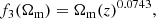
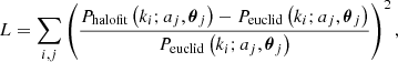
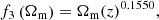
The fractional residuals on the training and validation sets are shown in the left panel of Fig. 2, where we see an approximate percent-level agreement. The root mean squared fractional error on kσ is 0.7% and 0.8% for the training and validation sets, respectively.
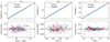 |
Fig. 2. Predicted values (upper) and fractional errors (lower) for kσ (left; Eq. (7)), neff (centre; Eq. (9)) and C (right; Eq. (10)) plotted against their true values, using the results in Eqs. (25)–(27), respectively. The errors are almost always within 2% for kσ, 0.5% for neff and 1% for C. |
3.2. Analytic approximation of neff
Turning our attention to neff, we again set the parameter ϵ = 10−5 and ran for a maximum of 2 min or 108 function evaluations. We see that there is a definitive kink in the Pareto front at a model length of around 17. Given that this is producing a root mean squared error of below 10−2 (in fact it is 0.2% for both the training and validation sets) and it is not overly complicated when visually inspected, we chose this model. We note that Fig. 1 appears to show a significant drop in MSE at a model length of 19, but given the already low error and the appearance of a term containing aa in that expression, we chose the length-17 model. After some simplification, and noting again that the offset term produced by OPERON is much smaller than the error so can be set to zero, this equation is
 (26)
(26)
where χ = {1.6514, 4.8815, 0.5125, 0.1488, 15.6499, 0.2393, 0.1346}. The residuals to this fit are given in the central panel of Fig. 2, from which we see sub-percent fractional errors at all cosmologies and redshifts considered.
3.3. Analytic approximation of C
Moving to a fit for C, we chose ϵ = 10−3 (due to the smaller absolute values of C compared to log kσ and neff) and ran for a slightly longer time than for neff, with a maximum of 4 min or 109 function evaluations. There is a slightly less noticeable kink in the Pareto front (Fig. 1) than for neff, although we see that after a model length of approximately 25, there is a reasonably sharp increase in accuracy, which then flattens up to a model length of approximately 35. Given the low errors in this regime, this seems a sensible place to choose a function from. Inspecting the models of these lengths, we found that many functions contain several nested exponential, which is undesirable. However, the model found with a length of 30 does not have this problem, so we chose this function. This is
 (27)
(27)
where φ = {0.3359, 1.4295, 0.1153, 0.0572, 48.0722, 0.1941, 1.176, 1.0151, 0.2354, 0.3596, 2.3898, 0.3569, 0.4431}.
The fractional residuals of this fit are shown in the right panel of Fig. 2, where we see that we are always accurate within 2%, but almost always within 0.5%. This is reflected in the root mean squared fractional error on C of 0.3% for both the training and validation sets.
4. Optimised HALOFIT parameters
Now we have symbolic expressions for kσ, neff and C, we can rewrite HALOFIT using (1) the Bartlett et al. (2024) linear P(k) emulator and (2) the newly constructed emulators for these variables. Before adding any additional terms, we re-optimised the parameters of HALOFIT using the emulated values of PL, kσ, neff and C. The commonly used parameters of Takahashi et al. (2012) were optimised considering sixteen sets of cosmological parameters: six cosmologies based on the results of WMAP (Spergel et al. 2003, 2007; Komatsu et al. 2009, 2011), and ten taken from the Coyote universe project (Heitmann et al. 2009, 2010; Lawrence et al. 2010). Since then, improved constraints on cosmological parameters mean these may not cover the region of parameter space which is of interest for present-day experiments, with some falling outside the range given by Table 1. Thus, we re-optimised the HALOFIT parameters so that they provide the best possible fits across the range of parameters given in Table 1.
To perform this optimisation, we need access to the nonlinear matter power spectrum. To allow us to use any redshift, we generated P(k; a, θ) using EUCLIDEMULATOR2 (Euclid Collaboration 2021), a fast and accurate method for predicting the ratio of the nonlinear matter power spectrum to the linear one. We chose to do this rather than generate new N-body realisations since such a generation is much more computationally expensive. EUCLIDEMULATOR2 is accurate to the percent level, so we can achieve a high degree of accuracy from fitting the emulated spectra, and this allows more flexibility in choosing redshift values. We validate our results against N-body simulations in Sect. 6.1.
We again used 200 cosmologies drawn from a Latin hypercube with the same bounds as in Sect. 3 (including the addition of redshift). We used 100 logarithmically spaced k values in the range 9 × 10⁻³ − 9 h Mpc−1. Specifically, we optimised the parameters of an, bn, cn, γn, νn, αn and βn and the exponents of f1, f2 and f3. As a loss function, we used the mean fractional squared error on the HALOFIT model compared to EUCLIDEMULATOR2:
 (28)
(28)
where i indexes the 100 values of k and each point on the Latin hypercube is given by scale factor aj and cosmological parameters θj.
We optimised Eq. (28) using an Adam optimiser (Kingma & Ba 2015). The initial learning rate was set to 0.01, and we used the StepLR learning rate scheduler, with a step size of 100 and gamma = 0.9. We ran the optimiser for 2 × 10⁴ iterations, but found that it converged much before this. As an initial guess, we use the parameters used in Takahashi et al. (2012).
After optimising the parameters and rounding to four decimal places, we obtained new expressions for the HALOFIT parameters:
 (29)
(29)
 (30)
(30)
 (31)
(31)
 (32)
(32)
 (33)
(33)
 (34)
(34)
 (35)
(35)
 (36)
(36)
 (37)
(37)
 (38)
(38)
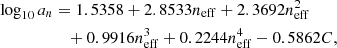
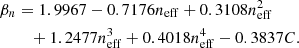
For the remainder of the paper, we refer to the HALOFIT model with these parameters as HALOFIT+. We note that these parameters are not dramatically different to Takahashi et al. (2012), so this represents a small refinement of their fit. We compare the results of this choice of parameters to those of Takahashi et al. (2012) in Fig. 3, where we see a particularly dramatic improvement in the one-to-two halo regime. The root mean squared fractional error for Takahashi et al. (2012) is 2.9% and 3.0% on the training and validation sets, respectively, whereas this is reduced to 1.8% and 1.9%, respectively, with the optimised parameters. The maximum error for k ≲ 10 h Mpc−1 is also reduced, from ∼10% to ∼5%.
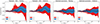 |
Fig. 3. Comparison between the Takahashi et al. (2012) HALOFIT parameters and the new optimised results (HALOFIT+), with the bands giving the 1 and 2σ errors, where we assume that the result of EUCLIDEMULATOR2 is the truth. For both training and validation we use 200 cosmologies and 100 values of k. The dashed horizontal lines indicate an error of ±1%. The new parameters dramatically reduce the errors, particularly for k ≳ 10−1 h Mpc−1. |
5. Corrections to HALOFIT
Up to this point, we have not modified the functional form of HALOFIT. Instead, we have made two major improvements. First, we have increased its speed by removing the requirement to run a root-finding algorithm on integrals of the power spectrum, and having to compute derivatives of the result, by producing concise and accurate symbolic expressions for the output of this procedure. Second, by re-optimising the coefficients appearing in the HALOFIT formalism, we have improved the accuracy of the method, with root mean squared errors of better than 2%. In this section, we provide a correction to the functional form of HALOFIT that will allow us to obtain sub-percent level errors.
We parameterise this additional term as
 (39)
(39)
where we expect that A ≪ 1 (we need to provide at most a correction at the level of a few percent) and that A → 0 as k → 0 so that the linear power spectrum is realised on large scales.
To find an expression for A, we again generated training and validation data on Latin hypercubes, using different seeds to those used in the previous sections but the same parameters. We again chose to sample 200 cosmologies for both training and validation and use 100 logarithmically spaced k values between 9 × 10⁻³ and 9 h Mpc−1. We computed the HALOFIT+ prediction using the analytic expressions for kσ, neff and C obtained in Sect. 3, the analytic approximation to the linear matter power spectrum of Bartlett et al. (2024), and the parameters found in Sect. 4. We divided the output of EUCLIDEMULATOR2 by this quantity and subtracted 1 to obtain the target values of A. To make our target 𝒪(1), we chose to fit for 10A rather than A.
Again, we used OPERON to obtain candidate analytic expressions. We found that a value of ϵ = 10−3 is appropriate and ran for 24 h using a single node with 128 cores, optimising root mean squared error and model length. Since we do not want very complex expressions, we limited the maximum model length to 70. All candidate expressions are comprised of standard arithmetic operations (addition, subtraction, multiplication, division), as well as the natural logarithm, square root, cosine, power and analytic quotient operator ( ). We found that using y = k/kσ enabled a more efficient search than using k directly, so we attempted to find A as a function of y, kσ, neff, C, a and the cosmological parameters.
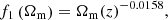
In Fig. 4 we plot the Pareto front of solutions obtained by OPERON which approximate A. We see that for model lengths up to approximately 25, the training and validation losses are approximately equal. Beyond this point, although both losses continue to improve, the rate of improvement decreases for the validation loss, until it stalls at a model length of 44, suggesting a degree of overfitting beyond this point. We therefore chose this function as our approximation to A, which, after merging superfluous constants in the expression, is
![Mathematical equation: $$ \begin{aligned} A&\approx - \frac{d_0}{\sqrt{1 + \left( d_1 { y} \right)^{-d_2 C}}} \Biggl [ { y} - \frac{d_3 \left({ y} - d_4 n_{\rm s} \right)}{\sqrt{\left({ y} - d_5 \log \left( d_6 C\right)\right)^2 + d_7}} \nonumber \\&\quad + \frac{d_8 n_{\rm eff}}{\sqrt{ \left( d_{9}^2 + \sigma _8^2 \right) \left( \left( d_{10} { y} - \cos \left( d_{11} n_{\rm eff} \right) \right)^2 + 1 \right)}} \nonumber \\&\quad + \frac{\left( d_{12} + d_{13} n_{\rm eff} - d_{14} C - d_{15} { y} \right) \left( d_{16} n_{\rm eff} + d_{17} { y} + \cos \left( d_{18} n_{\rm eff} \right)\right)}{\sqrt{{ y}^2 + d_{19}}} \Biggl ], \end{aligned} $$](/articles/aa/full_html/2024/06/aa49854-24/aa49854-24-eq45.gif) (40)
(40)
 |
Fig. 4. Pareto front of solutions found by OPERON to approximate the difference between the nonlinear matter power spectrum and the prediction of HALOFIT. Each point on the red line represents the function with the best mean squared error on the training set for a given model length, whereas the blue curve shows the same loss for these functions evaluated on the validation set. We choose to use the model of length 44, as indicated by the vertical dotted line. |
where the parameters, {di}, are tabulated in Table 2. For the remainder of the paper, we refer to the combination of this correction to HALOFIT model with parameters given by Sect. 4 as SYREN-HALOFIT, the primary product of this work.
Upon inspecting Eq. (40), one notices that, although we allowed the expression to depend on all of the cosmological parameters, the only parameters which appear beyond the standard halofit variables are ns and σ8. It is perhaps unsurprising that these are the two most important variables given that they characterise the slope and normalisation of the initial power spectrum, although it is interesting to find that no other variables are required.
We note that OPERON provided an additional constant offset for Eq. (40), but this is much smaller than the values of A produced, so we ignore it. In fact, this is justified because the leading order term of Eq. (40) as y → 0 is 𝒪(yd2C/2) which, given that d2 > 0 and C > 0 for all cosmologies considered, tends to 0 as y → 0. Hence Eq. (40) does not produce any correction to HALOFIT on large scales, which is desirable as we know linear theory should hold for small k, and this is already the limiting behaviour of HALOFIT+. Keeping the constant offset would not allow this to hold exactly. This demonstrates the advantage of a symbolic expression for P(k) over numerical emulators: the extrapolation behaviour beyond the range of the training data is clear and can be controlled, so we can ensure that the model behaves as desired.
We plot the fractional differences between the nonlinear power spectrum produced by EUCLIDEMULATOR2 and that from SYREN-HALOFIT in Fig. 5. The errors are now reduced to a root mean squared fractional error of 0.9% and 1.0% for the training and validation sets, respectively, and a mean absolute fractional error of 0.7%.
 |
Fig. 5. Distribution of fractional differences between EUCLIDEMULATOR2 and the prediction from HALOFIT plus the correction given in Eq. (40) (SYREN-HALOFIT). For ease of comparison, the range of the y axis is the same as Fig. 3. The bands give the 1 and 2σ values, and we find that the root mean squared fractional error is 0.9% and 1.0% for training and validation, respectively. |
When compared to Fig. 3, we see that the correction predominantly adjusts the prediction at large k, with the two-halo regime being almost unaffected. This can be observed in Fig. 6, where we plot the predictions from EUCLIDEMULATOR2, the BACCO (Angulo et al. 2021) emulator, HMCODE, and the three versions of HALOFIT considered in this work (the parameters of Takahashi et al. (2012); HALOFIT+; and SYREN-HALOFIT) for the Planck 2018 cosmology (Planck Collaboration VI 2020) at a redshift of 1.0. From the central panel, we see that the uncorrected HALOFIT implementation leaves a slowly-varying residual of a few percent with respect to EUCLIDEMULATOR2, which is due to an incorrect prediction from HALOFIT on small scales. The correction given in Eq. (40) fits this residual, but tends to zero for small k, as discussed above. We find that the maximum fractional difference between SYREN-HALOFIT and EUCLIDEMULATOR2 in Fig. 6 is 1.3% which, for context, is only 0.3% greater than the maximum absolute difference between EUCLIDEMULATOR2 and the BACCO emulator.
 |
Fig. 6. Matter power spectrum predictions at redshift 1.0 for the Planck 2018 cosmology (Planck Collaboration VI 2020). We compare the linear theory prediction to that produced by HALOFIT with the parameters of Takahashi et al. (2012); HMCODE as described by Mead et al. (2021); the HALOFIT implementation presented in this work both with (SYREN-HALOFIT) and without (HALOFIT+) the correction given by Eq. (40); EUCLIDEMULATOR2; and the BACCO emulator. The top panel shows the predicted power spectrum and the lower two panels give the residuals with respect to the HALOFIT version of this work without the correction of Eq. (40) and EUCLIDEMULATOR2. |
We note that we have chosen not to further re-optimise the coefficients in Eqs. (29)–(38) in conjunction with the parameters of Eq. (40). Small gains in accuracy are potentially possible under this procedure, but we choose not to perform this optimisation to make the correction factor easier to use (one does not need to use different HALOFIT coefficients if one chooses to switch on the correction factor).
6. Emulator peformance
6.1. Accuracy
When optimising the parameters of HALOFIT in Sect. 4 and obtaining the symbolic correction in Sect. 5, we always compared to EUCLIDEMULATOR2, since this provided a computationally convenient method for generating large numbers of power spectra at arbitrary redshifts. However, it is important to verify that our expressions are accurate when compared to the true outputs of N-body simulations, so in this section we do this for both our expressions and other approaches from the literature.
To make this comparison, we compared our predictions to those from the QUIJOTE suite of simulations (Villaescusa-Navarro et al. 2020). These simulations were run within a cubic box of side length L = 1 h−1 Gpc and N3 = 5123 particles using the GADGET-III code (Springel 2005). We analysed the results at the fiducial cosmology which has the Planck 2018 cosmological parameters (Planck Collaboration VI 2020): Ωm = 0.3175, Ωb = 0.049, h = 0.6711, ns = 0.9624, σ8 = 0.834. We chose this suite since there exist 15 000 simulations at this resolution and cosmology, each with different initial conditions. Thus we can average over the large number of simulations so that we suppress cosmic variance and extract the cosmic mean. The matter power spectrum was extracted at 77 values of k in the range 0.02 − 0.5 h−1 Mpc−1; this k range was chosen since, for larger k, the mean from the 15 000 simulations at this resolution deviates by more than few percent of that obtained from the mean of the 100 simulations ran at higher resolutions (N3 = 10243), suggesting a lack of convergence on those scales.
In Fig. 7 we plot the fractional residuals between the various emulators and the QUIJOTE power spectrum at redshifts 0 and 1. As before, we find that the parameters of Takahashi et al. (2012) results in deviations much larger than a percent for a wide range of k. Although HMCODE performs well at z = 0, we find that it performs worse than HALOFIT at intermediate values of k at a redshift of 1. When using our optimised parameters, we find that the fractional error on the HALOFIT+ prediction is much smaller, although the correction of Eq. (40) is needed to have a percent-level error for larger values of k. We find that the numerical emulators are of comparable accuracy to SYREN-HALOFIT.
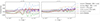 |
Fig. 7. Fractional error on the nonlinear power spectrum as a function of wavenumber, k, for various emulators at redshifts 0 and 1. We take the truth to be the average over all QUIJOTE simulations considered. For reference, the dashed horizontal lines indicate a ±1% error band. |
All the HALOFIT predictions (including HALOFIT+ and SYREN-HALOFIT) have oscillatory residuals with respect to the truth around the BAO scale. This suggests that the HALOFIT model cannot sufficiently capture the changes to the BAO features which occur when moving from the linear to the nonlinear power spectrum. Thus, future work should be dedicated to improving the HALOFIT formalism to better capture these oscillations. We note that the residuals of the EUCLIDEMULATOR2 contain much higher frequency oscillations than HALOFIT, suggesting that these are due to numerical noise. These are not present in the analytic expressions, since it is difficult to produce such high frequency oscillations at moderate model lengths with the basis functions provided.
6.2. Speed
As argued in earlier sections, by avoiding the root-finding procedure and many integrals which need to be performed for the standard implementation of HALOFIT, we expect that our method should be significantly faster, as well as more accurate. We compare our approximations (with and without the correction of Sect. 5) to the Takahashi et al. (2012) version of HALOFIT and HMCODE, as described in Mead et al. (2021), which we compute using CAMB; EUCLIDEMULATOR2 (Euclid Collaboration 2021); and the BACCO emulator (Angulo et al. 2021).
To assess the run time, we evaluated the nonlinear power spectrum at redshift 1 for the Planck 2018 cosmology (Planck Collaboration VI 2020) 103 times on an Intel Xeon E5-4650 CPU, and report the mean execution time per evaluation. We used 200 logarithmically spaced values of k in the range k = 9 × 10⁻³ − 4.9 h Mpc−1. We note that CAMB and EUCLIDEMULATOR2 require As, whereas the other methods require σ8. If one had one variable and needed the other, traditional analyses would require one to run a Boltzmann solver to obtain the linear power spectrum to convert between the two. Although Bartlett et al. (2024) produced an analytic expression for this conversion which can bypass this requirement, since it is application-dependent whether one starts with As or σ8, we assume that we have available whichever of As or σ8 is required by the emulator in question. For the implementation of the expressions obtained in this paper, we used the linear matter power spectrum approximation of Bartlett et al. (2024) and considered both a PYTHON3 and a FORTRAN90 implementation, highlighting the simplicity of exporting symbolic expressions to a different programming language. In our PYTHON3 implementation we used the COLOSSUS (Diemer 2018) package to evaluate the Eisenstein & Hu (1998) transfer function, whereas this was rewritten for the FORTRAN90 implementation.
The results of this timing test are shown in Fig. 8, where we plot the accuracy – computed as the maximum (between z = 0 and 1) of the root mean squared fractional errors between the emulator and QUIJOTE for the k range used in Sect. 6.1 – against the run time. We see that both the corrected (SYREN-HALOFIT) and uncorrected (HALOFIT+) versions of HALOFIT presented in this work require less than 1.5 ms to evaluate in PYTHON3 and just 200 μs in FORTRAN90, which is significantly shorter than the other methods. The compilation of the FORTRAN90 version, itself rapid, only needs to be done once for all further applications of the emulator. We find that our methods, although symbolic like the implementations of HALOFIT and HMCODE in CAMB, are a factor of 2350 and 3170 times faster, respectively, when using our FORTRAN90 code. Given the short expressions, our method is also faster to evaluate than the BACCO emulator by a factor of 64.
 |
Fig. 8. Maximum (between z = 0 and 1) root mean squared fractional error with respect to the QUIJOTE power spectra against run time for various nonlinear power spectrum emulators. The run time of EUCLIDEMULATOR2 is dominated by the Boltzmann code CLASS; the emulation run time is comparable to that of the BACCO emulator, as indicated by the unfilled cross. Our results are orders of magnitude faster than the other methods, with our best method – SYREN-HALOFIT – achieving even greater accuracy than the numerical emulators. |
A somewhat surprising feature of Fig. 8 is the long runtime of EUCLIDEMULATOR2; our methods are 2680 times faster than this approach. This becomes less surprising when one realises that EUCLIDEMULATOR2 only predicts the ratio between the nonlinear and linear matter power spectrum (boost) and it relies on using a Boltzmann solver – in this case CLASS (Blas et al. 2011) – to evaluate the linear power spectrum. We find that the emulation of the boost takes an average of 13 ms (as indicated by the hollow cross in Fig. 8) which, although much smaller than the total runtime, is still 62 times slower than the symbolic methods we developed.
7. Conclusions
In this paper we have used symbolic regression to eliminate two significant limitations of previous symbolic approximations of the nonlinear matter power spectrum, namely that they were not competitive in terms of speed or accuracy compared to numerical emulators. Our approach is to use symbolic regression with genetic programming as implemented by OPERON to improve the well-established HALOFIT approach in three ways:
-
By providing symbolic expressions for all variables appearing in HALOFIT, we remove the need to perform integrals, run root-finding algorithms or use a Boltzmann solver. This results in an increase of a factor of 2350 in speed, and is 2680 and 64 times faster than EUCLIDEMULATOR2 and the BACCO emulator, respectively. These expressions are given in Eqs. (25)–(27).
-
We provide updated HALOFIT parameters to fit a wide range of cosmologies between redshifts 0 and 3 designed to provide the best possible predictions for cosmological parameters of interest for present-day studies. We find that this improves the accuracy by approximately a factor of two for k = 9 × 10⁻³ − 9 h Mpc−1. The updated coefficients are given in Eqs. (29)–(38).
-
We obtain a simple analytic expression to multiply the newly optimised HALOFIT prediction by, which reduces the mean squared error to 1%, providing comparable accuracy to state of the art numerical emulators. This expression is given in Eqs. (39) and (40).
In this work we have restricted our attention to the standard ΛCDM model, with zero neutrino mass and a constant equation of state for dark energy. Given that current and upgoing cosmological surveys such as Euclid (Laureijs et al. 2011), LSST (LSST Science Collaboration 2009), DESI (DESI Collaboration 2016) and WFIRST (Akeson et al. 2019) will be able to probe the nature of dark energy and the neutrino mass, in future work we will extend our formalism for both the linear and nonlinear matter power spectrum to include non-trivial equations of states and a non-zero neutrino mass. We also note that in this work we have not attempted to alter the underlying form of HALOFIT, except for multiplying the final prediction by a correction function to obtain SYREN-HALOFIT. When inspecting these expressions (Eqs. (12), (15) and (16)) and in particular the equations for the parameters which enter them (Eqs. (29)–(38)), one may suppose that more accurate fits could be obtained by using symbolic regression to find a fundamentally more accurate parameterisation. In particular, by automating the search over candidate models, one could allow these to vary in more complicated manners and allow a wider range of cosmological parameters to appear in these expressions. We leave such an investigation to future work.
Accelerating the calculation of important quantities in cosmology does not necessarily require the use of numerical emulators such as neural networks, despite their increasing popularity. We have demonstrated here and in Bartlett et al. (2024) that the more traditional “fitting function” approach – augmented by symbolic regression – can achieve similar (percent level) accuracy but with shorter evaluation times than these emulators. The interpretability, clear extrapolation behaviour, portability, and longevity of these analytic approximations bode well for their future in cosmological emulation.
Acknowledgments
We thank David Alonso, Anirban Bairagi, Bogdan Burlacu Lukas Kammerer and Gabriel Kronberger for useful inputs, comments and suggestions. DJB is supported by the Simons Collaboration on “Learning the Universe.” BDW acknowledges support from the Simons Foundation and from the DIM-ORIGINS “Infinity Next” project. MZ is supported by STFC. PGF acknowledges support from STFC and the Beecroft Trust. HD is supported by a Royal Society University Research Fellowship (grant no. 211046). We made extensive use of computational resources at the University of Oxford Department of Physics, funded by the John Fell Oxford University Press Research Fund, and at the Institut d’Astrophysique de Paris. Data availability: the data underlying this article will be shared on reasonable request to the corresponding author. We provide PYTHON3 and FORTRAN90 implementations of SYREN-HALOFIT at https://github.com/DeaglanBartlett/symbolic_pofk.
References
- Affenzeller, M., Wagner, S., Winkler, S., & Beham, A. 2009, Genetic Algorithms and Genetic Programming (Chapman and Hall/CRC) [CrossRef] [Google Scholar]
- Akeson, R., Armus, L., Bachelet, E., et al. 2019, ArXiv e-prints [arXiv:1902.05569] [Google Scholar]
- Alestas, G., Kazantzidis, L., & Nesseris, S. 2022, Phys. Rev. D, 106, 103519 [NASA ADS] [CrossRef] [Google Scholar]
- Angulo, R. E., Zennaro, M., Contreras, S., et al. 2021, MNRAS, 507, 5869 [NASA ADS] [CrossRef] [Google Scholar]
- Aricò, G., Angulo, R. E., & Zennaro, M. 2021, ArXiv e-prints [arXiv:2104.14568] [Google Scholar]
- Bardeen, J. M., Bond, J. R., Kaiser, N., & Szalay, A. S. 1986, ApJ, 304, 15 [Google Scholar]
- Bartlett, D. J., Desmond, H., & Ferreira, P. 2023a, IEEE Transactions on Evolutionary Computation, https://doi.org/10.1109/TEVC.2023.3280250 [Google Scholar]
- Bartlett, D. J., Desmond, H., & Ferreira, P. G. 2023b, GECCO ’23 Companion: Proceedings of the Companion Conference on Genetic and Evolutionary Computation, 2402 [Google Scholar]
- Bartlett, D. J., Kammerer, L., Kronberger, G., et al. 2024, A&A, in press, https://doi.org/10.1051/0004-6361/202348811 [Google Scholar]
- Bird, S., Viel, M., & Haehnelt, M. G. 2012, MNRAS, 420, 2551 [Google Scholar]
- Blas, D., Lesgourgues, J., & Tram, T. 2011, J. Cosmol. Astropart. Phys., 2011, 034 [CrossRef] [Google Scholar]
- Burlacu, B. 2023, Proceedings of the Companion Conference on Genetic and Evolutionary Computation, GECCO ’23 Companion (New York: Association for Computing Machinery), 2412 [CrossRef] [Google Scholar]
- Burlacu, B., Kronberger, G., & Kommenda, M. 2020, Proceedings of the 2020 Genetic and Evolutionary Computation Conference Companion, GECCO ’20 (New York: Association for Computing Machinery), 1562 [CrossRef] [Google Scholar]
- Casarini, L., Bonometto, S. A., Tessarotto, E., & Corasaniti, P. S. 2016, J. Cosmol. Astropart. Phys., 2016, 008 [CrossRef] [Google Scholar]
- Cooray, A., & Sheth, R. 2002, Phys. Rep., 372, 1 [Google Scholar]
- Delgado, A. M., Wadekar, D., Hadzhiyska, B., et al. 2022, MNRAS, 515, 2733 [NASA ADS] [CrossRef] [Google Scholar]
- DESI Collaboration (Aghamousa, A., et al.) 2016, ArXiv e-prints [arXiv:1611.00036] [Google Scholar]
- Desmond, H., Bartlett, D. J., & Ferreira, P. G. 2023, MNRAS, 521, 1817 [NASA ADS] [CrossRef] [Google Scholar]
- Diemer, B. 2018, ApJS, 239, 35 [NASA ADS] [CrossRef] [Google Scholar]
- Eisenstein, D. J., & Hu, W. 1998, ApJ, 496, 605 [Google Scholar]
- Eisenstein, D. J., & Hu, W. 1999, ApJ, 511, 5 [Google Scholar]
- Euclid Collaboration (Knabenhans, M., et al.) 2021, MNRAS, 505, 2840 [NASA ADS] [CrossRef] [Google Scholar]
- Fendt, W. A., & Wandelt, B. D. 2007a, arXiv e-prints [arXiv:0712.0194] [Google Scholar]
- Fendt, W. A., & Wandelt, B. D. 2007b, ApJ, 654, 2 [NASA ADS] [CrossRef] [Google Scholar]
- Goldberg, D. E. 1989, Genetic Algorithms in Search, Optimization and Machine Learning, 1st edn. (USA: Addison-Wesley Longman Publishing Co., Inc.) [Google Scholar]
- Hahn, O., List, F., & Porqueres, N. 2023, J. Cosmol. Astropart. Phys., submitted [arXiv:2311.03291] [Google Scholar]
- Hajian, A. 2007, Phys. Rev. D, 75, 083525 [NASA ADS] [CrossRef] [Google Scholar]
- Hamilton, A. J. S., Kumar, P., Lu, E., & Matthews, A. 1991, ApJ, 374, L1 [NASA ADS] [CrossRef] [Google Scholar]
- Heitmann, K., Higdon, D., White, M., et al. 2009, ApJ, 705, 156 [Google Scholar]
- Heitmann, K., White, M., Wagner, C., Habib, S., & Higdon, D. 2010, ApJ, 715, 104 [Google Scholar]
- Heitmann, K., Lawrence, E., Kwan, J., Habib, S., & Higdon, D. 2014, ApJ, 780, 111 [Google Scholar]
- Kamerkar, A., Nesseris, S., & Pinol, L. 2023, Phys. Rev. D, 108, 043509 [NASA ADS] [CrossRef] [Google Scholar]
- Kingma, D. P., & Ba, J. 2015, in 3rd International Conference on Learning Representations, ICLR 2015, San Diego, CA, USA, May 7–9, 2015, Conference Track Proceedings, eds. Y. LeCun, & Y. Bengio [Google Scholar]
- Koksbang, S. M. 2023a, Phys. Rev. D, 107, 103522 [CrossRef] [Google Scholar]
- Koksbang, S. M. 2023b, Phys. Rev. D, 108, 043539 [NASA ADS] [CrossRef] [Google Scholar]
- Koksbang, S. M. 2023c, Phys. Rev. Lett., 130, 201003 [NASA ADS] [CrossRef] [Google Scholar]
- Komatsu, E., Dunkley, J., Nolta, M. R., et al. 2009, ApJS, 180, 330 [NASA ADS] [CrossRef] [Google Scholar]
- Komatsu, E., Smith, K. M., Dunkley, J., et al. 2011, ApJS, 192, 18 [Google Scholar]
- Kommenda, M., Burlacu, B., Kronberger, G., & Affenzeller, M. 2020, Genet. Program. Evol. Mach., 21, 471 [CrossRef] [Google Scholar]
- La Cava, W., Orzechowski, P., Burlacu, B., et al. 2021, ArXiv e-prints [arXiv:2107.14351] [Google Scholar]
- Laumanns, M., Thiele, L., Deb, K., & Zitzler, E. 2002, Evol. Comput., 10, 263 [CrossRef] [Google Scholar]
- Laureijs, R., Amiaux, J., Arduini, S., et al. 2011, ArXiv e-prints [arXiv:1110.3193] [Google Scholar]
- Lawrence, E., Heitmann, K., White, M., et al. 2010, ApJ, 713, 1322 [Google Scholar]
- Lemos, P., Jeffrey, N., Cranmer, M., Ho, S., & Battaglia, P. 2023, Mach. Learn.: Sci. Technol., 4, 045002 [NASA ADS] [CrossRef] [Google Scholar]
- Levenberg, K. 1944, Quart. Appl. Math., 2, 164 [Google Scholar]
- Lewis, A., Challinor, A., & Lasenby, A. 2000, ApJ, 538, 473 [Google Scholar]
- Lodha, K., Pinol, L., Nesseris, S., et al. 2024, MNRAS, stae803 [Google Scholar]
- LSST Science Collaboration (Abell, P. A., et al.) 2009, ArXiv e-prints [arXiv:0912.0201] [Google Scholar]
- Ma, C.-P., & Fry, J. N. 2000, ApJ, 543, 503 [Google Scholar]
- Marquardt, D. W. 1963, J. Soc. Indust. Appl. Math., 11, 431 [CrossRef] [Google Scholar]
- Mead, A. J., Peacock, J. A., Heymans, C., Joudaki, S., & Heavens, A. F. 2015, MNRAS, 454, 1958 [NASA ADS] [CrossRef] [Google Scholar]
- Mead, A. J., Heymans, C., Lombriser, L., et al. 2016, MNRAS, 459, 1468 [Google Scholar]
- Mead, A. J., Brieden, S., Tröster, T., & Heymans, C. 2021, MNRAS, 502, 1401 [Google Scholar]
- Miniati, F., & Gregori, G. 2022, Sci. Rep., 12, 11709 [NASA ADS] [CrossRef] [Google Scholar]
- Mootoovaloo, A., Jaffe, A. H., Heavens, A. F., & Leclercq, F. 2022, Astron. Comput., 38, 100508 [NASA ADS] [CrossRef] [Google Scholar]
- Orjuela-Quintana, J. B., Nesseris, S., & Cardona, W. 2023, Phys. Rev. D, 107, 083520 [CrossRef] [Google Scholar]
- Orjuela-Quintana, J. B., Nesseris, S., & Sapone, D. 2024, Phys. Rev. D, 109, 063511 [NASA ADS] [CrossRef] [Google Scholar]
- Peacock, J. A., & Dodds, S. J. 1996, MNRAS, 280, L19 [NASA ADS] [CrossRef] [Google Scholar]
- Planck Collaboration VI. 2020, A&A, 641, A6 [NASA ADS] [CrossRef] [EDP Sciences] [Google Scholar]
- Russeil, E., Ishida, E. E. O., Le Montagner, R., Peloton, J., & Moller, A. 2022, ArXiv e-prints [arXiv:2211.10987] [Google Scholar]
- Russeil, E., Olivetti de França, F., Malanchev, K., et al. 2024, ArXiv e-prints [arXiv:2402.04298] [Google Scholar]
- Seljak, U. 2000, MNRAS, 318, 203 [Google Scholar]
- Smith, R. E., Peacock, J. A., Jenkins, A., et al. 2003, MNRAS, 341, 1311 [Google Scholar]
- Sousa, T., Bartlett, D. J., Desmond, H., & Ferreira, P. G. 2024, Phys. Rev. D, 109, 083524 [NASA ADS] [CrossRef] [Google Scholar]
- Spergel, D. N., Verde, L., Peiris, H. V., et al. 2003, ApJS, 148, 175 [Google Scholar]
- Spergel, D. N., Bean, R., Doré, O., et al. 2007, ApJS, 170, 377 [NASA ADS] [CrossRef] [Google Scholar]
- Springel, V. 2005, MNRAS, 364, 1105 [Google Scholar]
- Spurio Mancini, A., Piras, D., Alsing, J., Joachimi, B., & Hobson, M. P. 2022, MNRAS, 511, 1771 [NASA ADS] [CrossRef] [Google Scholar]
- Takahashi, R., Sato, M., Nishimichi, T., Taruya, A., & Oguri, M. 2012, ApJ, 761, 152 [Google Scholar]
- Taylor, P. L., Kitching, T. D., & McEwen, J. D. 2018, Phys. Rev. D, 98, 043532 [Google Scholar]
- Turing, A. M. 1950, Mind, LIX, 433 [CrossRef] [Google Scholar]
- Villaescusa-Navarro, F., Hahn, C., Massara, E., et al. 2020, ApJS, 250, 2 [CrossRef] [Google Scholar]
- Wadekar, D., Thiele, L., Hill, J. C., et al. 2023, MNRAS, 522, 2628 [NASA ADS] [CrossRef] [Google Scholar]
- Winther, H. A., Casas, S., Baldi, M., et al. 2019, Phys. Rev. D, 100, 123540 [CrossRef] [Google Scholar]
- Zennaro, M., Angulo, R. E., Pellejero-Ibáñez, M., et al. 2023, MNRAS, 524, 2407 [Google Scholar]
All Tables
Range of cosmological parameters and redshift considered when constructing our analytic emulators.
All Figures
|
Fig. 1. Pareto front of solutions found with OPERON for kσ (left; Eq. (7)), neff (centre; Eq. (9)) and C (right; Eq. (10)) over the range of cosmologies and redshifts considered. We plot the Pareto fronts for the training and validation data separately, indicating the lengths of our preferred models with vertical dotted lines. |
| In the text | |
|
Fig. 2. Predicted values (upper) and fractional errors (lower) for kσ (left; Eq. (7)), neff (centre; Eq. (9)) and C (right; Eq. (10)) plotted against their true values, using the results in Eqs. (25)–(27), respectively. The errors are almost always within 2% for kσ, 0.5% for neff and 1% for C. |
| In the text | |
|
Fig. 3. Comparison between the Takahashi et al. (2012) HALOFIT parameters and the new optimised results (HALOFIT+), with the bands giving the 1 and 2σ errors, where we assume that the result of EUCLIDEMULATOR2 is the truth. For both training and validation we use 200 cosmologies and 100 values of k. The dashed horizontal lines indicate an error of ±1%. The new parameters dramatically reduce the errors, particularly for k ≳ 10−1 h Mpc−1. |
| In the text | |
|
Fig. 4. Pareto front of solutions found by OPERON to approximate the difference between the nonlinear matter power spectrum and the prediction of HALOFIT. Each point on the red line represents the function with the best mean squared error on the training set for a given model length, whereas the blue curve shows the same loss for these functions evaluated on the validation set. We choose to use the model of length 44, as indicated by the vertical dotted line. |
| In the text | |
|
Fig. 5. Distribution of fractional differences between EUCLIDEMULATOR2 and the prediction from HALOFIT plus the correction given in Eq. (40) (SYREN-HALOFIT). For ease of comparison, the range of the y axis is the same as Fig. 3. The bands give the 1 and 2σ values, and we find that the root mean squared fractional error is 0.9% and 1.0% for training and validation, respectively. |
| In the text | |
|
Fig. 6. Matter power spectrum predictions at redshift 1.0 for the Planck 2018 cosmology (Planck Collaboration VI 2020). We compare the linear theory prediction to that produced by HALOFIT with the parameters of Takahashi et al. (2012); HMCODE as described by Mead et al. (2021); the HALOFIT implementation presented in this work both with (SYREN-HALOFIT) and without (HALOFIT+) the correction given by Eq. (40); EUCLIDEMULATOR2; and the BACCO emulator. The top panel shows the predicted power spectrum and the lower two panels give the residuals with respect to the HALOFIT version of this work without the correction of Eq. (40) and EUCLIDEMULATOR2. |
| In the text | |
|
Fig. 7. Fractional error on the nonlinear power spectrum as a function of wavenumber, k, for various emulators at redshifts 0 and 1. We take the truth to be the average over all QUIJOTE simulations considered. For reference, the dashed horizontal lines indicate a ±1% error band. |
| In the text | |
|
Fig. 8. Maximum (between z = 0 and 1) root mean squared fractional error with respect to the QUIJOTE power spectra against run time for various nonlinear power spectrum emulators. The run time of EUCLIDEMULATOR2 is dominated by the Boltzmann code CLASS; the emulation run time is comparable to that of the BACCO emulator, as indicated by the unfilled cross. Our results are orders of magnitude faster than the other methods, with our best method – SYREN-HALOFIT – achieving even greater accuracy than the numerical emulators. |
| In the text | |
Current usage metrics show cumulative count of Article Views (full-text article views including HTML views, PDF and ePub downloads, according to the available data) and Abstracts Views on Vision4Press platform.
Data correspond to usage on the plateform after 2015. The current usage metrics is available 48-96 hours after online publication and is updated daily on week days.
Initial download of the metrics may take a while.