| Issue |
A&A
Volume 690, October 2024
|
|
|---|---|---|
| Article Number | A236 | |
| Number of page(s) | 16 | |
| Section | Cosmology (including clusters of galaxies) | |
| DOI | https://doi.org/10.1051/0004-6361/202451343 | |
| Published online | 11 October 2024 | |
PineTree: A generative, fast, and differentiable halo model for wide-field galaxy surveys
1
Sorbonne Université, CNRS, UMR 7095, Institut d’Astrophysique de Paris,
98 bis boulevard Arago,
75014
Paris,
France
2
The Oskar Klein Centre, Department of Physics, Stockholm University, Albanova University Center,
SE 106 91
Stockholm,
Sweden
★ Corresponding author; This email address is being protected from spambots. You need JavaScript enabled to view it.
Received:
2
July
2024
Accepted:
1
August
2024
Abstract
Context. Accurate mock halo catalogues are indispensable data products for developing and validating cosmological inference pipelines. A major challenge in generating mock catalogues is modelling the halo or galaxy bias, which is the mapping from matter density to dark matter halos or observable galaxies. To this end, N-body codes produce state-of-the-art catalogues. However, generating large numbers of these N-body simulations for big volumes, especially if magnetohydrodynamics are included, requires significant computational time.
Aims. We introduce and benchmark a differentiable and physics-informed neural network that can generate mock halo catalogues of comparable quality to those obtained from full N-body codes. The model design is computationally efficient for the training procedure and the production of large mock catalogue suites.
Methods. We present a neural network, relying only on 18 to 34 trainable parameters, that produces halo catalogues from dark matter overdensity fields. The reduction in network weights was realised through incorporating symmetries motivated by first principles into our model architecture. We trained our model using dark-matter-only N-body simulations across different resolutions, redshifts, and mass bins. We validated the final mock catalogues by comparing them to N-body halo catalogues using different N-point correlation functions.
Results. Our model produces mock halo catalogues consistent with the reference simulations, showing that this novel network is a promising way to generate mock data for upcoming wide-field surveys due to its computational efficiency. Moreover, we find that the network can be trained on approximate overdensity fields to reduce the computational cost further. We also present how the trained network parameters can be interpreted to give insights into the physics of structure formation. Finally, we discuss the current limitations of our model as well as more general requirements and pitfalls of approximate halo mock generation that became evident from this study.
Key words: methods: statistical / galaxies: abundances / galaxies: halos / galaxies: statistics / dark matter / large-scale structure of Universe
© The Authors 2024
 Open Access article, published by EDP Sciences, under the terms of the Creative Commons Attribution License (https://creativecommons.org/licenses/by/4.0), which permits unrestricted use, distribution, and reproduction in any medium, provided the original work is properly cited.
This article is published in open access under the Subscribe to Open model. This email address is being protected from spambots. You need JavaScript enabled to view it. to support open access publication.
1 Introduction
Modern surveys like Euclid (Laureijs et al. 2011; Euclid Collaboration 2024b), DESI (DESI Collaboration 2016), LSST (LSST Science Collaboration 2009), PFS (Takada et al. 2014), SKA (Braun et al. 2019; Weltman et al. 2020), WFIRST (Green et al. 2012), and SPHEREx (Doré et al. 2014) are transforming cosmology into a data-driven research field with their unprecedented survey volume and instrument sensitivity. The constraints on cosmological parameters will shift from a noise-dominated regime to a systematics-dominated one. Thus, progress in the field will critically depend on our ability to model the data with ever-increasing accuracy and precision.
To this end, simulated observations or mock data are essential data products for developing new models and cosmological inference pipelines, as is demonstrated by Beyond-2pt Collaboration (2024). Another application utilises mocks to estimate the sample covariance matrix numerically for clustering statistics with the two-point and three-point correlation functions (like Percival et al. 2014). With the advance of machine-learning techniques in recent years, cosmologists have also explored various applications by leveraging simulations to train deep neural networks (e.g. Ravanbakhsh et al. 2017; Fluri et al. 2019; Villanueva-Domingo & Villaescusa-Navarro 2022; Anagnostidis et al. 2022; Perez et al. 2023; Boonkongkird et al. 2023; Jamieson et al. 2023; Legin et al. 2024). Notably, the combination of machine learning with Bayesian statistics known as simulation-based inference (SBI) or implicit likelihood inference (ILI) has established itself as a promising framework in cosmological analysis (Hahn et al. 2023; Ho et al. 2024; Makinen et al. 2022; de Santi et al. 2023).
The state-of-the-art method of generating mock observables involves N-body codes such as Gadget (Springel et al. 2021), Ramses (Teyssier 2002), ENZO, Pkdgrav-3 (an earlier version described by Stadel 2001), and Abacus to trace the evolution of matter over cosmic time. Subsequently, halo finders like Friends-of-friends (Davis et al. 1985), SUBFIND (Springel et al. 2001), HOP (Eisenstein & Hut 1998), AdaptaHOP (Colombi 2013; Aubert et al. 2004), Amiga Halo Finder (Knollmann & Knebe 2009), ASOHF (Planelles & Quilis 2010), and ROCKSTAR (Behroozi et al. 2013) group the particles hierarchically into halos or galaxies. These powerful N-body simulations can be computationally expensive, especially if they aim to cover large survey volumes, include baryonic physics, or explore the effect of different astrophysical and cosmological parameters like Euclid Collaboration (2024a); Villaescusa-Navarro et al. (2020); Nelson et al. (2019); Garrison et al. (2018); Ishiyama et al. (2021). Running these simulations requires millions of CPU hours and petabytes of storage. A growing need for simulation suites with large sets of independent samples aggravates the issue of computational resources. Work done by Blot et al. (2016) shows that more than 5000 independent mock observations are necessary in a Euclid-like setting to estimate the numerical covariance with adequate accuracy for the matter power spectrum. Similarly, the performance of machine-learning methods is directly dependent on the number of available simulations. In situations with sparse training data, deep neural networks are likely to over-fit, and thus may yield biased or overconfident results, as is discussed by Hermans et al. (2021) for ILI algorithms.
Several methods have been proposed to alleviate the reliance on running large sets of high-fidelity N-body simulations. For example, techniques like CARPool (Chartier et al. 2021; Chartier & Wandelt 2021) or ensembling (Hermans et al. 2021) reduce the required number of expensive N-body runs. An alternative approach involves building approximate simulators that are computationally faster than N-body codes, while maintaining sufficient accuracy. Blot et al. (2016) demonstrates that for matter power spectrum analysis in a Euclid-like scenario, the cosmological constraints are substantially weaker with scale cuts of k ≤ 0.2 h Mpc−1, whereas only adopting linear covariance to include smaller scales results in overconfident parameter estimations. This effect will be exacerbated for other summary statistics such as k-th nearest neighbour (Yuan et al. 2023), density-split clustering (Paillas et al. 2023), skew spectrum (Hou et al. 2024), wavelet scattering transforms (Valogiannis et al. 2024; Régaldo-Saint Blancard et al. 2024), cosmic voids (Hamaus et al. 2020; Contarini et al. 2023), or full field-level methods (Jasche & Wandelt 2013; Porqueres et al. 2023; Villaescusa-Navarro et al. 2021; Zhou & Dodelson 2023; Schmidt et al. 2019; Nguyen et al. 2024; Seljak et al. 2017; Jindal et al. 2023; Doeser et al. 2023), since these approaches are shown to be even more sensitive to non-linear and non-Gaussian signals in the data. Therefore, it is crucial to explore approximation methods to produce mocks that accurately capture non-linear effects to smaller scales (k > 0.2 h Mpc−1) as this will ultimately determine how much information and physical insights we shall be able to extract from upcoming surveys (Nguyen et al. 2021, 2024). A vital challenge in generating fast and realistic mock catalogues is to model the link between the matter density field and the resulting galaxies or their host halos, denoted as galaxy or halo bias.
The scope of this paper focuses on constructing dark matter (DM) halos, since around 80% of the total matter is made out of DM, and this hence dominates the dynamics. These halo catalogues are well-founded intermediate data products that can then be transformed into galaxy catalogues through methods such as ‘halo occupation distribution’ (e.g. Jing et al. 1998; Peacock & Smith 2000; Seljak 2000; Yang et al. 2003; Zheng et al. 2005; Yang et al. 2008, 2009; Zehavi et al. 2011, henceforth HOD), ‘subhalo abundance matching’ (e.g. Vale & Ostriker 2004; Behroozi et al. 2010; Moster et al. 2010; Reddick et al. 2013; Chaves-Montero et al. 2016; Lehmann et al. 2017; Stiskalek et al. 2021, hereinafter SHAM), ADDGALS (Wechsler et al. 2022), or semi-analytic models (e.g. Yung et al. 2022a,b).
In this work, we propose a generative and physics-informed neural network that we call PineTree (Physical and interpretable network for tracer emulation), which emulates the halo bias and can sample realistic DM halo catalogues in a computationally efficient way. The subsequent section will briefly review existing mock generation approaches and set the context for our method. We shall then continue to describe the set-up of our model and how it is trained and used to generate mock catalogues in Sects. 3 and 4. This naturally leads to Sect. 5, in which we discuss our results, before we conclude with a summary and outline of follow-up projects and applications.
2 Overview of mock generation frameworks
The first analytical approaches to predict DM halo distributions – namely, the halo mass function, from DM density fields – were pioneered by Kaiser (1984); Bardeen et al. (1986) and later refined (e.g. through works by Bond 1987; Bond et al. 1988; Carlberg & Couchman 1989; Cole & Kaiser 1989; Mo & White 1996; Sheth & Tormen 1999) into the formalism known now as ‘peak background split’. In contrast, an alternative approach based on ‘excursion sets’ (e.g. Schaeffer & Silk 1985, 1988; Kaiser 1988; Cole & Kaiser 1988, 1989; Efstathiou et al. 1988; Efstathiou & Rees 1988; Narayan & White 1988) that was initially formulated by Press & Schechter (1974) as the Press-Schechter formula was developed. It was later extended by Bond et al. (1991) and further improved with the addition of ellipsoidal collapse (Sheth et al. 2001; Sheth & Tormen 2002). Using these physically derived schemes, it is possible as a first approximation to predict the halo mass function and, at the first order, the linear relation between the halo and matter density contrast,
![Mathematical equation: $\[\delta_{\mathrm{h}}=b ~\delta_{\mathrm{m}},\]$](/articles/aa/full_html/2024/10/aa51343-24/aa51343-24-eq1.png) (1)
(1)
with b as a scale-independent bias parameter. δm and δh denote the (dark) matter and halo relative density contrast, respectively.
However, the linear bias is only a valid approximation for the largest cosmological scales as it fails to account for any nonlinear (Kravtsov & Klypin 1999) and scale-dependent (Smith et al. 2007) behaviour. Fry & Gaztanaga (1993) extended the analytical framework to quasi-linear scales through ‘local bias expansion’. The perturbative bias expansion expresses the halo number density (or galaxy number density) as a function of the matter density field and its higher-order derivatives like the tidal field. For an extensive review of the perturbative bias treatment, we refer the reader to Desjacques et al. (2018). Notably, the concept of ‘local-in-matter-density bias’ (Desjacques et al. 2018, hereinafter LIMD bias) has been extended to phenomenological bias models beyond the linear bias such as power-law parametrisations (Cen & Ostriker 1993; de la Torre & Peacock 2013) or other non-linear bias functions (Neyrinck et al. 2014; Repp & Szapudi 2020). The main idea of using LIMD bias models for mock generation is to produce a mean halo density field from a smoothed matter density field and then sample the halo field (e.g. through a Poisson distribution) to get a discrete count field.
Chan et al. (2012); Sheth et al. (2013) show – and this was highlighted again by Bartlett et al. (2024) – that the local bias is insufficient to predict the halo distribution correctly. Here, it is also important to emphasise that phenomenological bias methods need to be validated thoroughly since there is no theoretical guarantee of their accuracy, unlike the perturbative approach. Figure 1 depicts the breakdown of a local biasing scheme as well as the discrepancies in different validation metrics for which we fit the truncated power law (TPL) bias to a gravity-only N-body simulation following (Neyrinck et al. 2014). We show that the calibrated TPL can reproduce the overall halo count distribution of the simulation, effectively validating the one-point statistics. But when comparing the power spectra (two-point correlation) we can see a clear difference between the sampled mock fields and the reference N-body simulation. Bartlett et al. (2024) show that this trend is true for any LIMD bias scheme. Therefore, it is imperative to validate the mocks across different statistical orders, especially if the scientific target is to generate realistic halos on the field level.
So far, we have only discussed methods utilising fast analytic halo bias schemes to generate mocks. An alternative to reduce (considerably) the computational cost is to accelerate the generation of the underlying DM density by approximate gravity solvers. This type of approach, also known as ‘Lagrangian methods’, involves the computation of an approximate matter distribution coupled with a deterministic halo formation prescription (see Monaco 2016 for a more comprehensive review). The first methods of this class such as PINOCCHIO Monaco et al. (2002b,a); Taffoni et al. (2002), PEAK-PATCH (Bond & Myers 1996), and PTHalos (Scoccimarro & Sheth 2002; Manera et al. 2012; Manera et al. 2014) adopted Lagrangian perturbation theory for the density field computation. Later works propose to utilise more accurate gravity solvers based on the particle-mesh scheme such as PMFAST (Merz et al. 2005), FastPM (Feng et al. 2016), COLA (Tassev et al. 2013; Koda et al. 2016; Izard et al. 2016; Ding et al. 2024), and its variants L-PICOLA (Howlett et al. 2015a) and sCOLA (Tassev et al. 2015; Leclercq et al. 2020). One downside of these algorithms is that they rely on Friends-of-friends or other particle-based halo finders, which can result in a computationally intense process when high accuracy is required (see for instance Blot et al. 2019; Monaco 2016). Still, these methods have been readily adopted in combination with HOD or SHAM to generate mock surveys, as is demonstrated by Howlett et al. (2015b); Drinkwater et al. (2010); Kazin et al. (2014); Ferrero et al. (2021).
The natural extension of these approaches is to combine approximate gravity solvers to produce smoothed density fields with simplified bias prescriptions, as has been done by PATCHY (Kitaura et al. 2013), QPM (White et al. 2013), EZmocks (Chuang et al. 2014), and Halogen (Avila et al. 2015). Notably, these methods include a stochastic component to address the stochasticity of halo bias (as discussed by e.g. Pen 1998; Tegmark & Bromley 1999; Dekel & Lahav 1999; Matsubara 1999; Sheth & Lemson 1999; Taruya & Soda 1999; Seljak & Warren 2004; Neyrinck et al. 2005; Hamaus et al. 2010; Baldauf et al. 2013). Despite utilising (local) bias schemes that can be difficult to calibrate, this type of mock generation approach has been successfully applied by Kitaura et al. (2015, 2016); Vakili et al. (2017) to produce large suites of accurate mock catalogues (see also Chuang et al. 2015; Monaco 2016 for a comparison of some of the methods).
In recent years, new techniques for mock generation have been explored to achieve even greater accuracy and computational efficiency. For instance, BAM (Balaguera-Antolínez et al. 2018, 2019, 2023; Kitaura et al. 2022; García-Farieta et al. 2024) proposes a non-parametric bias scheme that samples halos based on the underlying matter density field and its associated cosmic web-type information motivated by Yang et al. (2017); Fisher & Faltenbacher (2017). Meanwhile, Modi et al. (2018); Berger & Stein (2018); Zhang et al. (2019); Piras et al. (2023); Pandey et al. (2023); Pellejero Ibañez et al. (2024) have investigated the use of machine learning as bias emulators, since deep neural networks as universal function approximators are powerful tools to accurately model the non-linear behaviour on small scales. Yet, due to their large and degenerate parameter space, neural networks can be difficult and computationally expensive to set up and train, requiring large amounts of high-fidelity training samples. Moreover, large networks are black-box models that cannot be easily interpreted after training. The following section will introduce our mock generation pipeline, PineTree, which leverages machine-learning techniques to incorporate a stochastic and non-local bias scheme, while maintaining an interpretable and reduced parameter space through a physics-motivated model architecture.
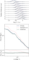 |
Fig. 1 Comparison between using one-point statistics (upper panel) and two-point statistics (lower panel) as validation metrics. The first panel on top shows a kernel density estimate plot of the number of voxels with a given halo count as a function of the underlying DM overdensity. Each line corresponds to the number of halos per voxel, as is indicated by the annotated text on the left. The distributions were produced using a Gaussian kernel with a bandwidth set according to Scott’s rule (Scott 2015). The dark blue, pink, and green curves show the number distribution obtained from N-body simulation, the TPL by Neyrinck et al. (2014), and PineTree respectively. In the bottom panel, we show the mean power spectrum from the generated fields and ratios with respect to the reference N-body simulation. The grey band indicates the 10% deviation threshold. |
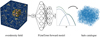 |
Fig. 2 Schematic view of the PineTree pipeline. The following steps are depicted from left to right: the input DM overdensity field was convolved with a rotation-symmetric kernel; a mixture density network computed the distribution parameters of a log-normal mixture distribution with the feature map, ψ halo masses were drawn from the emulated distributions to construct the final halo catalogue. |
3 PineTree
PineTree is a computationally fast and generative model with a minimal set of trainable parameters that takes as an input a gridded DM overdensity field, δm(x), and outputs a halo count overdensity field, δh(x), or halo catalogue, {Mh(x)}, at the same gridding resolution. The mock generation pipeline builds upon the neural physical engine first described by Charnock et al. (2020) and is divided into three parts. The first subsection presents the model architecture and how it differs from conventional machine learning approaches. We then derive the objective function to optimise the model’s parameters and conclude the section by describing how the trained model generates the final halo catalogues (for an overview of the set-up, see the schematic outline in Fig. 2). The code is written in Python and is implemented in the Jax1 framework to enable GPU acceleration. A public version of the source code is hosted on Bitbucket2.
3.1 Network architecture
The network architecture consists of two functional parts: a module to encode the environmental information of the input, and a neural network that approximates the halo mass function. As was mentioned in Sect. 2, we want the network to consider each cell and its surrounding environment. Thus, a network architecture building on a convolutional neural network is the natural choice. Furthermore, we want to encode our prior knowledge into the design of the network; namely, the principal physical forces of structure formation such as gravity are isotropic with regard to the underlying particle distribution. This means that our bias model should a priori be sensitive to neither the specific orientation nor the location of the DM overdensity field when predicting the resulting halo distribution. Hence, the network operation performed on the input field needs to be rotationally and translationally invariant.
3.1.1 Building environment summaries with a convolutional neural network
A standard convolution layer (LeCun et al. 1989) performs a discrete convolution on an input field, I, with a set of kernel weights, ωKernel, and is therefore, by definition, already translation-invariant. In the three-dimensional case, the layer operation with a kernel of size M × N × L can be formally expressed as
![Mathematical equation: $\[\psi_{i j k}=\left(I * \omega^{\text {Kernel }}\right)_{i j k}=\sum_m \sum_n \sum_l I_{i+m, j+n, k+l} ~\omega_{m n l}^{\text {Kernel }}+b \text {, }\]$](/articles/aa/full_html/2024/10/aa51343-24/aa51343-24-eq2.png) (2)
(2)
where the set of indices, {i jk}, relate to a given voxel in the discretised three-dimensional field. In the above equation, the index m runs from – (M − 1)/2 to (M − 1)/2, and in the same way it also runs for the indices n and l to centre the convolutional kernel on the input voxel, Ii jk. In the machine-learning language, the output, ψi jk, is called a feature map and b is denoted as the neural bias parameter that needs to be learned alongside the kernel weights. In the context of this work, however, the term bias will henceforth refer to the DM halo connection, unless stated otherwise. The feature map, ψi jk, can be understood as the compressed information of the overdensity field patch around the central overdensity voxel, δi jk.
To enforce rotational invariance, we applied a multi-pole expansion to the convolutional kernel. Inspired by a conventional multi-pole expansion in which a generic function is decomposed as
![Mathematical equation: $\[f(\theta, \varphi)=\sum_{l=0}^{\infty} \sum_{m=-l}^l C_l^m Y_l^m(\theta, \varphi),\]$](/articles/aa/full_html/2024/10/aa51343-24/aa51343-24-eq3.png) (3)
(3)
with ![Mathematical equation: $\[C_l^m\]$](/articles/aa/full_html/2024/10/aa51343-24/aa51343-24-eq4.png) denoting the constant coefficients and
denoting the constant coefficients and ![Mathematical equation: $\[Y_l^m\]$](/articles/aa/full_html/2024/10/aa51343-24/aa51343-24-eq5.png) the spherical harmonics, we constructed a kernel that has shared weights for kernel positions with
the spherical harmonics, we constructed a kernel that has shared weights for kernel positions with
![Mathematical equation: $\[C_l^m(r, \theta, \varphi)=r ~Y_l^m(\theta, \varphi),\]$](/articles/aa/full_html/2024/10/aa51343-24/aa51343-24-eq6.png) (4)
(4)
where r is the Euclidean distance from the centre of the kernel to the position of the weight. Effectively, we decomposed a convolutional kernel with independent weights into a set of kernels with shared weights, for a given l and m, which is determined by the spherical harmonics; that is, kernel positions with the same ![Mathematical equation: $\[C_l^m(r, \theta, \varphi)\]$](/articles/aa/full_html/2024/10/aa51343-24/aa51343-24-eq7.png) according to Eq. (4). For a rotationally invariant kernel, we only considered the monopole contributions with l = m = 0. The output of the convolution operation then only encodes rotational and translational invariant features. In addition, using this multi-pole expansion approach, the number of independent weights is greatly reduced. For instance, a 5 × 5 × 5 kernel will have only ten independent weights instead of 125. Figure 3 visualises the shared weights of a monopole kernel.
according to Eq. (4). For a rotationally invariant kernel, we only considered the monopole contributions with l = m = 0. The output of the convolution operation then only encodes rotational and translational invariant features. In addition, using this multi-pole expansion approach, the number of independent weights is greatly reduced. For instance, a 5 × 5 × 5 kernel will have only ten independent weights instead of 125. Figure 3 visualises the shared weights of a monopole kernel.
To reduce the parameter space and maximise the computational speed of the model, we adopted a single filter – the monopole kernel – for the convolutional network. Therefore, the feature map, ψi, for a patch around a central overdensity voxel, δi, is presented by a scalar. We note that our public implementation of the method has already been designed to make it possible to include higher-order multi-poles to handle direction-dependent effects (e.g. tidal forces), and potential improvements of utilising a multi-filter convolutional network approach will be explored in future works. Each multi-pole contribution will result in a separate kernel, so in general the output of the convolutional layer can also become a vector, ψ, with each entry corresponding to a distinct feature map associated with a different kernel. The relation to the multi-pole expansion gives us a direct way of interpreting the kernel weights of our model, indicating how important specific spatial locations are for the model prediction. In Sec. 5.4, we shall discuss the interpretation in detail for a trained monopole kernel.
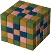 |
Fig. 3 Visualisation of a 5 × 5 × 5 monopole kernel. Identical colours indicate shared weights resulting in a rotationally symmetric pattern. |
3.1.2 The mixture distribution
The second part of the PineTree model is designed to digest the non-local information encoded in ψ and predict a probability function that can then be used to generate halo samples. In this case, we want to model the conditional halo mass function, n(M| {δ}i); that is, the number of expected halos for mass, M, conditioned on an overdensity patch, {δ}i, for the i-th voxel. To ensure that the model can produce flexible and well-defined distributions, we chose a mixture of log-normal distributions, which are also frequently utilised in the machine learning community as density estimation networks. The formal expression of the conditional halo number density then reads:
![Mathematical equation: $\[n\left(M {\mid}\{\delta\}_i\right)=\frac{\bar{N}_i}{V} \sum_{n=1}^{N_{\text {mix }}} \frac{\alpha_{n i}}{M \sqrt{2 \pi \sigma_{n i}^2}} \exp \left[-\frac{\left(\ln M-\mu_{n i}\right)^2}{2 \sigma_{n i}^2}\right],\]$](/articles/aa/full_html/2024/10/aa51343-24/aa51343-24-eq8.png) (5)
(5)
with Nmix as the number of mixture distributions, ![Mathematical equation: $\[\bar{N}_i\]$](/articles/aa/full_html/2024/10/aa51343-24/aa51343-24-eq9.png) the predicted mean halo number for voxel i, and V denoting the voxel volume. The conditioning on the overdensity patch enters through the previously computed feature map, ψi, via the mixture network parameters by:
the predicted mean halo number for voxel i, and V denoting the voxel volume. The conditioning on the overdensity patch enters through the previously computed feature map, ψi, via the mixture network parameters by:
![Mathematical equation: $\[\bar{N}_i=\exp \left[\omega^{\bar{N}} \boldsymbol{\psi}_i+b^{\bar{N}}\right],\]$](/articles/aa/full_html/2024/10/aa51343-24/aa51343-24-eq10.png) (6)
(6)
![Mathematical equation: $\[\alpha_{n i}=\operatorname{softmax}\left(\omega_n^\alpha \boldsymbol{\psi_i}+b_n^\alpha\right),\]$](/articles/aa/full_html/2024/10/aa51343-24/aa51343-24-eq11.png) (7)
(7)
![Mathematical equation: $\[\sigma_{n i}=\exp \left[\omega_n^\sigma \boldsymbol{\psi_i}+b_n^\sigma\right],\]$](/articles/aa/full_html/2024/10/aa51343-24/aa51343-24-eq12.png) (8)
(8)
![Mathematical equation: $\[\mu_{n i}= \begin{cases}\omega_n^\mu \boldsymbol{\psi_i}+b_n^\mu, & \text { if } n=0, \\ \max \left[0, ~\omega_n^\mu \boldsymbol{\psi_i}+b_n^\mu\right]+\mu_{n-1}, & \text { if } n>0.\end{cases}\]$](/articles/aa/full_html/2024/10/aa51343-24/aa51343-24-eq13.png) (9)
(9)
The parameters ![Mathematical equation: $\[\left\{\omega_n^{\bar{N}}, b_n^{\bar{N}}, \omega_n^\alpha, b_n^\alpha, \omega_n^\mu, b_n^\mu, \omega_n^\sigma, b_n^\sigma\right\}\]$](/articles/aa/full_html/2024/10/aa51343-24/aa51343-24-eq14.png) are defined globally for all voxels and the density dependency only enters through ψ. Furthermore, the activation function in Eq. (7) ensures the mixture distribution is properly normalised so that ∑n αni = 1 holds.
are defined globally for all voxels and the density dependency only enters through ψ. Furthermore, the activation function in Eq. (7) ensures the mixture distribution is properly normalised so that ∑n αni = 1 holds.
3.1.3 Final transformations
The final model was put together by first transforming the input overdensity, δm(x), into the logarithmic space log[1 + δm(x)] and then compressing it with the monopole kernel by a convolutional layer. The extracted feature map was subsequently transformed by the ‘softplus’ activation function before finally being chained with the mixture density network. Thus, the full network describes a non-local and non-linear transformation from an overdensity environment patch to a halo number distribution at the environment centre.
It should be highlighted again that, due to the physically motivated design choices, the model only contains a very small parameter set compared to contemporary neural networks, which typically have hundreds of thousands to millions of free parameters. This was realised by utilising the symmetric single-kernel convolutional layer, and the shallow network that translates the feature map, ψ, into the mixture distribution parameters, as is described in Eqs. (6) to (9). For a kernel with size 3 × 3 × 3 and a mixture density network of two components, the PineTree model has a total of 18 parameters, making it suitable to directly infer the model parameters from a given dataset in the context of Bayesian inference or using it as a Bayesian neural network. Section 5.4 discusses the effect of utilising different kernel sizes for which the number of model parameters can increase.
3.2 Loss function
The optimisation problem at hand is to find the best model parameters so that the sampled halo catalogues from our model match the halo catalogues obtained from a N-body halo finder. The evaluation function quantifying the distance of the prediction to the ground truth is called the objective or loss function. In line with the purpose of having an interpretable model, we used a physical likelihood function as the objective function, following the maximum likelihood principle to optimise the model parameters. This approach also enables the easy incorporation of PineTree into existing Bayesian forward modelling frameworks.
The probability distribution of the observed data, d, given the underlying forward model with parameter s is referred to as the likelihood, 𝒫(d |s). The explicit form of the likelihood depends on our assumption about the stochasticity of the observable. The likelihood, in the case of additive noise, can be formally written down by defining the measurement equation,
![Mathematical equation: $\[d=R(s)+n,\]$](/articles/aa/full_html/2024/10/aa51343-24/aa51343-24-eq15.png) (10)
(10)
where the function R(s) denotes the forward model that maps the signal to the expected observation and n denotes an additive noise. Using Eq. (10) and assuming a reasonable distribution for the measurement noise, 𝒫𝒩(n), (often Gaussian or Poissonian), the likelihood can then be written down as
![Mathematical equation: $\[\begin{aligned}\mathcal{P}(d {\mid} s) & =\int \mathcal{P}(d, n {\mid} s) \mathrm{d} n=\int \mathcal{P}(n {\mid} s) \mathcal{P}(d {\mid} n, s) ~\mathrm{d} n \\& =\int \mathcal{P}(n {\mid} s) \delta_D(d-R(s)) ~\mathrm{d} n \\& =\mathcal{P}_{\mathcal{N}}(n=d-R(s)),\end{aligned}\]$](/articles/aa/full_html/2024/10/aa51343-24/aa51343-24-eq16.png) (11)
(11)
with δD denoting the Dirac delta function.
In this work, we assume that the number of halos per mass bin and per voxel is Poisson-distributed:
![Mathematical equation: $\[N_{i, M}^{\text {halo }} \sim \mathcal{P}_{\text {Poisson }}\left(\lambda_{i, M}\right),\]$](/articles/aa/full_html/2024/10/aa51343-24/aa51343-24-eq17.png) (12)
(12)
where λi,M denotes the mean (i.e. the Poisson intensity), and the indices i and M refer to the i-th voxel from the grid and the mass bin, [M, M + ΔM], respectively. Therefore, the mean halo number per voxel for each halo mass bin can be related to the conditional halo number density by
![Mathematical equation: $\[\lambda_{i, M} \equiv\left\langle N_{i, M}\right\rangle=V \int_M^{M+\Delta M} n\left(M {\mid} \delta_i\right) ~\mathrm{d} M,\]$](/articles/aa/full_html/2024/10/aa51343-24/aa51343-24-eq18.png) (13)
(13)
with V denoting the voxel volume. The Poisson log-likelihood for observing ![Mathematical equation: $\[N_{i, M}^{\mathrm{obs}}\]$](/articles/aa/full_html/2024/10/aa51343-24/aa51343-24-eq19.png) is then given by
is then given by
![Mathematical equation: $\[\ln \mathcal{P}_{i, M}\left(d=N_{i, M}^{\mathrm{obs}} \mid \lambda_{i, M}\right)=N_{i, M}^{\mathrm{obs}} \ln \lambda_{i, M}-\ln N_{i, M}^{\mathrm{obs}}!-\lambda_{i, M}.\]$](/articles/aa/full_html/2024/10/aa51343-24/aa51343-24-eq20.png) (14)
(14)
For the optimisation scheme, only the gradient with respect to λi,M is relevant. Therefore, terms depending only on ![Mathematical equation: $\[N_{i, M}^{\mathrm{obs}}\]$](/articles/aa/full_html/2024/10/aa51343-24/aa51343-24-eq21.png) can be discarded, and we shall omit them from now on. Furthermore, we assume that voxels as well as halo mass bins are conditionally independent, yielding the total log-likelihood:
can be discarded, and we shall omit them from now on. Furthermore, we assume that voxels as well as halo mass bins are conditionally independent, yielding the total log-likelihood:
![Mathematical equation: $\[\ln \mathcal{P}\left(N^{\mathrm{obs}} ~{\mid} \lambda\right)=\sum_{i \in \text { voxels }} \sum_{M \epsilon_{\text {bins }}^{\text {mass }}} N_{i, M}^{\text {obs }} \ln \lambda_{i, M}-\lambda_{i, M}.\]$](/articles/aa/full_html/2024/10/aa51343-24/aa51343-24-eq22.png) (15)
(15)
If the halo mass bin width is decreased to the limit ΔM → 0, then the observed number of halos, ![Mathematical equation: $\[N_{i, M}^{\mathrm{obs}}\]$](/articles/aa/full_html/2024/10/aa51343-24/aa51343-24-eq23.png) , can either be one or zero, and the above sums can be rewritten as
, can either be one or zero, and the above sums can be rewritten as
![Mathematical equation: $\[\ln \mathcal{P}\left(N^{\mathrm{obs}} \mid \lambda\right)=\sum_{j \in \text {halos}} \ln \lambda_{i(j), M(j)}-\sum_{i \in \text {voxels}} \int_{M_{\mathrm{th}}}^{\infty} \mathrm{d} M \lambda_{i, M},\]$](/articles/aa/full_html/2024/10/aa51343-24/aa51343-24-eq24.png) (16)
(16)
where the indices i(j) and M(j) correspond to the voxel and mass bin of halo j, respectively. Moreover, Mth denotes the lower mass threshold of the halos in the simulation.
In the optimisation context, following maximum likelihood, the loss function, ℒ, is given by the negative log-likelihood. So, by inserting Eq. (5) and Eq. (13) into Eq. (16), the final expression that needs to be minimised reads:
![Mathematical equation: $\[\begin{aligned}\mathcal{L}= & -\sum_{j \in \text {halos}} \ln \left(\sum_{n=1}^{N_{\text {mix}}} \frac{\tilde{\alpha}_{n i(j)}}{\sqrt{2 \pi \sigma_{n i(j)}^2}} \exp \left[-\frac{\left(\ln M_j-\mu_{n i(j)}\right)^2}{2 \sigma_{n i(j)}^2}\right]\right) \\& \quad+\sum_{i \in \text {voxels}} \int_{M_{t h}}^{\infty} \sum_{n=1}^{N_{\text {mix}}} \frac{\tilde{\alpha}_{n i(j)}}{M \sqrt{2 \pi \sigma_{n i(j)}^2}} \exp \left[-\frac{\left(\ln M-\mu_{n i(j)}\right)^2}{2 \sigma_{n i(j)}^2}\right] \mathrm{d} M \\= & -\sum_{j \in \text {halos}} \ln \left(\sum_{n=1}^{N_{\text {mix}}} \frac{\tilde{\alpha}_{n i(j)}}{\sqrt{2 \pi \sigma_{n i(j)}^2}} \exp \left[-\frac{\left(\ln M_j-\mu_{n i(j)}\right)^2}{2 \sigma_{n i(j)}^2}\right]\right) \\& \quad+\sum_{i \in \text {voxel}} \sum_{n=1}^{N_{\text {mix}}} \frac{\tilde{\alpha}_{n i(j)}}{2} \operatorname{erfc}\left(\frac{\ln \mathrm{M}_{\mathrm{th}}-\mu_{\text {ni}(j)}}{\sqrt{2 \sigma_{n i(j)}^2}}\right).\end{aligned}\]$](/articles/aa/full_html/2024/10/aa51343-24/aa51343-24-eq25.png) (17)
(17)
3.3 Sampling of halos
After obtaining the model parameters with the derived loss function from Eq. (17) and a suitable optimisation scheme, as is described in Sec. 4.2, the PineTree model could then be used to generate mock halo catalogues for a given overdensity field. The sampling procedure was divided into two parts: first, sampling the total number of halos per voxel, and thereafter the mass realisation of each halo. For the number count generation, we need to use the initial assumption that the halos are distributed according to a Poisson distribution (see Eq. (12)). Utilising the additive property of the Poisson distribution and the previous assumption of statistically independent mass bins, we can directly sample the halo count for all mass bins of one voxel rather than separately sampling each mass bin. With regards to the PineTree model, the predicted Poisson intensity per voxel is computed by
![Mathematical equation: $\[\lambda_i=\sum_{M \epsilon_{\text {bins }}^{\text {mass }}} \lambda_{i, M}=\sum_{n=1}^{N_{\text {mix }}} \frac{\tilde{\alpha}_{n i}}{2} \operatorname{erfc}\left(\frac{\ln \mathrm{M}_{\mathrm{th}}-\mu_{\mathrm{ni}}}{\sqrt{2 \sigma_{n i}^2}}\right),\]$](/articles/aa/full_html/2024/10/aa51343-24/aa51343-24-eq26.png) (18)
(18)
which we subsequently use to generate a number realisation, ![Mathematical equation: $\[N_i^{\text {halo }} \curvearrowleft \mathcal{P}_{\text {Poisson }}\left(\lambda_i\right)\]$](/articles/aa/full_html/2024/10/aa51343-24/aa51343-24-eq27.png) . Finally, according to the sampled halo count for each voxel, the individual halo masses are drawn in parallel from the predicted mixture density,
. Finally, according to the sampled halo count for each voxel, the individual halo masses are drawn in parallel from the predicted mixture density,
![Mathematical equation: $\[P(M)=\sum_{n=1}^{N_{\text {mix }}} \frac{\alpha_{n i}}{M \sqrt{2 \pi \sigma_{n i}^2}} \exp \left[-\frac{\left(\ln M-\mu_{n i}\right)^2}{2 \sigma_{n i}^2}\right].\]$](/articles/aa/full_html/2024/10/aa51343-24/aa51343-24-eq28.png) (19)
(19)
We note that the above expression only differs from the conditional halo number density from Eq. (5) by a factor of ![Mathematical equation: $\[\bar{N}_i ~V^{-1}\]$](/articles/aa/full_html/2024/10/aa51343-24/aa51343-24-eq29.png) .
.
4 Training data and configuration
Following the theoretical description of our model in Sec. 3, we detail the technical set-up and parameter choices that led to the results shown in the subsequent section. We first describe the N-body simulations that served as training and validation data before ending the section by reporting the specific model and training configurations that were tested.
Range of tested PineTree configurations.
4.1 Description of the simulation dataset
The N-body simulations were obtained by running a non-public variant of Gadget-2 (Springel 2005); namely, L-Gadget, which is a more computationally efficient version that only simulates collisionless matter. The initial conditions for the N-body simulations were computed by the initial condition generator, GenIC (Nishimichi et al. 2009, 2010; Valageas & Nishimichi 2011). We produced 60 dark-matter-only simulations with different random seeds for the initial conditions using Planck 2018 cosmology (Planck Collaboration VI 2020). To capture large-scale dynamics with good particle resolution for luminous red galaxy halos (e.g. van Uitert, Edo et al. 2015), we ran each simulation with a box size of 5003 h−3 Mpc3 and 5123 particles, which results in a particle mass resolution of 8.16 × 10¹⁰ h−1 M⊙. We set GenIC to use second-order Lagrangian perturbation theory (2LPT) to evolve the initial conditions until a redshift of z = 24, and the successive L-Gadget evolution to z = 0 and z = 1 was executed using a gravity softening of 0.05ℓ, where ℓ = (Vbox/Npart)1/3 is the mean inter-particle separation, with Vbox as the volume of the simulation and Npart denoting the total number of particles. Using the same initial condition seeds as for the L-Gadget simulations, another set of 60 snapshots for each redshift of z ∈ {0, 1} was produced through GenIC only. Henceforth, we refer to this second set of simulations as 2LPT simulations. We used the cloud-in-cell (CIC) interpolation described in Hockney & Eastwood (1981) to obtain the final overdensity fields that were used as inputs for PineTree.
We validated the simulations by comparing the power spectra to the theoretical prediction from the Boltzmann solver CLASS (e.g. Lesgourgues 2011; Blas et al. 2011), which is shown in Appendix A. Finally, we used ROCKSTAR with a linking length of b = 0.28 and minimum halo particle set to 10 particles to produce the corresponding halo catalogues. In this work, we adopted the virial mass definition according to Bryan & Norman (1998), leading to a lower halo mass threshold of 3 × 10¹² h−1 M⊙ for each catalogue. Again, we checked the halo catalogues for potential inconsistencies by comparing the simulated halo mass function to theoretical predictions from Tinker et al. (2008) (see Appendix A).
4.2 Model configuration
In this work, we aim to study the scope of PineTree’s applicability. Thus, we conducted an extensive parameter study and summarised the different configuration choices in Table 1.
For all results presented in the following section, the number of log-normal distributions was always set to two. This was motivated by the intuition on halo mass functions provided by Press & Schechter (1974); Tinker et al. (2008) and insights from the set of N-body simulations (see Sec. 4.1). In addition to the listed configurations in Table 1, we tested further configurations, such as a different number of mixture components. However, these runs did not significantly improve our results and a complete report on the specific settings with their outcome is given in Appendix B.1.
We opted for the gradient-based optimiser Adam by Kingma & Ba (2014) to achieve the optimisation. The learning rate was set to 0.001 for all results shown in this work. Other values and various learning rate schedulers were also tested without notable improvements. We considered the network parameters to have converged when the loss computed on the set of validation simulations saturated. Unless stated otherwise, the 60 simulations were split into a training set comprising 10 simulations and the validation set was made up of 30 different simulations that the model did not see during training. The remaining 20 simulations were used for testing and we shall justify our choice of only utilising 10 simulations for the training procedure in Sec. 5.5.
5 Results
To assess the quality of the PineTree predictions, we compared the sampled mock catalogues with the halo catalogues from the dedicated validation set generated by L-Gadget and rockstar. As is described in Sec. 2 and highlighted in Fig. 1, it is important to validate by comparing the results with different levels of N-point correlation functions. The main metrics used in this work comprise the halo mass function, n(M), power spectrum, P(k), and reduced bispectrum, ![Mathematical equation: $\[Q_{k_1, k_2}(\theta)\]$](/articles/aa/full_html/2024/10/aa51343-24/aa51343-24-eq30.png) , that probe the 1-point, 2-point, and 3-point correlation, respectively. The power spectrum and reduced bispectrum were computed using the package Pylians3 (Villaescusa-Navarro 2018). We begin this section by reporting the model efficiency with different runs following Table 1. We then discuss the insights that can be gained by examining the trained model weights and conclude with a benchmark on computational time.
, that probe the 1-point, 2-point, and 3-point correlation, respectively. The power spectrum and reduced bispectrum were computed using the package Pylians3 (Villaescusa-Navarro 2018). We begin this section by reporting the model efficiency with different runs following Table 1. We then discuss the insights that can be gained by examining the trained model weights and conclude with a benchmark on computational time.
5.1 Best-case reconstruction
The runs with PineTree in this subsection aim to determine the best possible configuration for emulation and set up a reference to compare with subsequent experiments. Therefore, we started with the DM overdensities from L-Gadget at a redshift of z = 0 and performed a grid search over the different field resolutions according to Table 1, but with a fixed kernel size of 3 × 3 × 3.
We find that the best-performing setting is for mock samples generated at the 7.81 h−1 Mpc voxel resolution and for halos with a virial mass, Mvir, between 3 × 10¹² h−1 M⊙ and 1 × 10¹³ h−1 M⊙. Figure 4 shows the three main metrics on the aforementioned best-configuration case. For the marginal halo mass function shown in the first panel, we find good agreement between both catalogues to percent-level accuracy from the mass threshold up to halos of 1 × 10¹⁵ h−1 M⊙, where the variance of the high mass halos starts to dominate. A similar performance, with the two ensembles not deviating more than one sigma from each other, can be seen in the next two panels, which display the comparison using the power spectrum and the reduced bispectrum. In addition, we report that the conditional halo mass function for a set of overdensity bins agrees between the predicted mock and validation catalogues, as is depicted in Fig. 5. We note that the shape of the predicted mass function by PineTree can change significantly over the range of underlying overdensities and we can see that the second log-normal distribution becomes apparent for high-overdensity regions.
Computing the power spectrum for a given halo count field averages over the phases, and hence the comparison between the mock and validation catalogues yields only the difference in the auto-correlation strength per k-bin. We want to further assess if the PineTree halos are realistic on the field level. Therefore, to complement the validation at the two-point correlation level, we computed the cross-correlation coefficient between each mock and validation halo count field via
![Mathematical equation: $\[r_{\mathrm{mr}}(k)=\frac{P_{\mathrm{mr}}(k)}{\sqrt{P_{\mathrm{mm}}(k) P_{\mathrm{rr}}(k)}},\]$](/articles/aa/full_html/2024/10/aa51343-24/aa51343-24-eq31.png) (20)
(20)
with the indices ‘m’ and ‘r’ as labels for the mock and reference fields. In Fig. 6, we show the cross-correlation coefficient computed for the 30 mocks and validation samples and we compare it to the best-case scenario in which we assume that the decorrelation is only due to Poisson noise (also called shot noise). The cross-correlation coefficient with only shot noise contributions was obtained by assuming a given reference halo count field as ground truth and adding an uncorrelated Poisson noise, ε, as a scale-independent term given by
![Mathematical equation: $\[P_{\varepsilon}(k)=\frac{V}{\bar{N}},\]$](/articles/aa/full_html/2024/10/aa51343-24/aa51343-24-eq32.png) (21)
(21)
where V is the volume of the voxel and ![Mathematical equation: $\[\bar{N}\]$](/articles/aa/full_html/2024/10/aa51343-24/aa51343-24-eq33.png) is the mean number of halos from the reference halo catalogue. We can see that the actual cross-correlation coefficient traces the optimal case very closely, concluding that the positions of the predicted halos correspond very well with the assumed ground truth from the full simulation.
is the mean number of halos from the reference halo catalogue. We can see that the actual cross-correlation coefficient traces the optimal case very closely, concluding that the positions of the predicted halos correspond very well with the assumed ground truth from the full simulation.
Figure 7 shows the validation of PineTree mocks at power spectrum level for the different resolutions from Table 1 and across four mass bins. We can see that the agreement with respect to the N-body ground truth deteriorates for higher mass bins as well as higher resolutions. There are likely two main reasons for this; namely, the initial Poisson and a conditionally independent voxel assumption. Using a Poisson likelihood has the advantage that it can be written down in an analytic fashion (see Eq. (17)), but as a consequence, the variance of the predicted halo distribution is always equal to the mean. However, studies by Casas-Miranda et al. (2002) indicate that for highoverdensity regions, and therefore especially for high masses, the Poisson assumption breaks down. The exact extent and impact of the non-Poisson contributions are not in the scope of this article and will be investigated in future works. The second assumption of voxel independence is most likely to break down for high-resolution set-ups. Because PineTree samples halos independently for each voxel, the clustering behaviour of halos on small scales is neglected. In other words, if a very massive halo is sampled in one voxel, the neighbouring voxels will not be aware of this and the sampling behaviour is not adjusted. This effect is then especially apparent at finer gridding, since nearby voxels will tend to have similar underlying DM overdensities. A more quantitative study on the impact of conditional dependencies with respect to grid resolution is planned and possibilities of addressing this issue will be discussed later in the conclusion. We see a similar deterioration in agreement for the cross-correlation coefficient and the reduced bispectrum.
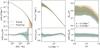 |
Fig. 4 Marginal halo mass function, power spectrum, and reduced bispectrum from the left to right panel for halo density fields with a virial mass between 3 × 10¹² h−1 M⊙ and 1 × 10¹³ h−1 M⊙ at a 7.81 h−1 Mpc voxel resolution. All curves were obtained from 30 catalogues, with the dashed green and the solid orange line representing the ensemble mean of PineTree mocks and validation data, respectively. The 1 σ line is outlined by the coloured shaded regions. The bottom subplot in each panel shows the ratio of the respective summary statistic between the mock and validation set where the shaded grey region is the 5% deviation threshold. |
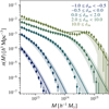 |
Fig. 5 Mean conditional halo mass functions predicted by the PineTree model in solid lines and the halo mass function estimated from N-body simulations depicted in diamonds. The different colours correspond to different underlying DM overdensity bins that are specified by the legend in the figure. Error bars correspond to the 1 σ deviation and are presented as solid vertical lines or as shaded regions for the N-body estimates and PineTree predictions, respectively. |
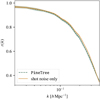 |
Fig. 6 Cross-correlation coefficient comparison for halos with masses between 3 × 10¹² h−1 M⊙ and 1 × 10¹³ h−1 M⊙ at a 7.81 h−1 Mpc voxel resolution from 30 validation samples. The dashed green line shows the mean for the cross-correlation coefficient from the mock fields, while the mean of idealised fields with only Poisson noise contributions is depicted in solid orange. The shaded coloured area shows the 1 σ region, respectively. |
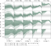 |
Fig. 7 Ratios between the power spectrum of the PineTree mocks and the validation catalogues for different mass bins and at voxel resolutions. For the subplots shown from left to right, the voxel size is decreasing according to the Table 1 and also indicated by the annotations in the top row. From top to bottom, each row shows the ratio for increasing mass bins. As with all previous figures, the quantities shown here were all computed using an ensemble of 30 fields. |
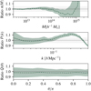 |
Fig. 8 Simplified version of Fig. 4 showing the ratios of the halo mass function, power spectrum, and reduced bispectrum but for input over-density fields from a 2LPT gravity model. The respective quantities were computed for halos with a virial mass between 3 × 10¹² h−1 M⊙ and 1 × 10¹³ h−1 M⊙ at a 7.81 h−1 Mpc voxel resolution. |
5.2 Approximate gravity model
The results in the previous subsection were predictions based on L-Gadget overdensity fields. In practice, we would like to substitute the input fields with overdensity fields from approximate gravity solvers to save even more computational time. Figure 8 shows the results from PineTree retrained using the density fields produced by a 2LPT model (as is described in Sect. 4.1). The figure is a simplified version of Fig. 4 and shows only the ratios for the halo mass function, the power spectrum, and the reduced bispectrum with respect to the reference halo catalogue. We can report that the precision of the prediction is almost identical to the set-up with the L-Gadget overdensity fields, showing that PineTree is able to interpolate correctly from the approximate DM fields to the high-resolution N-body halos.
5.3 Redshift dependency
The variation discussed in this subsection is the application of PineTree on L-Gadget DM overdensities and halo catalogues at a redshift of z = 1 (as is described in Sect. 4.1). We find that the retrained model performs very similar to the set-up at a red-shift of z = 0 with notably only a slightly worse agreement for the reduced bispectrum. Therefore, we derive that PineTree can potentially be used to generate halo mocks at different redshifts. Future studies of the model are planned to incorporate the redshift as a conditional parameter. The results for this set-up are shown in Fig. B.2.
5.4 Model interpretation
As was mentioned in Sect. 3, the architecture of the network is interpretable and the trained weights can yield insights into the optimisation task itself. In particular, we can draw intuition from the symmetric convolutional kernel on the effective environment size needed as an input for the network to predict the halo distribution for a given voxel.
The kernel as described in Sect. 3.1.1 is based on a multipole expansion and more specifically all set-ups use only the monopole. Figure 9 visualises a slice through each of the three kernels with varying sizes according to Table 1. All of the depicted kernels are from training runs in which the fields are gridded with a voxel size of 7.81 h−1 Mpc. We see that the absolute values of the kernel weights strongly decrease the further it is located from the centre of the kernel. Because the magnitude of each weight in a convolutional kernel indicates the relative importance of a given location of that patch, we can quantify the information content from an overdensity region needed to predict the subsequent halo properties. We report that the central kernel itself accounts for over 40% of the total kernel weight.
Since the loss function for PineTree is a likelihood, derived in Eq. (11), we can directly compare the set-ups with varying kernel sizes through the difference in log-likelihood computed on the validation set. Figure 10 depicts the comparison of the difference in the log-likelihood, Δ log ℒ, for four different kernel sizes with the 3 × 3 × 3 kernel as baseline. As was expected, the local kernel performs the worst and there is a strong improvement when adopting the baseline model that takes neighbouring voxels into account. Increasing the kernel size to 5 × 5 × 5 still yields a significant improvement in the log-likelihood, while adopting even larger kernels does not improve the mean difference in log-likelihood beyond the standard deviation computed on the validation samples. Figure 11 additionally visualises the performance across the N-point validation metrics. For the 9 × 9 × 9 kernel, we observe over-fitting that would need to be mitigated via more training data or the early-stopping technique often utilised in the machine learning community, but this would digress from the goal of this work. Therefore, we conclude that PineTree performs best in our resolution and parameterisation study for fields gridded at a voxel size of 7.81 h−1 Mpc and with a kernel size of 7 × 7 × 7.
Another notable finding lies within the central 3 × 3 patch of the kernel shown in Fig. 9. We can see that the signs between the central kernel weight and its adjacent weights are opposite to each other. Consequently, a given matter density voxel and its surrounding environment patch adjacent positive overdensity regions will lower the contribution to the feature vector, ψ. In contrast, voids with negative overdensity values will enhance the magnitude of the feature vector instead. Figure 12 shows that with increasing ψ the resulting conditional halo mass function shifts right towards high mass halos and also increases in amplitude. The result agrees with our physical intuition that extended overdensity regions yield less massive halos, while regions where the overdensity is accumulated into a more condensed region will give rise to the most massive halos in our universe (or simulation). Moreover, one can observe that the kernels in Fig. 9 appear to be axis-aligned rather than purely isotropic, which is due to the unphysical density estimation through the CIC kernel, showing that PineTree is able to adjust for the alignment artefacts even with its constraint kernel set-up. We show in Appendix B.3 that the kernel weights are distributed more isotropically when using the computationally more expensive smoothed-particle hydrodynamics (SPH) interpolation (first described by Lucy 1977; Gingold & Monaghan 1977).
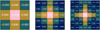 |
Fig. 9 Trained kernel weights from the central slice through the monopole kernel of PineTree. Each panel each from left to right shows a different kernel with sizes of 33, 53, and 73, respectively. The weights from the kernels are from optimisation runs at a 7.81 h−1 Mpc voxel resolution and the underlying colour indicates the absolute value of each weight. |
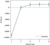 |
Fig. 10 Mean log-likelihood difference computed from the 30 validation simulations for PineTree with varying kernel sizes. The horizontal black line indicates the baseline model and represents the 3 × 3 × 3 kernel set-up. Error bars for each point indicate the 1 σ deviation obtained from the validation set. |
5.5 Computational cost
One of the key differences between our modelling approach and conventional machine-learning methods is the significantly reduced number of parameters. This leads to a model that is computationally efficient to train, both in terms of the required number of training samples and in computational time. We report as an example the number of training simulations needed to saturate the validation loss of PineTree for the 33 kernel set-up at a 7.81 h−1 Mpc voxel size resolution. The final mean validation log-likelihoods computed for the 30 validation samples after training for a given training sample size are listed in Table 2. Again, we have made use of the likelihood (see Eq. (11)) to assess the training run via the difference in log-likelihood with the baseline model using only one simulation for training. Already, the mean log-likelihood difference between one and five training simulations is significantly smaller than the standard deviation computed on the validation set and the difference becomes even more negligible when increasing the training set size. This shows that PineTree can generalise well with a small number of training samples, and we were very conservative in our choice to train all our optimisation runs with the ten aforementioned training simulations.
We conclude this section by reporting the computational time for training as well as running the model to produce halo catalogues to give an idea of the computational speed of our model. The specific hardware used in this work was a 64-core AMD EPYC 7702 machine with 1 TB of RAM (hereafter referred to as the CPU machine) and a Nvidia V100 with 32 GB of RAM (denoted later on as the GPU machine). The training was exclusively executed on the GPU machine, and the training time mainly depended on the resolution on which the model was trained, as is reported in Table 3, as it determined the total number of voxels for which the likelihood needs to be evaluated. For instance, at 3.91 h−1 Mpc voxel resolution, we needed to compute over the likelihood for 10 × 1283 voxels, as opposed to the 50 h−1 Mpc resolution run, where the training sample consisted only of 10 × 103 voxels. Due to the limited number of parameters, it would be possible to reduce the training time for high-resolution runs by only using sub-boxes of the training simulations, but we postpone a detailed study on optimising training time for PineTree for future work. Finally, we report the numbers for sampling halo catalogues using the trained model. The sampling for a 500 h−1 Mpc simulation gridded at a resolution of 1283 voxels took about 3.2 seconds for the CPU and 3.7 seconds on the GPU. This would result in an estimated cost of 100 GPU hours of training plus 63 000 CPU hours to produce 1000 realisations of 4h−1 Gpc sized mock halo simulations, which is over an order of magnitude faster than PINNOCHIO (1024000 CPU hours), EZmocks (822000 CPU hours), or PATCHY (822000 CPU hours) reported by Monaco (2016).
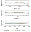 |
Fig. 11 Simplified version of Fig. 4 showing the halo mass function, power spectrum, and reduced bispectrum ratios but for different kernel sizes, as is specified in Table 1. The respective quantities were computed for halos with a virial mass between 3 × 10¹² h−1 M⊙ and 1 × 10¹³ h−1 M⊙ at a 7.81 h−1 Mpc voxel resolution. |
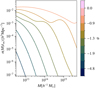 |
Fig. 12 Predicted conditional halo mass functions from PineTree for different values (indicated by the colour bar) of the feature map, ψ. The scalar is, as is described in Sect. 3.1.1, the output of the symmetric convolutional layer. |
Difference in log-likelihood depending on the number of training samples.
Training time in GPU hours for different gridding resolutions.
6 Conclusions
This paper has presented the computationally efficient neural network PineTree as a new approach to generating mock halo catalogues that are accurate on a percent level across various N-point correlation metrics. We built upon the work of Charnock et al. (2020), for which we further benchmarked and tested the limits of the model for a wide range of set-ups.
We performed an extensive resolution and parameter search to find that, in the current iteration, PineTree performs best at a voxel resolution of 7.81 h−1 Mpc and for halo masses between 3 × 10¹² h−1 M⊙ and 1 × 10¹³ h−1 M⊙. Here, we stress again that the metric utilised as the loss function during training is independent from the validation metrics; namely, the halo mass function, power spectrum, cross-correlation, and bispectrum. Therefore, this demonstrates the robustness of our model’s predictions. Similarly, the prediction accuracy translates well into set-ups with snapshots at a redshift of z = 1 and also for input density fields computed with a 2LPT algorithm. Notably, the use of PineTree in conjunction with approximate density fields makes it attractive as an emulator for future works to generate large mock simulation suites that can then be utilised; for instance, to compute numerical covariances.
Subsequently, we discussed how the physics-informed model architecture facilitates interpretability. The symmetric convolutional kernel and the simple network set-up enable insights into the effective environment size needed to predict the halo masses optimally on a given gridding resolution. In addition, the kernel reveals how the voxels in a density environment patch affect the resulting prediction and how much information each cell holds. Furthermore, the physical Poisson likelihood employed as a loss function allows the seamless integration of PineTree as the bias model into a galaxy clustering inference pipeline. A natural follow-up study will leverage this alongside the model’s reduced parameter space and differentiability within an inference with the algorithm BORG (Jasche & Wandelt 2013; Jasche et al. 2015; Lavaux & Jasche 2016; Jasche & Lavaux 2019; Lavaux et al. 2019).
Finally, we have shown in this work that PineTree is not only computationally efficient for sampling halo catalogues but also for training. This makes the pipeline easily adaptable to different model set-ups without the need for large training datasets.
We see that the model’s predictions start to break down for halo masses greater than 1 × 10¹⁴ h−1 M⊙ and high gridding resolutions, notably at 3.91 h−1 Mpc. The cause of this breakdown is related to the assumption of the underlying halo distribution. First, DM halos follow a Poisson distribution, and second, each voxel is independently distributed. Future iterations of PineTree can address these issues through the replacement of the loss and sampling procedure by a distribution-agnostic neural density estimator, as was done by Pandey et al. (2023), or by incorporating a more flexible likelihood such as the generalised Poisson distribution (Consul & Jain 1973). To account for the halo conditional distribution across neighbouring voxels, a mass conservation scheme or multi-scale approach could be explored.
There are numerous potential applications of PineTree to be tested. Future extensions to this work could be the prediction of other halo properties like velocities or the direct generation of mock galaxy catalogues. Another interesting aspect is the conditioning of PineTree on cosmological parameters.
Acknowledgements
We thank Metin Ata, Deaglan Bartlett, Nai Boonkongkird, Ludvig Doeser, Matthew Ho, Axel Lapel, Lucas Makinen, Stuart McAlpine, and Stephen Stopyra for useful discussions related to this work. We also thank Deaglan Bartlett, Ludvig Doeser, and Stuart McAlpine for their helpful feedback to improve the manuscript. This work has made use of the Infinity cluster hosted by Institut d’Astrophysique de Paris. We thank the efforts of S. Rouberol for running the cluster smoothly. This work was granted access to the HPC resources of Joliot Curie/TGCC (Très Grand Centre de Calcul) under the allocation AD010413589R1. This work was enabled by the research project grant ‘Understanding the Dynamic Universe’ funded by the Knut and Alice Wallenberg Foundation under Dnr KAW 2018.0067. JJ acknowledges support from the Swedish Research Council (VR) under the project 2020-05143 – ‘Deciphering the Dynamics of Cosmic Structure’. GL and SD acknowledge the grant GCEuclid from ‘Centre National d’Etudes Spatiales’ (CNES). This work was supported by the Simons Collaboration on ‘Learning the Universe’. This work is conducted within the Aquila Consortium (https://aquila-consortium.org).
Appendix A Simulation validation
As described in Sect. 4.1, we compare the matter power spectrum and halo mass function with theoretical predictions to validate the simulations we generated with L-Gadget and ROCKSTAR. Figure A.1 shows that the matter power spectra of the 60 simulations match the non-linear theoretical prediction computed by CLASS (as described in Audren & Lesgourgues 2011) very well for the Planck 2018 cosmological parameters (Planck Collaboration VI 2020). Similarly, the halo mass function reported by Tinker et al. (2008) is in good agreement with the halo mass functions from the final ROCKSTAR halo catalogues as shown in Fig. A.2. Therefore, we conclude that the simulation runs completed as expected and do not contain inherent errors that could bias our results in Sect. 5 obtained from the optimisations with PineTree.
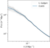 |
Fig. A.1 Matter power spectrum computed from by the Boltzmann solver CLASS with non-linear corrections at redshift z = 0 depicted by the solid blue line and the matter power spectra from the N-body simulations obtained from L-Gadget in light grey. Each grey line corresponds to one realisation from the simulation. |
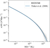 |
Fig. A.2 Halo mass function comparison between Tinker et al. (2008, in solid blue) and the N-body simulations (in light grey) produced by L-Gadget and ROCKSTAR as halo finder. The halo mass function is for halos adopting the virial mass definition (Bryan & Norman 1998) at redshift z = 0. Each grey line corresponds to one realisation from the simulation. |
Appendix B PineTree optimisation runs
B.1 Mixture component testing
Following the description of Sect. 4.2, we ran additional optimisations for different numbers of mixture components Nmix in PineTree namely two, three, and four. Since the loss function is derived from a proper probability density (see Sect. 3.2), we use the difference in the log-likelihood values computed on the validation simulations as the model comparison metric. Figure B.1 depicts the log-likelihood difference Δ log ℒ for the three different runs with respect to the baseline model with two mixture components as used throughout Sect. 5. We optimised the different model set-ups on snapshots at redshift z = 0 and field discretisation at a voxel resolution of 7.81 h−1 Mpc. We report that even though the models with more mixture components slightly improve the log-likelihood compared to the baseline model, the improvements are not significant as the mean difference in log-likelihood is still within the 1 σ standard deviation of the baseline. Hence, we limited our main resolution and parameter study to PineTree configurations with two mixture components.
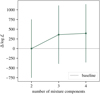 |
Fig. B.1 Mean difference in log-likelihood computed from the 30 validation simulations for different numbers of mixture components. The black horizontal line indicates the baseline model and represents the PineTree model with two mixture components. Error bars for each point indicate the 1 σ deviation obtained from the validation set. |
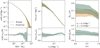 |
Fig. B.2 Same as Fig. 4 but with halos at z = 1. Again, the panels from left to right show the marginal halo mass distribution, the power spectrum and the reduced bispectrum with the network mocks plotted in green while the reference from the N-body simulations are shown in orange. The bottom subplot of each panel depicts the ratio of the respective summary statistics. The power spectrum and reduced bispectrum are computed using halos with a virial mass between 3 × 10¹² h−1 M⊙ and 1 × 10¹³ h−1 M⊙. |
B.2 Redshift z = 1 results
Following the results of Sect. 5.1, we optimise PineTree with snapshots at redshift z = 1 at a voxel resolution of 7.81 h−1 Mpc. Figure B.2 shows the same three key validation metrics after training. Comparing it to Fig. 4, the run at redshift z = 0, only the prediction for the reduced bispectrum is noticeably worse.
B.3 Density fields from smoothed-particle hydrodynamics
As pointed out in Sect. 5.4, the optimisation with the overdensity fields computed via CIC leads to kernels that show axis-aligned effects (see Fig. 9). To validate that this observed behaviour is not due to the model architecture itself, we retrain the same PineTree model as described in Sect. 5.1 at 7.81 h−1 Mpc voxel resolution, but with overdensity fields from L-Gadget estimated by the SPH algorithm. We applied the SPH implementation developed and used by Colombi et al. (2007). Since the SPH interpolation scheme preserves the isotropic properties of the underlying particle distribution better than the CIC approach, we expect the change in the mass assignment scheme to be reflected by the resulting convolutional kernel. Figure B.3 shows the trained kernel weights for the central slice. Comparing them to Fig. 9, we notice that the kernel weights appear more isotropic. Hence, we conclude that the axis-aligned weights as shown in Fig. 9 are caused by non-isotropic artefacts from the CIC interpolation.
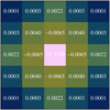 |
Fig. B.3 Central slice through a a 5 × 5 × 5 monopole kernel of PineTree (similar to Fig. 9). The weights are obtained through an optimisation run at 7.81 h−1 Mpc voxel resolution and DM overdensity fields computed using an SPH algorithm. The underlying colour indicates the absolute value of each weight. |
References
- Anagnostidis, S., Thomsen, A., Kacprzak, T., et al. 2022, arXiv e-prints [arXiv:2211.12346] [Google Scholar]
- Aubert, D., Pichon, C., & Colombi, S. 2004, MNRAS, 352, 376 [Google Scholar]
- Audren, B., & Lesgourgues, J. 2011, J. Cosmol. Astropart. Phys., 2011, 037 [CrossRef] [Google Scholar]
- Avila, S., Murray, S. G., Knebe, A., et al. 2015, MNRAS, 450, 1856 [NASA ADS] [CrossRef] [Google Scholar]
- Balaguera-Antolínez, A., Kitaura, F.-S., Pellejero-Ibáñez, M., Zhao, C., & Abel, T. 2018, MNRAS, 483, L58 [Google Scholar]
- Balaguera-Antolínez, A., Kitaura, F.-S., Pellejero-Ibáñez, M., et al. 2019, MNRAS, 491, 2565 [Google Scholar]
- Balaguera-Antolínez, A., Kitaura, F.-S., Alam, S., et al. 2023, A&A, 673, A130 [NASA ADS] [CrossRef] [EDP Sciences] [Google Scholar]
- Baldauf, T., Seljak, U. c. v., Smith, R. E., Hamaus, N., & Desjacques, V. 2013, Phys. Rev. D, 88, 083507 [NASA ADS] [CrossRef] [Google Scholar]
- Bardeen, J. M., Bond, J. R., Kaiser, N., & Szalay, A. S. 1986, ApJ, 304, 15 [Google Scholar]
- Bartlett, D. J., Ho, M., & Wandelt, B. D. 2024, ApJ, submitted [arXiv:2405.00635] [Google Scholar]
- Behroozi, P. S., Conroy, C., & Wechsler, R. H. 2010, ApJ, 717, 379 [Google Scholar]
- Behroozi, P. S., Wechsler, R. H., & Wu, H.-Y. 2013, ApJ, 762, 109 [NASA ADS] [CrossRef] [Google Scholar]
- Berger, P., & Stein, G. 2018, MNRAS, 482, 2861 [Google Scholar]
- Beyond-2pt Collaboration (Kause, E., et al.) 2024, arXiv e-prints [arXiv:2405.02252] [Google Scholar]
- Blas, D., Lesgourgues, J., & Tram, T. 2011, J. Cosmol. Astropart. Phys., 2011, 034 [CrossRef] [Google Scholar]
- Blot, L., Corasaniti, P. S., Amendola, L., & Kitching, T. D. 2016, MNRAS, 458, 4462 [NASA ADS] [CrossRef] [Google Scholar]
- Blot, L., Crocce, M., Sefusatti, E., et al. 2019, MNRAS, 485, 2806 [NASA ADS] [CrossRef] [Google Scholar]
- Bond, J. R. 1987, in Cosmology and Particle Physics, ed. I. Hinchliffe, 22 [Google Scholar]
- Bond, J. R., & Myers, S. T. 1996, ApJS, 103, 1 [NASA ADS] [CrossRef] [Google Scholar]
- Bond, J. R., Szalay, A. S., & Silk, J. 1988, ApJ, 324, 627 [NASA ADS] [CrossRef] [Google Scholar]
- Bond, J. R., Cole, S., Efstathiou, G., & Kaiser, N. 1991, ApJ, 379, 440 [NASA ADS] [CrossRef] [Google Scholar]
- Boonkongkird, C., Lavaux, G., Peirani, S., et al. 2023, arXiv e-prints [arXiv:2303.17939] [Google Scholar]
- Braun, R., Bonaldi, A., Bourke, T., Keane, E., & Wagg, J. 2019, arXiv e-prints [arXiv:1912.12699] [Google Scholar]
- Bryan, G. L., & Norman, M. L. 1998, ApJ, 495, 80 [NASA ADS] [CrossRef] [Google Scholar]
- Carlberg, R. G., & Couchman, H. M. P. 1989, ApJ, 340, 47 [NASA ADS] [CrossRef] [Google Scholar]
- Casas-Miranda, R., Mo, H. J., Sheth, R. K., & Boerner, G. 2002, MNRAS, 333, 730 [NASA ADS] [CrossRef] [Google Scholar]
- Cen, R., & Ostriker, J. P. 1993, ApJ, 417, 415 [NASA ADS] [CrossRef] [Google Scholar]
- Chan, K. C., Scoccimarro, R., & Sheth, R. K. 2012, Phys. Rev. D, 85, 083509 [CrossRef] [Google Scholar]
- Charnock, T., Lavaux, G., Wandelt, B. D., et al. 2020, MNRAS, 494, 50 [NASA ADS] [CrossRef] [Google Scholar]
- Chartier, N., & Wandelt, B. D. 2021, MNRAS, 509, 2220 [NASA ADS] [Google Scholar]
- Chartier, N., Wandelt, B., Akrami, Y., & Villaescusa-Navarro, F. 2021, MNRAS, 503, 1897 [NASA ADS] [CrossRef] [Google Scholar]
- Chaves-Montero, J., Angulo, R. E., Schaye, J., et al. 2016, MNRAS, 460, 3100 [NASA ADS] [CrossRef] [Google Scholar]
- Chuang, C.-H., Kitaura, F.-S., Prada, F., Zhao, C., & Yepes, G. 2014, MNRAS, 446, 2621 [Google Scholar]
- Chuang, C.-H., Zhao, C., Prada, F., et al. 2015, MNRAS, 452, 686 [CrossRef] [Google Scholar]
- Cole, S., & Kaiser, N. 1988, MNRAS, 233, 637 [NASA ADS] [Google Scholar]
- Cole, S., & Kaiser, N. 1989, MNRAS, 237, 1127 [NASA ADS] [Google Scholar]
- Colombi, S. 2013, AdaptaHOP: Subclump Finder, Astrophysics Source Code Library [record ascl:1305.004] [Google Scholar]
- Colombi, S., Chodorowski, M. J., & Teyssier, R. 2007, MNRAS, 375, 348 [NASA ADS] [CrossRef] [Google Scholar]
- Consul, P. C., & Jain, G. C. 1973, Technometrics, 15, 791 [CrossRef] [Google Scholar]
- Contarini, S., Pisani, A., Hamaus, N., et al. 2023, ApJ, 953, 46 [NASA ADS] [CrossRef] [Google Scholar]
- Davis, M., Efstathiou, G., Frenk, C. S., & White, S. D. M. 1985, ApJ, 292, 371 [Google Scholar]
- de la Torre, S., & Peacock, J. A. 2013, MNRAS, 435, 743 [CrossRef] [Google Scholar]
- de Santi, N. S. M., Shao, H., Villaescusa-Navarro, F., et al. 2023, ApJ, 952, 69 [NASA ADS] [CrossRef] [Google Scholar]
- Dekel, A., & Lahav, O. 1999, ApJ, 520, 24 [Google Scholar]
- DESI Collaboration (Aghamousa, A., et al.) 2016, arXiv e-prints [arXiv:1611.00036] [Google Scholar]
- Desjacques, V., Jeong, D., & Schmidt, F. 2018, Phys. Rep., 733, 1 [Google Scholar]
- Ding, J., Li, S., Zheng, Y., et al. 2024, ApJS, 270, 25 [NASA ADS] [CrossRef] [Google Scholar]
- Doeser, L., Jamieson, D., Stopyra, S., et al. 2023, arXiv e-prints [arXiv:2312.09271] [Google Scholar]
- Doré, O., Bock, J., Ashby, M., et al. 2014, arXiv e-prints [arXiv:1412.4872] [Google Scholar]
- Drinkwater, M. J., Jurek, R. J., Blake, C., et al. 2010, MNRAS, 401, 1429 [CrossRef] [Google Scholar]
- Efstathiou, G., & Rees, M. J. 1988, MNRAS, 230, 5 [Google Scholar]
- Efstathiou, G., Frenk, C. S., White, S. D. M., & Davis, M. 1988, MNRAS, 235, 715 [NASA ADS] [CrossRef] [Google Scholar]
- Eisenstein, D. J., & Hut, P. 1998, ApJ, 498, 137 [NASA ADS] [CrossRef] [Google Scholar]
- Euclid Collaboration (Castander, F. J., et al.) 2024a, A&A, submitted [Google Scholar]
- Euclid Collaboration (Mellier, Y., et al.) 2024b, A&A, in press, https://doi.org/10.1051/0004-6361/202450810 [Google Scholar]
- Feng, Y., Chu, M.-Y., Seljak, U., & McDonald, P. 2016, MNRAS, 463, 2273 [NASA ADS] [CrossRef] [Google Scholar]
- Ferrero, I., Crocce, M., Tutusaus, I., et al. 2021, A&A, 656, A106 [NASA ADS] [CrossRef] [EDP Sciences] [Google Scholar]
- Fisher, J. D., & Faltenbacher, A. 2017, MNRAS, 473, 3941 [Google Scholar]
- Fluri, J., Kacprzak, T., Lucchi, A., et al. 2019, Phys. Rev. D, 100, 063514 [Google Scholar]
- Fry, J. N., & Gaztanaga, E. 1993, ApJ, 413, 447 [NASA ADS] [CrossRef] [Google Scholar]
- García-Farieta, J. E., Balaguera-Antolínez, A., & Kitaura, F.-S. 2024, arXiv e-prints [arXiv:2405.10319] [Google Scholar]
- Garrison, L. H., Eisenstein, D. J., Ferrer, D., et al. 2018, ApJS, 236, 43 [NASA ADS] [CrossRef] [Google Scholar]
- Gingold, R. A., & Monaghan, J. J. 1977, MNRAS, 181, 375 [NASA ADS] [CrossRef] [Google Scholar]
- Green, J., Schechter, P., Baltay, C., et al. 2012, arXiv e-prints [arXiv:1208.4012] [Google Scholar]
- Hahn, C., Eickenberg, M., Ho, S., et al. 2023, PNAS, 120, e2218810120 [NASA ADS] [CrossRef] [Google Scholar]
- Hamaus, N., Seljak, U. c. v., Desjacques, V., Smith, R. E., & Baldauf, T. 2010, Phys. Rev. D, 82, 043515 [CrossRef] [Google Scholar]
- Hamaus, N., Pisani, A., Choi, J.-A., et al. 2020, J. Cosmology Astropart. Phys., 2020, 023 [CrossRef] [Google Scholar]
- Hermans, J., Delaunoy, A., Rozet, F., et al. 2021, arXiv e-prints [arXiv:2110.06581] [Google Scholar]
- Ho, M., Bartlett, D. J., Chartier, N., et al. 2024, Open J. Astrophys., accepted [arXiv:2402.05137] [Google Scholar]
- Hockney, R. W., & Eastwood, J. W. 1981, Computer Simulation Using Particles [Google Scholar]
- Hou, J., Dizgah, A. M., Hahn, C., et al. 2024, Phys. Rev. D, 109, 103528 [NASA ADS] [CrossRef] [Google Scholar]
- Howlett, C., Manera, M., & Percival, W. 2015a, Astron. Comput., 12, 109 [NASA ADS] [CrossRef] [Google Scholar]
- Howlett, C., Ross, A. J., Samushia, L., Percival, W. J., & Manera, M. 2015b, MNRAS, 449, 848 [NASA ADS] [CrossRef] [Google Scholar]
- Ishiyama, T., Prada, F., Klypin, A. A., et al. 2021, MNRAS, 506, 4210 [NASA ADS] [CrossRef] [Google Scholar]
- Izard, A., Crocce, M., & Fosalba, P. 2016, MNRAS, 459, 2327 [NASA ADS] [CrossRef] [Google Scholar]
- Jamieson, D., Li, Y., de Oliveira, R. A., et al. 2023, ApJ, 952, 145 [NASA ADS] [CrossRef] [Google Scholar]
- Jasche, J., & Wandelt, B. D. 2013, MNRAS, 432, 894 [Google Scholar]
- Jasche, J., & Lavaux, G. 2019, A&A, 625, A64 [NASA ADS] [CrossRef] [EDP Sciences] [Google Scholar]
- Jasche, J., Leclercq, F., & Wandelt, B. D. 2015, J. Cosmology Astropart. Phys., 2015, 036 [CrossRef] [Google Scholar]
- Jindal, V., Liang, A., Singh, A., Ho, S., & Jamieson, D. 2023, arXiv e-prints [arXiv:2303.13056] [Google Scholar]
- Jing, Y. P., Mo, H. J., & Börner, G. 1998, ApJ, 494, 1 [NASA ADS] [CrossRef] [Google Scholar]
- Kaiser, N. 1984, ApJ, 284, L9 [NASA ADS] [CrossRef] [Google Scholar]
- Kaiser, N. 1988, Symp. Int. Astron. Union, 130, 43 [NASA ADS] [CrossRef] [Google Scholar]
- Kazin, E. A., Koda, J., Blake, C., et al. 2014, MNRAS, 441, 3524 [NASA ADS] [CrossRef] [Google Scholar]
- Kingma, D. P., & Ba, J. 2014, arXiv e-prints [arXiv:1412.6980] [Google Scholar]
- Kitaura, F.-S., Yepes, G., & Prada, F. 2013, MNRAS, 439, L21 [Google Scholar]
- Kitaura, F.-S., Gil-Marín, H., Scóccola, C. G., et al. 2015, MNRAS, 450, 1836 [NASA ADS] [CrossRef] [Google Scholar]
- Kitaura, F.-S., Rodríguez-Torres, S., Chuang, C.-H., et al. 2016, MNRAS, 456, 4156 [NASA ADS] [CrossRef] [Google Scholar]
- Kitaura, F.-S., Balaguera-Antolínez, A., Sinigaglia, F., & Pellejero-Ibáñez, M. 2022, MNRAS, 512, 2245 [NASA ADS] [CrossRef] [Google Scholar]
- Knollmann, S. R., & Knebe, A. 2009, ApJS, 182, 608 [Google Scholar]
- Koda, J., Blake, C., Beutler, F., Kazin, E., & Marin, F. 2016, MNRAS, 459, 2118 [NASA ADS] [CrossRef] [Google Scholar]
- Kravtsov, A. V., & Klypin, A. A. 1999, ApJ, 520, 437 [NASA ADS] [CrossRef] [Google Scholar]
- Laureijs, R., Amiaux, J., Arduini, S., et al. 2011, arXiv e-prints [arXiv:1110.3193] [Google Scholar]
- Lavaux, G., & Jasche, J. 2016, MNRAS, 455, 3169 [Google Scholar]
- Lavaux, G., Jasche, J., & Leclercq, F. 2019, MNRAS, submitted [arXiv:1909.06396] [Google Scholar]
- Leclercq, F., Faure, B., Lavaux, G., et al. 2020, A&A, 639, A91 [NASA ADS] [CrossRef] [EDP Sciences] [Google Scholar]
- LeCun, Y., Boser, B., Denker, J. S., et al. 1989, Neural Computat., 1, 541 [CrossRef] [Google Scholar]
- Legin, R., Ho, M., Lemos, P., et al. 2024, MNRAS, 527, L173 [Google Scholar]
- Lehmann, B. V., Mao, Y.-Y., Becker, M. R., Skillman, S. W., & Wechsler, R. H. 2017, ApJ, 834, 37 [NASA ADS] [CrossRef] [Google Scholar]
- Lesgourgues, J. 2011, arXiv e-prints [arXiv:1104.2932] [Google Scholar]
- LSST Science Collaboration (Abell, P. A., et al.) 2009, arXiv e-prints [arXiv:0912.0201] [Google Scholar]
- Lucy, L. B. 1977, AJ, 82, 1013 [NASA ADS] [CrossRef] [Google Scholar]
- Makinen, T. L., Charnock, T., Lemos, P., et al. 2022, Open J. Astrophys., 5, 18 [NASA ADS] [CrossRef] [Google Scholar]
- Manera, M., Scoccimarro, R., Percival, W. J., et al. 2012, MNRAS, 428, 1036 [Google Scholar]
- Manera, M., Samushia, L., Tojeiro, R., et al. 2014, MNRAS, 447, 437 [Google Scholar]
- Matsubara, T. 1999, ApJ, 525, 543 [NASA ADS] [CrossRef] [Google Scholar]
- Merz, H., Pen, U.-L., & Trac, H. 2005, New Astron., 10, 393 [CrossRef] [Google Scholar]
- Mo, H. J., & White, S. D. M. 1996, MNRAS, 282, 347 [Google Scholar]
- Modi, C., Feng, Y., & Seljak, U. 2018, J. Cosmology Astropart. Phys., 2018, 028 [CrossRef] [Google Scholar]
- Monaco, P. 2016, Galaxies, 4, 53 [NASA ADS] [CrossRef] [Google Scholar]
- Monaco, P., Theuns, T., & Taffoni, G. 2002a, MNRAS, 331, 587 [Google Scholar]
- Monaco, P., Theuns, T., Taffoni, G., et al. 2002b, ApJ, 564, 8 [NASA ADS] [CrossRef] [Google Scholar]
- Moster, B. P., Somerville, R. S., Maulbetsch, C., et al. 2010, ApJ, 710, 903 [Google Scholar]
- Narayan, R., & White, S. D. M. 1988, MNRAS, 231, 97 [Google Scholar]
- Nelson, D., Springel, V., Pillepich, A., et al. 2019, CompAC, 6, 1 [Google Scholar]
- Neyrinck, M. C., Hamilton, A. J. S., & Gnedin, N. Y. 2005, MNRAS, 362, 337 [CrossRef] [Google Scholar]
- Neyrinck, M. C., Aragón-Calvo, M. A., Jeong, D., & Wang, X. 2014, MNRAS, 441, 646 [Google Scholar]
- Nguyen, N.-M., Schmidt, F., Lavaux, G., & Jasche, J. 2021, J. Cosmology Astropart. Phys., 2021, 058 [CrossRef] [Google Scholar]
- Nguyen, N.-M., Schmidt, F., Tucci, B., Reinecke, M., & Kostić, A. 2024, arXiv e-prints [arXiv:2403.03220] [Google Scholar]
- Nishimichi, T., Shirata, A., Taruya, A., et al. 2009, PASJ, 61, 321 [NASA ADS] [Google Scholar]
- Nishimichi, T., Taruya, A., Koyama, K., & Sabiu, C. 2010, J. Cosmology Astropart. Phys., 2010, 002 [CrossRef] [Google Scholar]
- Paillas, E., Cuesta-Lazaro, C., Zarrouk, P., et al. 2023, MNRAS, 522, 606 [CrossRef] [Google Scholar]
- Pandey, S., Modi, C., Wandelt, B. D., & Lavaux, G. 2023, in NeurIPS 2023 AI for Science Workshop [Google Scholar]
- Peacock, J. A., & Smith, R. E. 2000, MNRAS, 318, 1144. [Google Scholar]
- Pellejero Ibañez, M., Angulo, R. E., Jamieson, D., & Li, Y. 2024, MNRAS, 529, 89 [CrossRef] [Google Scholar]
- Pen, U.-L. 1998, ApJ, 504, 601 [NASA ADS] [CrossRef] [Google Scholar]
- Percival, W. J., Ross, A. J., Sánchez, A. G., et al. 2014, MNRAS, 439, 2531 [NASA ADS] [CrossRef] [Google Scholar]
- Perez, L. A., Genel, S., Villaescusa-Navarro, F., et al. 2023, ApJ, 954, 11 [NASA ADS] [CrossRef] [Google Scholar]
- Piras, D., Joachimi, B., & Villaescusa-Navarro, F. 2023, MNRAS, 520, 668 [Google Scholar]
- Planck Collaboration VI. 2020, A&A, 641, A6 [NASA ADS] [CrossRef] [EDP Sciences] [Google Scholar]
- Planelles, S., & Quilis, V. 2010, A&A, 519, A94 [NASA ADS] [CrossRef] [EDP Sciences] [Google Scholar]
- Porqueres, N., Heavens, A., Mortlock, D., Lavaux, G., & Makinen, T. L. 2023, arXiv e-prints [arXiv:2304.04785] [Google Scholar]
- Press, W. H., & Schechter, P. 1974, ApJ, 187, 425 [Google Scholar]
- Ravanbakhsh, S., Oliva, J., Fromenteau, S., et al. 2017, arXiv e-prints [arXiv:1711.02033] [Google Scholar]
- Reddick, R. M., Wechsler, R. H., Tinker, J. L., & Behroozi, P. S. 2013, ApJ, 771, 30 [Google Scholar]
- Régaldo-Saint Blancard, B., Hahn, C., Ho, S., et al. 2024, Phys. Rev. D, 109, 083535 [CrossRef] [Google Scholar]
- Repp, A., & Szapudi, I. 2020, MNRAS, 493, 3449 [NASA ADS] [CrossRef] [Google Scholar]
- Schaeffer, R., & Silk, J. 1985, ApJ, 292, 319 [NASA ADS] [CrossRef] [Google Scholar]
- Schaeffer, R., & Silk, J. 1988, ApJ, 332, 1 [NASA ADS] [CrossRef] [Google Scholar]
- Schmidt, F., Elsner, F., Jasche, J., Nguyen, N. M., & Lavaux, G. 2019, J. Cosmology Astropart. Phys., 2019, 042 [CrossRef] [Google Scholar]
- Scoccimarro, R., & Sheth, R. K. 2002, MNRAS, 329, 629 [NASA ADS] [CrossRef] [Google Scholar]
- Scott, D. W. 2015, Multivariate Density Estimation: Theory, Practice, and Visualization (John Wiley & Sons) [Google Scholar]
- Seljak, U. 2000, MNRAS, 318, 203 [Google Scholar]
- Seljak, U., & Warren, M. S. 2004, MNRAS, 355, 129 [CrossRef] [Google Scholar]
- Seljak, U., Aslanyan, G., Feng, Y., & Modi, C. 2017, J. Cosmology Astropart. Phys., 2017, 009 [CrossRef] [Google Scholar]
- Sheth, R. K., & Lemson, G. 1999, MNRAS, 304, 767 [CrossRef] [Google Scholar]
- Sheth, R. K., & Tormen, G. 1999, MNRAS, 308, 119 [Google Scholar]
- Sheth, R. K., & Tormen, G. 2002, MNRAS, 329, 61 [Google Scholar]
- Sheth, R. K., Mo, H. J., & Tormen, G. 2001, MNRAS, 323, 1 [NASA ADS] [CrossRef] [Google Scholar]
- Sheth, R. K., Chan, K. C., & Scoccimarro, R. 2013, Phys. Rev. D, 87, 083002 [NASA ADS] [CrossRef] [Google Scholar]
- Smith, R. E., Scoccimarro, R., & Sheth, R. K. 2007, Phys. Rev. D, 75, 063512 [NASA ADS] [CrossRef] [Google Scholar]
- Springel, V. 2005, MNRAS, 364, 1105 [Google Scholar]
- Springel, V., White, S. D. M., Tormen, G., & Kauffmann, G. 2001, MNRAS, 328, 726 [Google Scholar]
- Springel, V., Pakmor, R., Zier, O., & Reinecke, M. 2021, MNRAS, 506, 2871 [NASA ADS] [CrossRef] [Google Scholar]
- Stadel, J. G. 2001, Cosmological N-body Simulations and Their Analysis (University of Washington) [Google Scholar]
- Stiskalek, R., Desmond, H., Holvey, T., & Jones, M. G. 2021, MNRAS, 506, 3205 [NASA ADS] [CrossRef] [Google Scholar]
- Taffoni, G., Monaco, P., & Theuns, T. 2002, MNRAS, 333, 623 [NASA ADS] [CrossRef] [Google Scholar]
- Takada, M., Ellis, R. S., Chiba, M., et al. 2014, PASJ, 66, R1 [Google Scholar]
- Taruya, A., & Soda, J. 1999, ApJ, 522, 46 [NASA ADS] [CrossRef] [Google Scholar]
- Tassev, S., Zaldarriaga, M., & Eisenstein, D. J. 2013, J. Cosmology Astropart. Phys., 2013, 036 [CrossRef] [Google Scholar]
- Tassev, S., Eisenstein, D. J., Wandelt, B. D., & Zaldarriaga, M. 2015, arXiv e-prints [arXiv:1502.07751] [Google Scholar]
- Tegmark, M., & Bromley, B. C. 1999, ApJ, 518, L69 [Google Scholar]
- Teyssier, R. 2002, A&A, 385, 337 [CrossRef] [EDP Sciences] [Google Scholar]
- Tinker, J., Kravtsov, A. V., Klypin, A., et al. 2008, ApJ, 688, 709 [Google Scholar]
- Vakili, M., Kitaura, F.-S., Feng, Y., et al. 2017, MNRAS, 472, 4144 [CrossRef] [Google Scholar]
- Valageas, P., & Nishimichi, T. 2011, A&A, 527, A87 [NASA ADS] [CrossRef] [EDP Sciences] [Google Scholar]
- Vale, A., & Ostriker, J. P. 2004, MNRAS, 353, 189 [Google Scholar]
- Valogiannis, G., Yuan, S., & Dvorkin, C. 2024, Phys. Rev. D, 109, 103503 [NASA ADS] [CrossRef] [Google Scholar]
- van Uitert, Edo, Cacciato, Marcello, Hoekstra, Henk, & Herbonnet, Ricardo. 2015, A&A, 579, A26 [NASA ADS] [CrossRef] [EDP Sciences] [Google Scholar]
- Villaescusa-Navarro, F. 2018, Pylians: Python libraries for the analysis of numerical simulations, Astrophysics Source Code Library [record ascl:1811.008] [Google Scholar]
- Villaescusa-Navarro, F., Hahn, C., Massara, E., et al. 2020, ApJS, 250, 2 [CrossRef] [Google Scholar]
- Villaescusa-Navarro, F., Genel, S., Angles-Alcazar, D., et al. 2021, arXiv e-prints [arXiv:2109.10360] [Google Scholar]
- Villanueva-Domingo, P., & Villaescusa-Navarro, F. 2022, ApJ, 937, 115 [NASA ADS] [CrossRef] [Google Scholar]
- Wechsler, R. H., DeRose, J., Busha, M. T., et al. 2022, ApJ, 931, 145 [NASA ADS] [CrossRef] [Google Scholar]
- Weltman, A., Bull, P., Camera, S., et al. 2020, PASA, 37, e002 [Google Scholar]
- White, M., Tinker, J. L., & McBride, C. K. 2013, MNRAS, 437, 2594 [Google Scholar]
- Yang, X., Mo, H. J., & van den Bosch, F. C. 2003, MNRAS, 339, 1057 [Google Scholar]
- Yang, X., Mo, H. J., & van den Bosch, F. C. 2008, ApJ, 676, 248 [Google Scholar]
- Yang, X., Mo, H. J., & van den Bosch, F. C. 2009, ApJ, 695, 900 [Google Scholar]
- Yang, X., Zhang, Y., Lu, T., et al. 2017, ApJ, 848, 60 [NASA ADS] [CrossRef] [Google Scholar]
- Yuan, S., Abel, T., & Wechsler, R. H. 2023, MNRAS, 527, 1993 [NASA ADS] [CrossRef] [Google Scholar]
- Yung, L. Y. A., Somerville, R. S., Ferguson, H. C., et al. 2022a, MNRAS, 515, 5416 [NASA ADS] [CrossRef] [Google Scholar]
- Yung, L. Y. A., Somerville, R. S., Finkelstein, S. L., et al. 2022b, MNRAS, 519, 1578 [NASA ADS] [CrossRef] [Google Scholar]
- Zehavi, I., Zheng, Z., Weinberg, D. H., et al. 2011, ApJ, 736, 59 [NASA ADS] [CrossRef] [Google Scholar]
- Zhang, X., Wang, Y., Zhang, W., et al. 2019, arXiv e-prints [arXiv:1902.05965] [Google Scholar]
- Zheng, Z., Berlind, A. A., Weinberg, D. H., et al. 2005, ApJ, 633, 791 [NASA ADS] [CrossRef] [Google Scholar]
- Zhou, A. J., & Dodelson, S. 2023, Phys. Rev. D, 108, 083506 [NASA ADS] [CrossRef] [Google Scholar]
All Tables
All Figures
|
Fig. 1 Comparison between using one-point statistics (upper panel) and two-point statistics (lower panel) as validation metrics. The first panel on top shows a kernel density estimate plot of the number of voxels with a given halo count as a function of the underlying DM overdensity. Each line corresponds to the number of halos per voxel, as is indicated by the annotated text on the left. The distributions were produced using a Gaussian kernel with a bandwidth set according to Scott’s rule (Scott 2015). The dark blue, pink, and green curves show the number distribution obtained from N-body simulation, the TPL by Neyrinck et al. (2014), and PineTree respectively. In the bottom panel, we show the mean power spectrum from the generated fields and ratios with respect to the reference N-body simulation. The grey band indicates the 10% deviation threshold. |
| In the text | |
|
Fig. 2 Schematic view of the PineTree pipeline. The following steps are depicted from left to right: the input DM overdensity field was convolved with a rotation-symmetric kernel; a mixture density network computed the distribution parameters of a log-normal mixture distribution with the feature map, ψ halo masses were drawn from the emulated distributions to construct the final halo catalogue. |
| In the text | |
|
Fig. 3 Visualisation of a 5 × 5 × 5 monopole kernel. Identical colours indicate shared weights resulting in a rotationally symmetric pattern. |
| In the text | |
|
Fig. 4 Marginal halo mass function, power spectrum, and reduced bispectrum from the left to right panel for halo density fields with a virial mass between 3 × 10¹² h−1 M⊙ and 1 × 10¹³ h−1 M⊙ at a 7.81 h−1 Mpc voxel resolution. All curves were obtained from 30 catalogues, with the dashed green and the solid orange line representing the ensemble mean of PineTree mocks and validation data, respectively. The 1 σ line is outlined by the coloured shaded regions. The bottom subplot in each panel shows the ratio of the respective summary statistic between the mock and validation set where the shaded grey region is the 5% deviation threshold. |
| In the text | |
|
Fig. 5 Mean conditional halo mass functions predicted by the PineTree model in solid lines and the halo mass function estimated from N-body simulations depicted in diamonds. The different colours correspond to different underlying DM overdensity bins that are specified by the legend in the figure. Error bars correspond to the 1 σ deviation and are presented as solid vertical lines or as shaded regions for the N-body estimates and PineTree predictions, respectively. |
| In the text | |
|
Fig. 6 Cross-correlation coefficient comparison for halos with masses between 3 × 10¹² h−1 M⊙ and 1 × 10¹³ h−1 M⊙ at a 7.81 h−1 Mpc voxel resolution from 30 validation samples. The dashed green line shows the mean for the cross-correlation coefficient from the mock fields, while the mean of idealised fields with only Poisson noise contributions is depicted in solid orange. The shaded coloured area shows the 1 σ region, respectively. |
| In the text | |
|
Fig. 7 Ratios between the power spectrum of the PineTree mocks and the validation catalogues for different mass bins and at voxel resolutions. For the subplots shown from left to right, the voxel size is decreasing according to the Table 1 and also indicated by the annotations in the top row. From top to bottom, each row shows the ratio for increasing mass bins. As with all previous figures, the quantities shown here were all computed using an ensemble of 30 fields. |
| In the text | |
|
Fig. 8 Simplified version of Fig. 4 showing the ratios of the halo mass function, power spectrum, and reduced bispectrum but for input over-density fields from a 2LPT gravity model. The respective quantities were computed for halos with a virial mass between 3 × 10¹² h−1 M⊙ and 1 × 10¹³ h−1 M⊙ at a 7.81 h−1 Mpc voxel resolution. |
| In the text | |
|
Fig. 9 Trained kernel weights from the central slice through the monopole kernel of PineTree. Each panel each from left to right shows a different kernel with sizes of 33, 53, and 73, respectively. The weights from the kernels are from optimisation runs at a 7.81 h−1 Mpc voxel resolution and the underlying colour indicates the absolute value of each weight. |
| In the text | |
|
Fig. 10 Mean log-likelihood difference computed from the 30 validation simulations for PineTree with varying kernel sizes. The horizontal black line indicates the baseline model and represents the 3 × 3 × 3 kernel set-up. Error bars for each point indicate the 1 σ deviation obtained from the validation set. |
| In the text | |
|
Fig. 11 Simplified version of Fig. 4 showing the halo mass function, power spectrum, and reduced bispectrum ratios but for different kernel sizes, as is specified in Table 1. The respective quantities were computed for halos with a virial mass between 3 × 10¹² h−1 M⊙ and 1 × 10¹³ h−1 M⊙ at a 7.81 h−1 Mpc voxel resolution. |
| In the text | |
|
Fig. 12 Predicted conditional halo mass functions from PineTree for different values (indicated by the colour bar) of the feature map, ψ. The scalar is, as is described in Sect. 3.1.1, the output of the symmetric convolutional layer. |
| In the text | |
|
Fig. A.1 Matter power spectrum computed from by the Boltzmann solver CLASS with non-linear corrections at redshift z = 0 depicted by the solid blue line and the matter power spectra from the N-body simulations obtained from L-Gadget in light grey. Each grey line corresponds to one realisation from the simulation. |
| In the text | |
|
Fig. A.2 Halo mass function comparison between Tinker et al. (2008, in solid blue) and the N-body simulations (in light grey) produced by L-Gadget and ROCKSTAR as halo finder. The halo mass function is for halos adopting the virial mass definition (Bryan & Norman 1998) at redshift z = 0. Each grey line corresponds to one realisation from the simulation. |
| In the text | |
|
Fig. B.1 Mean difference in log-likelihood computed from the 30 validation simulations for different numbers of mixture components. The black horizontal line indicates the baseline model and represents the PineTree model with two mixture components. Error bars for each point indicate the 1 σ deviation obtained from the validation set. |
| In the text | |
|
Fig. B.2 Same as Fig. 4 but with halos at z = 1. Again, the panels from left to right show the marginal halo mass distribution, the power spectrum and the reduced bispectrum with the network mocks plotted in green while the reference from the N-body simulations are shown in orange. The bottom subplot of each panel depicts the ratio of the respective summary statistics. The power spectrum and reduced bispectrum are computed using halos with a virial mass between 3 × 10¹² h−1 M⊙ and 1 × 10¹³ h−1 M⊙. |
| In the text | |
|
Fig. B.3 Central slice through a a 5 × 5 × 5 monopole kernel of PineTree (similar to Fig. 9). The weights are obtained through an optimisation run at 7.81 h−1 Mpc voxel resolution and DM overdensity fields computed using an SPH algorithm. The underlying colour indicates the absolute value of each weight. |
| In the text | |
Current usage metrics show cumulative count of Article Views (full-text article views including HTML views, PDF and ePub downloads, according to the available data) and Abstracts Views on Vision4Press platform.
Data correspond to usage on the plateform after 2015. The current usage metrics is available 48-96 hours after online publication and is updated daily on week days.
Initial download of the metrics may take a while.