| Issue |
A&A
Volume 690, October 2024
|
|
|---|---|---|
| Article Number | A27 | |
| Number of page(s) | 15 | |
| Section | Cosmology (including clusters of galaxies) | |
| DOI | https://doi.org/10.1051/0004-6361/202450755 | |
| Published online | 27 September 2024 | |
Fast simulation mapping: From standard to modified gravity cosmologies using the bias assignment method
1
Instituto de Astrofísica de Canarias, s/n,
38205
La Laguna, Tenerife,
Spain
2
Departamento de Astrofísica, Universidad de La Laguna,
38206
La Laguna, Tenerife,
Spain
Received:
17
May
2024
Accepted:
4
August
2024
Abstract
Context. We assess the effectiveness of a non-parametric bias model in generating mock halo catalogues for modified gravity (MG) cosmologies, relying on the distribution of dark matter from either MG or Λ cold dark matter (ΛCDM) simulations.
Aims. We aim to generate halo catalogues that effectively capture the distinct impact of MG, ensuring high accuracy in both two- and three-point statistics for a comprehensive analysis of large-scale structures. We investigated the inclusion of MG in non-local bias to directly map the tracers onto ΛCDM fields, which would significantly reduce computational costs.
Methods. We employed the bias assignment method (BAM) to model halo distribution statistics by leveraging seven high-resolution COLA simulations of MG cosmologies. Taking cosmic-web dependences into account when learning the bias relations, we designed two experiments to map the MG effects: one utilising the consistent MG density fields and the other employing the benchmark ΛCDM density field.
Results. BAM generates MG halo catalogues from both calibration experiments with excellent summary statistics, achieving a ~1% accuracy in the power spectrum across a wide range of k modes, with minimal differences well below 10% for modes subject to cosmic variance, particularly below k < 0.07 h Mpc−1. The reduced bispectrum remains consistent with the reference catalogues within 10% for the studied configuration. Our results demonstrate that a non-linear and non-local bias description can model the effects of MG starting from a ΛCDM field.
Key words: cosmology: miscellaneous / dark energy / large-scale structure of Universe
Corresponding author; This email address is being protected from spambots. You need JavaScript enabled to view it.
© The Authors 2024
 Open Access article, published by EDP Sciences, under the terms of the Creative Commons Attribution License (https://creativecommons.org/licenses/by/4.0), which permits unrestricted use, distribution, and reproduction in any medium, provided the original work is properly cited.
This article is published in open access under the Subscribe to Open model. This email address is being protected from spambots. You need JavaScript enabled to view it. to support open access publication.
1 Introduction
Modified gravity (MG) theories serve as a straightforward (and the most used) alternative framework to the standard cosmo-logical model Λ cold dark matter ΛCDM), providing a means to address one of its key unknowns – the late-time accelerated expansion of the Universe (Sotiriou & Faraoni 2010; Capozziello & de Laurentis 2011; Joyce et al. 2016). To accurately explore the matter distribution on both small and large scales, reliable N-body simulations are indispensable, which, due to the incorporation of additional degrees of freedom to account for unique effects, pose more computational challenges compared to those employed for the ΛCDM model (Winther et al. 2015). Comprehensive testing of cosmological probes to assess the potential deviations of gravity from that predicted by general relativity (GR) demands the construction of accurate MG catalogues. This is particularly essential for meeting the precision and accuracy requirements expected by current galaxy surveys, including the Dark Energy Spectroscopic Instrument (DESI; DESI Collaboration 2016) survey and the Euclid mission (Laureijs et al. 2011). A variety of methods have been proposed in the literature to expedite the prediction of key observables in MG models and circumvent the high computing expense of full N-body simulations. Notable approaches involve the parametrisation of fitting functions tailored to accurately reproduce the matter power spectrum (Winther et al. 2019), the construction of emulators for efficient approximations (Ramachandra et al. 2021; Ruan et al. 2024; Brando et al. 2022; Arnold et al. 2022), and approaches based on the cosmology scaling technique introduced by Angulo & White (2010). These techniques have demonstrated the feasibility of casting some of the features of standard cosmology into their counterparts in MG models without the need of comprehensive N-body simulations for the latter (see e.g. Mead et al. 2015). While emulators and fitting functions excel in accurately capturing individual observables of the MG catalogues (e.g. the mass function, power spectrum, mass-density relations, etc.), these techniques lack the ability to provide an overall view of the summary statistics of the tracer distribution. For example, recent analyses suggest fitting functions based on the ratio of the power spectrum of MG to ΛCDM models, using N-body simulations along with HALOFIT (Smith et al. 2003). This approach separately reproduces the MG halo mass function for halos with masses above 8.2 × 10¹² h−1 M⊙ (see e.g. Gupta et al. 2022) and the non-linear power spectrum of MG up to non-linear scales of 3 h Mpc−1 with 5% accuracy (see e.g. Gupta et al. 2023). On a different front, the scaling technique has the ability to generate mock data for full halo catalogues, incorporating realistic non-linear effects into cosmological models with known background parameters. Specifically, when applied to MG simulations, this technique has shown to be efficient in reproducing MG catalogues with variations of up to ~3% in the matter power spectrum and up to ~5% in the halo mass function for scales up to k = 0.1 h Mpc−1 in Fourier space (Mead et al. 2015). Although this technique provides valuable insights that allow realistic non-linear effects to be simulated in alternative cosmologies, it faces limitations in accurately capturing the screening mechanisms and is unable to account for environment dependences, which is critical for MG models. The overall accuracy of the method will decrease as we scale for cosmologies that are farther away in cosmological parameter space from the original cosmology (see e.g. Contreras et al. 2020).
Alternative approaches have become increasingly important since detailed N-body simulations, which are run to obtain a complete description of the density field in MG scenarios, are computationally costly. In light of this, we propose a novel strategy that bypasses the computational demands of direct simulations by relying on the mock construction technique to make use of a smooth large-scale dark matter (DM) field obtained from given initial conditions, and populating it with halos (or galaxies) following a bias prescription. Several methods for speeding up the construction of mock catalogues while enhancing precision in their clustering statistics have been suggested in the literature, including PEAK PATCH (Bond & Myers 1996), PINOCCHIO (Monaco et al. 2002), PTHALOS (Scoccimarro & Sheth 2002), ICE-COLA (Tassev et al. 2013; Izard et al. 2016), PATCHY (Kitaura et al. 2014), QPM (White et al. 2014), EZmocks (Chuang et al. 2015), and HALOGEN (Avila et al. 2015), among others (see e.g. Berlind et al. 2003; Angulo et al. 2014; Manera et al. 2013, 2015; Carretero et al. 2015; Koda et al. 2016; Feng et al. 2016). Recently, two distinct approaches have been introduced and successfully validated: the non-parametric bias assignment method (BAM; Balaguera-Antolínez et al. 2019, 2023; Pellejero-Ibañez et al. 2020) and the parametric WebON method (further details are provided in Kitaura et al. 2024; Coloma-Nadal et al. 2024, and Kitaura et al. in prep). Throughout this paper, we mainly focus on the non-parametric method to perform the analysis of the MG density fields.
The BAM approach has demonstrated remarkable precision up to ~1% in the power spectrum at small scales (k ~ 1 h Mpc−1) and ~3–6% for typical configurations of the bispectrum when non-local information is included in the mock generation. A comparison of parametric (including second-order non-local bias) and non-parametric bias mapping techniques that use low-mass halos from ΛCDM simulations (of the order of ~108 h−1 M⊙) has been conducted by Pellejero-Ibañez et al. (2020). Their key finding suggests that non-parametric approaches such as BAM have the ability to replicate the three-point statistics of a halo distribution at low mass scales, where non-linear clustering and nonlocal dependences are likely to dominate. Recently, parametric bias models (Coloma-Nadal et al. 2024) have achieved a particularly high accuracy by including third-order non-local bias.
The goal of this paper is to assess whether a bias mapping method such as BAM is capable of reproducing the main features of halos from MG cosmologies given a smooth DM field of a ΛCDM cosmology. We present an alternative approach addressing the problem of generating fast and accurate MG catalogues while dealing with the limitations pointed out in previous studies. This methodology leverages the stochastic and scale-dependent bias description (Kitaura et al. 2014, 2015, 2016, 2021, 2022; Balaguera-Antolínez et al. 2020, 2023) to effectively map MG models based on a benchmark high-resolution ΛCDM simulation. The main assumption behind this approach is that the gravitational potential of the MG models can be expressed in terms of the conventional gravitational potential of GR under the correct bias transformation and, therefore, that it can produce the adequate cosmic tracer distribution for alternative cosmologies. With these two features together, we extend the mapping technique to encompass all scales while ensuring compatibility with summary statistics. This broadens the applicability of our method and enhances its accuracy across a wide range of scales. Additionally, we make use of a non-local bias description of the density fields, which captures additional intricate effects and provides a more comprehensive representation of the underlying density fields while extracting non-linear and non-local information from a reference simulation.
To reach this goal, we employed a set of high-resolution simulations of MG generated using the COLA (COmoving Lagrangian Acceleration) method. The COLA algorithm has been shown to perform well enough to produce mock catalogues for baryon acoustic oscillation (BAO) analysis (Ferrero et al. 2021). Recently, the COLA method was also used to perform cosmic shear analysis of simulated data from the Legacy Survey of Space and Time (LSST) Year 1, serving as a source for emulators; it exhibited remarkable fidelity, meeting stringent goodness-of-fit and parameter bias criteria across the prior and offering a promising avenue for extended cosmologies (see Gordon et al. 2024, for further details). This is of particular importance as MG models are prone to show distinctive patterns in the clustering of biased tracers that deviate from ΛCDM. These deviations emerge primarily on small scales in low cosmic density environments, where modifications of gravity strongly affect the growth of density perturbations and the overall matter distribution. Nevertheless, subtle large-scale effects may also become apparent given the impact of the smooth variation in the scale-dependent growth factor, cosmic environment, and tracer selection effects (see Jennings et al. 2012; He et al. 2013; Arnalte-Mur et al. 2017; Hernández-Aguayo et al. 2018; García-Farieta et al. 2021, and references therein).
The road map of this study is as follows. We ran a set of simulations of f(R) models that follow the Hu-Sawicki (HS) parametrisation (Hu & Sawicki 2007), which is one of the most studied MG models nowadays. The growth of density perturbations in f(R) gravity models is discussed in detail in Sect. 2. The simulations encompass six distinct scenarios, each characterised by a different level of deviation with respect to ΛCDM. They were specially designed to include configurations inside and outside of the confidence regions constrained by observations. Therefore, we considered cosmologies that mimic the clustering of ΛCDM and remain consistent with it, as well as cosmologies that deviate most from it and have already been ruled out by observations. The latter case is of interest because it allows us to evaluate the performance of BAM in capturing the MG signatures when considering models that significantly diverge from ΛCDM predictions. The DM field of the MG simulations, where each particle has a mass of Mp ≈ 1010 h−1 M⊙, serves as training data for BAM. Similarly, the reference catalogues correspond to the distribution of massive halos, each with at least 80 DM particles, obtained from a friends-of-friends (FoF) algorithm. The MG simulations and training dataset are described in detail in Sect. 3. Since our aim is to map ΛCDM into a MG model, we explored two analyses: one using the underlying DM field of a ΛCDM cosmology to perform the bias and kernel calibration with BAM in order to reproduce the reference MG halo number counts; and second, a calibration carried out with the MG DM field of each model to consistently reproduce their reference halo number counts. The methodology, including a brief description of the core of the BAM algorithm, is presented in detail in Sect. 4.1, as are the results and analysis of the aforementioned scenarios. Finally, we end with a summary and discussion in Sect. 5.
2 Dynamics in f(R) gravity models
Scalar-tensor theories are among the potential revisions to Einstein’s theory of gravity that have received the most attention (for an updated review, see e.g. Kobayashi 2019). Within the plethora of such theories, the f(R) gravity models constitute one of the most studied limits that add an extra degree of freedom to GR, where the gravitational action contains, apart from the metric, a scalar field that describes part of the gravitational field. In this subset of models, the Einstein-Hilbert action is modified by replacing the Ricci scalar, R, with a function of other curvature invariants such that R ↦ R + f(R). Of the various functional forms of f(R) that have been proposed in the literature (for a review, see e.g. Sotiriou & Faraoni 2010; De Felice & Tsujikawa 2010), we considered the HS template (Hu & Sawicki 2007), which provides a function that is able to satisfy the Solar System constraints as well as encode enough freedom to allow cosmic acceleration and structure formation to agree on large scales. The explicit form of HS f(R) function is
![Mathematical equation: $\[f(R)=-m^2 \frac{c_1\left(\frac{R}{m^2}\right)^n}{c_2\left(\frac{R}{m^2}\right)^n+1},\]$](/articles/aa/full_html/2024/10/aa50755-24/aa50755-24-eq1.png) (1)
(1)
where n, c1, and c2 are positive dimensionless parameters and ![Mathematical equation: $\[m^2 \equiv 8 \pi G \bar{\rho}_{c, 0} / 3=H_0^2 \Omega_m\]$](/articles/aa/full_html/2024/10/aa50755-24/aa50755-24-eq2.png) is a mass scale introduced in the model. The new dynamical degree of freedom is therefore represented by the scalar field (commonly called the ‘scalaron’), fR ≡ df(R)/dR, which can be approximated as
is a mass scale introduced in the model. The new dynamical degree of freedom is therefore represented by the scalar field (commonly called the ‘scalaron’), fR ≡ df(R)/dR, which can be approximated as
![Mathematical equation: $\[f_R \approx-n \frac{c_1}{c_2^2}\left(\frac{m^2}{R}\right)^{n+1}=\left(\frac{\Omega_m+4 \Omega_{\Lambda}}{\Omega_m a^{-3}+4 \Omega_{\Lambda}}\right)^{n+1} f_{R 0},\]$](/articles/aa/full_html/2024/10/aa50755-24/aa50755-24-eq3.png) (2)
(2)
with fR0 being the dimensionless scalar field at the present time. The rightmost expression of Eq. (2) was tuned to mimic to first order the background expansion of the ΛCDM model by setting c1/c2 = 6ΩΛ/Ωm. Moreover, the background curvature is given by R = 6(2H2 + H), so the bound condition f(R) → −2Λ is satisfied as a consequence of requiring equivalence with ΛCDM when |fR0| → 0. If the exponent n is assigned a specific value, then the model is fully specified by only one free parameter, fR0. In the simulations conducted for this paper, we explored two values of the exponent n: the first is n = 1, where we systematically varied |fR0| as 10−4, 10−5, and 10−6, denoted as F41, F51, and F61, respectively. The second value is n = 2, where we varied |fR0| as 10−3.5, 10−5, and 10−6.5, denoted as F3.52, F52, and F6.52. These choices were made to assess the robustness of our technique and to comprehensively cover current observational constraints.
Current constraints on HS models set the upper limit on the scalaron field at present time to |fR0| ⩽ 5.68 × 10⁻⁷ at 2σ confidence levels when using cluster abundances and galaxy clustering (Liu et al. 2021) and to |fR0| ⩽ × 10−6.75 when combining cosmic microwave background (CMB), BAO, and type Ia supernova (SNIa) with cosmic chronometers and redshift-space distortions (Wang 2021). Previous analyses were significantly relaxed, constraining |fR0| < 10−4.79 (Cataneo et al. 2015), < 5 × 10⁻⁶ (Shirasaki et al. 2016), and <3.7 × 10⁻⁶ at the 2σ confidence level (Boubekeur et al. 2014). Gravitational wave detection has also provided strong bounds, |fR0| < 5 × 10⁻⁷ at 1σ confidence (Vainio & Vilja 2017) and the so-called galaxy clustering ratio |fR0| < 5 × 10⁻⁶ at 68% confidence (Bel et al. 2015). This is competitive with astrophysical tests (Jain et al. 2013) and dwarf galaxies analysis (Vikram et al. 2013), which provide tighter constraints: |fR0| ≤ 5 × 10⁻⁷. The latest bounds using Subaru Hyper Suprime-Cam year 1 data are in agreement with ![Mathematical equation: $\[\log ~f_{R 0}=-6.38_{-1.41}^{+0.94}\]$](/articles/aa/full_html/2024/10/aa50755-24/aa50755-24-eq4.png) and
and ![Mathematical equation: $\[n=1.8_{-1.5}^{+1.1}\]$](/articles/aa/full_html/2024/10/aa50755-24/aa50755-24-eq5.png) , representing a substantial improvement in the constraints (Vazsonyi et al. 2021). Euclid’s future observations are expected to constrain log |fR0| at the 1% level using the full combination of spectroscopic and photometric galaxy clustering (Casas et al. 2023). Figure 1 depicts the constraints on the HS model in the log |fR0| − n plane. The orange confidence regions are reproduced from Cataneo et al. (2015) and correspond to the 68.3 and 95.4% confidence levels from the combination of clusters, CMB (Planck + WMAP + lensing + ACT and SPT) and SNIa + BAO. The blue confidence regions are reproduced from Vazsonyi et al. (2021) from cosmic shear analysis using Subaru Hyper Suprime-Cam year 1 data (Hikage et al. 2019). The coloured squares in Fig. 1 correspond to the location of the MG simulations in the log |fR0| − n plane relative to the actual constraints of these parameters. Therefore, our simulations span from models that faithfully reproduce nearly all features of the standard model to those that are ruled out by astrophysical probes.
, representing a substantial improvement in the constraints (Vazsonyi et al. 2021). Euclid’s future observations are expected to constrain log |fR0| at the 1% level using the full combination of spectroscopic and photometric galaxy clustering (Casas et al. 2023). Figure 1 depicts the constraints on the HS model in the log |fR0| − n plane. The orange confidence regions are reproduced from Cataneo et al. (2015) and correspond to the 68.3 and 95.4% confidence levels from the combination of clusters, CMB (Planck + WMAP + lensing + ACT and SPT) and SNIa + BAO. The blue confidence regions are reproduced from Vazsonyi et al. (2021) from cosmic shear analysis using Subaru Hyper Suprime-Cam year 1 data (Hikage et al. 2019). The coloured squares in Fig. 1 correspond to the location of the MG simulations in the log |fR0| − n plane relative to the actual constraints of these parameters. Therefore, our simulations span from models that faithfully reproduce nearly all features of the standard model to those that are ruled out by astrophysical probes.
An interesting feature of the HS model is that evades stringent constraints of deviations of GR on the Solar System scale by means of the chameleon mechanism (Khoury & Weltman 2004b,a; Mota & Shaw 2007). This mechanism leads to a complex interplay between the matter distribution and the magnitude of the fifth force that hides (or screens) any modification of gravity in some regions and separations. In fact, the scalar field’s action generates intriguing effects across all scales, with its influence effectively concealed in local environments (Winther et al. 2012; Llinares & Mota 2014; Ivarsen et al. 2016). According to local gravity constraints, the fifth force is extremely weak. However, high-density environments may conceal the fifth force via the chameleon mechanism. This is attributed to the inherent environmental dependence induced by the properties of DM distributions in the chameleon mechanism, which operates in such a way that the scalar field acquires a substantial mass in denser environments, rendering the fifth force negligible. Conversely, on cosmological scales, the scalar field remains light, resulting in significant modifications to gravity (Khoury & Weltman 2004b,a; Will 2014). A detailed discussion of the summary statistics in the HS model, based on simulations of matter, halos, and galaxies, can be found in Winther et al. (2015), Arnold & Li (2019), and Alam et al. (2021). Comparisons and modelling of clustering statistics in real- and redshift-space are presented in García-Farieta et al. (2019), Hernández-Aguayo et al. (2019), Wright et al. (2019), and García-Farieta et al. (2021).
The structure formation driven by the HS f(R) scalar field tends to amplify the growth of structure, leading to higher-density peaks compared to ΛCDM. On large scales, the clustering agrees with linear predictions, while on small scales, deviations from ΛCDM become larger due to the enhancement of gravity (for a detailed discussion on the non-linear structure formation in f(R) gravity models, see Oyaizu et al. 2008; Li et al. 2012b, 2013). This enhancement on small scales also results in an increased abundance of rare massive halos, which can substantially differ from the ΛCDM scenario depending on the magnitude of the background scalar field, fR0 (refer to Schmidt et al. 2009a, for halo statistics in f(R) models). In the linear regime, the perturbations are described by the modified Poisson equation (in Fourier space) for the gravitational potential, Φ, as k2Φ = −4πGeffa2δρ, with δρ being the fluctuation around the mean density and Geff the effective Newton’s constant that takes the form (Tsujikawa et al. 2008; Esposito-Farèse & Polarski 2001)
![Mathematical equation: $\[\frac{G_{\mathrm{eff}}}{G_{\mathrm{N}}}=\left\{\begin{array}{lr}1 & \mathrm{GR} \\1+k^2 /\left[3\left(k^2+a^2 m_{f_R}^2\right)\right] & f(R).\end{array}\right.\]$](/articles/aa/full_html/2024/10/aa50755-24/aa50755-24-eq6.png) (3)
(3)
Here, mfR is the mass of the scalar fluctuations (not to be confused with the mass scale, m, of the HS model). This quantity plays a crucial role in the chameleon mechanism as it establishes when the scalar field is suppressed. The linear growth for the matter fluctuations in these models is governed by (Lombriser 2014)
![Mathematical equation: $\[D^{\prime \prime}+\left[2-\frac{3}{2} \Omega_{\mathrm{m}}(a)\right] D^{\prime}-\frac{3}{2} \frac{G_{\mathrm{eff}}}{G_N} \Omega_{\mathrm{m}}(a) D \approx 0,\]$](/articles/aa/full_html/2024/10/aa50755-24/aa50755-24-eq7.png) (4)
(4)
where D = D(a, k) is the linear growth function and the derivatives are with respect to ln a. Note that both Geff and D are functions of time and scale, unlike the GR case in which both are independent of the scale. Figures 2 and 3 display the numerical solution of the effective gravitational constant and the linear growth factor as a function of time and scale (Eqs. (3) and (4), respectively). The different panels of the figures refer to the different HS models considered in this study, as indicated by their labels. The dashed grey line at z = 0.5 ![Mathematical equation: $\[(a=0 . \overline{6})\]$](/articles/aa/full_html/2024/10/aa50755-24/aa50755-24-eq8.png) represents the redshift of the simulation snapshots used for our analysis. Geff varies with the inverse square of the time and scale, as shown by the contours of Fig. 2. The area above the contour defined by Geff (k, a) = 1 shrinks with the scalar field strength, fR0, capturing deviations ranging from 5% up to 33% in the most extreme case (model F3.52). The intensity of the normalised Geff decreases as fR0 approaches zero, which is the ΛCDM scenario. This trend is clearly followed by the models F51, F61, and F6.52. Similarly, in Fig. 3 we observe the variation in D(a, k) across different scales and times. The disparity in the growth factor can reach up to 30% for the plotted time interval and scales (i.e. k ∈ [10−2, 1] h Mpc−1 and a ∈ [0.2, 1]). The most significant deviations from the ΛCDM growth factor can be seen at high Fourier modes, k ~ 1 h Mpc−1 (i.e. the middle non-linear regime of the structure formation), and at low redshifts. For models with larger |fR0|, such as |fR0| = 10−4, the chameleon screening is inefficient, as illustrated by the significant discrepancies in D of F41 compared to ΛCDM. Figure 4 shows the dynamics of Geff and D for the redshift of interest, z = 0.5; this essentially represents the cross-section of the contour plots depicted in Figs. 2 and 3 at the given redshift. Here, we clearly discern the deviations of each HS model from ΛCDM. At this redshift, Geff exhibits deviations of up to 33% for the most extreme model, F41 (red line), and deviations of up to 20% for the closest model to ΛCDM, F6.52 (cyan line). Intermediate deviations are observed for the remaining HS models, as depicted in the figure. Conversely, the growth factor follows a monotonic trend with respect to the scale and |fR0|, with deviations reaching 40% for F41 and remaining below 3% for f6.52. However, at small wavenumbers, D becomes increasingly indistinguishable from ΛCDM, especially for models with the lowest |fr0|. In contrast, Geff can still be distinguished from ΛCDM up to 7% at these scales for models with high |fR0|.
represents the redshift of the simulation snapshots used for our analysis. Geff varies with the inverse square of the time and scale, as shown by the contours of Fig. 2. The area above the contour defined by Geff (k, a) = 1 shrinks with the scalar field strength, fR0, capturing deviations ranging from 5% up to 33% in the most extreme case (model F3.52). The intensity of the normalised Geff decreases as fR0 approaches zero, which is the ΛCDM scenario. This trend is clearly followed by the models F51, F61, and F6.52. Similarly, in Fig. 3 we observe the variation in D(a, k) across different scales and times. The disparity in the growth factor can reach up to 30% for the plotted time interval and scales (i.e. k ∈ [10−2, 1] h Mpc−1 and a ∈ [0.2, 1]). The most significant deviations from the ΛCDM growth factor can be seen at high Fourier modes, k ~ 1 h Mpc−1 (i.e. the middle non-linear regime of the structure formation), and at low redshifts. For models with larger |fR0|, such as |fR0| = 10−4, the chameleon screening is inefficient, as illustrated by the significant discrepancies in D of F41 compared to ΛCDM. Figure 4 shows the dynamics of Geff and D for the redshift of interest, z = 0.5; this essentially represents the cross-section of the contour plots depicted in Figs. 2 and 3 at the given redshift. Here, we clearly discern the deviations of each HS model from ΛCDM. At this redshift, Geff exhibits deviations of up to 33% for the most extreme model, F41 (red line), and deviations of up to 20% for the closest model to ΛCDM, F6.52 (cyan line). Intermediate deviations are observed for the remaining HS models, as depicted in the figure. Conversely, the growth factor follows a monotonic trend with respect to the scale and |fR0|, with deviations reaching 40% for F41 and remaining below 3% for f6.52. However, at small wavenumbers, D becomes increasingly indistinguishable from ΛCDM, especially for models with the lowest |fr0|. In contrast, Geff can still be distinguished from ΛCDM up to 7% at these scales for models with high |fR0|.
Overall, the enhancement in the growth factor can be attributed to the effective mass of the scalar field, which limits the range of interaction of the fifth force, leaving, as a consequence, the growth on larger scales almost unaffected. In terms of distances, the effective length at which modifications of the gravitational potential take effect is given by the Compton wavelength of the scalaron field, which can be expressed in terms of fR0, given by
![Mathematical equation: $\[\lambda_C \equiv \frac{1}{m_{f_R}} \approx \frac{2997.92}{a} \sqrt{\frac{(n+1)\left|f_{R O}\right|\left(4-3 \Omega_m\right)^{n+1}}{\left[\Omega_m\left(a^{-3}-4\right)+4\right]^{n+2}}} h^{-1} \mathrm{Mpc}.\]$](/articles/aa/full_html/2024/10/aa50755-24/aa50755-24-eq9.png) (5)
(5)
In addition to the scale-dependent effect due to the screening mechanism, the Compton wavelength sets a cutoff where structures cluster according to GR (distances greater than λC). Below this distance, the growth rate increases and is modulated by the MG dynamics, giving rise to specific scale-dependent patterns. On large scales, λCk/a ≪ 1, the perturbation equation is identical to that in GR; though on smaller scales, λCk/a ≫ 1, gravity is enhanced by a maximal factor of 4/3 (Pogosian & Silvestri 2008; L’Huillier et al. 2017).
In the upcoming sections, we present the simulations in detail, followed by an overview of BAM and the calibration analysis.
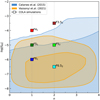 |
Fig. 1 Schematic representation of HS f(R) constraints in the fR0 − n plane. The coloured squares mark the locations of our simulations. The actual constraints at 1σ and 2σ confidence levels are taken from (Cataneo et al. 2015, blue contours) and (Vazsonyi et al. 2021, orange contours). |
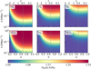 |
Fig. 2 Normalised effective gravitational constant of the HS model variants, as labelled in the respective panels. The colour intensity represents variations in Geff(k, a) across the scale factor, a, and Fourier modes, k. The dashed grey line corresponds to the redshift of interest in our simulations, i.e. z = 0.5. The colour bar indicates the intensity of deviation from the ΛCDM model. |
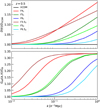 |
Fig. 4 Comparison of the normalised linear growth factors (upper panel) and effective gravitational constant (lower panel) of the MG models, as labelled. The variations in these quantities are shown as a function of k for the redshift of the simulations, z = 0.5. |
3 MG simulations and training dataset
We ran a set of high-resolution COLA simulations of ΛCDM and six HS models with |fR0| consistent with current constraints (see Sect. 2). The simulations were performed with the COLA Solver implemented in the publicly available FML library1, which succeeded MG-PICOLA. The FML-COLA solver extends the COLA method for simulating cosmological structure formation from ΛCDM to theories with scale-dependent growth such as the HS model. It also includes a fast approximate screening method described by Winther & Ferreira (2015). The simulated HS models correspond to six combinations of the exponent of the MG function, n, and the magnitude of the scalar field, |fR0|. These models correspond to the pairs (|fR0|, n) ∈ {(10−4, 1), (10−5, 1), (10−6, 1), (10−3.5, 2), (10−5, 2), (10−6.5, 2)}, which are denoted as {F41 F51, F61, F3.52, F52, F6.52}, respectively. The simulations are consistent with the best-fit parameters of Planck 2018 cosmology (Planck Collaboration VI 2020), and feature the dynamics of 20483 DM particles in a comoving box of 1 h−1 Gpc per side. The simulations commenced at z = 99, with initial conditions generated via a modified version of the 2LPTic code (Scoccimarro 1998; Crocce et al. 2006) implemented in FML. The HS models considered in this work share identical initial conditions with the ΛCDM run, as deviations in gravity are not expected at such a high redshift. The evolution of the DM particles extends up to redshift z = 0.5, comprising 100 time steps, which is a fairly large number. This finer temporal sampling allows a more detailed tracking of the evolution of the particle distribution, potentially capturing subtler effects in the simulation, albeit at the cost of increased computational resources.
Our setup ensures a mass resolution of Mp = 1.005 × 10¹⁰ h−1 M⊙ and a Nyquist frequency given by kNy = 6.43 h Mpc−1. Table 1 shows the key base cosmological parameters employed (left side) as well as the general setup of the COLA solver (right side). Table 2 presents the normalised effective gravitational constant and linear growth factors for various variants of the HS model at a redshift of z = 0.5. The Compton length and the corresponding wavenumber are provided for each model, indicating the characteristic scale at which the modifications to gravity become significant. As expected, the ![Mathematical equation: $\[\left.G_{\mathrm{eff}}\right|_{z=0.5 k=k_{\mathrm{C}}}\]$](/articles/aa/full_html/2024/10/aa50755-24/aa50755-24-eq12.png) ) remains approximately constant across all models, with a value of 1.33 ~ 4/3 at the characteristic scale. Similarly, the table illustrates that at the Compton scale, the impact of MG on the linear growth factor ratio is relatively small, with deviations from ΛCDM reaching up to 16%.
) remains approximately constant across all models, with a value of 1.33 ~ 4/3 at the characteristic scale. Similarly, the table illustrates that at the Compton scale, the impact of MG on the linear growth factor ratio is relatively small, with deviations from ΛCDM reaching up to 16%.
Dark matter halos were identified using the FoF algorithm, which connects particles within a distance of less than a specified linking length, b = 0.2, measured in units relative to the mean inter-particle distance (Davis et al. 1985). The linking length value has been shown to be valid for COLA simulations in previous works2 (see e.g. Howlett et al. 2015; Koda et al. 2016; Izard et al. 2016; Ferrero et al. 2021). We opted for the FoF halo finder over ROCKSTAR due to the poor performance of the later one when using COLA simulations (Fiorini et al. 2021). This finding is widely discussed by Fiorini et al. (2021), who show that the default ROCKSTAR settings can lead to statistical discrepancies in the halo properties when compared to N-body simulations, with differences of up to 25% in the halo mass function and approximately 10% variations in the power spectrum at k ~ 0.4 h Mpc−1. The reference catalogues used in this study refer to the halo distribution at z = 0.5 of each MG model plus ΛCDM as a benchmark model. We chose halos that contain no fewer than 80 DM particles, corresponding to an average mass-cut of FoF masses of MFoF ≳ 8 × 10¹¹ h−1 M⊙, which is represented by nearly ~3 × 10⁶ distinct halos per catalogue. This criterion agrees with the mass-cut employed in previous research to assess the performance of bias mapping methods (Vakili et al. 2017; Balaguera-Antolínez et al. 2019), as well as the mass-scale at which DM halos can host emission line galaxies in the extended Baryon Oscillation Spectroscopic Survey (eBOSS; for details, see Alam et al. 2020) and DESI-like galaxy samples (see Ding et al. 2022). Our mass-cut represents medium-mass halos that are above the threshold used by Ding et al. (2022) and Balaguera-Antolínez et al. (2024) and below the mass corresponding to the Sloan Digital Sky Survey-III BOSS CMASS galaxy catalogue (White et al. 2012; Dawson et al. 2013). We obtained DM fields from the particle distribution by applying a cloud-in-cell (CIC) mass assignment scheme to a N3 = 2563 mesh (equivalent to a resolution of 3.9 h−1 Mpc per cell). Halo number counts were obtained using a nearest-grid-point (NGP) scheme (Hockney & Eastwood 1981) and employing the same resolution as for the DM catalogues.
Figure 5 depicts the density field of DM particles (upper panels) and halos (bottom panels) at z = 0.5 in a region of 1000×1000×20 h−1 Mpc for the different gravity models considered in this work. The colour bar on the right gives the magnitude of the density perturbations. The white boxes show zoomed-in views, highlighting the similar web-like structures across these models despite the presence of MG effects. However, some differences are visible in the halo distribution, with some regions having a higher density of halos than in ΛCDM. These discrepancies stem from modifications in gravity, which amplify gravitational forces on small scales, thereby impacting the formation of prominent filaments, distinguished by either a significant thickness or a considerable length, along with a heightened abundance of halos. Such enhancements translate into a more pronounced abundance of rare and massive halos in the non-linear regime, as illustrated by cosmological simulations (Schmidt et al. 2009b).
Cosmological parameters employed in the COLA simulations along with key features of the simulation setup.
Normalised effective gravitational constant and linear growth factors of each variant of the HS model, evaluated at their respective Compton lengths and at the simulation redshift, z = 0.5.
4 BAM approach and calibration analysis
In this section we provide an overview of BAM, which we used to create the mock catalogues, along with the calibration conducted with the MG halo catalogues. We also present the summary statistics performance of the mapping for the different cosmologies. We refer the reader to Balaguera-Antolínez et al. (2023) for more details on the method.
4.1 Calibration: Kernel and halo bias
BAM is a non-parametric method designed to reproduce the halo number counts, Nh, of a reference catalogue within a mesh using a target DM density field. The idea behind the method consists of mapping the DM halo distribution by exploiting the concept of stochastic bias (Dekel & Lahav 1999; Somerville et al. 2001; Casas-Miranda et al. 2002), the minimisation of a cost function based on the power spectrum of target variables, and computing an iterative kernel that corrects for missing power towards small scales. The method has the capability of capturing the different properties of the halo bias by assuming that the number counts of halos in a volume cell depend on a set of properties of the DM density field evaluated in the same cells of volume ∂V. In this context, the bias is represented as a conditional probability distribution of the halo number counts, obtained directly from the reference simulation as a multi-dimensional histogram, ℬ (Nh | Θdm)∂V. The target DM density field can either be the one obtained from the full N-body snapshot downgraded to a mesh of N3 grid cells, or it can be generated by an approximate gravity solver that evolves the downgraded initial conditions of the N-body simulations in a mesh of the same dimensionality.
The calibration process, wherein the halo bias and a so-called BAM kernel are obtained solely from the two-point statistics of the reference catalogue as a target, involves an iterative procedure with the Markov chain Monte Carlo rejection algorithm. The aim of the BAM kernel is to adjust the DM density field through a convolution to match the reference tracer power spectrum. This process achieves approximately 1% accuracy in the power spectrum up to the Nyquist frequency, as demonstrated in previous studies (see e.g. Balaguera-Antolínez et al. 2019, 2020, 2023; Pellejero-Ibañez et al. 2020; Kitaura et al. 2022). The algorithm accounts for cross-correlations and other dependences, such as local and non-local properties like density and cosmic web type. We included them in the form of a cosmic-web classification (i.e. knots, filaments, sheets, and voids), which were obtained via the eigenvalues of the tidal field (see e.g. Hahn et al. 2007; Forero-Romero et al. 2009). The outputs of this procedure (halo-bias and kernel) enable the generation of new halo samples with the same probability density function (PDF) as the reference catalogue, representing the desired halo distribution. This mapping technique can then be applied to generate accurate halo distributions across various initial conditions while preserving the background cosmology.
4.2 Mapping MG cosmologies
We explored two calibration experiments to assess the performance of BAM in mapping MG cosmologies. The first consists of employing the MG DM fields to generate the corresponding MG halo number counts; this calibration is henceforth referred to as consistent-field calibration and can be represented by the following operation: ![Mathematical equation: $\[\delta_{\mathrm{DM}}^{\mathrm{MG}}\]$](/articles/aa/full_html/2024/10/aa50755-24/aa50755-24-eq13.png)

![Mathematical equation: $\[N_h^{\mathrm{MG}}\]$](/articles/aa/full_html/2024/10/aa50755-24/aa50755-24-eq14.png) where the operator indicates that the halo-bias relation from BAM has been applied to produce the mock catalogue. The second experiment, referred to as cross-field calibration from now on, consists of utilising the DM field of the ΛCDM model to generate the six different halo number counts of the MG HS models. The second calibration, represented by the transformation
where the operator indicates that the halo-bias relation from BAM has been applied to produce the mock catalogue. The second experiment, referred to as cross-field calibration from now on, consists of utilising the DM field of the ΛCDM model to generate the six different halo number counts of the MG HS models. The second calibration, represented by the transformation ![Mathematical equation: $\[\delta_{\mathrm{DM}}^{\Lambda \mathrm{CDM}}\]$](/articles/aa/full_html/2024/10/aa50755-24/aa50755-24-eq15.png)
![Mathematical equation: $\[N_h^{\mathrm{MG}}\]$](/articles/aa/full_html/2024/10/aa50755-24/aa50755-24-eq16.png) , is of interest because it allows us to create fast mocks of MG cosmologies without the need to run the corresponding MG simulations, which are usually computationally more expensive than the Λ DM ones.
, is of interest because it allows us to create fast mocks of MG cosmologies without the need to run the corresponding MG simulations, which are usually computationally more expensive than the Λ DM ones.
In terms of the effective field theory of large-scale structure, which in turn is based on cosmological perturbation theory, the transformations describing our two calibrations can be expressed as a linear superposition of fields, O, with corresponding bias coefficients ![Mathematical equation: $\[b_O\left(\tilde{b}_O\right)\]$](/articles/aa/full_html/2024/10/aa50755-24/aa50755-24-eq17.png) as well as stochastic contributions given by a field
as well as stochastic contributions given by a field ![Mathematical equation: $\[\epsilon(\tilde{\epsilon})\]$](/articles/aa/full_html/2024/10/aa50755-24/aa50755-24-eq18.png) and coefficients
and coefficients ![Mathematical equation: $\[c_{\epsilon, O}\left(\tilde{c}_{\tilde{\epsilon}, O}\right)\]$](/articles/aa/full_html/2024/10/aa50755-24/aa50755-24-eq19.png) (see e.g. Schmidt 2016; Desjacques et al. 2018). That is, the consistent-field calibration can be expressed as
(see e.g. Schmidt 2016; Desjacques et al. 2018). That is, the consistent-field calibration can be expressed as
![Mathematical equation: $\[\delta_h^{\mathrm{MG}}(\boldsymbol{x}, \tau)=\sum_O\left[b_O(\tau)+c_{\epsilon, O}(\tau) \epsilon(\boldsymbol{x}, \tau)\right] O\left[\delta_{\mathrm{DM}}^{\mathrm{MG}}\right](\boldsymbol{x}, \tau)+\epsilon(\boldsymbol{x}, \tau),\]$](/articles/aa/full_html/2024/10/aa50755-24/aa50755-24-eq20.png)
while for the cross-field calibration
![Mathematical equation: $\[\delta_h^{\mathrm{MG}}(\boldsymbol{x}, \tau)=\sum_O\left[\tilde{b}_O(\tau)+\tilde{c}_{\tilde{\epsilon}, O}(\tau) \tilde{\epsilon}(\boldsymbol{x}, \tau)\right] O\left[\delta_{\mathrm{DM}}^{\Lambda \mathrm{CDM}}\right](\boldsymbol{x}, \tau)+\tilde{\epsilon}(\boldsymbol{x}, \tau),\]$](/articles/aa/full_html/2024/10/aa50755-24/aa50755-24-eq21.png)
with x representing the position in space and τ being the time variable of the galaxy bias re-normalisation group. The tilde over the parameters in these expressions indicates their association with the cross-field calibration, distinguishing them from those in the consistent-field calibration.
BAM performs an iterative process aimed at mapping the DM field to the reference halos by minimising the two-point statistics, as previously discussed in Sect. 4.133. Figure 6 illustrates the different steps of the calibration process with a flowchart. Read from top to bottom, the process starts with the creation of initial conditions using 2LCTic, followed by the evolution of the DM particles with the COLA gravity solver until its distribution at z = 0.5 is obtained. Then, the FoF algorithm is applied to identify halo structures, whose number counts on the mesh are used as reference. The two branches of Fig. 6 distinguish the benchmark ΛCDM model from the MG models. The DM density fields and halo number counts are used as input in the BAM algorithm to perform the iterative process for producing a calibrated mock catalogue. The process ends with obtaining the BAM-kernel ![Mathematical equation: $\[\mathcal{K}\]$](/articles/aa/full_html/2024/10/aa50755-24/aa50755-24-eq23.png) or
or ![Mathematical equation: $\[\tilde{\mathcal{K}}\]$](/articles/aa/full_html/2024/10/aa50755-24/aa50755-24-eq24.png) as well as the corresponding bias relationship,
as well as the corresponding bias relationship, ![Mathematical equation: $\[\mathcal{B}\]$](/articles/aa/full_html/2024/10/aa50755-24/aa50755-24-eq25.png) or
or ![Mathematical equation: $\[\tilde{\mathcal{B}}\]$](/articles/aa/full_html/2024/10/aa50755-24/aa50755-24-eq26.png) , depending on the input DM density field, either ΛCDM or MG. Once the respective calibrations are obtained, we computed and compared the summary statistics, including density fields, PDFs, power spectra, and reduced bispectra4.
, depending on the input DM density field, either ΛCDM or MG. Once the respective calibrations are obtained, we computed and compared the summary statistics, including density fields, PDFs, power spectra, and reduced bispectra4.
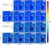 |
Fig. 5 Projected density field of DM and halos in a region of 1000×1000×20 h−3Mpc3 from seven different cosmologies at redshift z = 0.5. The upper panels display the DM density field and the lower panels the corresponding halo density field for the MG models, as labelled. These maps highlight the remarkable similarity in the density fields of MG and ΛCDM models. They also show that some models give rise to the formation of pronounced filaments, characterised by either a substantial thickness or a substantial length, as well as an increased prevalence of halos. |
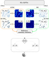 |
Fig. 6 Flowchart depicting the kernel and bias calibration using the COLA simulations as a reference to subsequently obtain the mapping bias relation, |
![Mathematical equation: $\[\tilde{\mathcal{B}}\]$](/articles/aa/full_html/2024/10/aa50755-24/aa50755-24-eq22.png)
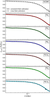 |
Fig. 7 Comparison of the cross-power spectrum between the mock catalogues generated with BAM and their respective reference catalogues for the two calibrations: consistent-field calibration (solid line) and cross-field calibration (dashed line). The colours of the dashed lines have the same meaning as in the other plots. |
4.3 Performance and summary statistics
In this section we present our main findings in terms of the summary statistics. Mapping the DM density fields with BAM provides the corresponding number counts of halos for each of the calibrations studied. Consequently, for each MG model, we generated two mock catalogues: one for the consistent-field calibration, denoted as ![Mathematical equation: $\[N_h^{\|}\]$](/articles/aa/full_html/2024/10/aa50755-24/aa50755-24-eq27.png) , and the other for the cross-field calibration, denoted as
, and the other for the cross-field calibration, denoted as ![Mathematical equation: $\[N_h^{\times}\]$](/articles/aa/full_html/2024/10/aa50755-24/aa50755-24-eq28.png) . The respective reference halo catalogue is labelled
. The respective reference halo catalogue is labelled ![Mathematical equation: $\[N_h^{\mathrm{ref}}\]$](/articles/aa/full_html/2024/10/aa50755-24/aa50755-24-eq29.png) . Firstly, we looked into the cross-power spectra between the references and the calibrated fields. Figure 7 shows the cross-power spectra of both calibration types across the MG cosmologies and ΛCDM. As seen in the figure, there are no significant fluctuations between the density fields in either calibration. In fact, the correlation exceeds 75% up to scales of k ~ 0.33 h Mpc−1 for all cosmologies. This indicates that the BAM kernel effectively captures the scale-dependent features of the growth factor that appear in the power spectrum of the MG models with high accuracy.
. Firstly, we looked into the cross-power spectra between the references and the calibrated fields. Figure 7 shows the cross-power spectra of both calibration types across the MG cosmologies and ΛCDM. As seen in the figure, there are no significant fluctuations between the density fields in either calibration. In fact, the correlation exceeds 75% up to scales of k ~ 0.33 h Mpc−1 for all cosmologies. This indicates that the BAM kernel effectively captures the scale-dependent features of the growth factor that appear in the power spectrum of the MG models with high accuracy.
Figure 8 displays the projected density field of the mock halo catalogues (right side of the sub-panels) in contrast to their respective reference (left side). The slices are shown for all cosmologies and the two calibrations, labelled as mocks from the consistent-field calibration (upper panels) and mocks from the cross-field calibration (bottom panels). Although both fields (reference and mock) are notably similar, some subtle differences can be appreciated within the circles highlighted in each subpanel. Nevertheless, in both sides of the panels, the large-scale structure is clearly consistent.
A qualitative analysis of Fig. 8 allows us to describe the region enclosed by the red circle in terms of its density variation compared to the reference catalogue. Overall, in the case of consistent-field calibration, ![Mathematical equation: $\[N_h^{\|}\]$](/articles/aa/full_html/2024/10/aa50755-24/aa50755-24-eq30.png) , all models except F52 exhibit a slight excess in density. The mock of ΛCDM shows no major deviations from its reference catalogue, which is consistent with previous analyses (see e.g. Balaguera-Antolínez et al. 2019, 2020; Pellejero-Ibañez et al. 2020; Kitaura et al. 2022). However, the mocks of the two extreme HS models, F41 and F3.52, which deviate significantly from GR gravity, display much higher density peaks compared to their references. Conversely, the F62 model is almost indistinguishable, with results comparable to those of Λ DM. Notably, density peaks in the mocks are particularly visible in knots and sheets. On the other hand, the mocks from the cross-field calibration,
, all models except F52 exhibit a slight excess in density. The mock of ΛCDM shows no major deviations from its reference catalogue, which is consistent with previous analyses (see e.g. Balaguera-Antolínez et al. 2019, 2020; Pellejero-Ibañez et al. 2020; Kitaura et al. 2022). However, the mocks of the two extreme HS models, F41 and F3.52, which deviate significantly from GR gravity, display much higher density peaks compared to their references. Conversely, the F62 model is almost indistinguishable, with results comparable to those of Λ DM. Notably, density peaks in the mocks are particularly visible in knots and sheets. On the other hand, the mocks from the cross-field calibration, ![Mathematical equation: $\[N_h^{\times}\]$](/articles/aa/full_html/2024/10/aa50755-24/aa50755-24-eq31.png) , exhibit a similar behaviour on large scales to those produced by the consistent calibration. However, in this case, when using the ΛCDM density field to generate MG mocks, the density peaks appear higher, particularly in the circled region used for comparison, compared to the consistent calibration. Specifically, the F3.52 model exhibits a slightly lower overdensity at the nodes compared to the previous calibration but remains distinguishable from the reference. Similarly, the F41 model displays a denser knot region than in the previous calibration, resulting in a significantly denser region than the reference catalogue. On the contrary, the F51 model shows comparable results in both calibrations, with no significant visual differences observed. The highlighted region in F52 shows an increase of two units in the density contrast, as indicated by the colour bar. Specifically, ρ/⟨ρ⟩ changes from 3 to 5 (equivalent to δ changing from 2 to 4), making it clearly distinguishable from the reference. Furthermore, F61 displays slightly denser regions in that area compared to the consistent-field calibration, making it easier to distinguish from ΛCDM. As in the previous model, F62 exhibits more power compared to the consistent calibration, resulting in clear differences from its reference catalogue despite being the closest model to ΛCDM in terms of clustering.
, exhibit a similar behaviour on large scales to those produced by the consistent calibration. However, in this case, when using the ΛCDM density field to generate MG mocks, the density peaks appear higher, particularly in the circled region used for comparison, compared to the consistent calibration. Specifically, the F3.52 model exhibits a slightly lower overdensity at the nodes compared to the previous calibration but remains distinguishable from the reference. Similarly, the F41 model displays a denser knot region than in the previous calibration, resulting in a significantly denser region than the reference catalogue. On the contrary, the F51 model shows comparable results in both calibrations, with no significant visual differences observed. The highlighted region in F52 shows an increase of two units in the density contrast, as indicated by the colour bar. Specifically, ρ/⟨ρ⟩ changes from 3 to 5 (equivalent to δ changing from 2 to 4), making it clearly distinguishable from the reference. Furthermore, F61 displays slightly denser regions in that area compared to the consistent-field calibration, making it easier to distinguish from ΛCDM. As in the previous model, F62 exhibits more power compared to the consistent calibration, resulting in clear differences from its reference catalogue despite being the closest model to ΛCDM in terms of clustering.
To evaluate the robustness of the calibrations with MG fields, we performed a comprehensive comparison of several summary statistics, including the PDF and the two- and three-point statistics of the halo distributions. We first compared the reference catalogues themselves, that is, the MG models against the ΛCDM model (i.e. ![Mathematical equation: $\[N_{h, \mathrm{MG}}^{\mathrm{ref}}\]$](/articles/aa/full_html/2024/10/aa50755-24/aa50755-24-eq32.png) versus
versus ![Mathematical equation: $\[N_{h, \Lambda \mathrm{CDM}}^{\mathrm{ref}}\]$](/articles/aa/full_html/2024/10/aa50755-24/aa50755-24-eq33.png) ), aiming to describe the specific signatures of the HS models in the summary statistics that distinguish them from the standard model. We then performed a similar comparison for the consistent-and cross-field calibrations, which correspond to
), aiming to describe the specific signatures of the HS models in the summary statistics that distinguish them from the standard model. We then performed a similar comparison for the consistent-and cross-field calibrations, which correspond to ![Mathematical equation: $\[N_{h, \mathrm{MG}}^{\|}\]$](/articles/aa/full_html/2024/10/aa50755-24/aa50755-24-eq34.png) versus
versus ![Mathematical equation: $\[N_{h, \Lambda \mathrm{CDM}}^{\|}\]$](/articles/aa/full_html/2024/10/aa50755-24/aa50755-24-eq35.png) and
and ![Mathematical equation: $\[N_{h, \mathrm{MG}}^{\times}\]$](/articles/aa/full_html/2024/10/aa50755-24/aa50755-24-eq36.png) versus
versus ![Mathematical equation: $\[N_{h, \Lambda \mathrm{CDM}}^{\times}\]$](/articles/aa/full_html/2024/10/aa50755-24/aa50755-24-eq37.png) , respectively. This analysis provides insights into the degree of physical information encoded within the bias relation
, respectively. This analysis provides insights into the degree of physical information encoded within the bias relation ![Mathematical equation: $\[\mathcal{B}~(\tilde{\mathcal{B}})\]$](/articles/aa/full_html/2024/10/aa50755-24/aa50755-24-eq38.png) provided by BAM. It allows us to ascertain the effectiveness of these mapping relations in accurately reproducing non-linear and non-local bias features, particularly in cosmologies characterised by scale-dependent growth factors. Figure 9 presents the outcomes of this analysis, with the mock comparison arranged from top to bottom as follows: reference catalogues only, consistent-field calibration, and cross-field calibration. The columns correspond, from left to right, to the PDF, power spectrum P(k), and reduced bispectrum, Q(θ12|k1, k2), in the particular configuration of k2 = 2k1 = 0.2 h Mpc−1. In this figure, all the ratios have been plotted with respect to the corresponding ΛCDM halo catalogue.
provided by BAM. It allows us to ascertain the effectiveness of these mapping relations in accurately reproducing non-linear and non-local bias features, particularly in cosmologies characterised by scale-dependent growth factors. Figure 9 presents the outcomes of this analysis, with the mock comparison arranged from top to bottom as follows: reference catalogues only, consistent-field calibration, and cross-field calibration. The columns correspond, from left to right, to the PDF, power spectrum P(k), and reduced bispectrum, Q(θ12|k1, k2), in the particular configuration of k2 = 2k1 = 0.2 h Mpc−1. In this figure, all the ratios have been plotted with respect to the corresponding ΛCDM halo catalogue.
The selected HS models are characterised by higher values of |fR0| that tend to manifest as more pronounced deviations from ΛCDM in terms of density fluctuations. Consequently, F41 exhibits more significant enhancements compared to its f51 and F61 counterparts. This trend arises from the fact that greater |fR0| values correspond to more substantial modifications to gravity, which consequently exert a more pronounced influence on the cosmic structure formation. In the first row of Fig. 9, we observe the expected behaviour in the summary statistics of the reference halos compared to the ΛCDM ones. Notably, the PDFs of MG models that feature significant gravity modifications, such as F3.52 and F41, exhibit an excess of probability of up to 20% of finding halos in cosmic environments whose overdensities are log(δh + 1) ≈ 1 and 1.5. This trend extends to models with moderate deviations from GR, such as F51 and F52, albeit for denser environments with log(δh + 1) ≈ 1.5 to 1.6. Conversely, models with weaker gravity modifications, such as F61 and F6.52, closely resemble the PDF of ΛCDM halos, with probability spreads below 2% even at higher densities. The PDF variations also manifest in the two-point statistics, particularly in the suppression of power in the low k modes. For instance, the suppression of power is better appreciated for F41 (exceeding 10%) compared to F3.52 (around 10%). Similarly, the F51 and F52 models show a more moderate power suppression, remaining below 5% for k < 0.08 h Mpc−1. As expected, the models with weak deviations from gravity, such as F61 and F62, display a consistent clustering across all scales when compared to ΛCDM. Moreover, an effective bias between the MG and ΛCDM models is observed for scales k > 0.1 h Mpc−1, with this bias monotonically increasing as the intensity of gravity deviation grows. As for the three-point statistic, the reduced bispectrum, Q(θ12), is also sensitive to modifications of gravity, as can be seen by the changes in its characteristic U-shape. In fact, the deeper the inflexion point, the more concave the bispectrum is, as seen for cosmologies with larger deviations from GR. In particular, when θ12 ≈ π/2, the F3.52 and F41 models exhibit deviations close to 20% compared to ΛCDM, the F51 and F52 models show deviations below 5%, and F61 and F62 closely resemble ΛCDM for the entire range of θ12 values.
The second and third rows of Fig. 9 show the summary statistics obtained from the consistent-field calibration, ![Mathematical equation: $\[\delta_{\mathrm{DM}}^{\mathrm{MG}}\]$](/articles/aa/full_html/2024/10/aa50755-24/aa50755-24-eq39.png)
![Mathematical equation: $\[N_h^{\mathrm{MG}}\]$](/articles/aa/full_html/2024/10/aa50755-24/aa50755-24-eq40.png) , and cross-field calibration,
, and cross-field calibration, ![Mathematical equation: $\[\delta_{\mathrm{DM}}^{\Lambda \mathrm{CDM}}\]$](/articles/aa/full_html/2024/10/aa50755-24/aa50755-24-eq41.png)
![Mathematical equation: $\[N_h^{\mathrm{MG}}\]$](/articles/aa/full_html/2024/10/aa50755-24/aa50755-24-eq42.png) , respectively. Analogous to the results of the reference catalogues (see the first row of Fig. 9), we focused on the mock quality regarding the signatures captured by the BAM bias relation with respect to the ΛCDM model rather than its reference catalogue, namely
, respectively. Analogous to the results of the reference catalogues (see the first row of Fig. 9), we focused on the mock quality regarding the signatures captured by the BAM bias relation with respect to the ΛCDM model rather than its reference catalogue, namely ![Mathematical equation: $\[N_{h, \mathrm{MG}}^{\|}\]$](/articles/aa/full_html/2024/10/aa50755-24/aa50755-24-eq43.png) versus
versus ![Mathematical equation: $\[N_{h, \Lambda \mathrm{CDM}}^{\|}\]$](/articles/aa/full_html/2024/10/aa50755-24/aa50755-24-eq44.png) and
and ![Mathematical equation: $\[N_{h, \mathrm{MG}}^{\times}\]$](/articles/aa/full_html/2024/10/aa50755-24/aa50755-24-eq45.png) versus
versus ![Mathematical equation: $\[N_{h, \Lambda \mathrm{CDM}}^{\times}\]$](/articles/aa/full_html/2024/10/aa50755-24/aa50755-24-eq46.png) .
.
First of all, we observe that the PDFs of all MG models remain identical in both calibrations, mirroring their respective reference catalogues. This consistency is an inherent feature of BAM. Moreover, the mocks of both calibration approaches reproduce the power spectrum of the reference catalogues beyond scales k ⩾ 0.1 h Mpc−1 remarkably well, as evidenced by the ratios of the power spectra. That is, the non-linear information encoded in Nh, MG is effectively captured by the bias relationship and BAM kernel of both calibrations. Below this scale (k < 1 h Mpc−1), however, we find deviations in the power spectrum of MG models, primarily attributed to cosmic variance stemming from the finite number of independent modes sampled within the grid volume. In this respect, the F3.52 and F41 mocks of the consistent-field calibration faithfully reflect the behaviour of the references on the largest scales. The remaining models become entangled within the cosmic variance, showing a clustering suppression ranging between approximately 4% and 8% in all cases, even in those models that closest resemble the ΛCDM field, such as F61 and F6.52. On the other hand, the power spectrum of the cross-field mocks aligns well with that of the references on large scales. Both families of models − F51, F5.52 and F61, F6.52 − show a closer resemblance to the clustering of the ΛCDM mock, while mocks from F3.52 and F41 exhibit noticeable deviations of up to 8%. However, it is worth noting that for F3.52 and F41, the BAM calibration tends to keep a consistent clustering suppression, unlike the characteristic patterns observed in the power spectrum of the reference catalogues (see the first row of Fig. 9). This result can be attributed to the fact that the BAM kernel primarily corrects clustering on non-linear scales rather than linear scales, where the power spectrum is expected to be easily mapped. At the same time, on these scales, the effects of MG become more significant in the power spectrum because, unlike on small scales where the chameleon mechanism is very efficient, here it tends to be weaker. Given that cosmic variance affects all models equally at the largest scales, we consistently observe the same hierarchy in the relative differences of the power spectrum compared to the ΛCDM mocks, that is to say, the features of MG are preserved with comparable accuracy to those of the original reference catalogues.
The last column of Fig. 9 shows the differences in the reduced bispectrum for both calibrations. Quantifying the discrepancies in the bispectrum proves challenges owing to the subtle deviations from ΛCDM observed in the reference catalogues. When translated to the calibrations, most of the deviations manifest in the depth of the U-shape around θ12 = π/2. Surprisingly, in both calibrations, the U-shape of models F51 and F61 is enhanced by an oscillating behaviour around the fiducial value set by ΛCDM. F3.52 and F41 mocks remain distinguishable in the two calibrations, although they do not follow the same trend as marked by the reference catalogues. The deviations in the bispectrum wings are within 5% for both consistent- and cross-field calibrations, which is in agreement with previous studies (see e.g. Gil-Marín et al. 2015; Pellejero-Ibañez et al. 2020; Kitaura et al. 2022). The reduced bispectrum indicates that while some of the MG features are not entirely recovered in the U-shape of the F51 and F61 models, the rest of MG models remain distinguishable from ΛCDM. Possible reasons for this include systematic errors in the BAM calibrations, resolution effects due to the employed grid size, and the intrinsic nature of the chameleon mechanism. Regarding the last factor, Gil-Marín et al. (2011) demonstrated the sensitivity of the reduced bispectrum to the chameleon mechanism, revealing substantial deviations between MG models and ΛCDM (up to 10–15%).
To move forward with our analysis and assess the mock quality and efficacy of the bias mapping of BAM in MG cosmologies, we compared the MG mocks to their corresponding reference catalogues, denoted as ![Mathematical equation: $\[N_{h, \mathrm{MG}}^{\|}\]$](/articles/aa/full_html/2024/10/aa50755-24/aa50755-24-eq47.png) versus
versus ![Mathematical equation: $\[N_{h, \mathrm{MG}}^{\mathrm{ref}}\]$](/articles/aa/full_html/2024/10/aa50755-24/aa50755-24-eq48.png) and
and ![Mathematical equation: $\[N_{h, \mathrm{MG}}^{\times}\]$](/articles/aa/full_html/2024/10/aa50755-24/aa50755-24-eq49.png) versus
versus ![Mathematical equation: $\[N_{h, \mathrm{MG}}^{\mathrm{ref}}\]$](/articles/aa/full_html/2024/10/aa50755-24/aa50755-24-eq50.png) . Previous studies (Balaguera-Antolínez et al. 2019, 2020; Pellejero-Ibañez et al. 2020; Kitaura et al. 2022) demonstrate that BAM achieves an accuracy of 1% or better in the power spectrum for ΛCDM simulations. Therefore, our comparison is particularly insightful as it allows us to evaluate BAM’s accuracy at reproducing the halo distribution in a new scenario, namely using MG cosmologies. In that regard, Fig. 10 shows the power spectrum and bispectrum of the MG mocks for both the consistent-field calibration (upper panels) and cross-field calibration (lower panels). Both the power spectra and bispectra curves have been shifted for clarity. Note that the ΛCDM model is special, as its statistics remain the same in both calibrations. The two calibrations (consistent- and cross-field calibration) show excellent agreement with the reference power spectrum, with residuals between the mock power spectra and the reference one within 1% up to k ~ 0.8 h−1 Mpc. This precision underscores the importance of considering both local and nonlocal properties of the reference catalogue (Kitaura et al. 2022; Balaguera-Antolínez et al. 2024).
. Previous studies (Balaguera-Antolínez et al. 2019, 2020; Pellejero-Ibañez et al. 2020; Kitaura et al. 2022) demonstrate that BAM achieves an accuracy of 1% or better in the power spectrum for ΛCDM simulations. Therefore, our comparison is particularly insightful as it allows us to evaluate BAM’s accuracy at reproducing the halo distribution in a new scenario, namely using MG cosmologies. In that regard, Fig. 10 shows the power spectrum and bispectrum of the MG mocks for both the consistent-field calibration (upper panels) and cross-field calibration (lower panels). Both the power spectra and bispectra curves have been shifted for clarity. Note that the ΛCDM model is special, as its statistics remain the same in both calibrations. The two calibrations (consistent- and cross-field calibration) show excellent agreement with the reference power spectrum, with residuals between the mock power spectra and the reference one within 1% up to k ~ 0.8 h−1 Mpc. This precision underscores the importance of considering both local and nonlocal properties of the reference catalogue (Kitaura et al. 2022; Balaguera-Antolínez et al. 2024).
The precision achieved in the power spectra ratios of the consistent-field calibration is expected, given that the halo distribution inherits the non-linear and non-local properties of the respective MG DM density field. Therefore, it is not surprising that the range of accuracy is broader in this calibration, as depicted in Fig. 10. Regarding the cross-field calibration, we observe the anticipated deviations in the power spectrum at large scales, arising from the lack of power of the MG models compared to ΛCDM, as previously discussed with Fig. 9. The discrepancies in the power spectrum of the MG mocks at scales below k < 0.07 h Mpc−1 are due to the convergence phase of the bias method, not specific MG features of the HS models. Since BAM works as a Markov chain Monte Carlo method, some differences between different calibrations can be expected regardless of the MG model, especially on large scales where cosmic variance in the form of a low number of Fourier modes is important. In particular, we notice that the suppression of power in the halo distribution of the F3.52 and F41 mocks manifests in the lower panels of Fig. 10 as a bump in power at the same scales. Similarly, the mocks for F51 and F5.52 exhibit an excess in power of approximately 10% at scales k ≈ 0.02 h Mpc−1. The residuals between the P(k) of F61 and F6.52 and their references are within 5%, even at the largest scales, closely resembling the behaviour of the ΛCDM halos; this is a good indicator that even when calibrations are performed using crossed DM fields, it is feasible to derive statistics of the MG halo distribution. By analysing the three-point statistics of the consistent-field calibration, we observe a U-shaped pattern in the residuals of the bispectra of the mocks. This indicates a better fit at the inflexion point, while improvement is desirable on the wings. However, this shape is much reduced in the cross-field calibration, which is due to a minor increase in the agreement of the inflexion point, while the fit of the wings stays consistent between calibrations. Our findings show that the mock of F3.52 in the cross-field calibration improves the inflexion point somewhat compared to the consistent-field calibration, while residuals remain within 10% in both calibrations. Likewise, the F41 mocks exhibit minimal deviation in the bispectra residuals, with both calibrations showing consistency within 10% across most of the θ12 range. Mocks of the F51 model do show a slight improvement at θ12 ≈ π/2, but this improvement holds true for both calibrations. As compared to the cross-field calibration, the mocks of F52 show improved agreement in consistent-field calibration across the entire θ12 range, reducing deviations by over 10%. Last but not least, the mocks of F61 and F6.52 cosmologies show good agreement with their reference catalogues in both calibrations, with only one point deviating at θ12 ≈ 1.8.
The analysis of the reduced bispectrum in HS models uncovers deviations of up to 10–15% compared to ΛCDM, highlighting its potential to discern between MG models. In particular, MG casts a weaker influence on the bispectrum than on the power spectrum, suggesting its utility in breaking galaxy-bias degeneracies. The bispectrum, as a measurement of the raw amplitude of three-point correlations, has also been studied in the past for HS f(R) models (see Alam et al. 2021). Our results show agreement with previous studies of the reduced bispectrum, particularly with Gil-Marín et al. (2011), who used a similar setup of the N-body simulations, which employed the same initial conditions across all the MG models. The findings indicate that differences in the bispectrum are naturally inherited from the power spectrum; however, the sensitivity to capture the gravitational signatures of the f(R) model is only visible at the percent level, as theoretically studied by Borisov & Jain (2009). Similar analyses of the reduced bispectrum with COLA simulations (see Fiorini et al. 2022) support this statement. The consistent differences observed in both the power spectrum and the bispectrum emphasise the critical importance of accurate measurements for model constraints. The bispectrum provides a valuable diagnostic tool for delineating MG effects and warrants further exploration through various parameter combinations to maximise the signal-to-noise ratio. It is worth noting that within our analysis, the bispectrum is not a calibrated quantity in the BAM approach, which underscores that the observed agreement, as shown in Fig. 10, is naturally inherited from the local and non-local properties of the density fields used in the multi-dimensional halo bias described in Sec. 4.
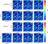 |
Fig. 8 Projected density field in slices of 240 × 500 × 98 h−3 Mpc3 from a volume of 10003 h−3Mpc3 of the reference and mock catalogues for all cosmologies. Upper panels: Mocks from the consistent-field calibration. Bottom panels: Mocks from the cross-field calibration. Each sub-panel is divided in two; the left side corresponds to the reference halos from the N-body simulation and the right side to their respective mock obtained with BAM. The models are as labelled, and the colour bar indicates the density 1 + δh. Note that the ΛCDM model is a particular case in which the mock is the same in both the upper and lower panels, as it serves as the reference model. The circles in each panel display a region of interest where visual differences in overdensity are visible to the naked eye (dashed circle for reference halos and solid circle for mocks). |
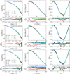 |
Fig. 9 Comparison of the PDFs (left), power spectra (P(k); middle), and reduced bispectra (Q(k1, k2, θ12); right) from the calibration stage obtained with BAM for the different MG models, as labelled. Upper panels: reference halo catalogues. Middle row: mock calibration created with BAM from the consistent MG DM field of each model. Lower row: mock calibration created with BAM from the DM field of the ΛCDM model. Note that all the comparisons are made between the MG model with respect to the ΛCDM field. |
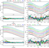 |
Fig. 10 Power spectrum and reduced bispectrum of the different MG mocks (dashed lines) compared to their respective reference catalogues (solid lines) for the studied calibrations, as labelled. Upper panels: consistent-field calibration, i.e. |
![Mathematical equation: $\[N_{h, \mathrm{MG}}^{\|}\]$](/articles/aa/full_html/2024/10/aa50755-24/aa50755-24-eq51.png)
![Mathematical equation: $\[N_{h, \mathrm{MG}}^{\mathrm{ref}}\]$](/articles/aa/full_html/2024/10/aa50755-24/aa50755-24-eq52.png)
![Mathematical equation: $\[N_{h, \mathrm{MG}}^{\times}\]$](/articles/aa/full_html/2024/10/aa50755-24/aa50755-24-eq53.png)
![Mathematical equation: $\[N_{h, \mathrm{MG}}^{\mathrm{ref}}\]$](/articles/aa/full_html/2024/10/aa50755-24/aa50755-24-eq54.png)
5 Summary and discussion
This study focuses on efficiently generating MG catalogues from mapping either standard or MG-DM density fields using BAM. Our results assess the flexibility of BAM in effectively modelling the effects of MG using a benchmark training data catalogue, by incorporating non-local and non-linear information into the description of halo bias. The analysis was conducted across six distinct cosmologies based on the HS parametrisation (Hu & Sawicki 2007) of the f(R) gravity model. These cosmologies encompass various levels of deviation from the ΛCDM model, including those capable of mimicking the clustering of ΛCDM and those with significant deviations that have already been ruled out by Solar System constraints. One important component of our study is the exploration of the growth factor and effective gravitational constant for different configurations of the power-law index, n, and the magnitude of the scalar field, |fR0|, of the MG models. Both the scale-dependent growth factor and variations in gravity are crucial for understanding bias relations in MG models. Therefore, we focused on the redshift z = 0.5 to align with recent galaxy survey data and span a wide range of k modes in Fourier space, providing comprehensive coverage across both large and small scales. In particular, we considered the distribution of DM halos generated in different MG models generated with COLA and used BAM to obtain non-parametric bias relations for each MG model. We employed two distinct calibration experiments, namely consistent-field and cross-field calibrations. In the consistent-field calibration, we used the DM of MG models to mimic the corresponding MG catalogues, ensuring self-consistency between DM and number counts of biased tracers. This approach is expected to effectively capture most of the MG effects in the bias relation. Conversely, the cross-field calibration offers the opportunity to rapidly generate mock MG catalogues by using a mapping relationship based on the DM density field of a ΛCDM simulation rather than running MG simulations, which are typically more demanding.
We employed the two- and three-point statistics to assess the effectiveness of the mapping relations obtained with our non-parametric approach. It should be stressed that during the calibration process, the one-point statistic, namely the PDF, is adjusted to match the desired number counts, in our case those of the MG models. In the meantime, the power spectrum was computed for each iteration, during which the DM was convolved with the BAM kernel until it reached sufficient accuracy to reproduce the target power spectrum of the MG halos. It is noteworthy that the three-point statistic is not directly involved in the calibration process; therefore, the results obtained reflect the amount of information in the non-linear and non-local information of the density field (see e.g. Balaguera-Antolínez et al. 2019, 2020; Kitaura et al. 2022; Bartlett et al. 2024). Our results demonstrate that the MG halos obtained from both calibrations excel in summary statistics, achieving a 1% accuracy in the power spectrum from k = 0.1 h Mpc−1 up to the Nyquist frequency. The accuracy is below 5% in the range k = 0.1–0.3 h Mpc−1, with minimal differences well below 5% at low modes. However, larger deviations can occur at the smallest k modes, around 10%, depending on the specific model. Meanwhile, the bispectrum remains consistent with the reference catalogues within 15% for all values of the θ12 angle in the typical configuration k2 = 2k1 = 0.2 h Mpc−1. However, model-specific discrepancies for each MG cosmology become apparent when examining bispectrum values below 5%, which reveals more intricate behaviour that, in general, depends on the complex growth of structure in these models, as detailed in Sec. 4.3.
The analysis of BAM calibrations reveals that the consistent-field calibration has a good accuracy over broader ranges, showcasing the non-linear and non-local properties inherited from the MG DM density fields. In contrast, the cross-field calibration displays the predicted deviations on large scales due to differences in power between MG models and the standard ΛCDM model. Specific features of the HS parametrisations led to deviations in the power spectrum (with some models showing a suppression thereof), especially at large scales. Moreover, deviations of up to 10–15% in the reduced bispectrum compared to ΛCDM highlight the potential of this statistic to distinguish between MG models and its potential in breaking galaxy-bias degeneracies. The consistent-field calibration shows a U-shaped pattern in bispectrum residuals, indicating that a better fit at the inflexion point is desirable; there is also room for improvement on the wings. The cross-field calibration, on the other hand, exhibits flat ratios, with a consistent wing fit across calibrations.
The precision achieved when using MG reference catalogues demonstrates the competitive capability of non-parametric architectures, such as BAM, in generating mocks from DM fields, whether it is ΛCDM or MG. In fact, learning complex bias relations is essential for generating mock catalogues that faithfully reproduce the halo number counts and statistical features of cosmologies beyond ΛCDM, facilitating further cosmo-logical analysis. As mentioned before, a key factor that allows us to achieve unprecedented accuracy is the inclusion of non-linear and non-local information from the reference training dataset via the cosmic web classification. In the MG context, this is even more relevant due to the nature of the chameleon mechanism, which operates in high-density environments by suppressing modifications to gravity while allowing significant modifications on cosmological scales. This highlights the fact that the HS scalar field leads to an amplified growth of structures on large scales, resulting in higher-density peaks compared to the ΛCDM model. In contrast, on smaller scales, these modifications tend to decrease structure formation, leading to a smoother density field. Indeed, in dense environments such as clusters, the chameleon mechanism operates efficiently, leading to suppressed gravity modifications. On the other hand, in under-dense regions such as voids, the chameleon mechanism is ineffective, resulting in significant modifications to gravity. Li et al. (2012a) demonstrate that this environmental dependence serves as strong evidence for gravity modification in models that feature the chameleon mechanism. Thus, by employing a non-linear and non-local bias description, our results confirm that the effects of MG can be effectively captured when environmental information of the DM density field is provided.
Overall, this approach enhances the representation of the matter distribution in alternative cosmological scenarios, with diverse structure formation and gravitational effects across different scales. The results indicate that summary statistics, including power spectra and reduced bispectrum, align with the reference catalogues for various MG models. This suggests that BAM accurately reproduces the clustering patterns and deviations caused by MG, providing valuable insights for future cosmological analyses. Looking ahead, we plan to assess the impact of different MG models on the scaling relations of the properties of DM halos and their correlations with the large-scale effective primary and secondary bias (Balaguera-Antolínez et al. 2024). We will also apply the parametric mapping technique (Coloma-Nadal et al. 2024) to each of the different regions of a novel hierarchical cosmic web classification. These developments and insights into the clustering in non-standard cosmologies promise to further refine the MG mock catalogue generation process and will be useful in the context of testing gravity in surveys such as Euclid, DESI, and LSST.
Acknowledgements
We would like to thank Ismael Ferrero, Farbod Hassani, David Mota and Hans Winther for discussions in the early stage of this project. The authors acknowledge support from the Canarian government under the project “Mapping the Universe with modified gravity” PROID2021010126, and the Spanish Ministry of Economy and Competitiveness (MINECO) for financing the Big Data of the Cosmic Web project: PID2020-120612GB-I00/AEI/10.13039/501100011033, and the IAC for continuous support to the Cosmology with LSS probes project. J.E.G.F. is supported by the Spanish Ministry of Universities, through a María Zambrano grant (program 2021–2023) at Universidad de La Laguna with reference UP2021-022, funded within the European Union-Next Generation EU. A.B.A. acknowledges the Spanish Ministry of Economy and Competitiveness (MINECO) under the Severo Ochoa program SEV-2015-0548 grants. We also thank the personnel of the Servicios Informáticos Comunes (SIC) of the IAC.
References
- Alam, S., Peacock, J. A., Kraljic, K., Ross, A. J., & Comparat, J. 2020, MNRAS, 497, 581 [NASA ADS] [CrossRef] [Google Scholar]
- Alam, S., Arnold, C., Aviles, A., et al. 2021, JCAP, 2021, 050 [Google Scholar]
- Angulo, R. E., & White, S. D. M. 2010, MNRAS, 405, 143 [NASA ADS] [Google Scholar]
- Angulo, R. E., Baugh, C. M., Frenk, C. S., & Lacey, C. G. 2014, MNRAS, 442, 3256 [NASA ADS] [CrossRef] [Google Scholar]
- Arnalte-Mur, P., Hellwing, W. A., & Norberg, P. 2017, MNRAS, 467, 1569 [NASA ADS] [Google Scholar]
- Arnold, C., & Li, B. 2019, MNRAS, 490, 2507 [NASA ADS] [CrossRef] [Google Scholar]
- Arnold, C., Li, B., Giblin, B., Harnois-Déraps, J., & Cai, Y.-C. 2022, MNRAS, 515, 4161 [CrossRef] [Google Scholar]
- Avila, S., Murray, S. G., Knebe, A., et al. 2015, MNRAS, 450, 1856 [NASA ADS] [CrossRef] [Google Scholar]
- Balaguera-Antolínez, A., Kitaura, F.-S., Pellejero-Ibáñez, M., Zhao, C., & Abel, T. 2019, MNRAS, 483, L58 [CrossRef] [Google Scholar]
- Balaguera-Antolínez, A., Kitaura, F.-S., Pellejero-Ibáñez, M., et al. 2020, MNRAS, 491, 2565 [Google Scholar]
- Balaguera-Antolínez, A., Kitaura, F.-S., Alam, S., et al. 2023, A&A, 673, A130 [NASA ADS] [CrossRef] [EDP Sciences] [Google Scholar]
- Balaguera-Antolínez, A., Montero-Dorta, A. D., & Favole, G. 2024, A&A, 685, A61 [NASA ADS] [CrossRef] [EDP Sciences] [Google Scholar]
- Bartlett, D. J., Ho, M., & Wandelt, B. D. 2024, arXiv e-prints [arXiv:2405.00635] [Google Scholar]
- Bel, J., Brax, P., Marinoni, C., & Valageas, P. 2015, Phys. Rev. D, 91, 103503 [NASA ADS] [CrossRef] [Google Scholar]
- Berlind, A. A., Weinberg, D. H., Benson, A. J., et al. 2003, ApJ, 593, 1 [NASA ADS] [CrossRef] [Google Scholar]
- Bond, J. R., & Myers, S. T. 1996, ApJS, 103, 1 [NASA ADS] [CrossRef] [Google Scholar]
- Borisov, A., & Jain, B. 2009, Phys. Rev. D, 79, 103506 [NASA ADS] [CrossRef] [Google Scholar]
- Boubekeur, L., Giusarma, E., Mena, O., & Ramírez, H. 2014, Phys. Rev. D, 90, 103512 [CrossRef] [Google Scholar]
- Brando, G., Fiorini, B., Koyama, K., & Winther, H. A. 2022, J. Cosmology Astropart. Phys., 2022, 051 [CrossRef] [Google Scholar]
- Capozziello, S., & de Laurentis, M. 2011, Phys. Rep., 509, 167 [CrossRef] [Google Scholar]
- Carretero, J., Castander, F. J., Gaztañaga, E., Crocce, M., & Fosalba, P. 2015, MNRAS, 447, 646 [NASA ADS] [CrossRef] [Google Scholar]
- Casas, S., Cardone, V. F., Sapone, D., et al. 2023, A&A, in press https://doi.org/10.1051/0004-6361/202448713 [Google Scholar]
- Casas-Miranda, R., Mo, H. J., Sheth, R. K., & Boerner, G. 2002, MNRAS, 333, 730 [NASA ADS] [CrossRef] [Google Scholar]
- Cataneo, M., Rapetti, D., Schmidt, F., et al. 2015, Phys. Rev. D, 92, 044009 [NASA ADS] [CrossRef] [Google Scholar]
- Chuang, C.-H., Kitaura, F.-S., Prada, F., Zhao, C., & Yepes, G. 2015, MNRAS, 446, 2621 [NASA ADS] [CrossRef] [Google Scholar]
- Coloma-Nadal, J. M., Kitaura, F. S., García-Farieta, J. E., et al. 2024, J. Cosmol. Astropart. Phys., 2024, 083 [CrossRef] [Google Scholar]
- Contreras, S., Angulo, R. E., Zennaro, M., Aricò, G., & Pellejero-Ibañez, M. 2020, MNRAS, 499, 4905 [Google Scholar]
- Crocce, M., Pueblas, S., & Scoccimarro, R. 2006, MNRAS, 373, 369 [NASA ADS] [CrossRef] [Google Scholar]
- Davis, M., Efstathiou, G., Frenk, C. S., & White, S. D. M. 1985, ApJ, 292, 371 [Google Scholar]
- Dawson, K. S., Schlegel, D. J., Ahn, C. P., et al. 2013, AJ, 145, 10 [Google Scholar]
- De Felice, A., & Tsujikawa, S. 2010, Liv. Rev. Relativ., 13, 3 [NASA ADS] [CrossRef] [Google Scholar]
- Dekel, A., & Lahav, O. 1999, ApJ, 520, 24 [Google Scholar]
- DESI Collaboration (Aghamousa, A., et al.) 2016, arXiv e-prints [arXiv:1611.00036] [Google Scholar]
- Desjacques, V., Jeong, D., & Schmidt, F. 2018, Phys. Rep., 733, 1 [Google Scholar]
- Ding, Z., Chuang, C.-H., Yu, Y., et al. 2022, MNRAS, 514, 3308 [CrossRef] [Google Scholar]
- Esposito-Farèse, G., & Polarski, D. 2001, Phys. Rev. D, 63, 063504 [CrossRef] [Google Scholar]
- Feng, Y., Chu, M.-Y., Seljak, U., & McDonald, P. 2016, MNRAS, 463, 2273 [NASA ADS] [CrossRef] [Google Scholar]
- Ferrero, I., Crocce, M., Tutusaus, I., et al. 2021, A&A, 656, A106 [NASA ADS] [CrossRef] [EDP Sciences] [Google Scholar]
- Fiorini, B., Koyama, K., Izard, A., et al. 2021, JCAP, 2021, 021 [Google Scholar]
- Fiorini, B., Koyama, K., & Izard, A. 2022, JCAP, 2022, 028 [CrossRef] [Google Scholar]
- Forero-Romero, J. E., Hoffman, Y., Gottlöber, S., Klypin, A., & Yepes, G. 2009, MNRAS, 396, 1815 [Google Scholar]
- García-Farieta, J. E., Marulli, F., Veropalumbo, A., et al. 2019, MNRAS, 488, 1987 [Google Scholar]
- García-Farieta, J. E., Hellwing, W. A., Gupta, S., & Bilicki, M. 2021, Phys. Rev. D, 103, 103524 [CrossRef] [Google Scholar]
- Gil-Marín, H., Schmidt, F., Hu, W., Jimenez, R., & Verde, L. 2011, JCAP, 2011, 019 [CrossRef] [Google Scholar]
- Gil-Marín, H., Noreña, J., Verde, L., et al. 2015, MNRAS, 451, 539 [CrossRef] [Google Scholar]
- Gordon, J., de Aguiar, B. F., Rebouças, J., et al. 2024, arXiv e-prints [arXiv:2404.12344] [Google Scholar]
- Gupta, S., Hellwing, W. A., Bilicki, M., & García-Farieta, J. E. 2022, Phys. Rev. D, 105, 043538 [NASA ADS] [CrossRef] [Google Scholar]
- Gupta, S., Hellwing, W. A., & Bilicki, M. 2023, Phys. Rev. D, 107, 083525 [CrossRef] [Google Scholar]
- Hahn, O., Porciani, C., Carollo, C. M., & Dekel, A. 2007, MNRAS, 375, 489 [NASA ADS] [CrossRef] [Google Scholar]
- He, J.-h., Li, B., & Jing, Y. P. 2013, Phys. Rev. D, 88, 103507 [CrossRef] [Google Scholar]
- Hernández-Aguayo, C., Baugh, C. M., & Li, B. 2018, MNRAS, 479, 4824 [CrossRef] [Google Scholar]
- Hernández-Aguayo, C., Hou, J., Li, B., Baugh, C. M., & Sánchez, A. G. 2019, MNRAS, 485, 2194 [CrossRef] [Google Scholar]
- Hikage, C., Oguri, M., Hamana, T., et al. 2019, PASJ, 71, 43 [Google Scholar]
- Hockney, R. W., & Eastwood, J. W. 1981, Computer Simulation Using Particles (Boca Raton: CRC Press) [Google Scholar]
- Howlett, C., Ross, A. J., Samushia, L., Percival, W. J., & Manera, M. 2015, MNRAS, 449, 848 [NASA ADS] [CrossRef] [Google Scholar]
- Hu, W., & Sawicki, I. 2007, Phys. Rev. D, 76, 064004 [CrossRef] [Google Scholar]
- Ivarsen, M. F., Bull, P., Llinares, C., & Mota, D. 2016, A&A, 595, A40 [NASA ADS] [CrossRef] [EDP Sciences] [Google Scholar]
- Izard, A., Crocce, M., & Fosalba, P. 2016, MNRAS, 459, 2327 [NASA ADS] [CrossRef] [Google Scholar]
- Jain, B., Vikram, V., & Sakstein, J. 2013, ApJ, 779, 39 [NASA ADS] [CrossRef] [Google Scholar]
- Jennings, E., Baugh, C. M., Li, B., Zhao, G.-B., & Koyama, K. 2012, MNRAS, 425, 2128 [NASA ADS] [CrossRef] [Google Scholar]
- Joyce, A., Lombriser, L., & Schmidt, F. 2016, Ann. Rev. Nucl. Part. Sci., 66, 95 [NASA ADS] [CrossRef] [Google Scholar]
- Khoury, J., & Weltman, A. 2004a, Phys. Rev. D, 69, 044026 [CrossRef] [Google Scholar]
- Khoury, J., & Weltman, A. 2004b, Phys. Rev. Lett., 93, 171104 [NASA ADS] [CrossRef] [Google Scholar]
- Kitaura, F. S., Yepes, G., & Prada, F. 2014, MNRAS, 439, L21 [NASA ADS] [CrossRef] [Google Scholar]
- Kitaura, F.-S., Gil-Marín, H., Scóccola, C. G., et al. 2015, MNRAS, 450, 1836 [NASA ADS] [CrossRef] [Google Scholar]
- Kitaura, F.-S., Rodríguez-Torres, S., Chuang, C.-H., et al. 2016, MNRAS, 456, 4156 [NASA ADS] [CrossRef] [Google Scholar]
- Kitaura, F.-S., Ata, M., Rodríguez-Torres, S. A., et al. 2021, MNRAS, 502, 3456 [NASA ADS] [CrossRef] [Google Scholar]
- Kitaura, F. S., Balaguera-Antolínez, A., Sinigaglia, F., & Pellejero-Ibáñez, M. 2022, MNRAS, 512, 2245 [NASA ADS] [CrossRef] [Google Scholar]
- Kitaura, F. S., Sinigaglia, F., Balaguera-Antolínez, A., & Favole, G. 2024, A&A, 683, A215 [NASA ADS] [CrossRef] [EDP Sciences] [Google Scholar]
- Kobayashi, T. 2019, Rep. Prog. Phys., 82, 086901 [NASA ADS] [CrossRef] [Google Scholar]
- Koda, J., Blake, C., Beutler, F., Kazin, E., & Marin, F. 2016, MNRAS, 459, 2118 [NASA ADS] [CrossRef] [Google Scholar]
- Laureijs, R., Amiaux, J., Arduini, S., et al. 2011, arXiv e-prints [arXiv:1110.3193] [Google Scholar]
- L’Huillier, B., Winther, H. A., Mota, D. F., Park, C., & Kim, J. 2017, MNRAS, 468, 3174 [Google Scholar]
- Li, B., Zhao, G.-B., & Koyama, K. 2012a, MNRAS, 421, 3481 [NASA ADS] [CrossRef] [Google Scholar]
- Li, B., Zhao, G.-B., Teyssier, R., & Koyama, K. 2012b, J. Cosmology Astropart. Phys., 2012, 051 [CrossRef] [Google Scholar]
- Li, B., Hellwing, W. A., Koyama, K., et al. 2013, MNRAS, 428, 743 [CrossRef] [Google Scholar]
- Liu, R., Valogiannis, G., Battaglia, N., & Bean, R. 2021, Phys. Rev. D, 104, 103519 [NASA ADS] [CrossRef] [Google Scholar]
- Llinares, C., & Mota, D. F. 2014, Phys. Rev. D, 89, 084023 [NASA ADS] [CrossRef] [Google Scholar]
- Lombriser, L. 2014, Annalen der Physik, 264, 259 [CrossRef] [Google Scholar]
- Manera, M., Scoccimarro, R., Percival, W. J., et al. 2013, MNRAS, 428, 1036 [Google Scholar]
- Manera, M., Samushia, L., Tojeiro, R., et al. 2015, MNRAS, 447, 437 [NASA ADS] [CrossRef] [Google Scholar]
- Mead, A. J., Peacock, J. A., Lombriser, L., & Li, B. 2015, MNRAS, 452, 4203 [NASA ADS] [CrossRef] [Google Scholar]
- Monaco, P., Theuns, T., & Taffoni, G. 2002, MNRAS, 331, 587 [Google Scholar]
- Mota, D. F., & Shaw, D. J. 2007, Phys. Rev. D, 75, 063501 [NASA ADS] [CrossRef] [Google Scholar]
- Oyaizu, H., Lima, M., & Hu, W. 2008, Phys. Rev. D, 78, 123524 [NASA ADS] [CrossRef] [Google Scholar]
- Pellejero-Ibañez, M., Balaguera-Antolínez, A., Kitaura, F.-S., et al. 2020, MNRAS, 493, 586 [CrossRef] [Google Scholar]
- Planck Collaboration VI. 2020, A&A, 641, A6 [NASA ADS] [CrossRef] [EDP Sciences] [Google Scholar]
- Pogosian, L., & Silvestri, A. 2008, Phys. Rev. D, 77, 023503 [NASA ADS] [CrossRef] [Google Scholar]
- Ramachandra, N., Valogiannis, G., Ishak, M., Heitmann, K., & LSST Dark Energy Science Collaboration. 2021, Phys. Rev. D, 103, 123525 [CrossRef] [Google Scholar]
- Ruan, C.-Z., Cuesta-Lazaro, C., Eggemeier, A., et al. 2024, MNRAS, 527, 2490 [Google Scholar]
- Schmidt, F. 2016, Phys. Rev. D, 93, 063512 [NASA ADS] [CrossRef] [Google Scholar]
- Schmidt, F., Lima, M., Oyaizu, H., & Hu, W. 2009a, Phys. Rev. D, 79, 083518 [NASA ADS] [CrossRef] [Google Scholar]
- Schmidt, F., Vikhlinin, A., & Hu, W. 2009b, Phys. Rev. D, 80, 083505 [NASA ADS] [CrossRef] [Google Scholar]
- Scoccimarro, R. 1998, MNRAS, 299, 1097 [NASA ADS] [CrossRef] [Google Scholar]
- Scoccimarro, R., & Sheth, R. K. 2002, MNRAS, 329, 629 [NASA ADS] [CrossRef] [Google Scholar]
- Shirasaki, M., Hamana, T., & Yoshida, N. 2016, PASJ, 68, 4 [NASA ADS] [CrossRef] [Google Scholar]
- Smith, R. E., Peacock, J. A., Jenkins, A., et al. 2003, MNRAS, 341, 1311 [Google Scholar]
- Somerville, R. S., Lemson, G., Sigad, Y., et al. 2001, MNRAS, 320, 289 [Google Scholar]
- Sotiriou, T. P., & Faraoni, V. 2010, Rev. Mod. Phys., 82, 451 [NASA ADS] [CrossRef] [Google Scholar]
- Tassev, S., Zaldarriaga, M., & Eisenstein, D. J. 2013, JCAP, 6, 036 [CrossRef] [Google Scholar]
- Tsujikawa, S., Uddin, K., Mizuno, S., Tavakol, R., & Yokoyama, J. 2008, Phys. Rev. D, 77, 103009 [NASA ADS] [CrossRef] [Google Scholar]
- Vainio, J., & Vilja, I. 2017, General Relativ. Gravitation, 49, 99 [CrossRef] [Google Scholar]
- Vakili, M., Kitaura, F.-S., Feng, Y., et al. 2017, MNRAS, 472, 4144 [CrossRef] [Google Scholar]
- Vazsonyi, L., Taylor, P. L., Valogiannis, G., et al. 2021, Phys. Rev. D, 104, 083527 [NASA ADS] [CrossRef] [Google Scholar]
- Vikram, V., Cabré, A., Jain, B., & VanderPlas, J. T. 2013, J. Cosmology Astropart. Phys., 2013, 020 [CrossRef] [Google Scholar]
- Wang, D. 2021, Euro. Phys. J. C, 81, 482 [NASA ADS] [CrossRef] [Google Scholar]
- White, M., Myers, A. D., Ross, N. P., et al. 2012, MNRAS, 424, 933 [NASA ADS] [CrossRef] [Google Scholar]
- White, M., Tinker, J. L., & McBride, C. K. 2014, MNRAS, 437, 2594 [NASA ADS] [CrossRef] [Google Scholar]
- Will, C. M. 2014, Liv. Rev. Relativ., 17, 4 [Google Scholar]
- Winther, H. A., & Ferreira, P. G. 2015, Phys. Rev. D, 91, 123507 [NASA ADS] [CrossRef] [Google Scholar]
- Winther, H. A., Mota, D. F., & Li, B. 2012, ApJ, 756, 166 [CrossRef] [Google Scholar]
- Winther, H. A., Schmidt, F., Barreira, A., et al. 2015, MNRAS, 454, 4208 [NASA ADS] [CrossRef] [Google Scholar]
- Winther, H. A., Casas, S., Baldi, M., et al. 2019, Phys. Rev. D, 100, 123540 [CrossRef] [Google Scholar]
- Wright, B. S., Koyama, K., Winther, H. A., & Zhao, G.-B. 2019, J. Cosmology Astropart. Phys., 2019, 040 [CrossRef] [Google Scholar]
We used the same linking length and threshold for eigenvalues of the tidal field across all models, both MG and ΛCDM ones. This approach ensures a fair comparison when generating halo distributions from a reference catalogue.
During the calibration process, BAM fixes the number counts to those of the reference catalogues. That is, the target counts of the MG halos reproduce its PDF by construction.
We used the code bispect (https://github.com/cheng-zhao/bispec).
All Tables
Cosmological parameters employed in the COLA simulations along with key features of the simulation setup.
Normalised effective gravitational constant and linear growth factors of each variant of the HS model, evaluated at their respective Compton lengths and at the simulation redshift, z = 0.5.
All Figures
|
Fig. 1 Schematic representation of HS f(R) constraints in the fR0 − n plane. The coloured squares mark the locations of our simulations. The actual constraints at 1σ and 2σ confidence levels are taken from (Cataneo et al. 2015, blue contours) and (Vazsonyi et al. 2021, orange contours). |
| In the text | |
|
Fig. 2 Normalised effective gravitational constant of the HS model variants, as labelled in the respective panels. The colour intensity represents variations in Geff(k, a) across the scale factor, a, and Fourier modes, k. The dashed grey line corresponds to the redshift of interest in our simulations, i.e. z = 0.5. The colour bar indicates the intensity of deviation from the ΛCDM model. |
| In the text | |
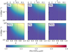 |
Fig. 3 Similar to Fig. 2, but now for the linear growth factors of the MG models. |
| In the text | |
|
Fig. 4 Comparison of the normalised linear growth factors (upper panel) and effective gravitational constant (lower panel) of the MG models, as labelled. The variations in these quantities are shown as a function of k for the redshift of the simulations, z = 0.5. |
| In the text | |
|
Fig. 5 Projected density field of DM and halos in a region of 1000×1000×20 h−3Mpc3 from seven different cosmologies at redshift z = 0.5. The upper panels display the DM density field and the lower panels the corresponding halo density field for the MG models, as labelled. These maps highlight the remarkable similarity in the density fields of MG and ΛCDM models. They also show that some models give rise to the formation of pronounced filaments, characterised by either a substantial thickness or a substantial length, as well as an increased prevalence of halos. |
| In the text | |
|
Fig. 6 Flowchart depicting the kernel and bias calibration using the COLA simulations as a reference to subsequently obtain the mapping bias relation, |
| In the text | |
|
Fig. 7 Comparison of the cross-power spectrum between the mock catalogues generated with BAM and their respective reference catalogues for the two calibrations: consistent-field calibration (solid line) and cross-field calibration (dashed line). The colours of the dashed lines have the same meaning as in the other plots. |
| In the text | |
|
Fig. 8 Projected density field in slices of 240 × 500 × 98 h−3 Mpc3 from a volume of 10003 h−3Mpc3 of the reference and mock catalogues for all cosmologies. Upper panels: Mocks from the consistent-field calibration. Bottom panels: Mocks from the cross-field calibration. Each sub-panel is divided in two; the left side corresponds to the reference halos from the N-body simulation and the right side to their respective mock obtained with BAM. The models are as labelled, and the colour bar indicates the density 1 + δh. Note that the ΛCDM model is a particular case in which the mock is the same in both the upper and lower panels, as it serves as the reference model. The circles in each panel display a region of interest where visual differences in overdensity are visible to the naked eye (dashed circle for reference halos and solid circle for mocks). |
| In the text | |
|
Fig. 9 Comparison of the PDFs (left), power spectra (P(k); middle), and reduced bispectra (Q(k1, k2, θ12); right) from the calibration stage obtained with BAM for the different MG models, as labelled. Upper panels: reference halo catalogues. Middle row: mock calibration created with BAM from the consistent MG DM field of each model. Lower row: mock calibration created with BAM from the DM field of the ΛCDM model. Note that all the comparisons are made between the MG model with respect to the ΛCDM field. |
| In the text | |
|
Fig. 10 Power spectrum and reduced bispectrum of the different MG mocks (dashed lines) compared to their respective reference catalogues (solid lines) for the studied calibrations, as labelled. Upper panels: consistent-field calibration, i.e. |
| In the text | |
Current usage metrics show cumulative count of Article Views (full-text article views including HTML views, PDF and ePub downloads, according to the available data) and Abstracts Views on Vision4Press platform.
Data correspond to usage on the plateform after 2015. The current usage metrics is available 48-96 hours after online publication and is updated daily on week days.
Initial download of the metrics may take a while.