| Issue |
A&A
Volume 690, October 2024
|
|
|---|---|---|
| Article Number | A141 | |
| Number of page(s) | 22 | |
| Section | Extragalactic astronomy | |
| DOI | https://doi.org/10.1051/0004-6361/202450162 | |
| Published online | 04 October 2024 | |
SUPER
VIII. Fast and furious at z ∼ 2: Obscured type-2 active nuclei host faster ionised winds than type-1 systems
1
Dipartimento di Fisica e Astronomia, Università di Firenze, Via G. Sansone 1, 50019 Sesto Fiorentino, Firenze, Italy
2
INAF - Osservatorio Astrofisico di Arcetri, Largo E. Fermi 5, 50125 Firenze, Italy
3
Max-Planck-Institut für Extraterrestrische Physik (MPE), Giessenbachstraße 1, D-85748 Garching, Germany
4
Centro de Astrobiología (CAB), CSIC–INTA, Cra. de Ajalvir Km. 4, 28850 – Torrejón de Ardoz Madrid, Spain
5
European Southern Observatory, Karl-Schwarzschild-Strasse 2, Garching bei München, Germany
6
Space Telescope Science Institute, 3700 San Martin Drive, Baltimore, MD 21218, USA
7
INAF – Osservatorio Astronomico di Padova, Vicolo dell’Osservatorio 5, I-35122 Padova, Italy
8
Dipartimento di Fisica e Astronomia “Augusto Righi”, Università di Bologna, Via P. Gobetti 93/2, 40129 Bologna, Italy
9
INAF – Osservatorio di Astrofisica e Scienza dello Spazio, Via Gobetti 93/3, 40129 Bologna, Italy
10
Dipartimento di Fisica, Università di Trieste, Sezione di Astronomia, Via G.B. Tiepolo 11, I-34131 Trieste, Italy
11
INAF – Osservatorio Astronomico di Trieste, Via G. Tiepolo 11, I-34143 Trieste, Italy
12
Scuola Normale Superiore, Piazza dei Cavalieri 7, I-56126 Pisa, Italy
13
Institute of Theoretical Astrophysics, University of Oslo, PO Box 1029 Blindern, 0315 Oslo, Norway
14
Department of Physics & Astronomy, University College London, Gower Street, London WC1E 6BT, UK
15
ESA, European Space Astronomy Centre (ESAC), Camino Bajo del Castillo s/n, 28692 Villanueva de la Cañada, Madrid, Spain
16
IFPU - Institute for fundamental physics of the Universe, Via Beirut 2, 34014 Trieste, Italy
17
School of Mathematics, Statistics and Physics, Newcastle University, Newcastle upon Tyne NE1 7RU, UK
18
School of Physics and Astronomy, Tel-Aviv University, Tel Aviv 69978, Israel
19
INAF – Osservatorio Astronomico di Roma, Via di Frascati 33, 00040 Monteporzio Catone, Rome, Italy
20
School of Physics and Astronomy, University of Southampton, Highfield, Southampton SO17 1BJ, UK
21
Kavli Institute for Cosmology, University of Cambridge, Madingley Road, Cambridge CB3 0HA, UK
22
Cavendish Laboratory - Astrophysics Group, University of Cambridge, 19 JJ Thompson Avenue, Cambridge CB3 0HE, UK
23
INAF – Istituto di Astrofisica Spaziale e Fisica Cosmica Milano, Via A. Corti 12, 20133 Milano, Italy
Received:
28
March
2024
Accepted:
3
July
2024
Abstract
We present spatially resolved VLT/SINFONI spectroscopy with adaptive optics of type-2 active galactic nuclei (AGN) from the SINFONI Survey for Unveiling the Physics and Effect of Radiative feedback (SUPER), which targeted X-ray bright (L2 − 10 keV ≳ 1042 erg s−1) AGN at cosmic noon (z ∼ 2). Our analysis of the rest-frame optical spectra unveils ionised outflows in all seven examined targets, as traced via [O III]λ5007 line emission, moving at v ≳ 600 km s−1. These outflows are clearly spatially resolved in six objects and extend on 2–4 kpc scales, but they are marginally resolved in the remaining one object. Interestingly, these SUPER type-2 AGN are all heavily obscured sources (NH ≳ 1023 cm−2) and host faster ionised outflows than their type-1 counterparts within the same range of bolometric luminosity (Lbol ∼ 1044.8 − 46.5 erg s−1). SUPER has hence provided observational evidence that the dichotomy of type-1 to type-2 at z ∼ 2 might not be driven simply by projection effects, but might reflect two distinct obscuring life stages of active galaxies, as predicted by evolutionary models. Within this picture, SUPER type-2 AGN might be undergoing the blow-out phase, where the large amount of obscuring material efficiently accelerates large-scale outflows via radiation pressure on dust, eventually unveiling the central active nucleus and signaling the start of the bright, unobscured type-1 AGN phase. Moreover, the velocities of the overall population of ionised outflows detected in SUPER are comparable with the escape speed of their dark matter haloes, and they are in general high enough to reach distances of 30–50 kpc from the centre. These outflows are hence likely to sweep away the gas (at least) out of the baryonic disk and/or to heat the host gas reservoir, thus reducing and possibly quenching star formation.
Key words: techniques: imaging spectroscopy / galaxies: active / galaxies: evolution / galaxies: high-redshift / quasars: emission lines
Corresponding author; This email address is being protected from spambots. You need JavaScript enabled to view it.
© The Authors 2024
 Open Access article, published by EDP Sciences, under the terms of the Creative Commons Attribution License (https://creativecommons.org/licenses/by/4.0), which permits unrestricted use, distribution, and reproduction in any medium, provided the original work is properly cited.
This article is published in open access under the Subscribe-to-Open model.
Open access funding provided by Max Planck Society.
1. Introduction
A key question in galaxy evolution is how active galactic nuclei (AGN) interact with their host galaxy and shape its physical properties, from gas content to star formation (SF) and chemical enrichment. This so-called AGN feedback typically acts via massive outflows (e.g. King 2005; Fabian 2012; Costa et al. 2014), that are powered on sub-parsec scales by the radiative output of accreting supermassive black holes (BH), and are then accelerated up to galaxy scales of ∼1–10 kpc (e.g. King & Pounds 2015). These winds are considered the main cause for quenching SF within their host by heating or expelling the gas reservoir from which new stars form (i.e. preventive versus ejective feedback), and settling the observed scaling relations between BH mass and host galaxy properties (e.g. Ferrarese & Merritt 2000; Marconi & Hunt 2003; Kormendy & Ho 2013; Marasco et al. 2021).
To date, we have much observational evidence of AGN-driven outflows from low (e.g. Feruglio et al. 2010; Harrison et al. 2014; Woo et al. 2016) to high redshift (z > 1; e.g. Maiolino et al. 2012; Förster Schreiber et al. 2014; Carniani et al. 2024) in different gas phases (e.g. Cicone et al. 2018). While millimeter to sub-millimeter interferometric observations are optimally suited for investigating the cold molecular (T < 100 K) component of AGN-driven outflows (typically via CO line emission; Cicone et al. 2014; Morganti et al. 2015; Chartas et al. 2020), optical/near-IR integral field spectroscopy (IFS) enables detailed spatially resolved studies of the warmer ionised outflow component. To trace ionised outflows, the most commonly adopted tracer is the optical [O III]λ5007 line emission (e.g. Cano-Díaz et al. 2012; Venturi et al. 2018; Marshall et al. 2023). This forbidden line transition can only originate in low-density regions (ne < 106 cm−3), and any potential contamination from a high-density AGN broad-line region (BLR) is accordingly excluded. Therefore, [O III]λ5007 is an excellent tracer of ionised gas that is extended on scales of 1–10 kpc.
Based on high-quality IFS observations that were obtained with ground-based adaptive optics (AO) assisted facilities or from space with the James Webb Space Telescope, AGN-driven ionised outflows and feedback mechanisms have been deeply investigated at z > 1 (e.g. Förster Schreiber et al. 2014; Perna et al. 2015a, 2023; Wylezalek et al. 2022; Cresci et al. 2023; Marshall et al. 2023; Vayner et al. 2023), with the primary focus on the so-called cosmic noon (z ∼ 2), where the SF and BH accretion histories both reach the peak of their activity (Madau & Dickinson 2014). This makes the redshift range z ∼ 1–3 the golden epoch of AGN feedback, in which its effects are expected to be maximised.
Nonetheless, the high-redshift search has primarily focused on brighter distant sources so far (Lbol > 1046 erg s−1; e.g. Bischetti et al. 2017; Perrotta et al. 2019), which are easier to detect and examine. This has led to a biased census of high-redshift AGN-driven outflows. In addition to this, the lack of direct observational evidence that would confirm (or disprove) key theoretical predictions prevents us from a clear and complete picture of AGN feedback and outflows. Several questions are still open, for instance, how AGN-driven outflows really affect their host galaxy, whether they quench SF activity efficiently, or whether they are representative of a particular life stage of the evolution of the galaxies.
One of these theoretical scenarios that still waits for observational proof predicts that AGN galaxies experience a first dust-enshrouded life stage (e.g. Hopkins et al. 2006; Menci et al. 2008), in which the central nucleus is obscured by dust and gas that fuel supermassive BH growth and SF efficiently. This sets the stage for the short-lived (a few million years) blow-out phase (e.g. Hopkins et al. 2008), during which powerful AGN-driven winds sweep away obscuring material and cause the central AGN to become visible and unobscured. This evolutionary scenario was proposed to explain the observed dichotomy between red and blue quasars (e.g. Brusa et al. 2010; Klindt et al. 2019; Perrotta et al. 2019; Fawcett et al. 2023), the former representing the brief obscured transitional phase featured by powerful winds that are accelerated via radiation pressure on dust (e.g. King & Pounds 2015; Costa et al. 2018). For this reason, X-ray bright (easier to detect) but optically obscured AGN at z = 1 − 3 have been deeply investigated for years as optimal candidates undergoing the blow-out phase (e.g. Brusa et al. 2015, 2016; Cresci et al. 2015, 2023; Perna et al. 2015a,b; Veilleux et al. 2023). They were hence considered the most promising targets for catching AGN feedback and outflows in action.
To draw a coherent picture of AGN feedback at cosmic noon, it is fundamental to conduct systematic and unbiased searches for outflows in statistically large samples. The KMOS1 AGN Survey at High redshift (KASHz; Harrison et al. 2016) has provided spatially resolved information for hundreds of X-ray selected AGN, revealing ionised gas velocities that are likely indicative of outflows in about 50% of the examined sample (Harrison et al. 2016). However, KASHz employed seeing-limited observations with a typical spatial resolution of 4–9 kpc at z > 1 (i.e. > 0.5″), which is not sufficient to trace outflows and their properties in detail. To reach higher spatial resolution, we can exploit more time-consuming AO-assisted observations of smaller samples that are still representative of the AGN population at z ∼ 2.
Our completed Large Programme Survey for Unveiling the Physics and Effect of Radiative feedback (SUPER; PI: V. Mainieri, ID: 196.A-0377), carried out with the Spectrograph for INtegral Field Observations in the Near Infrared (SINFONI; Eisenhauer et al. 2003) at the Very Large Telescope (VLT) of the European Southern Observatory (ESO), has collected AO-assisted IFS data of a representative sample of X-ray AGN (L2 − 10 keV ≳ 1042 erg s−1) at z ∼ 2, spanning a wide range of bolometric luminosity (Lbol = 1044 − 48 erg s−1). Presented by Circosta et al. (2018), the SUPER survey offers us the extraordinary possibility of investigating AGN-driven ionised outflows in a few dozen AGN at cosmic noon that are selected in an unbiased way with respect to the chance of hosting outflows. With the SINFONI AO system, we reached exquisite angular resolutions of 0.2″–0.5″ that can probe spatial scales down to 2–4 kpc at z ∼ 2.
In this perspective, this paper continues the series of publications dedicated to SUPER2 by presenting SINFONI observations of the type-2 AGN subsample. In particular, this work complements the analysis carried out by Kakkad et al. (2020) of the ionised outflows in the SUPER type-1 AGN (see also Vietri et al. 2020) by extending the study of ionised outflows to the SUPER type-2 systems (see also Lamperti et al. 2021). We still employ [O III]λ5007 line emission to trace large-scale ionised outflows and then compare the inferred properties of the type-2 ionised outflows with those of the type-1 counterparts with the aim to uncover possible differences between these two AGN populations.
This paper is organised as follows. In Sect. 2, we introduce the SUPER type-2 AGN subsample examined in this work and present our SINFONI observations as well as the data reduction strategy. In Sect. 3, we describe the fitting procedure we adopted to derive ionised gas properties from SINFONI data. The inferred results on ionised outflows are then presented in Sect. 4, and in Sect. 5, they are studied as a function of host galaxy properties and compared with those previously obtained for the SUPER type-1 AGN (Kakkad et al. 2020). A further discussion of our main findings as well as a comparison with results from the literature is found in Sect. 6. We finally draw our conclusions in Sect. 7. A ΛCDM flat cosmology with Ωm, 0 = 0.3, ΩΛ, 0 = 0.7, and H0 = 70 km s−1 Mpc−1 is adopted throughout this work.
2. Sample and data description
The sample presented in this work is part of the SUPER survey (ID: 196.A-0377; PI: V. Mainieri), which acquired near-IR IFS observations of 333 blindly selected X-ray AGN at z ∼ 2 (see Circosta et al. 2018 for details of the sample selection and properties). The total 33-AGN observed sample consists of 21 type-1 AGN that were investigated in detail by Kakkad et al. (2020, 2023), and 12 type-2 AGN, whose SINFONI observations are presented and analysed in this work. These three papers investigate ionised outflows with an unprecedented spatial resolution of about the kiloparsec scale in an unbiased sample of AGN at cosmic noon, using [O III] line emission as outflow tracer, and search for links between outflow properties (e.g. velocity or mass rate) and fundamental AGN and/or host galaxy parameters (e.g. bolometric luminosity, stellar mass, and star formation rate). In the following subsections, we first introduce the observed type-2 AGN subsample (Sect. 2.1), and then we briefly describe the observations, the data reduction, and the final type-2 AGN sample (i.e. seven objects) analysed in this paper (Sect. 2.2).
2.1. Observed SUPER type-2 AGN subsample
SUPER targeted 12 type-2 AGN in total: six sources are from the Chandra Deep Field-South (CDF-S; Luo et al. 2017); and the other six are from the COSMOS-Legacy survey (Civano et al. 2016). Before they were observed with SINFONI, they were identified as type-2 systems based on the absence of BLR emission in the archival rest-frame UV spectra (Circosta et al. 2018). Their type-2 spectral classification was then confirmed by SINFONI observations, showing no BLR components in rest-frame optical Balmer hydrogen lines (Hα and Hβ), which are typically less extincted than UV emission lines. In Table 1, we list some of the main properties of the 12 observed type-2 AGN, including spectroscopic redshift z; bolometric luminosity Lbol, stellar mass M*, and SFR, all derived from a spectral energy distribution (SED) fitting (Circosta et al. 2018); 2–10 keV X-ray luminosity L2 − 10 keV and the hydrogen column density NH inferred from archival X-ray spectra (Circosta et al. 2018). The redshift values were obtained from rest-frame optical SINFONI spectra (see Sect. 3.1), except for sources that were undetected or marginally detected (five in total) in our SINFONI data (see Sect. 2.2). For these sources, the redshift was measured from archival rest-frame UV spectra (marked with the dagger). Depending on the quality of the [O III] detection in SINFONI H-band spectra, the last column shows the objects that are included in the final type-2 AGN sample (i.e. seven objects), which are analysed in this work (details in Sect. 2.2).
Main properties of the 12 observed type-2 AGN from SUPER.
2.2. Observations and data reduction
SUPER targets were observed with SINFONI between November 2015 and December 2018. All observations were planned to be carried out in AO mode using a laser guide star (LGS), covering the H band, targeting the Hβ and [O III]λλ4959,5007 emission lines, and the K band, targeting Hα, [N II]λλ6549,83, and [S II]λλ6716,31.
Due to the absence of suitable stars close to the targets, observations of 10 out of 12 type-2 AGN were performed in AO-assisted mode without a tip-tilt star (i.e. in seeing-enhancer mode; Davies et al. 2008), using both H and K gratings (R ∼ 3000 and R ∼ 4000, respectively); the remaining 2 objects were observed with no-AO (cid_1253 with H and K gratings; cid_971 with the HK grating, R ∼ 1500) in order to optimize the time available during the visitor-mode observing run, which was reduced because of bad weather conditions. For AO-assisted observations, we adopted a plate scale of 3″ × 3″ with a spatial sampling of 0.05″ × 0.1″, then re-sampled to 0.05″ × 0.05″ in the final datacube. For the 2 targets observed in seeing-limited mode, we instead selected the largest field of view (FoV; 8″ × 8″), corresponding to a pixel scale of 0.25″ × 0.25″. Before or after each observing block, a dedicated bright star was observed to estimate the point spread function (PSF) of our AO-assisted SINFONI observations as the full width at half maximum (FWHM) of a 2D Gaussian fitting to the total flux distribution of the PSF star (θPSF values in Table 2).
SINFONI observations of the 12 SUPER type-2 AGN.
We summarise the main steps of the reduction procedure applied to SINFONI type-2 AGN datacubes below, and we refer to Kakkad et al. (2020) for a detailed description of the SUPER observational strategy. We reduced all observations using the ESOREX pipeline (3.1.1), which returns a distortion-corrected and wavelength-calibrated datacube of the science target, as well as of the PSF and telluric stars. We then removed background sky emission via the IDL routine skysub.pro (Davies 2007), and used our own custom-made python routines to perform flux calibration (based on Piqueras López et al. 2012) and to reconstruct the final datacube for each observed target. As a final check, we compared the synthetic photometry measured from SINFONI-integrated spectra with archival photometric measurements (Circosta et al. 2018) and the synthetic photometry from KMOS-integrated spectra, when available (Scholtz et al., in prep.). From this comparison, we estimated a typical relative uncertainty on the flux calibration of our SINFONI data of about 20% for all employed bands.
In Table 2, we show the main parameters of SINFONI observations of the 12 SUPER type-2 AGN. For each target, we specify the observing mode (AO/noAO), and list the following parameters for the corresponding adopted grating (H, K, HK): The absolute (AB) magnitude measured from SINFONI-integrated spectra, total exposure time texp, spatial resolution θPSF (i.e. PSF FWHM), and detected emission lines for the seven objects with [O III] detected with a total, spatially integrated S/N > 2, which is the crucial tracer of ionised outflows employed in our study. Five of these systems also have Hα+[N II] detected with an S/N > 2, but Hα is entirely undetected or marginally detected (S/N < 2) in cid_1057 and cid_1143, respectively. Although not suitable for our analysis, we report for completeness that we also marginally detected [O III] and/or Hα in XID427 and cid_1253. Finally, the remaining three targets (i.e. XID522, XID57 and cid_971) are entirely undetected in SINFONI observations. We point out that these non-detections or poor detections are a consequence of the short integration time. Observing time was lost because of bad weather conditions, which particularly penalised SUPER type-2 objects, which are also the faintest sources of the SUPER sample (Lbol < 1046 erg s−1).
In the following, we focus on the seven type-2 AGN with [O III] detected at S/N > 2, which allows us to perform a spatially resolved analysis of [O III] line emission and thus search for ionised outflow signatures. These sources all have a ‘yes’ in the last column of Table 1. In particular, three of them are CDF-S sources (XID36, XID419, and XID614), and four are from COSMOS (cid_1057, cid_1143, cid_2682, and cid_451).
3. Data analysis
In this section, we analyse SINFONI H-band observations of the seven well-detected type-2 AGN (S/N > 2) in [O III] to spatially map the [O III] line emission and its kinematics in a search for evidence of high-velocity outflowing gas (Sect. 3.1). Unfortunately, the quality of the K-band data is worse (i.e. lower S/N) for most objects, which prevents us from an accurate mapping of the K-band line emission across the SINFONI FoV. In Sect. 3.2 we use combined integrated measurements of Hα and Hβ fluxes from K- and H-band data, respectively, to estimate dust extinction. Because these targets are obscured (type-2) AGN, it is crucial to correct for dust extinction to obtain reliable estimates of the outflow energetics (see Sect. 4.2).
3.1. Spectral fitting
For the spectral fitting of SINFONI H-band datacubes, we adopted the fitting code presented in Marasco et al. (2020) (see also Tozzi et al. 2021 for more details), and fitted all cubes in the rest-frame optical wavelength range of 4800–5200 Å. Because they are distant type-2 AGN, their SINFONI spectra show neither BLR emission nor a strong (AGN and/or stellar) continuum, but consist of only narrow (FWHM ≲ 2000 km s−1) emission lines that either originate from an AGN narrow line region (NLR) or are due to a different kinematics (i.e. an outflow or disk rotation). In addition to the [O III]λλ5007,4959 emission line doublet (which was detected in all seven examined sources), we also detected faint Hβ line emission in four H-band datacubes (i.e. XID36, XID914, cid_1143, and cid_1057; see Figs. 1–3).
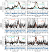 |
Fig. 1. Integrated H- and K-band spectra extracted from SINFONI datacubes of XID36 (top), XID419 (middle), and XID614 (bottom), with a radius aperture of 0.25″, after subtracting continuum emission that was modelled with a first-degree polynomial. The data are shown in black, and the total emission-line model is overplotted in red. For multi-Gaussian modellings, we separately plot the narrow systemic (light blue) and broad high-velocity components (green) that are associated with outflows. In the top right panel, the solid and dashed green lines represent the outflow component of Hα and [N II] doublet, respectively. The mean velocity v and the velocity dispersion σ values of each Gaussian component are displayed. The shaded grey regions indicate masked channels that are contaminated by sky line residuals, and the vertical dotted lines mark the rest-frame emission line wavelengths at the redshift of each source, as computed in Sect. 3.1. Below each main panel, a second panel shows the corresponding residuals (i.e. data–model). |
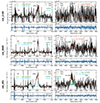 |
Fig. 2. Integrated H- and K-band spectra extracted from SINFONI datacubes of cid_1143 (top), cid_2682 (middle), and cid_451 (bottom), with a radius aperture of 0.25″, after subtracting continuum emission that was modelled with a first-degree polynomial. Same as in Fig. 2. In the K-band spectrum of cid_1143, we fit only the Hα line emission due to the low S/N (S/N < 2) of this dataset. |
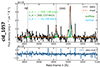 |
Fig. 3. Integrated H-band spectrum of cid_1057, extracted from a SINFONI datacube with a radius aperture of 0.25″, after subtracting continuum emission that was modelled with a first-degree polynomial. Same as in Fig. 2. Three Gaussian components are used to properly model the [O III] line profile: One component was used for the systemic narrow line emission (light blue), and two components were used for the blue and red wings detected in [O III] (different greens). |
As a first step, we applied a spatial Gaussian smoothing of the data channel by channel to enhance the visibility of real gas structures. To do this without deteriorating the instrumental PSF, we smoothed each datacube with a Gaussian kernel with a width of σsmooth ∼ 0.1 − 0.2″, that is, as large as possible, but still smaller than the instrumental PSF FWHM (i.e. σsmooth < θPSF/2.35). After this, we modelled the observed line emission spaxel by spaxel via multiple Gaussian components, following the prescriptions summarised below:
-
We fitted the [O III]λλ5007,4959 line doublet with two Gaussian components with the same kinematics (mean velocity v and velocity dispersion σ), imposing a fixed flux ratio of 3. Hereafter, we refer to the brighter doublet component (i.e. [O III]λ5007) as [O III].
-
When detected, faint Hβ line emission was modelled with v and σ fixed to the best-fit values obtained for [O III], that is, with flux as the only free parameter.
-
In each spaxel, we reiterated the line modelling using an increasing number of Gaussian components for each emission line, from one to the maximum number that best reproduces complex line profiles in high S/N spaxels. We then selected the optimal (minimum) number of Gaussian components required in each spaxel via a Kolmogorov–Smirnov test on the residuals. Five H-band datasets required up to two Gaussian components; cid_1057 required up to three components, given the detected blue and red [O III] wings. One component was instead sufficient to model single-spaxel line emission in XID419.
-
We also added a first-degree polynomial to reproduce any faint continuum emission over the entire fitted wavelength range.
Several spectra required multiple Gaussian components to simultaneously reproduce the narrow low-velocity line emission and broad high-velocity wings in the [O III] line profile. Whereas the latter are considered the typical signature of fast-outflowing gas (discussed in Sect. 4.1), narrow low-velocity line emission is typically due to nearly systemic gas motions (e.g. NLR or disk rotation). We used the narrowest [O III] line component to measure the redshift of each source: We extracted an H-band integrated spectrum from a small aperture (0.1″ radius) centred on the overall H-band emission peak (corresponding to the [O III] emission peak), and set the peak of the narrowest [O, III] line component to 0 km s−1. We estimate an uncertainty of Δz = 0.001 on our [O III] based measurements of z because of the SINFONI H-band spectral resolution (R ∼ 3000) and the typical S/N of the line.
3.2. Dust extinction from integrated spectra
Since the targets examined in this work are all type-2 AGN that are highly obscured in the X-rays (NH ≳ 1023 cm−2; Circosta et al. 2018), the rest-frame optical emission is expected to be significantly affected by extinction effects. In particular, in Sect. 4.2 we correct our measurements of the [O III] outflow luminosity for dust extinction to estimate the intrinsic energetics of ionised outflows. Below, we derive the rest-frame optical dust extinction from spatially integrated Hα/Hβ ratios for the seven type-2 AGN.
To accurately correct for dust extinction, we should in principle (i) account for spatial variations in the Hα/Hβ ratios across the FoV using spaxel-by-spaxel measurements and (ii) consider extinction effects exclusively on the outflow component, which may differ from those affecting the bulk of the ionised gas or any other kinematic component (e.g. disk rotation or AGN NLR). The S/N on Hα and Hβ in our SINFONI data is not high enough for such an accurate spatial mapping of dust extinction, however. Their detection is mostly limited to central brighter spaxels, and Hβ is undetected in three sources (even in the integrated spectra), whereas Hα is entirely undetected in cid_1057 and only marginally (S/N < 2) detected in cid_1143. Therefore, we extracted integrated K- and H-band spectra of each object to increase the S/N on Hα and Hβ to estimate (or place constraints on) the dust extinction. The only target of the seven-AGN sample for which this is not possible is cid_1057, which is entirely undetected in Hα. In the following, we therefore describe first how we estimated (or constrained) the dust extinction from SINFONI-integrated spectra in the six objects in which Hα was detected, and then we describe the assumptions we adopted for cid_1057.
We extracted integrated K- and H-band spectra of each target using an aperture with a radius of ∼0.25″ centred on the source (Figs. 1, 2, 3), and we fitted them following the prescriptions described in Sect. 3.1. In particular, Gaussian profiles fitted to Hα and [N II]λλ6549,83 were constrained to have the same velocity and velocity dispersion, with the additional constraint of a fixed flux ratio of 3 on the two [N II] doublet components. In XID36, we also modelled faint [S II]λλ6716,31 line emission following the prescriptions adopted for Hβ in the H-band datasets. In most cases, one Gaussian component was enough to reproduce the K-band emission lines; XID36 and cid_451 instead required an additional broader component (σ ∼ 700 km s−1 in XID36, and σ ∼ 400 km s−1 in cid_451).
In Figs. 1 and 2, we show the H- and K-band spectra that were extracted with a radius aperture of 0.25″ from SINFONI datacubes after subtracting the first-degree polynomial that was used to reproduce any faint residual continuum emission. Over the data we plot the total emission-line model and, for multi-Gaussian fittings, single components used to reproduce narrow, systemic line emission, and broad high-velocity line emission, likely associated with ionised outflows. In Fig. 3, we also show an integrated H-band spectrum of cid_1057 that was extracted with the same radius aperture of 0.25″. In this source, the [O III] emission line exhibits an asymmetric profile that is well reproduced by three Gaussian components: one for systemic, narrow line emission (light blue), two for the blue and red [O III] wings (different greens). Excluding XID419, the only target requiring a single-Gaussian modelling, we find mean values of ⟨|v|⟩ ∼ 380 km s−1 and ⟨σ⟩∼440 km s−1 for the broad outflow (green) component and ⟨|v|⟩ ∼ 20 km s−1 and ⟨σ⟩∼160 km s−1 for the narrow nearly systemic component.
Because we detected no broad high-velocity wings in the Hβ line profile (which might be associated with outflows) in any object (in Hα only in XID36 and cid_451), we took the integrated total Hα/Hβ ratios to obtain an estimate of the total dust extinction (Calzetti et al. 2000) and assumed that it also affects the outflow emission. For XID36, XID614, and cid_1143, for which both hydrogen lines were detected, we estimated AV and the relative uncertainty via an error propagation. Because the S/N is low on Hα and Hβ, we obtain a value of AV for cid_1143 that is consistent with 0 (i.e. no extinction) within the uncertainty (AV = 1.2 ± 1.8). Because AV must be non-negative, we adopted  . In XID419, cid_2682, and cid_451, where we do not detect Hβ, we instead estimated a lower limit to AV, considering a 2σnoise upper limit to the Hβ flux. Finally, for cid_1057, the only source that is entirely undetected in Hα, we considered an AV value that was computed as the average of the three AV measurements obtained for XID36, XID614, and cid_1143, taking the maximum distance of these estimates from the mean as the uncertainty (i.e. AV = 1.8 ± 1.0). We use these AV values in Sect. 4.2 to obtain the dust-corrected [O III] outflow flux in each source, and hence, the corresponding outflow mass.
4. Results
4.1. Evidence of spatially resolved outflows
Our spectral modelling of the [O III] line emission has clearly revealed prominent wings in the [O III] line profile of four galaxies (i.e. XID36, cid_1143, cid_451, and cid_1057; see Figs. 1–3). This indicates gas that moves at high speed with respect to the galaxy systemic velocity. In XID614 and cid_2682, the [O III] line profile also shows a faint blue wing (see Figs. 1 and 2), but any possible blue [O III] wing in XID419 is hard to assess at first glance (see Fig. 1) because the residual sky emission is so bright. In this section, we inspect the kinematic maps of the [O III] line emission (Figs. 4–7) to confirm the presence of ionised outflows in detections with a higher S/N and to search for evidence in more ambiguous cases.
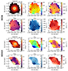 |
Fig. 4. Morphology and kinematics of ionised gas in XID36 and XID419 as traced by the total [O III] line emission. For each target, the maps show the intensity (moment-0) field; the v50, v10, and v90 percentile velocities and the w80 line width; and the ratio f300 of the flux contained in [O III] wings (i.e. |v|> 300 km s−1) to the moment-0 flux. The dashed and dotted circles correspond to the radius aperture of 0.25″ we used to extract the integrated spectra (Sect. 3.2) and to the mean H-band PSF with a radius of ⟨θPSF⟩/2, respectively (see Table 2). The two circles have the same 0.25″ radius in XID419. In all maps, we apply an S/N > 3 cut and mark the position of the [O III] peak emission with a cross. |
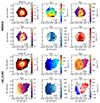 |
Fig. 5. Morphology and kinematics of ionised gas in XID614 and cid_1143 as traced by the total [O III] line emission. Same as in Fig. 4. |
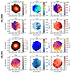 |
Fig. 6. Morphology and kinematics of ionised gas in cid_2682 and cid_451 as traced by the total [O III] line emission. Same as in Fig. 4. |
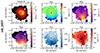 |
Fig. 7. Morphology and kinematics of ionised gas in cid_1057 as traced by the total [O III] line emission. Same as in Fig. 4. |
In Figs. 4–7, we show maps of the [O III] line emission with a cut at S/N > 3. The maps display the spatial distribution and kinematics of ionised gas in all seven type-2 AGN. The maps in the first column show the [O III] intensity field computed as the moment-0 of the total line profile (upper panel); and ratio values (f300; lower panel) of the flux in high-velocity channels (|v|> 300 km s−1) to the moment-0 flux, which is a simplified but reasonable approximation of the [O III] flux that is carried by outflows (Kakkad et al. 2020). For the seven type-2 AGN, we find that the total (i.e. spatially integrated) flux at |v|> 300 km s−1 represents a significant fraction of the total moment-0 flux. It ranges from 21% (in cid_1057) to 66% (in XID36).
In addition, the maps in the second and third columns of Figs. 4–7 display the ionised gas kinematics described in terms of non-parametric percentile velocities4. Compared to the parametric values, the percentile velocities have the advantage of being independent of the adopted fitting function (e.g. the number of Gaussian components), which in turn may strongly depend on the S/N of the examined data (e.g. Harrison et al. 2014; Zakamska & Greene 2014). In particular, we computed the v50, v10, and v90 velocities and the w80 line width (i.e. w80 = v90 − v10), which is approximately equal to the FWHM of a Gaussian profile. Extreme v10 and v90 values are widely adopted as a reliable approximation of the outflow velocity for its approaching and receding components (e.g. Harrison et al. 2014; Carniani et al. 2015; Cresci et al. 2015), respectively. Compared to the moment-1 and moment-2 values (i.e. mean velocity and velocity dispersion, respectively), which may be affected by significant geometrical projection effects, v10 and v90 help us to avoid possible underestimates of the real outflow velocity because the intrinsic outflow geometry and inclination to the line of sight are not known. The maps of v10 and v90 feature high velocities overall, with absolute values up to 800–1100 km s−1 in four targets (XID36, XID419, cid_1143, and cid_451), and values up to 600–700 km s−1 in the remaining three (XID614, cid_1057, and cid_2682). These high velocities are accompanied by w80 line widths larger than 800 km s−1 in most of the FoV of all targets, and the highest values are 1000 km s−1 at least (about 1700 km s−1 in XID36 and 1200 km s−1 in cid_451).
Ionised outflows are the most likely explanation for the high-velocity kinematics that is observed in all targets because alternative phenomena can hardly lead to such high values of the velocity and line width. SF-driven outflows are typically characterised by lower velocities (e.g. Arribas et al. 2014; Förster Schreiber et al. 2019), and galactic inflows are mostly observed in absorption with low bulk velocities and σ values (e.g. Bouché et al. 2013). Large line widths might also be due to turbulence in the interstellar medium induced by the interaction of nuclear activity with the host environment, as observed in low-redshift type-2 active galaxies (e.g. Woo et al. 2016; Fischer et al. 2018; Venturi et al. 2021; Girdhar et al. 2022). These turbulence-induced effects are often associated with relatively low centroid velocities (i.e. |v|< 200 − 300 km s−1), however, which are typical of gas at systemic or following rotation (Woo et al. 2016; Fischer et al. 2018). This does not seem to be the case of the broad components that reproduce the [O III] line wings in the SUPER type-2 systems, which exhibit centroid velocities |v|≳300 km s−1 (see the green v values shown in Figs. 1–3), which are probably not associated with galaxy rotation. Moreover, we point out that turbulence-induced effects have been traced so far in observations of local Seyfert galaxies at high spatial resolution and sensitivity (see e.g. Fischer et al. 2018; Venturi et al. 2021; Girdhar et al. 2022). As a consequence, it might be hard to detect them in lower-quality observations at z ∼ 2 such as SUPER, with a spatial resolution of 2–4 kpc.
Similarly, the observed large [O III] line widths and prominent asymmetries (mostly blueshifted wings) can hardly be accounted for by merging scenarios. This is also supported by the lack of clear [O III] double peaks and by the relatively unperturbed morphology of the stellar continuum emission as traced by rest-frame 260 μm FIR continuum emission (when available for SUPER targets; see Lamperti et al. 2021). Although it is harder to detect than line emission due to gas, the stellar continuum can reveal a second merging galaxy better. The only SUPER galaxy showing some degree of perturbed morphology is cid_1143, which exhibits an offset of about 2 kpc between the centroids of the rest-frame optical line emission (i.e. Hα and [O III]) and the rest-frame 260 μm FIR continuum (Lamperti et al. 2021). This may indicate the presence of a companion for this galaxy, but, even if this were the case, this is not expected to contribute to the flux in the galaxy center given the offset of the possible companion from FIR continuum. The centre has v10 velocities of about 1000 km s−1. For the other sources, we can instead likely rule out early mergers based on the observational evidence available so far, although the S/N of our SINFONI observations might not be sufficient to detect faint merger signatures and to identify final-state mergers in particular.
Unlike v10 and v90, v50 velocities are useful to describe the velocity field of the component that dominates the overall kinematics of ionised gas. In all galaxies, we find moderate v50 values (|v50|< 400 km s−1; even |v50|< 100 km s−1 in XID614 and cid_2682), with a predominance of blueshifted v50 values. This means that a significant fraction of [O III] line emission is found in the blue line wing, which further supports that fast ionised outflows are present in these galaxies. In XID36 instead, the v50 velocities appear redshifted almost everywhere (reaching 400 km s−1) as a consequence of the extended [O III] red wing, which dominates the overall [O III] kinematics in this object (see Fig. 1). In a few galaxies, we also detect a smooth velocity gradient of v50: in cid_1143 it is outflow-dominated, with all blueshifted v50 velocities with an increasing absolute value from NW to SE (N is up, E to the left). In contrast, in XID419 and XID614, the outflow emission does not seem to be the dominant component. The v50 field is consistent with disk rotation, with velocities ranging from negative to positive values passing through the galaxy centre. The presence of outflows in these two galaxies is better highlighted by the high values of v10 and v90, as discussed previously.
In all maps of Figs. 4–7, the two circles correspond to the aperture used in Sect. 3.2 to extract integrated SINFONI spectra (dashed); and to the mean H-band PSF (dotted), that is, to an aperture with a radius equal to ⟨θPSF⟩/2 (see Table 2). In XID419 (Fig. 4), the two circles have the same radius. Compared to the corresponding H-band PSF, the extent of the S/N > 3 [O III] line emission at |v|> 300 km s−1 is clearly larger than the instrumental PSF radius in all galaxies except XID614. This ensures that the high-velocity [O III] emission associated with the outflows is spatially resolved in at least six objects of our sample. In XID614, the S/N > 3 [O III] maps and H-band PSF have approximately the same extent in all directions (see Fig. 5). That structures and variations in gas kinematics are visible across the FoV of XID614 suggests, however, that the high-velocity [O III] line emission at a large distance is at least marginally spatially resolved in our data.
4.2. Ionised outflow properties and energetics
Because Hβ is detected at low S/N in our H-band observations as a result of extinction effects, we derived the ionised outflow properties from the higher-S/N [O III] line emission5. Properties such as the outflow velocity vout, the radial extent Rout, and the [O III] luminosity ![Mathematical equation: $ L^{\mathrm{[OIII]}}_{\mathrm{out}} $](/articles/aa/full_html/2024/10/aa50162-24/aa50162-24-eq23.gif) can be directly measured from SINFONI data, while other physical quantities (i.e. the electron density ne and the oxygen abundance [O/H]) must be assumed in the calculation of outflow mass rate Ṁout.
can be directly measured from SINFONI data, while other physical quantities (i.e. the electron density ne and the oxygen abundance [O/H]) must be assumed in the calculation of outflow mass rate Ṁout.
4.2.1. Directly measured outflow properties
The outflow properties that can be measured directly are vout, Rout, and ![Mathematical equation: $ L^{\mathrm{[OIII]}}_{\mathrm{out}} $](/articles/aa/full_html/2024/10/aa50162-24/aa50162-24-eq24.gif) . As the outflow velocity vout, we considered the maximum absolute value of all observed v10 or v90 velocities for each target (i.e. vout = max[|v10|,|v90|]). This definition is widely adopted in the literature (e.g. Cresci et al. 2015; Carniani et al. 2015; Tozzi et al. 2021; Vayner et al. 2021a,b) and relies on the assumption that all observed lower velocities are a consequence of projection effects. Other works instead used w80 as the outflow velocity (e.g. Harrison et al. 2012; Kakkad et al. 2016, 2020) because w80 is less affected by projection effects than v10 and v90. We point out, however, that the w80 values depend more strongly on the line shapes and systematically lead to higher velocities for symmetric line profiles than for asymmetric ones, where only one wing is detected as a possible consequence of dust extinction. Dust effects indeed seem to be the most likely explanation for the (blueshifted) asymmetric [O III] profiles found in most of our type-2 AGN, which can hardly be accounted for by standard unified models (e.g. Antonucci 1993; Urry & Padovani 1995; further discussions are presented in Sect. 6).
. As the outflow velocity vout, we considered the maximum absolute value of all observed v10 or v90 velocities for each target (i.e. vout = max[|v10|,|v90|]). This definition is widely adopted in the literature (e.g. Cresci et al. 2015; Carniani et al. 2015; Tozzi et al. 2021; Vayner et al. 2021a,b) and relies on the assumption that all observed lower velocities are a consequence of projection effects. Other works instead used w80 as the outflow velocity (e.g. Harrison et al. 2012; Kakkad et al. 2016, 2020) because w80 is less affected by projection effects than v10 and v90. We point out, however, that the w80 values depend more strongly on the line shapes and systematically lead to higher velocities for symmetric line profiles than for asymmetric ones, where only one wing is detected as a possible consequence of dust extinction. Dust effects indeed seem to be the most likely explanation for the (blueshifted) asymmetric [O III] profiles found in most of our type-2 AGN, which can hardly be accounted for by standard unified models (e.g. Antonucci 1993; Urry & Padovani 1995; further discussions are presented in Sect. 6).
We therefore adopted vout = max[|v10|,|v90|] to define the outflow velocity, unlike the previous w80-based approach adopted in Kakkad et al. (2020) for the SUPER type-1 sample. However, as pointed out in Sect. 4.1, all type-2 AGN show w80 > 800 km s−1 in most of the FoV, and they therefore meet the w80 > 600 km s−1 criterion used in Kakkad et al. (2020) to identify the [O III] outflow emission (e.g. see also Harrison et al. 2016).
Overall, we find wind velocities within the range vout ∼ 600 − 1100 km s−1, with a mean outflow velocity ⟨vout⟩∼830 km s−1. For comparison, we also computed the outflow velocity for each object using another definition widely adopted in literature, that is vmax = vbro + 2σbro (Rupke & Veilleux 2013), where vbro and σbro are the velocity and velocity dispersion, respectively, of the broad Gaussian components associated with the outflows. This parametric definition of the outflow velocity typically delivers values that are slightly higher than the vout definition based on v10, 90, but because they were adopted in several works (e.g. Brusa et al. 2015; Fiore et al. 2017; Leung et al. 2019; Perrotta et al. 2019; Kakkad et al. 2020), it is a useful quantity to compute for a comparison of our results with results from the literature (see Sect. 6). For XID419, we estimate vmax as twice the σ value of the single Gaussian employed, as was done in Kakkad et al. (2020). The vout values inferred for each galaxy are listed in Table 3, along with the maximum observed values of vmax and w80 (as well as other outflow properties inferred in the following).
Main properties of ionised outflows in the seven SUPER type-2 AGN.
To estimate Rout, we instead first inferred the observed (maximum) outflow radius Robs, measured as the maximum extent from the centre of the [O III] line emission at |v|> 300 km s−1. We then corrected Robs for the H-band PSF (i.e. 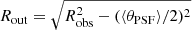 , with ⟨θPSF⟩ being the average PSF FWHM; see Table 2). We thus obtained intrinsic radii of a few kiloparsec for spatially resolved outflows (Rout∼2–4 kpc). For XID614, where the ionised outflow is marginally resolved, we consider the resulting value as an upper limit to Rout (i.e. Rout < 1.9 kpc). All Rout estimates and upper limits are listed in Table 3.
For a measurement of the [O III] flux associated with ionised winds, we followed the prescriptions adopted by Kakkad et al. (2020) for the SUPER type-1 AGN. We hence considered the total [O III] flux contained in the high-velocity line channels (i.e. |v|> 300 km s−1) by summing the flux contributions of all spaxels with S/N > 3 on [O III]. Considering the quality of our data, a non-parametric approach is more suitable than a parametric one based on the results from the multi-Gaussian modelling, where the detection of a broad outflow component depends on the S/N of the data. Because the S/N is low, the [O III] line profile in XID419 is sufficiently well reproduced by a single Gaussian component across the FoV, and no additional component is required. The f300 ratio map shown in Fig. 4 unveils a non-negligible fraction (that varies within 0.3–0.5) of [O III] flux in the |v|> 300 km s−1 line channels, however. This suggests overall that high-velocity gas is outflowing in this galaxy as well (as discussed in Sect. 4.1). However, we point out that by summing the flux of the broad Gaussian components (for the six objects requiring a multi-Gaussian modelling of [O III]) spaxel by spaxel, we obtained [O III] outflow fluxes close to our non-parametric estimates. They differed by a factor of about 2 on average (this was also found in Kakkad et al. 2020 for type-1 AGN).
Finally, we corrected all inferred (non-parametric) [O III] outflow fluxes for dust extinction using the AV values inferred in Sect. 3.2 (see Table 3), and we converted them into intrinsic [O III] outflow luminosities ![Mathematical equation: $ L^{\mathrm{[OIII]}}_{\mathrm{out}} $](/articles/aa/full_html/2024/10/aa50162-24/aa50162-24-eq30.gif) . All resulting dust-corrected
. All resulting dust-corrected ![Mathematical equation: $ L^{\mathrm{[OIII]}}_{\mathrm{out}} $](/articles/aa/full_html/2024/10/aa50162-24/aa50162-24-eq31.gif) values are also reported in Table 3.
values are also reported in Table 3.
4.2.2. Ionised outflow mass rate
The three quantities that were directly measured in the previous subsection (namely, vout, Rout, and ![Mathematical equation: $ L^{\mathrm{[OIII]}}_{\mathrm{out}} $](/articles/aa/full_html/2024/10/aa50162-24/aa50162-24-eq32.gif) ) are fundamental ingredients for computing the mass rate of ionised outflows. Following the prescriptions adopted by Kakkad et al. (2020) for the SUPER type-1 AGN sample, we calculated the ionised outflow masses Mout as follows (for an electron temperature of T ∼ 104 K; e.g. Carniani et al. 2015; Kakkad et al. 2016):
) are fundamental ingredients for computing the mass rate of ionised outflows. Following the prescriptions adopted by Kakkad et al. (2020) for the SUPER type-1 AGN sample, we calculated the ionised outflow masses Mout as follows (for an electron temperature of T ∼ 104 K; e.g. Carniani et al. 2015; Kakkad et al. 2016):
![Mathematical equation: $$ \begin{aligned} M_{\rm out} = 0.8\times 10^8~\bigg ( \frac{L^\mathrm{[O III]}_{\rm out}}{10^{44}~\mathrm{erg\,s}^{-1}} \bigg )~\bigg ( \frac{n_{\rm e}}{500~\mathrm{cm}^{-3}} \bigg )^{-1}~\frac{\mathrm{M}_\odot }{10^\mathrm{[O/H]}}, \end{aligned} $$](/articles/aa/full_html/2024/10/aa50162-24/aa50162-24-eq33.gif) (1)
(1)
where all oxygen was assumed to be ionised to O2+, and ne and [O/H] are the electron density and oxygen abundance in solar units, respectively. For a uniformly filled (i.e. constant ne) outflow with a bi-conical geometry, the mass rate Ṁout at a certain radius Rout can be then calculated as (Fiore et al. 2017)
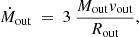 (2)
(2)
which gives the instantaneous mass rate of ionised gas that crosses a spherical sector at a distance Rout from the central AGN.
Equation (1) requires the values of [O/H] and ne, but none of them can be measured from our data. In principle, ne can be inferred from the [S II]λ6716/[S II]λ6731 flux ratio (e.g. Osterbrock & Ferland 2006), but [S II] is undetected in our SINFONI K-band data, except for some faint [S II] emission in XID36 (see Fig. 1). Therefore, we assumed a solar [O/H] abundance and ne = 500 ± 250 cm−3 (i.e. 50% uncertainty), which agrees with previous studies (e.g. Storchi-Bergmann et al. 2010; Carniani et al. 2015; Riffel et al. 2015; Davies et al. 2020; Cresci et al. 2023) and is consistent with the prescriptions adopted in Kakkad et al. (2020) for SUPER type-1 AGN.
In Table 3, we summarise the properties of the ionised outflows in the seven SUPER type-2 AGN with the corresponding uncertainties. We also list the escape velocity vesc from the total galaxy gravitational potential, computed at Rout (see Sect. 5.2) and the AV estimates (or lower limits, derived in Sect. 3.2) we used to obtain the corresponding dust-corrected ![Mathematical equation: $ L^{\mathrm{[OIII]}}_{\mathrm{out}} $](/articles/aa/full_html/2024/10/aa50162-24/aa50162-24-eq35.gif) measurements (or lower limits). The errors vout, w80, and vmax are the uncertainties resulting from the kinematic analysis, while those on AV,
measurements (or lower limits). The errors vout, w80, and vmax are the uncertainties resulting from the kinematic analysis, while those on AV, ![Mathematical equation: $ L^{\mathrm{[OIII]}}_{\mathrm{out}} $](/articles/aa/full_html/2024/10/aa50162-24/aa50162-24-eq36.gif) , and Ṁout were computed via error propagation. Due to the asymmetric uncertainty on AV for cid_1143, the errors on the
, and Ṁout were computed via error propagation. Due to the asymmetric uncertainty on AV for cid_1143, the errors on the ![Mathematical equation: $ L^{\mathrm{[OIII]}}_{\mathrm{out}} $](/articles/aa/full_html/2024/10/aa50162-24/aa50162-24-eq37.gif) and Ṁout for this object correspond to the minimum-maximum range of possible values, which was determined by the minimum/maximum values of the physical quantities on which they depend. Although it is unclear how an uncertainty on Rout is to be estimated, we do not expect errors smaller than the SINFONI spatial pixel (i.e. 0.05″), which corresponds to about 0.4 kpc at z ∼ 2. Nevertheless, the uncertainty on Ṁout is dominated by the large errors on AV (larger than 50%) and ne (assumed equal to 50%). Finally, we note that the inferred upper limit to Rout in XID614 leads to a corresponding lower limit to Ṁout (i.e. Ṁout > 1.7 M⊙ yr−1).
and Ṁout for this object correspond to the minimum-maximum range of possible values, which was determined by the minimum/maximum values of the physical quantities on which they depend. Although it is unclear how an uncertainty on Rout is to be estimated, we do not expect errors smaller than the SINFONI spatial pixel (i.e. 0.05″), which corresponds to about 0.4 kpc at z ∼ 2. Nevertheless, the uncertainty on Ṁout is dominated by the large errors on AV (larger than 50%) and ne (assumed equal to 50%). Finally, we note that the inferred upper limit to Rout in XID614 leads to a corresponding lower limit to Ṁout (i.e. Ṁout > 1.7 M⊙ yr−1).
Before SUPER, the galaxy cid_415 was observed with SINFONI in AO-mode, but with the largest 0.250″ pixel-scale and the lower spectral-resolution HK filter (R ∼ 1500). We note that our inferred values of Rout and vout (Rout ∼ 2.6 kpc and vout ∼ 950 km s−1) are both lower than those reported previously (Rout ∼ 5 kpc and vout ∼ 1600 km s−1; Perna et al. 2015a) based on these first SINFONI datasets. The lower value of Rout is likely a consequence of a surface brightness loss in our SINFONI data as a result of the smaller pixel (0.100″) adopted in SUPER. Instead, the discrepancy in vout is due to a more extreme definition of the outflow velocity adopted in Perna et al. (2015a) (i.e. v05), also combined with slightly different inferred redshifts (z = 2.444 in this work against z = 2.45 in Perna et al. 2015a), which leads to a systematic difference of ∼520 km s−1 in the adopted systemic galaxy velocity (with respect to which all velocities are computed). When we account for these discrepancies, the two vout values are consistent.
5. Comparison with SUPER type-1 active galactic nuclei
In addition to presenting results for the ionised outflows in SUPER type-2 AGN, this paper investigates ionised wind properties as a function of AGN properties (i.e. the AGN bolometric luminosity Lbol and the hydrogen column density NH) and host galaxy parameters (i.e. the stellar mass M*, the star formation rate, and the escape velocity vesc) for the full SUPER sample with the aim to unveil any difference between type-1 and type-2 systems. The difference might shed light on the intrinsic nature of these two AGN classes. Except for vesc (see Sect. 5.2) and NH (measured from archival X-ray spectra, Circosta et al. 2018), all other AGN or host galaxy properties were derived by Circosta et al. (2018) using the SED fitting code called Code Investigating GALaxy Emission (CIGALE; Noll et al. 2009), and are overall confirmed by the latest updates presented in Bertola et al. (2024). The values of M*, of the star formation rate (SFR), of Lbol and of NH for the SUPER type-2 AGN are listed in Table 1 (see Kakkad et al. 2020 for the type-1 AGN).
5.1. Faster outflows in type-2 active galactic nuclei at the low-luminosity end
The key result of this work is shown by the three panels of Fig. 8, which overall display the outflow velocity as a function of AGN bolometric luminosity Lbol for the full SUPER sample, divided into type-2 (coloured thick crosses) and type-1 (grey squares) AGN. In particular, in the left and middle panels, vout = max[|v10|,|v90|] and vmax = vbro + 2σbro are displayed along the y-axis. The type-1 AGN measurements were taken consistently from Kakkad et al. (2020). In addition to showing the well-known trend of a higher outflow velocity at increasing AGN luminosity (e.g. Bae & Woo 2014; Woo et al. 2016; Perna et al. 2017; Rakshit & Woo 2018; discussed in Sect. 6), both panels consistently show the same following result in the lower Lbol regime (i.e. Lbol ∼ 1044.8 − 46.5 erg s−1; orange shading), where all SUPER type-2 AGN are found. Interestingly, the SUPER type-2 AGN host overall faster ionised outflows than their type-1 counterparts within the same Lbol range, and they appear to depart from the global vout, max − Lbol increasing trend followed by the SUPER type-1 AGN. As expected, the vmax value of XID419 is the lowest of the type-2 sample because vmax for this target is computed as 2σ (see Sect. 4.2.1), where σ refers to the single-Gaussian component we employed.
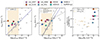 |
Fig. 8. Outflow velocities vout and vmax (left and middle panels) as a function of Lbol, and vout/Lbol ratios vs. X-ray NH measurements (right panel). The coloured crosses and grey squares represent SUPER type-2 and type-1 AGN, and the triangles in the right panel indicate upper and lower limits to NH. The dash-dotted blue lines represent our best-fit linear relation to the type-1 measurements, from which the type-2 points depart increasingly at decreasing Lbol (the mean deviation is 0.4dex). In the middle panel, we draw the empirical relation by Fiore et al. (2017) for comparison (dotted line), along with a more recent version from Musiimenta et al. (2023) (dashed). The orange shading in the left and middle panels marks the low-Lbol range (i.e. Lbol = 1044.8 − 46.5 erg s−1), where we compare the type-1 and type-2 AGN measurements. In the right panel, we consistently use light orange markers to identify type-1 AGN in the low-Lbol regime. |
To better appreciate the deviation in the type-2 velocity measurements from the type-1 ones, we fitted a linear relation to the type-1 distribution in the vout − Lbol and vmax − Lbol planes (dash-dotted blue line), from which type-2 velocities deviate increasingly at lower luminosities by up to about 0.8 dex in both panels, and with a mean deviation of 0.4 dex. In the middle panel, we also draw the empirical vmax − Lbol relation inferred in Fiore et al. (2017) for comparison (dotted black line) and an updated version by Musiimenta et al. (2023) (dashed black line) that includes recent results and only considers z > 0.5 AGN. The type-1 population appears to overall follow the empirical relation by Musiimenta et al. (2023), as opposed to the type-2 measurements. We point out that the small number (i.e. seven) of type-2 measurements prevents us from an accurate linear fit to the type-2 distribution of measurements.
In Appendix A we show additional plots in which we compare other outflow properties and AGN and host galaxy parameters, none of which indicate either a clear trend or an interesting discrepancy between the type-1 and type-2 populations in SUPER. In particular, the left and right panels of Fig. A.1 display vout plotted against M* and SFR, whereas in Fig. A.2 we searched for trends in the outflow mass rate with Lbol. Although the vout − Lbol plane reveals a clear dichotomy of type-1 and type-2, it is hard to establish whether the two AGN populations are also separated in terms of the outflows mass rate because the uncertainty on this quantity is large. The mass rate estimates strongly depend on the accuracy of other measured parameters (e.g. AV and Rout), and they also require several quantities to be assumed (e.g. ne, [O/H], and ionisation). All these uncertainties inevitably increase the scatter in the resulting mass-rate values, and thus possibly hide the type-1 to type-2 dichotomy that is instead visible in terms of the more directly inferred outflow velocities.
We investigate the potential effect of different nuclear obscuring conditions on driving the outflows in the right panel of Fig. 8 with the aim to shed light on the nature of the dichotomy of type-1 and type-2 that we discovered. To remove any dependence of vout on the AGN luminosity (discussed in Sect. 6), we normalised vout to Lbol (in units of 1045 erg s−1), and we plot the resulting vout/Lbol ratios against the hydrogen column density NH, measured from X-ray data in Circosta et al. 2018 for the full SUPER sample. Light orange markers identify type-1 AGN lying in the low-Lbol regime (i.e. Lbol ∼ 1044.8 − 46.5 erg s−1, orange shading in the left and middle panels), and high-Lbol type-1 objects are plotted as grey markers. The upper and lower limits to NH are finally shown as triangles. The right panel clearly shows that SUPER type-1 and type-2 AGN occupy two distinct regions of the (vout/Lbol)−NH plane. The distribution of SUPER measurements along the x-axis shows their X-ray obscured and unobscured classification (see Circosta et al. 2018). All SUPER type-2 AGN lie in the highly obscured X-ray regime (NH ≳ 1023 cm−2), whereas most of the type-1 population exhibits unobscured conditions (NH ≲ 1022 cm−2), with some systems lying in the intermediate-obscuration region (NH ∼ 1022 − 1023 cm−2). The combined resulting separation along the y-axis is more interesting and unexpected: the SUPER type-2 sample indeed features vout/Lbol values that vary within ∼30–1500 (and only cid_451 is lower than 80), with a mean value of ∼400, while almost all type-1 AGN have ratios lower than 50, with an overall mean value of ∼40. This shows a picture in which AGN-driven outflows are accelerated more efficiently in more obscured environments (this is further discussion in Sect. 6).
To further verify and quantify the observed discrepancy in the outflow velocity between SUPER type-1 and type-2 AGN, we directly compared the mean [O III] line profiles of SUPER type-1 and type-2 AGN by separately stacking [O III] integrated spectra of the type-1 and type-2 objects with Lbol ∼ 1044.8 − 46.5 erg s−1 (Fig. 9): these are all 7 type-2 AGN and 11 type-1 systems (i.e. those lying within the orange shading of Fig. 8). The selection of objects over this broad (about two orders of magnitude) luminosity range ensured that we accounted for possible over- or underestimates of Lbol from the SED fitting in type-2 AGN (Circosta et al. 2018) because fainter AGN emission is hard to constrain. However, we confirmed the reliability of the SED-based measurements for the type-2 AGN by also estimating Lbol from the dust-corrected [O III] luminosity (Lamastra et al. 2009) and from the X-ray 2–10 keV luminosity (Duras et al. 2020). We thus find that the Lbol values derived from the SED fitting agree with the [O III]-based estimates within a factor of 2 on average (computed for the four objects with AV estimates; see Table 3) and from the X-ray-based values by a mean factor of 4, without obvious biases towards higher or lower Lbol with respect to the SED fitting derivation.
For each selected AGN, we extracted an integrated [O III]λ5007 spectrum using an aperture with a radius of 0.25″ after removing continuum emission in SUPER type-2 datacubes (see Sect. 3.1) and continuum+BLR emission in type-1 datacubes (Kakkad et al. 2020). We excluded spectra with an S/N < 5 on [O III] from the stack to allow for a more accurate comparison of line profiles. We thus finally had six S/N > 5 type-2 spectra (all but XID419) and six S/N > 5 type-1 spectra (X_N_66_23, X_N_115_23, cid_467, S82X1905, S82X1940, and S82X2058). Each type-1 and type-2 spectrum was weighted by the inverse of its squared noise before it was added to the stack, and then the final stacked type-2 and type-1 spectra (red and blue spectra in Fig. 9, respectively) were normalised to the resulting respective [O III] peak. We point out that results similar to those described below are obtained even by stacking unweighted spectra. In Fig. 9, we show the resulting stacked [O III] line profiles of the selected type-2 (red) and type-1 (blue) SUPER AGN using a binning that is twice larger than SINFONI spectral channel to remove noisier channels. The type-2 [O III] line profile exhibits more prominent blue and red wings than the type-1 spectrum. Via multiple stacks of type-2 integrated spectra, each time excluding one object, we verified that all type-2 objects contribute to the [O III] blue wing, whereas the red wing is dominated by XID36. Because of the brighter and more prominent blue wing, the type-2 [O III] line profile also appears to be more asymmetric than that of type-1.
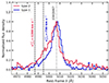 |
Fig. 9. Stacked [O III]λ5007 spectra of type-2 (red) and type-1 (blue) AGN from SUPER with Lbol ∼ 1044.8 − 46.5 (orange shading in Fig. 8), resulting from integrated (aperture with a radius of 0.25″), subtracted [O III] spectra with S/N > 5. The integrated spectra were averaged by the inverse of the squared noise, and then the resulting stacked spectrum was normalised to the final [O III] peak. Comparing the two stacked spectra, we find a statistically significant (2.7σ) difference in the [O III] blue wing, which is more prominent in the type-2 spectrum of about 500 km s−1 compared to the type-1 stack. |
We measured the v10 velocity of each resulting stacked type-1 and type-2 spectrum (vertical dashed lines in Fig. 9) and quantified the corresponding uncertainty as the standard deviation of the v10 distribution resulting from a bootstrap of 400 stacks of six type-1 and type-2 spectra, randomly selected with an equal probability and allowing for repetitions. We thus obtained 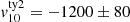 km s−1 for the type-2 line profile and
  km s−1 for the type-1 spectrum (see Fig. 9), corresponding to a 2.7σ difference in the [O III] blue wing of the AGN samples. We note that the identification of extended [O III] wings at high velocity is generally more challenging in type-1 AGN than in type-2 systems because of the bright BLR emission (i.e. Hβ and Fe II) in the [O III] wavelength range. Therefore, to verify the goodness of the BLR and continuum modelling of the SUPER type-1 AGN, we also stacked type-1 spectra without removing BLR emission (i.e. only continuum emission was removed), employing the best-fit results from Kakkad et al. (2020). We find that no evident Fe II emission bumps are present in correspondence of the [O III] line wings, and that the bulk of BLR emission in this spectral region is due to extremely large red wings of the Hβ BLR line component (see Figs. A.1–A.4 in Kakkad et al. 2020). This supports the reliability of our comparison between type-1 and type-2 stacked spectra (see Fig. 9) and furthermore strengthens our result of a type-1 and type-2 dichotomy in ionised outflow velocity, as firstly pointed out by our spatially resolved measurements (shown in Fig. 8). The origin of this observed difference, revealing faster ionised outflows in type-2 AGN, is discussed in Sect. 6.
5.2. Can ionised outflows escape the galaxy gravitational potential?
One of the main channels via which outflows can quench (or at least reduce) galactic SF is through the ejection of a substantial amount of gas from the host galaxy that would otherwise be available to form new stars. This requires outflows that are energetic enough to efficiently sweep away the gas on large scales, eventually escaping the gravitational potential of their galaxy. Kakkad et al. (2020) presented a first investigation of the ejective ability of the ionised outflows detected in the SUPER type-1 sample and found that for most galaxies, only a modest fraction (< 10%) of the outflowing gas can effectively escape the gravitational potential well of the host. In this section, we compare the outflow velocities with the escape velocity of each galaxy for the full SUPER sample for all objects with a more accurate mass modelling.
Following prescriptions from the literature (Marasco et al. 2023), we used the python package galpy (Bovy 2015) to build a dynamical mass model consisting of a dark matter (DM) halo, a stellar disk, and a gaseous disk, to derive the total escape velocity profile for SUPER targets with a known M*, derived from SED fitting (Circosta et al. 2018). All examined type-2 AGN galaxies have M* estimates ranging within M* ∼ 1010.7 − 11.2 M⊙ (see Table 1), while for only a few type-1 systems, M* estimates are available (M* ∼ 1010.1 − 11.2 M⊙). The stellar emission is typically buried in the bright AGN component of type-1 systems and thus prevents us from constraining M* in most cases (only six SUPER type-1; see Table A.2 in Circosta et al. 2018).
For the DM halo, we assumed a Navarro-Frenk-White (NFW, Navarro et al. 1997) profile, with a virial mass M200 derived from M* via the stellar-to-halo mass relation of Girelli et al. (2020), and a concentration c determined from the M200 − c relation of Dutton & Macciò (2014); both relations were computed at the redshift of each target. We modelled the stellar disk with a double-exponential profile with scale-length Rd and scale height Rd/5, assuming Rd equal to the half-light radius R50 divided by 1.68 (correct for a purely exponential disk, Sérsic index n = 1). We determined R50 from the size-M* relation for a disk galaxy (n = 1) at z ∼ 2.2 (Mowla et al. 2019). Since we have CO-based measurements of molecular gas mass Mgas for a few SUPER AGN (Circosta et al. 2021), we modelled a gaseous disk of Mgas equal to the mean value measured for SUPER targets (i.e. Mgas ∼ 6 × 10⁹ M⊙) and the same size as the stellar disk, since we expect the molecular gas to extend on scales comparable to those of stars. In this way, we derived the escape velocity profile of the total modelled mass distribution (i.e. DM halo + stellar disk + gas disk).
Figure 10 displays vout as a function of the escape velocity at the maximum inferred outflow radius Rout for SUPER type-2 (coloured symbols) and all those type-1 (grey) AGN with known M* (Circosta et al. 2018), hence not Lbol-matched to the type-2 AGN sample. The two panels display data points corresponding to two distinct definitions of escape speed: one speed derived according to the classical definition6 (vesc in the left panel; also listed in Table 3), which translates in more practical terms into the velocity needed to reach the virial radius Rvir of the DM halo, as derived from our mass modelling (Rvir ∼ 80 − 160 kpc); and the other speed corresponding to a less rigid definition of the escape speed ( in the right panel), namely the velocity required to reach 10 Re (i.e. ∼30–50 kpc, depending on the galaxy). This second set of values shows whether the outflows can travel up to distances of tens of kiloparsec from the centre of the galaxy, and escape (at least) the gravitational potential of the galaxy baryonic component (i.e. stellar disk + gas disk). The triangles indicate lower limits to the escape speed, corresponding to upper limits to Rout, since the escape speed curves increase at decreasing Rout. A dashed line indicates the locus of points where vout are equal to the escape speed values. Under the simplifying assumption that our dynamical modelling introduces no further uncertainty, we consider the error on our escape speed values to be due to the total uncertainty on M*, including both statistical (from SED fitting Circosta et al. 2018) and systematic (∼0.1 dex; Pacifici et al. 2023) uncertainties.
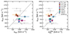 |
Fig. 10. Outflow velocity vout as a function of escape velocity computed at Rout, as inferred from our mass modelling of SUPER type-2 (coloured symbols) and all those type-1 (grey) AGN galaxies with a known M*, hence not Lbol-matched to the type-2 AGN sample. We display two sets of escape speed values: One value was inferred according to the classical definition of the escape velocity to infinity (vout, left panel), hence, this needed to escape the DM halo (Rvir ∼ 80 − 160 kpc); the other value corresponded to the escape velocity required to reach 10 Re ( |


In the left panel of Fig. 10, the overall majority of galaxies has vout values consistent or nearly consistent with vesc to infinity. Unfortunately, the uncertainties and simplified assumptions of our dynamical modelling prevent us from firmly testing whether these outflows can effectively sweep up a significant amount of gas out of the DM halo, as predicted by the ejective feedback scenario. We derived the outflow velocity (assumed to be constant in our model) from our observed velocity measurements, which are subject to inclination effects and limited to a few kiloparsec from the centre of each galaxy, beyond which the line emission becomes fainter and the S/N drops. Moreover, our dynamical model only includes gravity and no hydrodynamic effects, which may instead play a major role. Outflows could hence become trapped in gaseous haloes, eventually cool, and be re-accreted, even if they have high initial velocities. This would contribute to hampering the wind ejective ability to expel the gas reservoir of their host, unlike model predictions (e.g. King & Pounds 2015; Zinger et al. 2020). The distribution of measurements in the right panel of Fig. 10 strongly suggests, however, that even if these outflows do not successfully escape the total gravitational potential well (i.e. the DM halo), they are likely to impact the host gas reservoir up to galaxy scales (i.e. 30–50 kpc). They can hence sweep gas out of the galaxy disk and/or provide feedback through a preventive mode (e.g. van de Voort et al. 2011) by injecting energy and driving turbulence in the surrounding medium. All this will eventually prevent gas from cooling and collapsing to form new stars. Even when we infer escape speeds at a fixed radius of 50 kpc for all galaxies, we obtain escape speeds similar to  . Finally, as opposed to Fig. 8, we note that Fig. 10 shows no clear separation between type-1 and type-2 AGN measurements.
6. Discussion
Our analysis has unveiled that SUPER type-2 AGN host faster ionised outflows than their type-1 counterparts in the lower Lbol regime (Lbol ∼ 1044.8 − 46.5), as traced by higher [O III] velocities. At low redshift (z < 0.8), several studies have searched for differences in the ionised outflow properties between type-2 and type-1 systems in large AGN samples (e.g. Mullaney et al. 2013; Bae & Woo 2014; Rakshit & Woo 2018; Wang et al. 2018; Rojas et al. 2020). In general, they found narrower and more symmetric [O III] line profiles in type-2 AGN, indicating the detection of both blueshifted and redshifted outflow components, and almost exclusively blueshifted outflows in type-1 AGN, with typically larger line widths and more negative velocities. This can be explained in terms of biconical outflow geometry in the context of standard unification models (e.g. Antonucci 1993; Urry & Padovani 1995) as a consequence of orientation effects along the line of sight, combined with dust obscuration. When we assume a nearly face-on orientation of type-1 AGN, with clearly visible BLR emission along the line of sight, the receding cone of the outflow remains hidden on the opposite side of the galaxy disk plane.
However, most of these low-redshift studies did not consider the well-known dependence of the outflow kinematics on the AGN luminosity and accretion rate (e.g. Bae & Woo 2014; Woo et al. 2016; Rakshit & Woo 2018), and they overall compared more luminous type-1 AGN with fainter type-2 samples, which might have led to an only apparent discrepancy. Moreover, current observational evidence increasingly challenges the standard unified picture of AGN, such as the discovery of changing-look AGN (see Ricci & Trakhtenbrot 2023 for a recent review), which favours the interpretation of the dichotomy between type-1 and type-2 AGN in terms of distinct phases within a common evolutionary sequence.
At high redshift (z > 1), where more complex processes are expected to take place, especially at crucial cosmic epochs of galaxy evolution such as z ∼ 2, orientation effects might play a minor role compared to low redshift. Previous works have indeed provided evidence that the bulk of the dust obscuration at high redshift comes from the host galaxy and is not caused by the classical dusty torus (e.g. Gilli et al. 2014, 2022; Perna et al. 2018; Circosta et al. 2019). This is consistent with results from numerical simulations, according to which different AGN classes correspond to distinct evolutionary phases of in the life cycle of galaxies (Hopkins et al. 2006; Menci et al. 2008). In particular, X-ray bright but obscured (L2 − 10 keV > 1044 erg s−1, NH ≳ 1022 cm−2) AGN at z ∼ 2 have been proposed to be in the active blow-out phase in the evolution of AGN galaxies (e.g. Brusa et al. 2010; Urrutia et al. 2012), and powerful outflows have been detected in these systems (e.g. Brusa et al. 2015, 2016; Zakamska et al. 2016; Perna et al. 2015a,b; Vayner et al. 2023; Glikman et al. 2024). In these obscured sources, dusty material favours the acceleration of outflows (e.g. Ishibashi & Fabian 2015; Costa et al. 2018), which efficiently clear out obscuring dust and finally unveil the AGN. Radiation pressure on dust has been indeed identified as the main mechanism that causes the higher [O III] velocities and line widths that are observed in extremely red and luminous quasars (ERQs; Lbol > 1047 erg s−1) compared to blue quasars at z = 2 − 3 (Perrotta et al. 2019).
However, Villar Martín et al. (2020) provided a revised comparison of the [O III] kinematics in 20 ERQs from Perrotta et al. (2019) with other AGN samples that matched in luminosity, and found the [O III] velocities of ERQs to be overall consistent with those of luminous blue quasars. A similar result was also found by Temple et al. (2019), who compared the [O III] kinematics in a sample of luminous (Lbol ≈ 1047 erg s−1) highly reddened quasars at z > 2 to unobscured quasars in the same luminosity and redshft range. In contrast, higher [O III] velocities have been observed by DiPompeo et al. (2018) in obscured AGN at z < 0.4, resembling the obscured high-redshift population based on their optical/IR colours, and matched in luminosity with unobscured objects. All these controversial results show how complex it is to carry out such a comparison, and it leaves the debate open.
Figure 11 displays the same panels as Fig. 8 and compares the results obtained for SUPER targets with measurements from the literature. In particular, we collected from the literature only results based on IFS observations and with outflow velocities that were defined consistently with ours in SUPER to allow for a proper comparison that was as homogeneous as possible. In all three panels of Fig. 11, SUPER results of type-2 and type-1 AGN are shown as filled red and blue markers, respectively, along with other IFS-based measurements of type-2 (empty red star; XID5395, Brusa et al. 2016) and type-1 (empty blue symbols; Cano-Díaz et al. 2012; Carniani et al. 2015; Vayner et al. 2021a) AGN at z = 1 − 3 from the literature. In orange, we highlight the measurements relative to red obscured AGN showing BLR emission (hence, optical type-1 systems), which should be considered as an intermediate class of objects between standard (blue) type-1 and (red) type-2 AGN. These are the obscured quasar XID2028 at z ∼ 1.6 (empty orange pentagon; Cresci et al. 2023; Veilleux et al. 2023), the powerful obscured ERQs from Perrotta et al. (2019) (empty orange circles); and the sample of obscured quasars from Vayner et al. (2021b) (orange diamonds), among which all but one (the lowest-velocity point) are selected as ERQs.
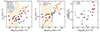 |
Fig. 11. Same panels as in Fig. 8, showing SUPER type-2 (filled red circles) and type-1 (filled blue circles) measurements along with IFS-based results from the literature of other type-2 (empty red star; XID5395, Brusa et al. 2016) and type-1 AGN (empty blue symbols; Cano-Díaz et al. 2012; Carniani et al. 2015; Vayner et al. 2021a) at z ∼ 1 − 3. The orange symbols represent red obscured systems that were nevertheless optically classified as type-1 AGN (Perrotta et al. 2019; Vayner et al. 2021b; Cresci et al. 2023; Veilleux et al. 2023). Outflow velocities from Brusa et al. (2016) and Perrotta et al. (2019) have been corrected to account for discrepancies with the vout and vmax definitions we adopted (see Sect. 6). While the ‘standard’ blue type-1 and red type-2 from the literature agree with values found in SUPER, the orange points, almost all at Lbol ≳ 1047 erg s−1, clearly show that higher outflow velocities are recovered when we select optical type-1 but dusty obscured objects. |
The first panel compares vout measurements from SUPER and the literature based on v10/v90, as obtained by Vayner et al. (2021a,b) (blue/orange diamonds) and by Cresci et al. (2023) and Veilleux et al. (2023) consistently for XID2028, and higher percentile outflow velocities were used in Brusa et al. (2016) and Perrotta et al. (2019) (i.e. v05 and v02, respectively). Therefore, we corrected the outflow velocities inferred in Brusa et al. (2016) and Perrotta et al. (2019) by a factor of 0.86 and 0.77, respectively, corresponding to the mean ratio of v10, 90 to v05, 95 and v10, 90 to v02, 98 measured for SUPER type-2 AGN. We also added measurements from Cano-Díaz et al. (2012) and Carniani et al. (2015). Similarly, we re-scaled the v02 outflow velocities from Perrotta et al. (2019) by a factor of 1.2, as obtained from the mean vmax-to-v02, 98 ratio for SUPER type-2 AGN, and plot them in the vmax − Lbol plane (middle panel), along with vmax measurements for SUPER type-2 (derived in Sect. 4.2.1) and type-1 AGN (Kakkad et al. 2020).
As shown in Fig. 11, standard blue (unobscured) type-1 and red (obscured) type-2 AGN from the literature lie close to SUPER type-1 and type-2 points, respectively. For instance, the obscured type-2 AGN XID5395 (empty red star; Brusa et al. 2016) exhibits an outflow velocity and vout/Lbol ratio (i.e. ∼130) that is comparable with those of SUPER type-2 systems, and a column density (NH ∼ 1023 cm−2) that places this source in the nuclear highly obscured regime. Within the optical type-1 AGN population, we instead note that hybrid sources (i.e optical type-1 but X-ray obscured AGN; orange markers) show higher outflow velocities, consistently with the picture proposed in this work. The hybrid type-1 AGN XID2028 (empty pentagon; Perna et al. 2015b; Cresci et al. 2023; Veilleux et al. 2023) behaves like the SUPER type-2 objects in terms of vout − Lbol, but it is more similar to SUPER type-1 counterparts in the vout/Lbol − NH parameter space, falling at the boundary of the obscured versus unobscured regimes (NH ∼ 1022 cm−2).
Therefore, radiation pressure of dust might be the dominant mechanism to explain the presence of faster-ionised outflows in type-2 AGN, also at a lower bolometric luminosity than is typical of ERQs (Lbol > 1047 erg s−1) from Perrotta et al. (2019). Our analysis has furthermore revealed a clear dichotomy between type-1 and type-2 AGN that fully reflects the classification into X-ray unobscured and obscured sources based on obscuring material on nuclear scales. Interestingly, the SUPER type-2 AGN are all highly X-ray obscured, with NH ≳ 1023 cm−2, which may explain that the observed velocities of their ionised outflows are higher than those observed in SUPER type-1 AGN within the same luminosity range. Rather than being a consequence of projection effects, this result supports the scenario in which obscured optical type-2 AGN at z ∼ 2 might indeed evolve towards the unobscured type-1 phase, as radiation-pressure driven outflows blow out obscuring material and unveil the central AGN and its BLR emission.
Even though previous studies have pointed to individual sources as likely blow-out candidates (e.g. Brusa et al. 2016), SUPER has provided observational evidence of this evolutionary scenario in a larger AGN sample, and also showed for the first time an optical dichotomy of type-1 and type-2 AGN in outflow velocity in a sample of moderately luminous AGN at z ∼ 2 (i.e. Lbol ∼ 1044.8 − 46.5 erg s−1). As a comparison, the ERQ sample at z = 2 − 3 studied by Perrotta et al. (2019) consists of highly luminous AGN (Lbol > 1047 erg s−1), all with BLR emission (hence, optical type-1 systems). On the other hand, the published results from the KASHz survey (Harrison et al. 2016) relative to X-ray-selected AGN (L2 − 10 keV > 1042 erg s−1) at z = 0.6 − 1.7 shows no evidence for more extreme gas kinematics in obscured (type-2) objects than in their unobscured (type-1) counterparts (see the left panel of Fig. 8). We point out that this is likely a consequence of the lower S/N of the KASHz data compared to SUPER, which hampers the detection of any extended [O III] line wing. This is indeed the case for cid_1143 and cid_451, which are targets in common to both surveys (Scholtz et al., in prep.), where the shallower KMOS data completely miss the broad [O III] wing due to the outflow, thus underestimating its velocity.
7. Conclusions
We presented SINFONI H- and K-band observations of the SUPER type-2 AGN sample, thus complementing the previously reported results on the type-1 systems (Kakkad et al. 2020, 2023). The spectral analysis of SINFONI datacubes (Sect. 3.1) allowed us to study the spatial distribution and kinematics of ionised gas via [O III] line emission (Sect. 4.1), and we found evidence for ionised outflows in all seven examined type-2 AGN that move at vout > 600 km s−1. The detected outflows are spatially resolved in six objects and extend up to 2–4 kpc from the centre, and they are marginally resolved in the remaining source (XID614, Rout < 1.9 kpc). We also computed outflow mass rates from the dust-corrected [O III] outflow luminosity (Sect. 4.2.2).
In Sect. 5, we investigated the outflow velocity as a function of AGN bolometric luminosity with the aim to unveil any difference between the type-1 and type-2 AGN populations in SUPER. The key result of this paper is presented in Sect. 5.1 and is clearly shown in Fig. 8, where the outflow velocity is plotted against Lbol: SUPER type-2 AGN host faster winds than the type-1 systems within the same luminosity range (i.e. Lbol = 1044.8 − 46.5 erg s−1). Interestingly, these type-2 AGN (namely, all type-2 systems with a high-S/N [O III] detection in our SINFONI observations) are all highly obscured systems (NH ≳ 1023 cm−2). By separately stacking integrated type-1 and type-2 spectra, we found a 2.7σ difference in the blue wing of the [O III] line profile, which appears to be more prominent in type-2 AGN than in their type-1 counterparts (Fig. 9). We interpret this as a consequence of the larger amount of obscuring material (NH ≳ 1024 cm−2 in all examined type-2 AGN), which favours the acceleration of winds via radiation pressure on dust (e.g. Ishibashi & Fabian 2015; Costa et al. 2018).
The SUPER survey has hence provided observational evidence of an evolutionary origin of the dichotomoy of type-1 and type-2 AGN at z ∼ 2, which is consistent with theoretical predictions and with previous observational evidence, whereas orientation effects might play a minor role. Within this picture, type-2 AGN represent (even at lower luminosity) the blow-out phase (e.g. Hopkins et al. 2008), whose obscured environment favours the acceleration of fast winds via radiation pressure on dust. This interpretation was proposed before for obscured AGN at z ∼ 2 (e.g. Brusa et al. 2015, 2016; Perna et al. 2015a; Zakamska et al. 2016), but was not clearly associated with the type-2 optical class, with some of these examined X-ray obscured AGN being optical type-1 systems (e.g. Perna et al. 2015b; Perrotta et al. 2019). Moreover, the velocities of the ionised outflows that are overall detected in SUPER AGN galaxies are compatible with the escape speed of their DM halo (Fig. 10, left panel), which does not indicate a dichotomy of type-1 and type-2 AGN, however. Unfortunately, the uncertainties and the simplified assumptions of our dynamical model prevented us from testing the ejective feedback scenario in a concluding way. However, we found that although they might be unable to successfully escape the DM halo of their galaxy, these ionised outflows are likely to reach 30–50 kpc scales (Fig. 10, right panel), where they can still provide effective feedback by sweeping away gas and/or injecting energy in the galaxy medium (preventive mode), thus halting the formation of new stars.
To confirm this novel result found in SUPER, in future we will need larger samples of high-redshift type-1 and type-2 AGN. The new generation of IFS facilities, both from space (e.g NIRSpec on JWST) and on the ground with AO (e.g. ERIS at VLT), will allow us to exploit the power of spatially resolved observations as much as possible to finally take the next step to fully understand feedback mechanisms and AGN evolution at cosmic noon.
K-band Multi Object Spectrograph (Sharples et al. 2013).
Link to the SUPER webpage http://www.super-survey.org/
Compared to the original 39-AGN SUPER sample, six objects were eventually not observed. This was a consequence of time lost because of bad weather conditions because part of the survey was executed in visitor mode rather than in service mode.
The percentile velocities vxx used in the following are defined as the velocity containing xx% of the total [O III] line flux.
The [O III] line emission requires more assumptions than Hα or Hβ, but the latter are overall detected at a lower S/N than [O III], which was the motivation for our choice.
The minimum velocity required by an object to reach to infinity, with a final null velocity.
Acknowledgments
We thank Giacomo Venturi for the insightful discussion and his advise on dynamical mass modelling. We acknowledge financial support from INAF under the Large Grant 2022 “The metal circle: a new sharp view of the baryon cycle up to Cosmic Dawn with the latest generation IFU facilities”. We also acknowledge support from the Italian Ministry for University and Research (MIUR) for the BLACKOUT project funded through grant PRIN 2017PH3WAT.003, and for the project “Black Hole winds and the Baryon Life Cycle of Galaxies: the stone-guest at the galaxy evolution supper”, funded through grant PRIN #2017PH3WAT. MP acknowledges support from Grant PID2021-127718NB-I00 funded by the Spanish Ministry of Science and Innovation/State Agency of Research (MICIN/AEI/ 10.13039/501100011033). CMH acknowledges funding from a United Kingdom Research and Innovation grant (code: MR/V022830/1). IL acknowledges support from PID2022-140483NB-C22 funded by AEI 10.13039/501100011033 and BDC 20221289 funded by MCIU by the Recovery, Transformation and Resilience Plan from the Spanish State, and by NextGenerationEU from the European Union through the Recovery and Resilience Facility. AP acknowledges support by an Anniversary Fellowship at the University of Southampton.
References
- Antonucci, R. 1993, ARA&A, 31, 473 [Google Scholar]
- Arribas, S., Colina, L., Bellocchi, E., Maiolino, R., & Villar-Martín, M. 2014, A&A, 568, A14 [NASA ADS] [CrossRef] [EDP Sciences] [Google Scholar]
- Bae, H.-J., & Woo, J.-H. 2014, ApJ, 795, 30 [NASA ADS] [CrossRef] [Google Scholar]
- Bertola, E., Circosta, C., Ginolfi, M., et al. 2024, A&A, in press https://doi.org/10.1051/0004-6361/202450420 [Google Scholar]
- Bischetti, M., Piconcelli, E., Vietri, G., et al. 2017, A&A, 598, A122 [NASA ADS] [CrossRef] [EDP Sciences] [Google Scholar]
- Bouché, N., Murphy, M. T., Kacprzak, G. G., et al. 2013, Science, 341, 50 [Google Scholar]
- Bovy, J. 2015, ApJS, 216, 29 [NASA ADS] [CrossRef] [Google Scholar]
- Brusa, M., Civano, F., Comastri, A., et al. 2010, ApJ, 716, 348 [NASA ADS] [CrossRef] [Google Scholar]
- Brusa, M., Bongiorno, A., Cresci, G., et al. 2015, MNRAS, 446, 2394 [NASA ADS] [CrossRef] [Google Scholar]
- Brusa, M., Perna, M., Cresci, G., et al. 2016, A&A, 588, A58 [NASA ADS] [CrossRef] [EDP Sciences] [Google Scholar]
- Calzetti, D., Armus, L., Bohlin, R. C., et al. 2000, ApJ, 533, 682 [NASA ADS] [CrossRef] [Google Scholar]
- Cano-Díaz, M., Maiolino, R., Marconi, A., et al. 2012, A&A, 537, L8 [NASA ADS] [CrossRef] [EDP Sciences] [Google Scholar]
- Carniani, S., Marconi, A., Maiolino, R., et al. 2015, A&A, 580, A102 [NASA ADS] [CrossRef] [EDP Sciences] [Google Scholar]
- Carniani, S., Venturi, G., Parlanti, E., et al. 2024, A&A, 685, A99 [NASA ADS] [CrossRef] [EDP Sciences] [Google Scholar]
- Chartas, G., Davidson, E., Brusa, M., et al. 2020, MNRAS, 496, 598 [Google Scholar]
- Cicone, C., Maiolino, R., Sturm, E., et al. 2014, A&A, 562, A21 [NASA ADS] [CrossRef] [EDP Sciences] [Google Scholar]
- Cicone, C., Brusa, M., Ramos Almeida, C., et al. 2018, Nat. Astron., 2, 176 [Google Scholar]
- Circosta, C., Mainieri, V., Padovani, P., et al. 2018, A&A, 620, A82 [EDP Sciences] [Google Scholar]
- Circosta, C., Vignali, C., Gilli, R., et al. 2019, A&A, 623, A172 [NASA ADS] [CrossRef] [EDP Sciences] [Google Scholar]
- Circosta, C., Mainieri, V., Lamperti, I., et al. 2021, A&A, 646, A96 [EDP Sciences] [Google Scholar]
- Civano, F., Marchesi, S., Comastri, A., et al. 2016, ApJ, 819, 62 [Google Scholar]
- Costa, T., Sijacki, D., & Haehnelt, M. G. 2014, MNRAS, 444, 2355 [Google Scholar]
- Costa, T., Rosdahl, J., Sijacki, D., & Haehnelt, M. G. 2018, MNRAS, 479, 2079 [Google Scholar]
- Cresci, G., Mainieri, V., Brusa, M., et al. 2015, ApJ, 799, 82 [Google Scholar]
- Cresci, G., Tozzi, G., Perna, M., et al. 2023, A&A, 672, A128 [NASA ADS] [CrossRef] [EDP Sciences] [Google Scholar]
- Davies, R. I. 2007, MNRAS, 375, 1099 [Google Scholar]
- Davies, R., Rabien, S., Lidman, C., et al. 2008, Messenger, 131, 7 [NASA ADS] [Google Scholar]
- Davies, R., Baron, D., Shimizu, T., et al. 2020, MNRAS, 498, 4150 [Google Scholar]
- DiPompeo, M. A., Hickox, R. C., Carroll, C. M., et al. 2018, ApJ, 856, 76 [Google Scholar]
- Duras, F., Bongiorno, A., Ricci, F., et al. 2020, A&A, 636, A73 [NASA ADS] [CrossRef] [EDP Sciences] [Google Scholar]
- Dutton, A. A., & Macciò, A. V. 2014, MNRAS, 441, 3359 [Google Scholar]
- Eisenhauer, F., Abuter, R., Bickert, K., et al. 2003, SPIE Conf. Ser., 4841, 1548 [Google Scholar]
- Fabian, A. C. 2012, ARA&A, 50, 455 [Google Scholar]
- Fawcett, V. A., Alexander, D. M., Brodzeller, A., et al. 2023, MNRAS, 525, 5575 [CrossRef] [Google Scholar]
- Ferrarese, L., & Merritt, D. 2000, ApJ, 539, L9 [Google Scholar]
- Feruglio, C., Maiolino, R., Piconcelli, E., et al. 2010, A&A, 518, L155 [NASA ADS] [CrossRef] [EDP Sciences] [Google Scholar]
- Fiore, F., Feruglio, C., Shankar, F., et al. 2017, A&A, 601, A143 [NASA ADS] [CrossRef] [EDP Sciences] [Google Scholar]
- Fischer, T. C., Kraemer, S. B., Schmitt, H. R., et al. 2018, ApJ, 856, 102 [Google Scholar]
- Förster Schreiber, N. M., Genzel, R., Newman, S. F., et al. 2014, ApJ, 787, 38 [Google Scholar]
- Förster Schreiber, N. M., Übler, H., Davies, R. L., et al. 2019, ApJ, 875, 21 [Google Scholar]
- Gilli, R., Norman, C., Vignali, C., et al. 2014, A&A, 562, A67 [NASA ADS] [CrossRef] [EDP Sciences] [Google Scholar]
- Gilli, R., Norman, C., Calura, F., et al. 2022, A&A, 666, A17 [NASA ADS] [CrossRef] [EDP Sciences] [Google Scholar]
- Girdhar, A., Harrison, C. M., Mainieri, V., et al. 2022, MNRAS, 512, 1608 [NASA ADS] [CrossRef] [Google Scholar]
- Girelli, G., Pozzetti, L., Bolzonella, M., et al. 2020, A&A, 634, A135 [NASA ADS] [CrossRef] [EDP Sciences] [Google Scholar]
- Glikman, E., LaMassa, S., Piconcelli, E., Zappacosta, L., & Lacy, M. 2024, MNRAS, 528, 711 [NASA ADS] [CrossRef] [Google Scholar]
- Harrison, C. M., Alexander, D. M., Swinbank, A. M., et al. 2012, MNRAS, 426, 1073 [NASA ADS] [CrossRef] [Google Scholar]
- Harrison, C. M., Alexander, D. M., Mullaney, J. R., & Swinbank, A. M. 2014, MNRAS, 441, 3306 [Google Scholar]
- Harrison, C. M., Alexander, D. M., Mullaney, J. R., et al. 2016, MNRAS, 456, 1195 [Google Scholar]
- Hopkins, P. F., Hernquist, L., Cox, T. J., et al. 2006, ApJS, 163, 1 [Google Scholar]
- Hopkins, P. F., Hernquist, L., Cox, T. J., & Kereš, D. 2008, ApJS, 175, 356 [Google Scholar]
- Ishibashi, W., & Fabian, A. C. 2015, MNRAS, 451, 93 [NASA ADS] [CrossRef] [Google Scholar]
- Kakkad, D., Mainieri, V., Padovani, P., et al. 2016, A&A, 592, A148 [NASA ADS] [CrossRef] [EDP Sciences] [Google Scholar]
- Kakkad, D., Mainieri, V., Vietri, G., et al. 2020, A&A, 642, A147 [NASA ADS] [CrossRef] [EDP Sciences] [Google Scholar]
- Kakkad, D., Mainieri, V., Vietri, G., et al. 2023, MNRAS, 520, 5783 [NASA ADS] [CrossRef] [Google Scholar]
- King, A. 2005, ApJ, 635, L121 [Google Scholar]
- King, A., & Pounds, K. 2015, ARA&A, 53, 115 [NASA ADS] [CrossRef] [Google Scholar]
- Klindt, L., Alexander, D. M., Rosario, D. J., Lusso, E., & Fotopoulou, S. 2019, MNRAS, 488, 3109 [Google Scholar]
- Kormendy, J., & Ho, L. C. 2013, ARA&A, 51, 511 [Google Scholar]
- Lamastra, A., Bianchi, S., Matt, G., et al. 2009, A&A, 504, 73 [NASA ADS] [CrossRef] [EDP Sciences] [Google Scholar]
- Lamperti, I., Harrison, C. M., Mainieri, V., et al. 2021, A&A, 654, A90 [NASA ADS] [CrossRef] [EDP Sciences] [Google Scholar]
- Leung, G. C. K., Coil, A. L., Aird, J., et al. 2019, ApJ, 886, 11 [NASA ADS] [CrossRef] [Google Scholar]
- Luo, B., Brandt, W. N., Xue, Y. Q., et al. 2017, ApJS, 228, 2 [Google Scholar]
- Madau, P., & Dickinson, M. 2014, ARA&A, 52, 415 [Google Scholar]
- Maiolino, R., Gallerani, S., Neri, R., et al. 2012, MNRAS, 425, L66 [Google Scholar]
- Marasco, A., Cresci, G., Nardini, E., et al. 2020, A&A, 644, A15 [EDP Sciences] [Google Scholar]
- Marasco, A., Cresci, G., Posti, L., et al. 2021, MNRAS, 507, 4274 [NASA ADS] [CrossRef] [Google Scholar]
- Marasco, A., Belfiore, F., Cresci, G., et al. 2023, A&A, 670, A92 [NASA ADS] [CrossRef] [EDP Sciences] [Google Scholar]
- Marconi, A., & Hunt, L. K. 2003, ApJ, 589, L21 [Google Scholar]
- Marshall, M. A., Perna, M., Willott, C. J., et al. 2023, A&A, 678, A191 [NASA ADS] [CrossRef] [EDP Sciences] [Google Scholar]
- Menci, N., Fiore, F., Puccetti, S., & Cavaliere, A. 2008, ApJ, 686, 219 [NASA ADS] [CrossRef] [Google Scholar]
- Morganti, R., Oosterloo, T., Oonk, J. B. R., Frieswijk, W., & Tadhunter, C. 2015, A&A, 580, A1 [NASA ADS] [CrossRef] [EDP Sciences] [Google Scholar]
- Mowla, L., van der Wel, A., van Dokkum, P., & Miller, T. B. 2019, ApJ, 872, L13 [NASA ADS] [CrossRef] [Google Scholar]
- Mullaney, J. R., Alexander, D. M., Fine, S., et al. 2013, MNRAS, 433, 622 [Google Scholar]
- Musiimenta, B., Brusa, M., Liu, T., et al. 2023, A&A, 679, A84 [NASA ADS] [CrossRef] [EDP Sciences] [Google Scholar]
- Navarro, J. F., Frenk, C. S., & White, S. D. M. 1997, ApJ, 490, 493 [Google Scholar]
- Noll, S., Burgarella, D., Giovannoli, E., et al. 2009, A&A, 507, 1793 [NASA ADS] [CrossRef] [EDP Sciences] [Google Scholar]
- Osterbrock, D. E., & Ferland, G. J. 2006, Astrophysics of Gaseous Nebulae and Active Galactic Nuclei, 2nd edn. (Sausalito, CA: University Science Books) [Google Scholar]
- Pacifici, C., Iyer, K. G., Mobasher, B., et al. 2023, ApJ, 944, 141 [NASA ADS] [CrossRef] [Google Scholar]
- Perna, M., Brusa, M., Salvato, M., et al. 2015a, A&A, 583, A72 [NASA ADS] [CrossRef] [EDP Sciences] [Google Scholar]
- Perna, M., Brusa, M., Cresci, G., et al. 2015b, A&A, 574, A82 [NASA ADS] [CrossRef] [EDP Sciences] [Google Scholar]
- Perna, M., Lanzuisi, G., Brusa, M., Cresci, G., & Mignoli, M. 2017, A&A, 606, A96 [NASA ADS] [CrossRef] [EDP Sciences] [Google Scholar]
- Perna, M., Sargent, M. T., Brusa, M., et al. 2018, A&A, 619, A90 [NASA ADS] [CrossRef] [EDP Sciences] [Google Scholar]
- Perna, M., Arribas, S., Marshall, M., et al. 2023, A&A, 679, A89 [NASA ADS] [CrossRef] [EDP Sciences] [Google Scholar]
- Perrotta, S., Hamann, F., Zakamska, N. L., et al. 2019, MNRAS, 488, 4126 [Google Scholar]
- Piqueras López, J., Colina, L., Arribas, S., Alonso-Herrero, A., & Bedregal, A. G. 2012, A&A, 546, A64 [NASA ADS] [CrossRef] [EDP Sciences] [Google Scholar]
- Rakshit, S., & Woo, J.-H. 2018, ApJ, 865, 5 [Google Scholar]
- Ricci, C., & Trakhtenbrot, B. 2023, Nat. Astron., 7, 1282 [Google Scholar]
- Riffel, R. A., Storchi-Bergmann, T., & Riffel, R. 2015, MNRAS, 451, 3587 [Google Scholar]
- Rojas, A. F., Sani, E., Gavignaud, I., et al. 2020, MNRAS, 491, 5867 [Google Scholar]
- Rupke, D. S. N., & Veilleux, S. 2013, ApJ, 768, 75 [Google Scholar]
- Rupke, D. S., Veilleux, S., & Sanders, D. B. 2005, ApJS, 160, 87 [NASA ADS] [CrossRef] [Google Scholar]
- Sharples, R., Bender, R., Agudo Berbel, A., et al. 2013, Messenger, 151, 21 [Google Scholar]
- Storchi-Bergmann, T., Lopes, R. D. S., McGregor, P. J., et al. 2010, MNRAS, 402, 819 [NASA ADS] [CrossRef] [Google Scholar]
- Temple, M. J., Banerji, M., Hewett, P. C., et al. 2019, MNRAS, 487, 2594 [Google Scholar]
- Tozzi, G., Cresci, G., Marasco, A., et al. 2021, A&A, 648, A99 [NASA ADS] [CrossRef] [EDP Sciences] [Google Scholar]
- Urrutia, T., Lacy, M., Spoon, H., et al. 2012, ApJ, 757, 125 [Google Scholar]
- Urry, C. M., & Padovani, P. 1995, PASP, 107, 803 [NASA ADS] [CrossRef] [Google Scholar]
- van de Voort, F., Schaye, J., Booth, C. M., & Dalla Vecchia, C. 2011, MNRAS, 415, 2782 [NASA ADS] [CrossRef] [Google Scholar]
- Vayner, A., Wright, S. A., Murray, N., et al. 2021a, ApJ, 919, 122 [CrossRef] [Google Scholar]
- Vayner, A., Zakamska, N. L., Riffel, R. A., et al. 2021b, MNRAS, 504, 4445 [NASA ADS] [CrossRef] [Google Scholar]
- Vayner, A., Zakamska, N. L., Ishikawa, Y., et al. 2023, ApJ, 955, 92 [NASA ADS] [CrossRef] [Google Scholar]
- Veilleux, S., Liu, W., Vayner, A., et al. 2023, ApJ, 953, 56 [NASA ADS] [CrossRef] [Google Scholar]
- Venturi, G., Nardini, E., Marconi, A., et al. 2018, A&A, 619, A74 [NASA ADS] [CrossRef] [EDP Sciences] [Google Scholar]
- Venturi, G., Cresci, G., Marconi, A., et al. 2021, A&A, 648, A17 [NASA ADS] [CrossRef] [EDP Sciences] [Google Scholar]
- Vietri, G., Mainieri, V., Kakkad, D., et al. 2020, A&A, 644, A175 [NASA ADS] [CrossRef] [EDP Sciences] [Google Scholar]
- Villar Martín, M., Perna, M., Humphrey, A., et al. 2020, A&A, 634, A116 [NASA ADS] [CrossRef] [EDP Sciences] [Google Scholar]
- Wang, J., Xu, D. W., & Wei, J. Y. 2018, ApJ, 852, 26 [NASA ADS] [CrossRef] [Google Scholar]
- Woo, J.-H., Bae, H.-J., Son, D., & Karouzos, M. 2016, ApJ, 817, 108 [Google Scholar]
- Wylezalek, D., Vayner, A., Rupke, D. S. N., et al. 2022, ApJ, 940, L7 [NASA ADS] [CrossRef] [Google Scholar]
- Yang, G., Boquien, M., Buat, V., et al. 2020, MNRAS, 491, 740 [Google Scholar]
- Zakamska, N. L., & Greene, J. E. 2014, MNRAS, 442, 784 [Google Scholar]
- Zakamska, N. L., Hamann, F., Pâris, I., et al. 2016, MNRAS, 459, 3144 [NASA ADS] [CrossRef] [Google Scholar]
- Zinger, E., Pillepich, A., Nelson, D., et al. 2020, MNRAS, 499, 768 [CrossRef] [Google Scholar]
Appendix A: Further comparison of outflow properties with AGN/host parameters
In this appendix we further search for any dependence of outflow properties on AGN/host galaxy parameters, yet finding no result as interesting as that shown in Fig. 8. In Fig. A.1 we plot vout against M* and SFR in the left and right panel, respectively, for those SUPER AGN sources with available M* and SFR estimates (or upper limits) from SED fitting (Circosta et al. 2018). As pointed in Sect. 5.2, constraining (or at least placing upper limits to) stellar properties might be particularly challenging in bright type-1 AGN, where the dominant AGN emission outshines the fainter stellar counterpart. For this reason, whereas the seven SUPER type-2 AGN galaxies have all M* and SFR estimates (or upper limits), only six and seven type-1 systems have estimates (or upper limits) of M* and SFR available, respectively. Errors on M* and SFR estimates are the total uncertainty, including both statistical (from SED fitting) and typical systematic uncertainties (∼0.1dex in M* and 0.3dex in SFR, Pacifici et al. 2023). Colours and symbols are the same as in Figs. 8 and 10. We point out that these M* and SFR values derived by Circosta et al. (2018) are consistent within the uncertainty with the updated SED fitting results (Bertola et al. 2024) obtained with CIGALE (Noll et al. 2009; Yang et al. 2020), recently implemented to fit also X-ray data. Unlike Fig. 8, we find no clear trend of vout with either M* or SFR, with type-1 and type-2 measurements scattered together across the two planes. All this overall suggests no connection of vout with host galaxy stellar properties, which is instead well known to increase with AGN luminosity (e.g. Bae & Woo 2014; Woo et al. 2016; Rakshit & Woo 2018). However, we argue that the modest number of measurements and the difficulty in constraining stellar properties of AGN galaxies (especially for type-1 AGN hosts) might conceal some link between these quantities.
Considering the interesting type-1/type-2 dichotomy found by comparing outflow velocity with bolometric luminosity (see Fig. 8), we check whether the same discrepancy between the SUPER type-2 and type-1 samples is also present in terms of outflow mass rates. To compare type-1 and type-2 measurements as homogeneously as possible, we re-compute outflow mass rates for the type-1 sample consistently with the prescriptions adopted on vout and Rout in this work (see Sect. 4.2), still using values inferred in Kakkad et al. (2020). As discussed in Sect. 4.2.1, v10 and v90 indeed provide a more suitable definition of vout than w80, being less sensitive to the line shape which may be driven by dust extinction. Regarding the value of Rout to use in Eq. 2, the type-1 outflow mass rates were all computed at a fixed radius of 2 kpc (Kakkad et al. 2020), since [O III] line emission is unresolved in most of type-1 observations, as opposed to type-2 datasets. Therefore, for the few type-1 AGN with clear detection of spatially resolved outflows, we consistently take as outflow radius Rout the maximum distance of [O III] outflow emission (Kakkad et al. 2020). For all other unresolved type-1 AGN, we use the maximum distance (or corresponding upper limit) from the central AGN where is found the bulk of the ionised gas, as resulted from spectroastrometry analysis (Kakkad et al. 2020). With these values of vout and Rout, we obtain Ṁout type-1 mass rates, consistent with the type-2 estimates.
In Fig. A.2, we plot outflow mass rates as a function of Lbol for the full SUPER sample. The upper panel shows the Ṁout values (same coloured markers as in Fig. 8), derived according to our trust prescriptions (see Sect. 4.2), most of which are lower limits (triangles) due to an upper limit to Rout and/or a lower limit to AV (see Table 3). Similarly, the lower panel shows the Ṁmax values obtained by using vmax values (Rupke et al. 2005) in Eq. 2, which can be compared with the scaling relations by Fiore et al. (2017) (dotted line) and Musiimenta et al. (2023) (dashed). To allow a proper comparison, both scaling relations have been re-scaled to our adopted ne ∼ 500 cm −3, whereas all Ṁmax points have been corrected for a factor 2, since the scaling relations have been obtained by considering outflow mass rates computed from the flux of broad Gaussian components. The factor 2 corresponds to the approximated mean ratio of [O III] luminosity from broad Gaussian components to that from line channels at |v|> 300 km s−1, obtained separately for both type-2 and type-1 AGN (Kakkad et al. 2020).
As opposed to Fig. A.2, the large number of inferred lower limits to mass rates hampers any accurate comparison within the low-luminosity range previously selected (Lbol ∼ 1044.8 − 46.5; orange shading). However, excluding lower limits, we find mean values of Ṁout ∼ 5 M⊙ yr−1 and Ṁmax ∼ 7 M⊙ yr−1 for type-2 AGN, and Ṁout ∼ 5 M⊙ yr−1 and Ṁmax ∼ 15 M⊙ yr−1 for low-Lbol selected type-1 AGN. Compared to Fig. 8, here it is harder to establish whether a separation between type-2 and type-1 AGN is actually present or not, due to the large uncertainty on outflow mass rates. Indeed, as explained in Sect. 4.2.2, mass rate estimates require several quantities to be assumed (e.g. ne, [O/H], ionisation), and strongly depend on the accuracy of the other measured parameters (e.g. AV, Rout). All this uncertainty contributes to increasing the scatter in the resulting mass rate values, which might hide any possible type-1/type-2 dichotomy, visible instead in terms of outflow kinematics. Finally, we argue that the larger scatter in Ṁout measurements further complicates any search for trends with M* and SFR estimates, which are more uncertain than Lbol, as discussed at the beginning of this appendix.
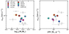 |
Fig. A.1. Outflow velocity vout as a function of host galaxy stellar stellar mass (M*, left panel) and star formation rate (SFR, right panel), for those SUPER AGN sources with available SED-based estimates or upper limits (Circosta et al. 2018). Errorbars on M* and SFR values represent the total uncertainty, including both statistical and typical systematic uncertainties (∼0.1dex in M* and 0.3dex in SFR, Pacifici et al. 2023). Colours and symbols are the same as in Figs. 8 and 10. The two panels show neither clear trend of vout with the host stellar properties nor separation between type-1 and type-2 measurements, which appear scattered together across the two planes. |
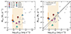 |
Fig. A.2. Outflow mass rates as a function of Lbol for the full SUPER sample. Upper and lower panels show our trust Ṁout values and Ṁmax mass rates, derived using vmax in Eq. 2. Triangles indicate lower limits to mass rates. In the lower panel, scaling relations from Fiore et al. (2017) and Musiimenta et al. (2023) are shown as dotted and dashed lines, after being re-scaled to ne = 500 adopted for our targets, while values of Ṁmax have been multiplied by a factor of 2 to match definitions adopted in Fiore et al. (2017) and Musiimenta et al. (2023). Compared to Fig. 8, the distribution of measurements is more scattered, with no clear discrepancy between the type-1 and type-2 samples. The comparison is furthermore hampered by the large number of lower limits to mass rates. |
All Tables
All Figures
|
Fig. 1. Integrated H- and K-band spectra extracted from SINFONI datacubes of XID36 (top), XID419 (middle), and XID614 (bottom), with a radius aperture of 0.25″, after subtracting continuum emission that was modelled with a first-degree polynomial. The data are shown in black, and the total emission-line model is overplotted in red. For multi-Gaussian modellings, we separately plot the narrow systemic (light blue) and broad high-velocity components (green) that are associated with outflows. In the top right panel, the solid and dashed green lines represent the outflow component of Hα and [N II] doublet, respectively. The mean velocity v and the velocity dispersion σ values of each Gaussian component are displayed. The shaded grey regions indicate masked channels that are contaminated by sky line residuals, and the vertical dotted lines mark the rest-frame emission line wavelengths at the redshift of each source, as computed in Sect. 3.1. Below each main panel, a second panel shows the corresponding residuals (i.e. data–model). |
| In the text | |
|
Fig. 2. Integrated H- and K-band spectra extracted from SINFONI datacubes of cid_1143 (top), cid_2682 (middle), and cid_451 (bottom), with a radius aperture of 0.25″, after subtracting continuum emission that was modelled with a first-degree polynomial. Same as in Fig. 2. In the K-band spectrum of cid_1143, we fit only the Hα line emission due to the low S/N (S/N < 2) of this dataset. |
| In the text | |
|
Fig. 3. Integrated H-band spectrum of cid_1057, extracted from a SINFONI datacube with a radius aperture of 0.25″, after subtracting continuum emission that was modelled with a first-degree polynomial. Same as in Fig. 2. Three Gaussian components are used to properly model the [O III] line profile: One component was used for the systemic narrow line emission (light blue), and two components were used for the blue and red wings detected in [O III] (different greens). |
| In the text | |
|
Fig. 4. Morphology and kinematics of ionised gas in XID36 and XID419 as traced by the total [O III] line emission. For each target, the maps show the intensity (moment-0) field; the v50, v10, and v90 percentile velocities and the w80 line width; and the ratio f300 of the flux contained in [O III] wings (i.e. |v|> 300 km s−1) to the moment-0 flux. The dashed and dotted circles correspond to the radius aperture of 0.25″ we used to extract the integrated spectra (Sect. 3.2) and to the mean H-band PSF with a radius of ⟨θPSF⟩/2, respectively (see Table 2). The two circles have the same 0.25″ radius in XID419. In all maps, we apply an S/N > 3 cut and mark the position of the [O III] peak emission with a cross. |
| In the text | |
|
Fig. 5. Morphology and kinematics of ionised gas in XID614 and cid_1143 as traced by the total [O III] line emission. Same as in Fig. 4. |
| In the text | |
|
Fig. 6. Morphology and kinematics of ionised gas in cid_2682 and cid_451 as traced by the total [O III] line emission. Same as in Fig. 4. |
| In the text | |
|
Fig. 7. Morphology and kinematics of ionised gas in cid_1057 as traced by the total [O III] line emission. Same as in Fig. 4. |
| In the text | |
|
Fig. 8. Outflow velocities vout and vmax (left and middle panels) as a function of Lbol, and vout/Lbol ratios vs. X-ray NH measurements (right panel). The coloured crosses and grey squares represent SUPER type-2 and type-1 AGN, and the triangles in the right panel indicate upper and lower limits to NH. The dash-dotted blue lines represent our best-fit linear relation to the type-1 measurements, from which the type-2 points depart increasingly at decreasing Lbol (the mean deviation is 0.4dex). In the middle panel, we draw the empirical relation by Fiore et al. (2017) for comparison (dotted line), along with a more recent version from Musiimenta et al. (2023) (dashed). The orange shading in the left and middle panels marks the low-Lbol range (i.e. Lbol = 1044.8 − 46.5 erg s−1), where we compare the type-1 and type-2 AGN measurements. In the right panel, we consistently use light orange markers to identify type-1 AGN in the low-Lbol regime. |
| In the text | |
|
Fig. 9. Stacked [O III]λ5007 spectra of type-2 (red) and type-1 (blue) AGN from SUPER with Lbol ∼ 1044.8 − 46.5 (orange shading in Fig. 8), resulting from integrated (aperture with a radius of 0.25″), subtracted [O III] spectra with S/N > 5. The integrated spectra were averaged by the inverse of the squared noise, and then the resulting stacked spectrum was normalised to the final [O III] peak. Comparing the two stacked spectra, we find a statistically significant (2.7σ) difference in the [O III] blue wing, which is more prominent in the type-2 spectrum of about 500 km s−1 compared to the type-1 stack. |
| In the text | |
|
Fig. 10. Outflow velocity vout as a function of escape velocity computed at Rout, as inferred from our mass modelling of SUPER type-2 (coloured symbols) and all those type-1 (grey) AGN galaxies with a known M*, hence not Lbol-matched to the type-2 AGN sample. We display two sets of escape speed values: One value was inferred according to the classical definition of the escape velocity to infinity (vout, left panel), hence, this needed to escape the DM halo (Rvir ∼ 80 − 160 kpc); the other value corresponded to the escape velocity required to reach 10 Re ( |
| In the text | |
|
Fig. 11. Same panels as in Fig. 8, showing SUPER type-2 (filled red circles) and type-1 (filled blue circles) measurements along with IFS-based results from the literature of other type-2 (empty red star; XID5395, Brusa et al. 2016) and type-1 AGN (empty blue symbols; Cano-Díaz et al. 2012; Carniani et al. 2015; Vayner et al. 2021a) at z ∼ 1 − 3. The orange symbols represent red obscured systems that were nevertheless optically classified as type-1 AGN (Perrotta et al. 2019; Vayner et al. 2021b; Cresci et al. 2023; Veilleux et al. 2023). Outflow velocities from Brusa et al. (2016) and Perrotta et al. (2019) have been corrected to account for discrepancies with the vout and vmax definitions we adopted (see Sect. 6). While the ‘standard’ blue type-1 and red type-2 from the literature agree with values found in SUPER, the orange points, almost all at Lbol ≳ 1047 erg s−1, clearly show that higher outflow velocities are recovered when we select optical type-1 but dusty obscured objects. |
| In the text | |
|
Fig. A.1. Outflow velocity vout as a function of host galaxy stellar stellar mass (M*, left panel) and star formation rate (SFR, right panel), for those SUPER AGN sources with available SED-based estimates or upper limits (Circosta et al. 2018). Errorbars on M* and SFR values represent the total uncertainty, including both statistical and typical systematic uncertainties (∼0.1dex in M* and 0.3dex in SFR, Pacifici et al. 2023). Colours and symbols are the same as in Figs. 8 and 10. The two panels show neither clear trend of vout with the host stellar properties nor separation between type-1 and type-2 measurements, which appear scattered together across the two planes. |
| In the text | |
|
Fig. A.2. Outflow mass rates as a function of Lbol for the full SUPER sample. Upper and lower panels show our trust Ṁout values and Ṁmax mass rates, derived using vmax in Eq. 2. Triangles indicate lower limits to mass rates. In the lower panel, scaling relations from Fiore et al. (2017) and Musiimenta et al. (2023) are shown as dotted and dashed lines, after being re-scaled to ne = 500 adopted for our targets, while values of Ṁmax have been multiplied by a factor of 2 to match definitions adopted in Fiore et al. (2017) and Musiimenta et al. (2023). Compared to Fig. 8, the distribution of measurements is more scattered, with no clear discrepancy between the type-1 and type-2 samples. The comparison is furthermore hampered by the large number of lower limits to mass rates. |
| In the text | |
Current usage metrics show cumulative count of Article Views (full-text article views including HTML views, PDF and ePub downloads, according to the available data) and Abstracts Views on Vision4Press platform.
Data correspond to usage on the plateform after 2015. The current usage metrics is available 48-96 hours after online publication and is updated daily on week days.
Initial download of the metrics may take a while.