| Issue |
A&A
Volume 690, October 2024
|
|
|---|---|---|
| Article Number | A238 | |
| Number of page(s) | 20 | |
| Section | Cosmology (including clusters of galaxies) | |
| DOI | https://doi.org/10.1051/0004-6361/202449513 | |
| Published online | 11 October 2024 | |
Cosmological constraints from the Planck cluster catalogue with new multi-wavelength mass calibration from Chandra and CFHT
1
Université Paris-Saclay, CNRS, Institut d’Astrophysique Spatiale,
91405
Orsay,
France
2
Université Paris-Saclay, Université Paris Cité, CEA, CNRS, AIM,
91191
Gif-sur-Yvette,
France
3
Center for Astrophysics | Harvard & Smithsonian,
Cambridge,
MA
02138,
USA
4
Department of Liberal Arts and Sciences, Berklee College of Music,
7 Haviland Street,
Boston,
MA
02215,
USA
5
Leiden Observatory, Leiden University,
PO Box 9513,
2300 RA
Leiden,
The Netherlands
★ Corresponding author; This email address is being protected from spambots. You need JavaScript enabled to view it.
Received:
6
February
2024
Accepted:
19
August
2024
Abstract
We provide a new scaling relation between YSZ, the integrated Sunyaev-Zeldovich signal and M500YX, the cluster mass derived from X-ray observations, using a sample of clusters from the Planck Early Sunyaev-Zeldovich (ESZ) catalogue observed in X-rays by Chandra, and compare it to the results of the Planck collaboration obtained from XMM-Newton observations of a subsample of the ESZ. We calibrated a mass bias on a subset of the Planck cosmological cluster sample using published weak-lensing data from the Canadian Cluster Cosmology Project (CCCP) and Multi Epoch Nearby Cluster Survey (MENeaCS), for the new scaling relation as well as that from the Planck collaboration. We propose a novel method to account for selection effects and find a mass bias of (1 − b) = 0.89 ± 0.04 for the Chandra-calibrated scaling relation, and (1 − b) = 0.76 ± 0.04 for the XMM-Newton-calibrated scaling relation. We applied the scaling relations we derived to the full Planck cosmological cluster sample and obtain new constraints on the cosmological parameters. We find identical constraints regardless of the X-ray sample used, with σ8 = 0.77 ± 0.02, Ωm = 0.31 ± 0.02, and S8 ≡ σ8 √(Ωm/0.3) = 0.78 ± 0.02. We also provide constraints with a redshift evolution of the scaling relation fitted from the data instead of fixing it to the self-similar value. We find a redshift evolution significantly deviating from the self-similar value, leading to a higher value of S8 = 0.81 ± 0.02. We compare our results to those from various cosmological probes, and find that our S8 constraints are competitive with the tightest constraints from the literature. When assuming a self-similar redshift evolution, our constraints are in agreement with most late-time probes and in tension with constraints from the cosmic microwave background (CMB) primary anisotropies. When relaxing the assumption of redshift evolution and fitting it to the data, we find no significant tension with results from either late-time probes or the CMB.
Key words: galaxies: clusters: general / cosmological parameters / cosmology: observations / large-scale structure of Universe / X-rays: galaxies: clusters
© The Authors 2024
 Open Access article, published by EDP Sciences, under the terms of the Creative Commons Attribution License (https://creativecommons.org/licenses/by/4.0), which permits unrestricted use, distribution, and reproduction in any medium, provided the original work is properly cited.
This article is published in open access under the Subscribe to Open model. This email address is being protected from spambots. You need JavaScript enabled to view it. to support open access publication.
1 Introduction
In the hierarchical structure formation scenario, galaxy clusters emerge from peaks in the initial density field and grow through accretion and mergers, due to the depth of their gravitational potential wells (Kravtsov & Borgani 2012). Galaxy clusters are therefore tracers of the formation of cosmic structures throughout the evolution of the Universe and can be used to constrain the parameters of the cosmological model (White et al. 1993; Henry 1997; Allen et al. 2011). In particular, the abundance of clusters as a function of redshift and mass is closely related to the matter density Ωm and the amplitude of density fluctuations σ8, and to the dark energy equation of state when considering extensions to the standard Λ-Cold Dark Matter (ΛCDM) cosmological model. Galaxy clusters are thus a powerful cosmological probe, and their abundance has been used to constrain cosmological parameters in numerous studies (e.g. Vikhlinin et al. 2009b; Rozo et al. 2010; Planck Collaboration XX 2014; Bocquet et al. 2019; Costanzi et al. 2021; Garrel et al. 2022; Lesci et al. 2022; Bocquet et al. 2024; Ghirardini et al. 2024).
A key feature of galaxy clusters is their multi-component nature: they are composed of a dark matter halo, which is the main component of their mass, and of baryonic matter in the form of both hot gas and galaxies. They can therefore be observed through multiple physical processes depending on the wavelength, revealing different properties of the cluster. In optical wavelengths, the member galaxies can be directly observed, and the cluster can also be detected through the gravitational lensing effect on background galaxies. In X-rays, the hot gas emits thermal bremsstrahlung radiation, and in the microwave wavelengths, the hot gas interacts with the cosmic microwave background (CMB) photons through the thermal Sunyaev-Zel’dovich (SZ) effect (Sunyaev & Zeldovich 1972).
SZ surveys are a choice candidate for cluster cosmology since CMB experiments provide wide-field cluster surveys at no additional observational cost. Additionally, the SZ signal is independent of the cluster redshift, allowing for detections up to z~2 with the most recent surveys. Recently, SZ cluster catalogues have been obtained from the Planck satellite (Planck Collaboration XXIX 2014; Planck Collaboration XXVII 2016), the South Pole Telescope (Bleem et al. 2015, 2020; Klein et al. 2024; Bleem et al. 2024), and the Atacama Cosmology Telescope (Hilton et al. 2021).
In order to compare cluster abundance observations with theoretical predictions, it is necessary to know the cluster mass, which is the fundamental quantity in the theory of structure formation (Pratt et al. 2019). While the SZ effect allows for the construction of large cluster catalogues, it does not provide a direct measurement of the cluster mass, as the observed quantity is the integrated SZ signal, noted YSZ in this work, which is proportional to the gas pressure integrated along the line of sight. To use SZ surveys as a cosmological probe, it is thus necessary to relate the SZ signal to the cluster mass, usually via a scaling relation calibrated using a sub-sample of clusters from the SZ catalogue for which other observations allow for mass estimations. This mass calibration step is critical, as it is the main source of uncertainty and systematic error in the cosmological constraints obtained from SZ surveys. An example of the importance of mass calibration is found in Planck Collaboration XXIV (2016), where constraints were obtained from the same SZ catalogue using three different mass calibrations varying by up to ~30%, from Weighing the Giants (Von Der Linden et al. 2014), the Canadian Cluster Comparison Project (CCCP) (Hoekstra et al. 2015), and CMB lensing (calibration performed by the Planck collaboration, using the method presented in Melin & Bartlett 2015), yielding σ8 (Ωm/0.31)0.3 values differing by more than 2σ, and tensions with the value obtained from the analysis of the primary anisotropies of the CMB ranging from nearly full agreement to ~2σ.
Mass estimates can be obtained from X-ray observations that provide precise gas density and temperature profiles, from which masses can be calculated under the hydrostatic equilibrium hypothesis, that is, assuming that the gas contained in the cluster is at equilibrium, with the thermal pressure balancing the gravitational potential. Mass estimates from X-ray observations have low statistical uncertainties but are subject to systematic errors. These errors can be due to the presence of non-thermal pressure, coming from magnetic fields (e.g. Dolag & Schindler 2000), cosmic rays (e.g. Böss et al. 2022), or turbulence (e.g. Rasia et al. 2004; Pearce et al. 2020; Gianfagna et al. 2021). Another source of error in mass determination is the dynamical state and local environment of the cluster (Gouin et al. 2021, 2022). Complex temperature structures in the intracluster medium can also affect the mass calculated from X-ray observations (Rasia et al. 2006).
The mass of a cluster can also be estimated through the gravitational lensing effect, which does not require assumptions on the dynamical state of the cluster, but usually suffers from large statistical uncertainties due to the long exposure times required to get a sufficient number of background galaxies.
In the Planck collaboration 2013 and 2015 papers (Planck Collaboration XX 2014; Planck Collaboration XXIV 2016), cosmological parameters were constrained using the number counts of SZ-detected clusters. In this work, our aim is to improve on the Planck collaboration approach by focusing on the mass calibration step. We leverage a larger, SZ-selected X-ray calibration sample from the Chandra-Planck Legacy Program as well as a larger weak-lensing sample from Herbonnet et al. (2020) using data from the Canadian Cluster Comparison Project (CCCP) and the Multi Epoch Nearby Cluster Survey (MENeaCS) to provide a new mass calibration and cosmological constraints.
In addition to the improved statistical power, our results provide a robustness check regarding potential instrumental systematics to the constraints formerly obtained, as the Planck X-ray calibration sample was obtained from XMM-Newton data, whereas the new calibration sample was obtained from Chandra observations of Planck-detected clusters. Given that the two instruments are known to yield different results (see Schellenberger et al. 2015; Potter et al. 2023), evaluating the effect of instrumental differences on the final constraints is crucial to understanding the reliability of our results.
The paper is organised as follows: in Sec. 2, we present the data sets used in this work, and in Sec. 3, we calibrate the YSZ − M500 scaling relation using the Chandra-Planck sample. In Sec. 4, we constrain the cosmological parameters using the Planck cosmological cluster sample and the scaling relation calibrated in Sec. 3, and compare our results with the ones obtained by the Planck collaboration. In Sec. 5, we discuss the possible systematics impacting our cosmological constraints, explore the impact of fitting the redshift dependence of the scaling relation instead of fixing it to the self-similar value, and compare our results to the ones from recent analyses based on various cosmological probes. Finally, in Sect. 6, we summarise our results and conclude.
For this work, we use the following reference cosmology: Ωm = 0.3, ΩΛ = 0.7, H0 = 70 km s−1 Mpc−1. Unless explicitly stated, all quantities are given within R500, the radius within which the mean density is 500 times the critical density of the Universe at the cluster redshift.
2 Data and analysis
2.1 Chandra observation of Planck ESZ sample
For our investigation, we use the data set from the Chandra-Planck Legacy Program for Massive Clusters of Galaxies1, which is a full follow-up observation with the Chandra X-ray observatory of the 163 clusters with redshift z <0.35 from the Planck ESZ catalogue, which is constructed from clusters detected with a signal-to-noise ratio above 6 in the Planck early results maps (Planck Collaboration VIII 2011). All 163 clusters were observed with sufficient exposures to obtain a minimum of 10000 source counts. Six clusters that fall outside the more restrictive mask used to obtain the Planck PSZ2 cosmological catalogue (Planck Collaboration XXVII 2016) were discarded from the analysis: PLCKESZ G115.71+17.52, G228.49+53.12, G269.51+26.42, G275.21+43.92, G282.49+65.17, G315.70-18.04. Nine clusters were identified as multiple systems in the X-ray data, and were also discarded as the size of the Planck beam did not allow for proper disentanglement of the two components in the SZ data: PLCKESZ G039.85-39.98, G062.42-46.41, G107.11+65.31, G124.21-36.48, G195.62+44.05, G241.85+51.53, G263.20-25.21, G337.09-25.97, G345.40-39.34. Finally, we removed PLCKESZ G234.59+73.01 (A1367/Leo cluster at z = 0.02) and PLCKESZ G057.33+88.01 (A1656/Coma cluster at z = 0.02), two nearby clusters whose size did not allow for a proper data reduction. The final sample thus contains 146 clusters with high-quality data in both X-ray and SZ, allowing for a multi-wavelength analysis and robust calibration of the YSZ − M500 scaling relation.
The sample and X-ray data reduction process is fully described in Andrade-Santos et al. (2021) (see also Vikhlinin et al. 2005), and we refer the reader to these papers for more details. A summary of the data reduction process is given in Sec. 2.4.
Fig. 1 shows the redshift and mass distribution of the sample used in this work, and compares it to the Planck PSZ2 cosmological sample and the X-ray calibration sample used in Planck Collaboration XX (2014) and Planck Collaboration XXVII (2016).
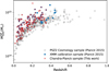 |
Fig. 1 Mass-redshift distribution of the Chandra-Planck sample, the Planck MMF3 cosmological sample, and the XMM-Newton calibration sample used by the Planck collaboration. |
2.2 Data sets of the Planck collaboration
The Planck PSZ2 cosmological sample, presented in Planck Collaboration XXVII (2016), is composed of all the clusters detected in Planck HFI maps by the matched multi-frequency filter algorithm MMF3 (Melin et al. 2006) with a signal-to-noise ratio above 6. The detection procedure uses a more restrictive mask of contaminated regions than the full PSZ2 catalogue, leaving only 65% of the sky unmasked, to ensure a very high purity of the sample. It contains 439 clusters and is the sample used to constrain cosmological parameters via MCMC fitting of the number counts in Planck Collaboration XXIV (2016). To estimate the masses of the clusters, the Planck collaboration used a scaling relation between the SZ signal and the cluster mass, calibrated on a sub-sample of 71 clusters with X-ray observations from XMM-Newton Planck Collaboration XX (2014). In this work, we use a new calibration sample of 146 clusters from the Planck ESZ catalogue with Chandra X-ray observations.
Compared to the XMM-Newton sample, the Chandra calibration sample has more clusters and extends to lower masses and redshifts. Given the cut at redshift 0.35, the maximum redshift of the Chandra sample is lower than the one of the XMM-Newton sample, which has six clusters with 0.35 < z < 0.45.
Beyond the mass and redshift ranges, the most important difference between the two calibration samples is the selection of the sample. As a full X-ray follow-up of the Planck ESZ sample, the Chandra sample is SZ-selected (with the additional removal of the nine multiple systems and two nearby clusters) and therefore is subject to the same type of selection biases as the clusters in the Planck catalogues. The XMM-Newton sample, on the other hand, is a subset of 71 detections from the Planck cosmological cluster sample, detected at signal-to-noise ratio above 7, for which good quality XMM-Newton observations were available (Planck Collaboration XX 2014). The XMM-Newton sample is therefore not guaranteed to be representative of the Planck cosmological sample and is likely to be biased towards X-ray bright clusters. Since the selection function of the X-ray sample is not known, it was not possible to correct for this bias in Planck Collaboration XX (2014). This issue of the representativity of the calibration sample is investigated in depth in Appendix D.
2.3 Weak lensing data: CCCP and MENeaCS samples
In this work, we use the results of Herbonnet et al. (2020) who derived masses for 100 clusters from the Canadian Cluster Comparison Project (CCCP) and the Multi Epoch Nearby Cluster Survey (MENeaCS). It currently is one of the largest coherent weak-lensing cluster samples, combining two data sets coming from observations with the Canada-France-Hawaii Telescope (CFHT) with similar depth, and analysing them with the same pipeline. A detailed description of the CCCP sample is available in Hoekstra et al. (2012) and Sand et al. (2011, 2012) provide a full description of the MENeaCS sample. Both data sets are X-ray-selected cluster samples, with MENeaCS containing 48 low redshift clusters with 0.05 < z < 0.15 and CCCP containing 52 higher redshift clusters with 0.15 < z < 0.55. The analysis procedure used to derive the masses from the optical imaging surveys is described in Herbonnet et al. (2020).
2.4 X-ray data reduction and mass estimates
The full data reduction process from raw event files to profiles is described in Andrade-Santos et al. (2021). In this section, we briefly summarise the main steps of the data reduction process.
Charge-transfer inefficiency, mirror contamination, CCD non-uniformity, and time dependence of gain are corrected for during data reduction. High background periods are removed, and blank sky background and readout artefacts are subtracted from the signal. Point sources and extended substructures are masked before analysing the cluster emission.
Surface brightness profiles are extracted in the 0.7–2 keV band, where the signal-to-noise ratio is maximal, in concentric annuli around the X-ray emission peak. Spectra are extracted in larger concentric annuli, and fitted with an absorbed single-temperature thermal model. The projected temperature profiles are then fitted with a 3D temperature model to obtain the deprojected temperature profiles. These are then used to compute the emission measure profiles from the surface brightness, which are fitted with the gas density model given by Vikhlinin et al. (2006).
In Andrade-Santos et al. (2021), total cluster masses are computed from the gas mass and temperature, using the YX − M500 scaling relation calibrated in Vikhlinin et al. (2009a):
![Mathematical equation: $\[M_{500}=E(z)^{-2 / 5} A_{\mathrm{YM}}\left(\frac{Y_{\mathrm{X}}}{3 \cdot 10^{14} ~M_{\mathrm{\odot}} \mathrm{keV}}\right)^{B_{\mathrm{YM}}},\]$](/articles/aa/full_html/2024/10/aa49513-24/aa49513-24-eq3.png) (1)
(1)
where ![Mathematical equation: $\[A_{\mathrm{YM}}=(5.77 \pm 0.20) \cdot 10^{14} h^{1 / 2} M_{\odot}, B_{\mathrm{YM}}=0.57 \pm 0.03\]$](/articles/aa/full_html/2024/10/aa49513-24/aa49513-24-eq4.png) , and
, and ![Mathematical equation: $\[E(z)=\sqrt{\Omega_{m}(1+z)^{3}+\Omega_{\Lambda}}\]$](/articles/aa/full_html/2024/10/aa49513-24/aa49513-24-eq5.png) .
.
The quantity ![Mathematical equation: $\[Y_{\mathrm{X}}=M_{\text {gas }} T_{\mathrm{X}}^{\text {exc }}\]$](/articles/aa/full_html/2024/10/aa49513-24/aa49513-24-eq6.png) is defined in Kravtsov et al. (2006) as the product of Mgas, the gas mass inside R500, and
is defined in Kravtsov et al. (2006) as the product of Mgas, the gas mass inside R500, and ![Mathematical equation: $\[T_{\mathrm{X}}^{\text {exc }}\]$](/articles/aa/full_html/2024/10/aa49513-24/aa49513-24-eq7.png) , the core-excised temperature obtained by fitting a single temperature MEKAL model to the spectral data in the 0.15 R500–R500 region. It is thus measured within R500, and the mass calculations have to be done following an iterative process. A first mass estimate is computed from the TX − M500 scaling relation, giving a first R500 value. The YX value is then computed within this first R500, which gives a new mass estimate, leading to new R500 and YX values, and so on until convergence. At each step, to calculate
, the core-excised temperature obtained by fitting a single temperature MEKAL model to the spectral data in the 0.15 R500–R500 region. It is thus measured within R500, and the mass calculations have to be done following an iterative process. A first mass estimate is computed from the TX − M500 scaling relation, giving a first R500 value. The YX value is then computed within this first R500, which gives a new mass estimate, leading to new R500 and YX values, and so on until convergence. At each step, to calculate ![Mathematical equation: $\[Y_{\mathrm{X}}, T_{\mathrm{X}}^{\text {exc }}\]$](/articles/aa/full_html/2024/10/aa49513-24/aa49513-24-eq8.png) is re-extracted in the new 0.15 R500–R500 region.
is re-extracted in the new 0.15 R500–R500 region.
A possible caveat of the approach is that the Vikhlinin et al. (2009a) scaling relation was derived for an X-ray-selected sample, whereas the sample discussed in this work is SZ-selected. However, there is currently no strong evidence that the YX − M500 scaling relations recovered from X-ray and SZ-selected samples differ. Theoretically, the original motivation for YX was that it is a quantity that is independent of selection and/or dynamical state (as is detailed in Kravtsov et al. 2006). Observationally, Fig. 8 of Andrade-Santos et al. (2021) compares the YSZ − YX relations for an SZ- and an X-ray selected sample. There clearly is no evidence for any difference between the SZ and the X-ray-selected systems. We therefore assume that the scaling relation of Eq. (1) is valid for our sample.
2.5 SZ signal extraction from Planck data
As shown in Planck Collaboration XI (2011), using an external prior on the size and position can lead to more robust SZ flux estimates, given the size of the Planck beam (around 7 arcmin). To calibrate the YSZ − M500 scaling relation, we use the SZ signal extracted from the Planck DR2 maps, by running a matched multi-frequency filter algorithm (Herranz et al. 2002), with the X-ray derived positions and sizes as prior information. We use the Planck DR2 maps, even though newer maps are available as this work uses the PSZ2 cosmological sample obtained on DR2 maps. While deriving a new catalogue from the most recent Planck data would be possible and possibly beneficial in terms of final cosmological constraints, it would introduce an unnecessary inconsistency in the comparison of mass calibration samples between this work and the original Planck 2015 analysis. The MMF algorithm extracts the YSZ signal from the six Planck HFI maps (100, 143, 217, 353, 545, and 857 GHz) using the SZ frequency spectrum and the universal pressure profile from Arnaud et al. (2010), scaled to an aperture θ500 corresponding to ![Mathematical equation: $\[R_{500}^{\mathrm{X} \text {-ray }}\]$](/articles/aa/full_html/2024/10/aa49513-24/aa49513-24-eq9.png) , convolved with the instrumental beam as a template. The extraction is performed on a 10°×10° patch centred on the X-ray cluster position, with a pixel size of 1.72×1.72 arcmin2. The signal is integrated up to 5R500, then scaled back to R500, using the assumed pressure profile. The noise auto- and cross-spectra are directly calculated from the data. This python MMF implementation uses the same approach and steps as the IDL MMF3 implementation used in Planck Collaboration XXVII (2016). We refer the reader to that paper, and references therein, for more details.
, convolved with the instrumental beam as a template. The extraction is performed on a 10°×10° patch centred on the X-ray cluster position, with a pixel size of 1.72×1.72 arcmin2. The signal is integrated up to 5R500, then scaled back to R500, using the assumed pressure profile. The noise auto- and cross-spectra are directly calculated from the data. This python MMF implementation uses the same approach and steps as the IDL MMF3 implementation used in Planck Collaboration XXVII (2016). We refer the reader to that paper, and references therein, for more details.
This extraction step was done both in Andrade-Santos et al. (2021) and in this work, using the same X-ray input positions and aperture, but fully independently developed MMF algorithms. Appendix E shows the excellent agreement between the results.
3 YSZ − M500 scaling relation
Relating the SZ signal to the cluster mass is required to compare the cluster number counts with theoretical predictions and constrain the underlying cosmological parameters. In this section we calibrate a YSZ − M500 scaling relation, using the Chandra calibration sample described in Sec. 2, for which we have both SZ measurements and mass estimates from the X-ray observations. We also use the weak-lensing masses derived in Herbonnet et al. (2020) as a true mass anchor to calibrate the hydrostatic mass bias.
3.1 Calibrating the scaling relation
To study the effect of changing the calibration sample, we calibrate the YSZ − M500 scaling relation following the Planck collaboration approach described in Appendix A of Planck Collaboration XX (2014). Since the ESZ sample is signal-to-noise limited, the detected objects are biased high with respect to the mean close to the signal-to-noise threshold, due to the intrinsic scatter of the relation. This effect, commonly known as Malmquist bias, needs to be corrected to retrieve the underlying scaling relation in an unbiased way. We follow the same approach as in Planck Collaboration XX (2014), which is based on the method presented in Vikhlinin et al. (2009a), to account for Malmquist bias. The detailed justification of the method can be found in Appendix A.2 of Vikhlinin et al. (2009a), simply replacing luminosity with YSZ and the flux cut with a signal-to-noise cut. Each individual YSZ value is corrected by dividing it by the mean bias m at the corresponding signal-to-noise ratio, assuming a log-normal intrinsic scatter σint:
![Mathematical equation: $\[Y_{\mathrm{SZ}}^{\text {corrected }}=Y_{\mathrm{SZ}} / m \text { with } \ln m=\frac{\exp \left(-x^2 / 2 \sigma^2\right)}{\sqrt{\pi / 2} \operatorname{erfc}(-x / \sqrt{2} \sigma)} \sigma \text {, }\]$](/articles/aa/full_html/2024/10/aa49513-24/aa49513-24-eq10.png) (2)
(2)
where (S /N)cut is the signal-to-noise threshold of the sample, ![Mathematical equation: $\[x=\]$](/articles/aa/full_html/2024/10/aa49513-24/aa49513-24-eq11.png)
![Mathematical equation: $\[-\log \left(\frac{(S / N)}{(S / N)_{\text {cut }}}\right)\]$](/articles/aa/full_html/2024/10/aa49513-24/aa49513-24-eq12.png) , and
, and ![Mathematical equation: $\[\sigma=\sqrt{\ln [((S / N)+1) /(S / N)]^{2}+\left(\ln 10 \sigma_{\text {int }}\right)^{2}}\]$](/articles/aa/full_html/2024/10/aa49513-24/aa49513-24-eq13.png)
The corrected YSZ values are then used to calibrate the ![Mathematical equation: $\[Y_{\mathrm{SZ}}-M_{500}^{Y_{\mathrm{X}}}\]$](/articles/aa/full_html/2024/10/aa49513-24/aa49513-24-eq14.png) scaling relation, assuming the following form for the relation:
scaling relation, assuming the following form for the relation:
![Mathematical equation: $\[E^{-2 / 3}(z) \frac{D_A^2 Y_{\mathrm{SZ}}}{Y_{\mathrm{piv}}}=10^{Y^*}\left(\frac{M_{500}^{Y_{\mathrm{X}}}}{M_{\mathrm{piv}}}\right)^\alpha.\]$](/articles/aa/full_html/2024/10/aa49513-24/aa49513-24-eq15.png) (3)
(3)
To allow for easy comparison, the pivot points were chosen to be the same in this work as in Planck Collaboration XX (2014), that is, Mpiv = 6 · 1014 M⊙ and Ypiv = 10−4Mpc2. We fit the data via a Markov chain Monte Carlo (MCMC) approach with the emcee sampler, using a standard Gaussian log-likelihood with intrinsic scatter:
![Mathematical equation: $\[\ln \mathcal{L}=-0.5 {\sum}_{i=1}^N\left[\frac{\left(y_i-\left(\alpha x_i+10^{Y^*}\right)\right)^2}{2 \sigma_i^2}-\ln \left(\frac{1+10^{2 Y^*}}{2 \pi \sigma_i^2}\right)\right],\]$](/articles/aa/full_html/2024/10/aa49513-24/aa49513-24-eq16.png) (4)
(4)
where xi and yi are the logarithm of the mass and YSZ values of the ith cluster, ![Mathematical equation: $\[\sigma_{x_{i}}\]$](/articles/aa/full_html/2024/10/aa49513-24/aa49513-24-eq17.png) and
and ![Mathematical equation: $\[\sigma_{y_{i}}\]$](/articles/aa/full_html/2024/10/aa49513-24/aa49513-24-eq18.png) are the uncertainties on the mass and YSZ values, σint is the intrinsic scatter of the relation, and
are the uncertainties on the mass and YSZ values, σint is the intrinsic scatter of the relation, and ![Mathematical equation: $\[\sigma_{i}^{2}=\sigma_{\text {int }}^{2}+10^{2 Y^{*}} \sigma_{x_{i}}^{2}+\sigma_{y_{i}}^{2}\]$](/articles/aa/full_html/2024/10/aa49513-24/aa49513-24-eq19.png) .
.
The varying parameters are the normalisation Y*, the slope α, and the intrinsic scatter σint. The only prior is requiring the intrinsic scatter to be positive. Since the intrinsic scatter is not known a priori and is required to calculate the Malmquist bias correction, this fitting procedure is an iterative process, where the intrinsic scatter used to compute the mean bias is updated at each step to the value obtained once the relation is fitted. Since the Malmquist bias correction is negligible for most clusters, the convergence is reached after only 4 to 5 steps.
Two other linear regression methods were tried: LinMix (Kelly 2007) and BCES (Akritas & Bershady 1996), with no significant difference in the results. We thus only report the results obtained with the MCMC method using the emcee sampler in the rest of this work. Fig. 2 shows the scaling relation obtained with the emcee sampler, and compares it with the one obtained by the Planck collaboration with the XXMM-Newton calibration sample.
This scaling relation is not final: the ![Mathematical equation: $\[Y_{\mathrm{SZ}}-M_{500}^{Y_{\mathrm{X}}}\]$](/articles/aa/full_html/2024/10/aa49513-24/aa49513-24-eq20.png) relation needs to be combined with the
relation needs to be combined with the ![Mathematical equation: $\[M_{500}^{Y_{\mathrm{X}}}-M_{500}\]$](/articles/aa/full_html/2024/10/aa49513-24/aa49513-24-eq21.png) relation to obtain the YSZ − M500 relation. The
relation to obtain the YSZ − M500 relation. The ![Mathematical equation: $\[M_{500}^{Y_{\mathrm{X}}}-M_{500}\]$](/articles/aa/full_html/2024/10/aa49513-24/aa49513-24-eq22.png) relation has the following form, with σA and σα the uncertainties in the normalisation and slope of the YX − M500 relation taken from Vikhlinin et al. (2009a):
relation has the following form, with σA and σα the uncertainties in the normalisation and slope of the YX − M500 relation taken from Vikhlinin et al. (2009a):
![Mathematical equation: $\[M_{500}^{Y_{\mathrm{X}}}=10^{ \pm \sigma_A / \alpha}\left[(1-b) M_{500}\right]^{1 \pm \sigma_\alpha / \alpha}.\]$](/articles/aa/full_html/2024/10/aa49513-24/aa49513-24-eq23.png) (5)
(5)
Combining the ![Mathematical equation: $\[Y_{\mathrm{SZ}}-M_{500}^{Y_{\mathrm{X}}}\]$](/articles/aa/full_html/2024/10/aa49513-24/aa49513-24-eq25.png) and
and ![Mathematical equation: $\[M_{500}^{Y_{\mathrm{X}}}-M_{500}\]$](/articles/aa/full_html/2024/10/aa49513-24/aa49513-24-eq26.png) relations, we obtain the following YSZ − M500 relation:
relations, we obtain the following YSZ − M500 relation:
![Mathematical equation: $\[E^{-2 / 3}(z) \frac{D_A^2 ~Y_{\mathrm{SZ}}}{Y_{\text {piv }}}=10^{-0.29 \pm 0.01}\left(\frac{(1-b) M_{500}}{M_{\text {piv }}}\right)^{1.70 \pm 0.1}.\]$](/articles/aa/full_html/2024/10/aa49513-24/aa49513-24-eq27.png) (6)
(6)
Moving from ![Mathematical equation: $\[Y_{\mathrm{SZ}}-M_{500}^{Y_{\mathrm{X}}}\]$](/articles/aa/full_html/2024/10/aa49513-24/aa49513-24-eq28.png) to
to ![Mathematical equation: $\[Y_{\mathrm{SZ}}-M_{500}\]$](/articles/aa/full_html/2024/10/aa49513-24/aa49513-24-eq29.png) , the best-fit parameters do not change, but the uncertainties of the
, the best-fit parameters do not change, but the uncertainties of the ![Mathematical equation: $\[M_{500}^{Y_{X}}-M_{500}\]$](/articles/aa/full_html/2024/10/aa49513-24/aa49513-24-eq30.png) relation are propagated, leading to increased uncertainties in the final YSZ − M500 relation, by ~2 for the slope and ~1.3 for the normalisation. In addition, the scatter around the mean relation is also affected: assuming the scatter around both relations is independent, our final estimate of the scatter is
relation are propagated, leading to increased uncertainties in the final YSZ − M500 relation, by ~2 for the slope and ~1.3 for the normalisation. In addition, the scatter around the mean relation is also affected: assuming the scatter around both relations is independent, our final estimate of the scatter is ![Mathematical equation: $\[\sigma_{Y_{\mathrm{SZ}}-M_{500}}=21 \%\]$](/articles/aa/full_html/2024/10/aa49513-24/aa49513-24-eq31.png) .
.
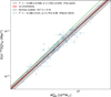 |
Fig. 2 Calibration of the |
![Mathematical equation: $\[Y_{\mathrm{SZ}}-M_{500}^{Y_{\mathrm{X}}}\]$](/articles/aa/full_html/2024/10/aa49513-24/aa49513-24-eq24.png)
3.2 Hydrostatic mass bias
In the previous section, we calibrated the scaling relation between the SZ signal and the cluster mass. However, the masses used for calibration were obtained from X-ray observations and are not the true masses of the clusters, but biased estimates, since their calculation indirectly relies on the hypothesis of hydrostatic equilibrium, through the YX − M500 relation. This is usually referred to as the hydrostatic mass bias and is accounted for by a multiplicative factor (1 − b) in the scaling relation 6. This free parameter needs to be constrained using an independent, ideally bias-free, mass estimate of the clusters, before using the scaling relation to constrain cosmological parameters. In this work, we follow the approach of Planck Collaboration XXIV (2016) to use an external weak-lensing data set to constrain the bias. Similarly to Planck Collaboration XXIV (2016), we consider a constant bias, but some studies have investigated a potential dependence of the bias on the cluster mass and redshift (e.g. Salvati et al. 2019; Wicker et al. 2023). In this work, we use weak-lensing masses obtained in Herbonnet et al. (2020) to constrain the value of (1 − b). This data set was already used to provide tight constraints on the hydrostatic mass bias in Herbonnet et al. (2020). They compared the weak-lensing mass estimates with SZ masses derived from Planck data for the 61 clusters in their data set that were detected by Planck, and found a bias of (1 − b) = 0.84 ± 0.04.
However, this bias value cannot be directly used in this work, since it was obtained by comparing the weak-lensing masses with the Planck SZ-derived masses calculated using the scaling relation calibrated in Planck Collaboration XX (2014) using XMM-Newton X-ray data. The value of the bias thus needs to be re-estimated using the new scaling relation calibrated in this work.
Battaglia et al. (2016) showed that selection effects can lead to overestimating the mass bias, with an expected effect between 3–15%. Here, we propose a method to account for this effect, based on the idea proposed in Battaglia et al. (2016) to treat the Planck measurements as follow-up observations of the weak-lensing sample. When approaching the problem under this angle, a cluster from the weak-lensing sample not detected by Planck is a source of information, since the Planck catalogue is signal-to-noise-limited.
The first step is to remove the clusters of the weak-lensing sample that lie in the masked region of the Planck data, since they will necessarily not be detected by Planck, and will not provide any information. We find 8 clusters (A780, A1285, A2050, ZWCL1023, ZWCL1215, A2104, A2163, MS0440) in the mask used for the extraction of the PSZ2 cosmological catalogue, and remove them from the sample, after manually verifying their absence from the cosmological sample. This leaves 92 clusters in the weak-lensing sample that can potentially have a match in the Planck catalogue. We also remove 5 clusters that are part of multiple systems detected as a single source by Planck: A115N, A115S, A223N, A223S, and A119 (not removed in Herbonnet et al. 2020). We then match the remaining clusters with the full Planck PSZ2 cosmological catalogue and find 56 direct matches, as opposed to 61 in Herbonnet et al. (2020) (60 matches when excluding A119). Since the list of matches is not available in Herbonnet et al. (2020), our best guess is that the difference can be explained by the mask used, since they only remove 1 out of 100 clusters before matching due to lying in the Planck mask, while we find 8 clusters in the mask.
We then calculate the Planck mass of the matched clusters with the YSZ − M500 scaling relation calibrated in this work:
![Mathematical equation: $\[M_{500}^{\mathrm{SZ}}=M_{\mathrm{piv}}\left(10^{-Y^*} E^{-2 / 3}(z) \frac{D_A^2 ~Y_{\mathrm{SZ}}}{Y_{\mathrm{piv}}}\right)^{\frac{1}{\alpha}}.\]$](/articles/aa/full_html/2024/10/aa49513-24/aa49513-24-eq32.png) (7)
(7)
To break the size-flux degeneracy, we need to combine it with the θ500 − M500 relation (see Planck Collaboration XXVII 2016). We use an MCMC approach to compute the masses, allowing for proper marginalisation over both the posterior probability distribution in the YSZ − θSZ plane given in the Planck catalogue and the uncertainties of the scaling relation parameters (see Appendix A).
If no match is found, we compute the upper limit of the Planck mass given the S/N = 6 detection threshold of the Planck cosmological catalogue, using the noise level N of the Planck map at the cluster position, for the aperture θ500 corresponding to ![Mathematical equation: $\[R_{500}^{\mathrm{WL}}\]$](/articles/aa/full_html/2024/10/aa49513-24/aa49513-24-eq33.png) :
:
![Mathematical equation: $\[M_{500}^{S Z, \lim }=M_{\text {piv }}\left(10^{-Y^*} E^{-2 / 3}(z) \frac{D_A^2 ~6 N}{Y_{\text {piv }}}\right)^{\frac{1}{\alpha}}.\]$](/articles/aa/full_html/2024/10/aa49513-24/aa49513-24-eq34.png) (8)
(8)
The choice of the WL aperture is an approximation, but it is justified by the shallow dependence of the noise level on the aperture and the fact that θ500 scales as ![Mathematical equation: $\[M_{500}^{1 / 3}\]$](/articles/aa/full_html/2024/10/aa49513-24/aa49513-24-eq35.png) .
.
We then use a modified version of the MCMC power-law regression algorithm detailed in Sect. 3 on the ![Mathematical equation: $\[M_{500}^{\mathrm{SZ}}-M_{500}^{\mathrm{WL}}\]$](/articles/aa/full_html/2024/10/aa49513-24/aa49513-24-eq36.png) data, with the slope set to unity, to find the best-fit normalisation value, which corresponds to the best fit hydrostatic mas bias value (1 − b). The likelihood is the same as in Eq. (4) with α set to 1, and the addition of the method detailed below to deal with non-detections. For non-detected clusters, at each step of the MCMC algorithm, we draw a mass from a log-normal distribution, with the current model value at the WL mass as mean and standard deviation
data, with the slope set to unity, to find the best-fit normalisation value, which corresponds to the best fit hydrostatic mas bias value (1 − b). The likelihood is the same as in Eq. (4) with α set to 1, and the addition of the method detailed below to deal with non-detections. For non-detected clusters, at each step of the MCMC algorithm, we draw a mass from a log-normal distribution, with the current model value at the WL mass as mean and standard deviation ![Mathematical equation: $\[\sigma^{2}=\sigma_{\text {int }}^{2}+\beta^{2} \sigma_{x_{i}}^{2}+\sigma_{y_{i}}^{2}\]$](/articles/aa/full_html/2024/10/aa49513-24/aa49513-24-eq37.png) . If the drawn mass is below the detection threshold, we keep the mass and set the uncertainty to the median relative uncertainty on the
. If the drawn mass is below the detection threshold, we keep the mass and set the uncertainty to the median relative uncertainty on the ![Mathematical equation: $\[M_{500}^{\mathrm{SZ}}\]$](/articles/aa/full_html/2024/10/aa49513-24/aa49513-24-eq38.png) measurement of the detected clusters (~8%). While this is a simplified assumption, it is justified by the fact that the scaling relation uncertainties dominate the total error budget, leading to a low standard deviation of the relative uncertainty on the final mass (~2%). If the mass is above the threshold, we reject it and draw a new one.
measurement of the detected clusters (~8%). While this is a simplified assumption, it is justified by the fact that the scaling relation uncertainties dominate the total error budget, leading to a low standard deviation of the relative uncertainty on the final mass (~2%). If the mass is above the threshold, we reject it and draw a new one.
We calculate the bias for the scaling relations calibrated with both Chandra and XMM-Newton, with and without including non-detected clusters (abbreviated as D+nD and D), to verify the robustness of our method. The fit for the Chandra scaling relation, including non-detections, is shown in Fig. 3, and Table 1 shows the results for all four configurations. Our results are not fully coherent with the value of (1 − b) = 0.84 ± 0.04 obtained in Herbonnet et al. (2020) for the XMM-Newton calibrated scaling relation without accounting for the non-detected clusters. The difference can be attributed to a slightly different sample (we cannot reproduce four of the cluster matches), a different procedure of SZ mass estimation, and a different fitting method.
When using the scaling relation calibrated with Chandra data, we find a higher (1 − b) value, as expected given the fact that cluster masses computed from Chandra data are systematically higher than the ones computed from XMM-Newton data, as discussed in Sect. 3.3. With both scaling relations, we find a 2–3% lower (1 − b) value when accounting for the non-detected clusters, which is in agreement with the lowest estimations from Battaglia et al. (2016). This is expected since the results from Battaglia et al. (2016) were obtained by setting the mass of the non-detected clusters either to the detection threshold, leading to a 3% lower bias, or to zero, leading to a 15% lower bias. Our method of imposing an upper limit at the detection threshold is closer to the first scenario investigated in Battaglia et al. (2016), and obtaining similar results is thus expected.
Unless explicitly stated, we use the (1 − b) values obtained including non-detected clusters in the rest of this work.
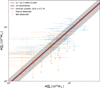 |
Fig. 3 Hydrostatic mass bias determination for Chandra scaling relation, with selection bias accounted for. The clusters detected by Planck are plotted in blue, while the orange points are the mass upper limits for the non-detected clusters. The black line shows the best-fit relation, with red contours corresponding to 1σ uncertainties, and grey contours to the intrinsic scatter. |
Hydrostatic mass biases for both scaling relations.
Scaling relation parameters for both calibration samples.
3.3 Comparison with Planck 2015
Table 2 compares the scaling relation obtained in this work (see Eq. (6)), using Chandra data, to the one obtained by the Planck collaboration, using XMM-Newton data. The scaling relations differ in both normalisation and slope. The lower normalisation obtained in this work is expected given the fact that cluster temperatures measured by Chandra are systematically higher than those measured by XMM-Newton, leading to higher masses (see Schellenberger et al. 2015; Potter et al. 2023). Taking the nonunitary slope of the relation into account, the difference of 20% in normalisation corresponds to a difference in mass of 16%, which corresponds exactly to the expected difference in mass of 16% calculated from the temperature discrepancy between the two telescopes in Schellenberger et al. (2015). It is important to note that the change in normalisation is degenerate with the change in hydrostatic mass bias. Thus, in the fitting process, normalisation and mass bias fully compensate each other given the use of the weak-lensing data as a ‘true’ mass anchor.
The shallower slope can also be explained by the instrumental differences, as the difference in temperature and therefore mass is larger at larger temperatures and masses. This leads to the difference of mass between the least and most massive clusters to be greater in the Chandra sample than in the XMM-Newton sample, and therefore to a shallower slope. We note that the slope obtained in this work is closer to the expected self-similar value of 5/3 (Kravtsov et al. 2006).
Figure 4 shows the mass distribution of the clusters for the full Planck cosmological sample when using the Planck 2015 scaling relation in blue and the relation calibrated in this work in red. In the left panel, the masses are hydrostatic masses, that is, not including a (1 − b) correcting factor, while in the right panel, they are ‘true’ masses, obtained from the full scaling relations, including the bias corrections presented in Table 1. Before bias correction, the change of normalisation of the scaling relation due to differences in instruments and possibly samples is reflected in a shift of the distribution peak, with the Planck scaling relation leading to a peak at lower masses. However, the use of the CCCP/MENeaCS sample as a common ‘true’ mass calibration source and the complete degeneracy between the normalisation and the bias in the scaling relation lead to final mass distributions that peak at the same mass regardless of the calibration sample used. On the other hand, the change of slope in the scaling relation is not degenerate with the bias and does have a slight effect on the mass distribution, leading to a less peaked distribution, with more lower and higher mass clusters.
In terms of uncertainties and scatter, the scaling relations are similar. While this is expected for scatter, one would expect that a scaling relation calibrated on a larger sample would have smaller uncertainties. While this holds for the ![Mathematical equation: $\[Y_{\mathrm{SZ}}-M_{500}^{Y_{\mathrm{X}}}\]$](/articles/aa/full_html/2024/10/aa49513-24/aa49513-24-eq40.png) relations, it is no longer true for the final YSZ − M500 relations, for which the uncertainty on the slope is larger in this work. This can be explained by the difference in the
relations, it is no longer true for the final YSZ − M500 relations, for which the uncertainty on the slope is larger in this work. This can be explained by the difference in the ![Mathematical equation: $\[M_{500}^{Y_{\mathrm{X}}}-M_{500}\]$](/articles/aa/full_html/2024/10/aa49513-24/aa49513-24-eq41.png) relation, which is different for the XMM-Newton and Chandra samples since the X-ray observations were obtained from different instruments. We used Eq. (1) to derive
relation, which is different for the XMM-Newton and Chandra samples since the X-ray observations were obtained from different instruments. We used Eq. (1) to derive ![Mathematical equation: $\[M_{500}^{Y_{\mathrm{X}}}\]$](/articles/aa/full_html/2024/10/aa49513-24/aa49513-24-eq42.png) for the Chandra sample, while the Planck collaboration used the YX − M500 relation from Arnaud et al. (2010) for the XMM-Newton sample. The latter has lower uncertainties, which when propagated, lead to similar uncertainties in the final YSZ − M500 relation, even though the sample used in this work is larger.
for the Chandra sample, while the Planck collaboration used the YX − M500 relation from Arnaud et al. (2010) for the XMM-Newton sample. The latter has lower uncertainties, which when propagated, lead to similar uncertainties in the final YSZ − M500 relation, even though the sample used in this work is larger.
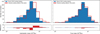 |
Fig. 4 Mass distributions of the clusters of the full Planck cosmological sample, when using the Planck 2015 scaling relation in blue and the relation calibrated in this work in red. The distributions in both panels are obtained from the same sample and identical SZ data. Left: hydrostatic masses i.e. not including a (1 − b) correcting factor, as obtained from Eq. (7). Right: ‘true’ masses, obtained from the full scaling relations including the bias corrections presented in Table 1: |
![Mathematical equation: $\[M_{\text {true }}=\frac{M_{\text {hydrostatic }}}{(1-b)}\]$](/articles/aa/full_html/2024/10/aa49513-24/aa49513-24-eq39.png)
4 Constraining cosmological parameters
To constrain the cosmological parameters Ωm and σ8, we use the procedure from Planck Collaboration XXIV (2016), implemented in the CosmoMC Fortran library (Lewis & Bridle 2002). This section briefly summarises the main steps of the procedure, and the reader is referred to Planck Collaboration XXIV (2016) for more details.
4.1 Modelling and likelihood
4.1.1 Number counts modelling
To constrain the cosmological parameters Ωm and σ8 using cluster number counts, we need a theoretical prediction of cluster abundance as a function of cosmology. We use the mass function from Tinker et al. (2008), which predicts the number of halos per unit mass and volume. On the observation side, the 439 clusters in the Planck cosmological sample are detected using the MMF3 algorithm, based on their SZ signal-to-noise ratio, with a detection threshold of S/N = 6 to ensure a high purity of the sample. Follow-up observations allowed for red-shift determinations. We can thus model the observed cluster number counts as a function of signal-to-noise and redshift, and compare this to the theoretical predictions using the following equation:
![Mathematical equation: $\[\frac{\mathrm{d} N}{\mathrm{d} z \mathrm{d} q}=\int \mathrm{d} \Omega_{\text {mask }} \int \mathrm{d} M_{500} \frac{\mathrm{d} N}{\mathrm{d} z \mathrm{d} M_{500} \mathrm{d} \Omega} P\left[q \mid \bar{q}_{\mathrm{m}}\left(M_{500}, z, l, b\right)\right],\]$](/articles/aa/full_html/2024/10/aa49513-24/aa49513-24-eq43.png) (9)
(9)
where ![Mathematical equation: $\[\frac{\mathrm{d} N}{\mathrm{d}z \mathrm{d} q}\]$](/articles/aa/full_html/2024/10/aa49513-24/aa49513-24-eq44.png) is the observed number counts,
is the observed number counts, ![Mathematical equation: $\[\frac{\mathrm{d} N}{\mathrm{d}z\mathrm{d}M_{500} \mathrm{d} \Omega}\]$](/articles/aa/full_html/2024/10/aa49513-24/aa49513-24-eq45.png) is the product of the mass function times the volume element, q is the signal-to-noise ratio, and
is the product of the mass function times the volume element, q is the signal-to-noise ratio, and ![Mathematical equation: $\[\bar{q}_{\mathrm{m}}\left(M_{500}, z, l, b\right)\]$](/articles/aa/full_html/2024/10/aa49513-24/aa49513-24-eq46.png) is the mean signal-to-noise ratio of a cluster of mass M500 at redshift z. This last term is where the scaling relation, calibrated in the previous section, is used to relate the mass and redshift of a cluster to its expected signal-to-noise ratio:
is the mean signal-to-noise ratio of a cluster of mass M500 at redshift z. This last term is where the scaling relation, calibrated in the previous section, is used to relate the mass and redshift of a cluster to its expected signal-to-noise ratio:
![Mathematical equation: $\[\bar{q}_{\mathrm{m}}=\bar{Y}_{S Z}\left(M_{500}, z\right) / \sigma_{\mathrm{f}}\left[\bar{\theta}_{500}\left(M_{500}, z\right), l, b\right],\]$](/articles/aa/full_html/2024/10/aa49513-24/aa49513-24-eq47.png) (10)
(10)
where ![Mathematical equation: $\[\bar{Y}_{S Z}\left(M_{500}, z\right)\]$](/articles/aa/full_html/2024/10/aa49513-24/aa49513-24-eq48.png) is the mean SZ signal of a cluster of mass m500 at redshift z obtained from the scaling relation, and σf is the noise of the detection filter at the cluster position (l, b) and aperture
is the mean SZ signal of a cluster of mass m500 at redshift z obtained from the scaling relation, and σf is the noise of the detection filter at the cluster position (l, b) and aperture ![Mathematical equation: $\[\bar{\theta}_{500}\]$](/articles/aa/full_html/2024/10/aa49513-24/aa49513-24-eq49.png) . Given a certain cosmology, the aperture is directly linked to the mass and redshift:
. Given a certain cosmology, the aperture is directly linked to the mass and redshift:
![Mathematical equation: $\[\bar{\theta}_{500}=\theta_*\left[\frac{h}{0.7}\right]^{-2 / 3}\left[\frac{(1-b) M_{500}}{3.10^{14} M_{\odot}}\right]^{1 / 3} E^{-2 / 3}(z)\left[\frac{D_A(z)}{500 ~\mathrm{Mpc}}\right]^{-1},\]$](/articles/aa/full_html/2024/10/aa49513-24/aa49513-24-eq50.png) (11)
(11)
with θ* = 6.997 arcmin. The uncertainties and intrinsic scatter of the scaling relation, as well as the noise fluctuations and selection function of the survey are accounted for by the distribution ![Mathematical equation: $\[P\left[q \mid \bar{q}_{\mathrm{m}}\right]\]$](/articles/aa/full_html/2024/10/aa49513-24/aa49513-24-eq51.png) . Following Planck Collaboration XXIV (2016), we use the analytical approximation of the selection function of the Planck survey that assumes pure Gaussian noise, leading to an error function form for the selection function.
. Following Planck Collaboration XXIV (2016), we use the analytical approximation of the selection function of the Planck survey that assumes pure Gaussian noise, leading to an error function form for the selection function.
4.1.2 Likelihood
As in Planck Collaboration XXIV (2016), we use a likelihood constructed in the 2D space of redshift and signal-to-noise ratio, dividing it into 10 redshift bins of width Δz = 0.1 and five signal-to-noise bins of width Δlogq = 0.25. Modelling the observed cluster number counts N(zi, qi) = Nij in each bin as independent Poisson random variables with mean rates ![Mathematical equation: $\[\bar{N}_{i j}\]$](/articles/aa/full_html/2024/10/aa49513-24/aa49513-24-eq52.png) , the log-likelihood is the following:
, the log-likelihood is the following:
![Mathematical equation: $\[\ln \mathcal{L}=\sum_{i, j}\left[N_{i j} \ln \bar{N}_{i j}-\bar{N}_{i j}-\ln \left(N_{i j}!\right)\right].\]$](/articles/aa/full_html/2024/10/aa49513-24/aa49513-24-eq53.png) (12)
(12)
Equation (9) is used to obtain the theoretically predicted mean rates ![Mathematical equation: $\[\bar{N}_{i j}\]$](/articles/aa/full_html/2024/10/aa49513-24/aa49513-24-eq54.png) according to the cosmological parameters and scaling relation:
according to the cosmological parameters and scaling relation:
![Mathematical equation: $\[\bar{N}_{i j}=\frac{\mathrm{d} N}{\mathrm{d} z \mathrm{d} q}\left(z_i, q_j\right) \Delta z \Delta q_j.\]$](/articles/aa/full_html/2024/10/aa49513-24/aa49513-24-eq55.png) (13)
(13)
We map the parameter space using the CosmoMC Monte-Carlo-Markov-Chain sampler using the likelihood in Eq. (12) to constrain the cosmological parameters and obtain the confidence intervals. We consider the standard ΛCDM model, varying the 6 parameters: the baryon density Ωbh2, the cold dark matter density Ωch2, the angular size of the sound horizon at recombination θs, the optical depth to reionisation τ, the amplitude of the primordial power spectrum As, and the spectral index ns. The parameters of the scaling relation are also sampled within the Gaussian priors obtained in Sect. 3.
Similarly to Planck Collaboration XXIV (2016), we need additional information to constrain parameters that cluster number counts are not sensitive to (i.e. all parameters but Ωm and σ8). We add a prior from Big Bang nucleosynthesis (from Steigman 2008) for the value of Ωbh2 = 0.0218 ± 0.0012 and priors from CMB anisotropies (from Planck Collaboration XVI 2014; Planck Collaboration Int. XLVI 2016) for the value of ns = 0.9624 ± 0.014. and τ = 0.055 ± 0.009. While priors from more recent studies could be used, we chose to keep the same priors as in Planck Collaboration XXIV (2016) for full consistency. It should also be noted that while these priors are necessary to generate the halo mass function, their precise value has a very limited impact on the final Ωm and σ8 constraints. We also use the Baryon Acoustic Oscillation (BAO) data from Alam et al. (2017) (BOSS DR12) as an external dataset, using the standard CosmoMC implementation to include it in the likelihood, to help constrain the value of H0 which the number counts alone are unable to.
In the following, we report the constraints in terms of the derived parameters Ωm and σ8, obtained from the underlying parameters Ωbh2, Ωch2, θs, τ, As, and ns.
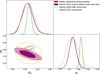 |
Fig. 5 Final cosmological constraints obtained with the scaling relation calibrated in Sect. 3 (in red) and comparison with constraints from SZ number counts obtained in Planck Collaboration XXIV (2016) (in yellow), constraints from CMB primary anisotropies from Planck Collaboration VI (2020) (in green), and constraints obtained using the scaling relation from Planck Collaboration XXIV (2016) with the bias calibrated in Sect. 3.2 (in blue). |
![Mathematical equation: $\[S_{8} \equiv \sigma_{8} \sqrt{\Omega_{m} / 0.3}\]$](/articles/aa/full_html/2024/10/aa49513-24/aa49513-24-eq56.png)
4.2 Cosmological constraints
Figure 5 shows the cosmological constraints obtained in the Ωm − σ8 plane, and compares them to the ones obtained in Planck Collaboration XXIV (2016), the latest constraints from the CMB anisotropies observed by Planck (Planck Collaboration VI 2020), and the constraints obtained when using the scaling relation from Planck Collaboration XXIV (2016) with the bias calibrated in this work. Like all other triangle plots in this work, the GetDist Python package (Lewis 2019) was used to obtain contours from the MCMC chains.
Table 3 shows the constraints on the cosmological parameters for the scaling relation calibrated in Sect. 3 and the Planck scaling relation, updated with the bias calibrated in Sect. 3.2 (XMM-Newton D+nD case) as it is the fairest comparison point to understand the effect of changing only the X-ray calibration sample. The constraints obtained with either calibration sample and the biases computed in this work are in full agreement, both in terms of the central value as well as uncertainties. This is quite remarkable, given the fact that the two samples differ not only in terms of selection function, with the Chandra sample being SZ-selected and the XMM-Newton sample assembled from pre-existing X-ray observations, but also in terms of instruments, with the two samples coming from telescopes known to yield different results in terms of temperature and thus mass estimates, when observing the same clusters (Schellenberger et al. 2015; Potter et al. 2023).
Additionally, the constraints obtained in this work are in agreement with the ones originally obtained in Planck Collaboration XXIV (2016), with similar central values albeit better constraining power in the S8 direction, due to an improved calibration of the mass bias, thanks to the larger weak-lensing dataset from Herbonnet et al. (2020) used in this re-analysis.
5 Discussion
5.1 Possible sources of systematic uncertainties
In this Section, we provide an overview of several sources of systematic error that could cause a shift in the cosmological constraints, and try to quantify the effect whenever possible.
Mass function. Like every study of galaxy cluster number counts, a choice of reference halo mass function has to be made when comparing the observed cluster abundance with the theoretical predictions. For our analysis, we chose to use the Tinker et al. (2008) mass function for consistency with the baseline Planck Collaboration XXIV (2016) analysis. In the Planck analysis, changing the halo mass function was found to shift the final value of Ωm up by ~10% and the final value of σ8 down by ~10% as well. Since we use the same cluster catalogue and simply change the mass calibration, we expect a very similar shift in the final constraints if we were to change the mass function to that of Watson et al. (2013) as well. More recently, Abbott et al. (2020) and Bocquet et al. (2024) have tried to quantify the uncertainties around the Tinker et al. (2008) mass function using other simulations. Bocquet et al. (2024) compared marginalising over those uncertainties with not accounting for them and found no significant shifts in the final constraints, thus concluding that the uncertainties on the halo mass function could be neglected.
Weak-lensing mass bias. Calibrating the mass bias from weak-lensing data requires the assumption that the weak-lensing mass estimates are unbiased. However, it has been shown that weak-lensing mass estimates can be subject to systematic biases (see e.g. Grandis et al. 2024; Bocquet et al. 2023). In this work, we do not explicitly correct for these systematic biases as we use masses taken from Herbonnet et al. (2020) which are already corrected by comparing with simulations (see Appendix C of Herbonnet et al. 2020, for an extensive description of the correction procedure).
Mass calibration at fixed cosmology. A caveat of the approach is that the scaling relation is obtained for a fixed cosmology, while the value of the parameters varies during the MCMC fitting. The reason for this is two-fold: first, since this work aims at studying the impact of the mass calibration, we thus chose to keep all other elements of the procedure identical to Planck Collaboration XXIV (2016). Also, a fully consistent approach would require the re-extraction of X-ray data at every step, as a fixed cosmology is also assumed during the data reduction process. Overall, the effect of varying the cosmology within the 2σ contours we obtain yields a maximum difference of 2% in X-ray mass for the highest redshift clusters in the calibration sample, and less than 1% for most of the sample. This is smaller than the uncertainties on the mass calibration, and we thus expect the effect to be negligible with respect to the other sources of uncertainty.
Miscentering of MMF detections. When calibrating the scaling relation, we have access to a very precise position and size prior from the X-ray data, as the Chandra telescope has a very good angular resolution of 0.5 arc-seconds (6 arc-seconds for XMM-Newton). We make use of that prior to perform pointed detection with the MMF algorithm in the Planck data, as blind detections are not only more computationally expensive, but also less precise due to Planck’s larger point spread function of ~7 arc-minutes. However, the PSZ2 catalogue that we use to constrain the cosmology is obtained from blind detections of clusters, which could cause biases in the retrieved SZ signal. This issue was investigated in Planck Collaboration XX (2014), where a good agreement was found between the signal-to-noise ratio for blind and pointed detections (see Fig. 2 of that paper). Given the fact that we are binning the clusters into quite large S/N bins, we expect the small scatter between the two S/N estimates to be negligible.
Correct retrieval of the scaling relation. With the increased precision of the mass calibration via scaling relation presented in this work, we need to ensure that the accuracy of the method is sufficient to not induce a systematic bias in the final constraints. To verify this, we generated 100 synthetic cluster samples resembling the Chandra sample with realistic observables, following a known underlying scaling relation (see Appendix C for details on the sample generation). We then ran these samples through the scaling relation calibration pipeline, and compared the retrieved relations with the true underlying relation.
The results of the comparison are presented in Fig. 6, which shows that the calibration procedure retrieves the underlying scaling relation with very good accuracy and correctly estimated uncertainties. In particular, the parameter combination ![Mathematical equation: $\[(1-b)^{\alpha} 10^{Y^{*}}\]$](/articles/aa/full_html/2024/10/aa49513-24/aa49513-24-eq57.png) , which sets the mass scale and is by far the most important parameter in terms of final cosmological constraints is perfectly retrieved. In comparison, the very slight bias of around 0.5σ (the mean retrieved value being 1.72 for a true value of 1.70) that can arguably be observed on the slope would result in no shift at all in final cosmological constraints. Indeed, identical constraints are obtained with the Chandra and XMM-Newton calibration sample, even though they result in a slope difference four times larger than the bias found here. Similarly, the difference between the mean retrieved intrinsic scatter and the true value is much smaller than the difference between those obtained with the two calibration samples, and would thus not affect the final constraints at all. Using the same population generation procedure, we also show that the possible presence of correlated intrinsic scatter between YSZ and YX would not lead to a significant bias in the final constraints (see Appendix C for more details).
, which sets the mass scale and is by far the most important parameter in terms of final cosmological constraints is perfectly retrieved. In comparison, the very slight bias of around 0.5σ (the mean retrieved value being 1.72 for a true value of 1.70) that can arguably be observed on the slope would result in no shift at all in final cosmological constraints. Indeed, identical constraints are obtained with the Chandra and XMM-Newton calibration sample, even though they result in a slope difference four times larger than the bias found here. Similarly, the difference between the mean retrieved intrinsic scatter and the true value is much smaller than the difference between those obtained with the two calibration samples, and would thus not affect the final constraints at all. Using the same population generation procedure, we also show that the possible presence of correlated intrinsic scatter between YSZ and YX would not lead to a significant bias in the final constraints (see Appendix C for more details).
Double systems. Given the ~7 arc-minutes Planck beam, two clusters that are roughly aligned along the line of sight can lead to a single detection in the Planck maps. During the mass calibration process, we can avoid this problem thanks to the much higher resolution X-ray images that allow us to remove such double systems from the calibration sample. Nevertheless, these systems cannot be identified when compiling the PSZ2 catalogue used to constrain the cosmology. Given the abundance of double systems in the calibration, we can expect around 16 out of the 439 clusters in the PSZ2 sample to be double systems. It is hard to predict the effect of the presence of double systems on the final results as it is not possible to know a priori the effect on the S/N of detection. We can however expect that the magnitude of the bias in the final constraints is small given the small number of double systems that are likely present in the PSZ2 sample.
Implementation of the likelihood. The implementation of the likelihood is the same as in Planck Collaboration XXIV (2016), which was validated by comparing three independent implementations which were found to yield differences in cosmological constraints of less than 1/10 σ. Given that the maximal improvement of constraining power compared to Planck Collaboration XXIV (2016) is a factor of two on the value of S8, the uncertainty coming from the implementation of the likelihood is still negligible in this work.
In conclusion, the halo mass function is the main source of systematic uncertainty. The magnitude of this systematic uncertainty is such that all other effects are negligible in comparison. The calibration of the halo mass function is the subject of ongoing research and debate in the community, and as such is outside the scope of this study. Nevertheless, the recent results of Bocquet et al. (2024) seem to indicate that the impact of the uncertainty on the mass function on SZ cluster number count cosmology studies might not be as important as that estimated in Planck Collaboration XXIV (2016), with recent simulation results being in reasonably good agreement with each other.
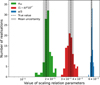 |
Fig. 6 Retrieved YSZ − M500 scaling relation on 100 synthetic calibration samples compared with the true underlying relation used for sample generation. The retrieved slope (divided by three for better readability) is shown in blue, the retrieved intrinsic scatter in green, and the relevant combination of the degenerated parameters (1 − b) and Y* in red. The true value of each parameter is shown by the black dashed lines and the mean uncertainty returned by the calibration procedure is shown by the grey contours. |
5.2 Exploring the redshift dependence
When calibrating the scaling relation in Sect. 3, we fixed the redshift dependence of the relation to the self-similar value of −2/3 in order to follow the calibration process of Planck Collaboration XX (2014). However, if we split the sample into two sub-samples with clusters below or above the median redshift of the full sample of z = 0.15 and calibrate the scaling relation on each sub-sample independently, the resulting best fits are in disagreement. Figure 7 shows the scaling relations calibrated on the two sub-samples, and compares them with the best fit obtained on the full sample. For both sub-samples, the best-fit relation has a shallower slope than the one obtained on the full sample by more than 1σ, and the low-z (respectively high-z) best-fit relation has a lower (resp. higher) normalisation than the scaling relation obtained with the full sample. This suggests that the assumed self-similar redshift dependence cannot properly fit the data over the entire redshift range of the sample.
To explore this further, we fit the scaling relation with a free redshift dependence, using the following relation:
![Mathematical equation: $\[E^\beta(z) \frac{D_A^2 Y_{\mathrm{SZ}}}{Y_{\mathrm{piv}}}=10^{Y^*}\left(\frac{M_{500}^{Y_{\mathrm{X}}}}{M_{\mathrm{piv}}}\right)^\alpha.\]$](/articles/aa/full_html/2024/10/aa49513-24/aa49513-24-eq59.png) (14)
(14)
We add an additional free parameter to the equation, letting the power of E(z) vary from the self-similar value of −2/3, and modify the likelihood presented in Sect. 3.1 to account for this additional degree of freedom. We use a broad, flat prior on β. Fig. 8 shows the best-fit relation obtained with this model. The best-fit value for the redshift dependence is β = −2.22 ± 0.45, which is in tension with the self-similar value of −2/3 at more than 3σ. Introducing this degree of freedom in the scaling relation also reduces the intrinsic scatter (σint = 17.8% instead of 19.6%), and lowers the mass dependence to α = 1.59 ± 0.05, below the 5/3 value predicted by the self-similar model by 1σ.
To verify if this is simply a trend in this particular sample, we repeat the same analysis on the XMM-Newton sample. We obtain a best-fit value of β = −1.96 ± 0.47, in agreement with the one obtained on the Chandra sample and in roughly 3σ tension with the self-similar value. We also observe a similar decrease in intrinsic scatter (14.8% from 15.8%), and the mass dependence that initially was steeper than the self-similar value is in perfect agreement with it at 1.66 ± 0.078.
Andreon (2014) performed a similar calibration of the Planck Ysz − M500 relation letting the redshift dependence vary, and found β = −2.5 ± 0.4, which is in agreement with the results found here. Another result we can compare with is the redshift-dependent bias presented in Sect. 6.4 of Sereno & Ettori (2017). The authors computed the best-fit bias between the weak-lensing masses they compiled and the Planck masses (obtained with the scaling relation from Planck Collaboration XX (2014), i.e. with a self-similar redshift dependence) for a set of clusters where both mass estimates were available. They allowed for both redshift- and mass-dependence, and found
![Mathematical equation: $\[M_{\mathrm{SZ}}=(1.05 \pm 0.11) M_{\mathrm{WLc}}^{0.94 \pm 0.08}\left(\frac{E(z)}{E\left(z_{\text {ref }}\right)}\right)^{-2.40 \pm 0.63}.\]$](/articles/aa/full_html/2024/10/aa49513-24/aa49513-24-eq60.png) (15)
(15)
While the deviation of the mass dependence from unity is negligible, their result points to a strong redshift dependence, with SZ-masses of high-redshift clusters being biased lower with respect to WL-masses than those of low-redshift clusters. If we were to recompute this bias using SZ-masses obtained with the modified scaling relation presented in Table 4, we would expect the redshift dependence of the bias to change, as it would be affected by the non-self-similar redshift evolution of the scaling relation used to compute the SZ-masses. While performing the fit is outside the scope of this study, we can expect a change of redshift dependence of the order of ![Mathematical equation: $\[\frac{-2 / 3-\beta}{\alpha} \sim 1\]$](/articles/aa/full_html/2024/10/aa49513-24/aa49513-24-eq61.png) , raising the best-fit value of the redshift dependence from −2.4 to roughly −1.4. While an even larger departure from the self-similar redshift evolution of the YSZ − M500 relation would be needed to fully explain the redshift dependence of the bias, the deviation from self-similar redshift evolution computed in this study can explain a significant part of the effect observed in Sereno & Ettori (2017). Other sources of biases, in the weak-lensing mass computation for example, are still left to be explored and could explain the rest of the redshift dependence of the SZ-mass to WL-mass bias.
, raising the best-fit value of the redshift dependence from −2.4 to roughly −1.4. While an even larger departure from the self-similar redshift evolution of the YSZ − M500 relation would be needed to fully explain the redshift dependence of the bias, the deviation from self-similar redshift evolution computed in this study can explain a significant part of the effect observed in Sereno & Ettori (2017). Other sources of biases, in the weak-lensing mass computation for example, are still left to be explored and could explain the rest of the redshift dependence of the SZ-mass to WL-mass bias.
Wicker et al. (2023) investigated the evolution of the hydrostatic mass bias with mass and redshift by studying the evolution of the gas fraction in galaxy clusters. They found
![Mathematical equation: $\[(1-b)=(0.83 \pm 0.04)\left(\frac{M}{\langle M\rangle}\right)^{-0.06 \pm 0.04}\left(\frac{1+z}{\langle 1+z\rangle}\right)^{-0.64 \pm 0.18}.\]$](/articles/aa/full_html/2024/10/aa49513-24/aa49513-24-eq62.png) (16)
(16)
Similarly to Sereno & Ettori (2017), the mass dependence is negligible, but they found a significant negative redshift dependence. Following the same reasoning as above, the deviation from self-similar redshift evolution found in this work would correspond to redshift evolution of (1 − b) of around −1, which, while not fully compatible, is coherent with the negative value found by Wicker et al. (2023).
Given the fact that both calibration samples show a similar and significant deviation from the self-similar redshift dependence, even though their selection function is very different (SZ-selected for Chandra, pre-existing X-ray observation for XMM-Newton), and that other results in the literature point to a similar deviation, we conclude that this is likely not a selection effect, but rather a systematic effect, stemming either from actual physical processes not properly described by the self-similar model or from untreated systematics in the instrument or data extraction.
Lovisari et al. (2017) provides morphological information for 92 clusters in the Chandra sample, which we can make use of to further investigate this redshift dependence question. When fitting the redshift dependence of the scaling relation on the 32 clusters with a relaxed morphology, the best fit value is β = −2.5 ± 1.3, which is steeper than the value obtained on the full sample (while still being in general agreement). When fitting the redshift dependence of the scaling relation on the 60 clusters with a mixed or disturbed morphology, the best-fit value is β = −1.1 ± 0.8, which is shallower than the value obtained on the full sample, and closer to the self-similar value of −2/3. Although the statistical significance is low, this suggests that the deviation from the self-similar model might be related to the dynamical state of the clusters, and that relaxed, high redshift clusters exhibit a lack of YSZ signal compared to their X-ray derived mass. A possible explanation for this behaviour is the fact that Planck-detected clusters at redshifts above z~0.15 are smaller than the beam of the instrument. This leads to a large smoothing of the cluster signal, which is accounted for in the MMF detection by using templates of both the cluster profile and the beam. Since neither of these templates is guaranteed to be fully accurate, this could lead to an incorrect extraction of the YSZ signal, especially for relaxed clusters, which likely have a more peaked profile, prone to larger smoothing.
We use these newly obtained scaling relations to constrain cosmological parameters, and compare the results with the ones obtained with the self-similar scaling relations. We follow the procedure described in Sects. 3 and 4, with the only difference being the use of the new scaling relations. The first step is to combine these new ![Mathematical equation: $\[Y_{\mathrm{SZ}}-M_{500}^{Y_{\mathrm{X}}}\]$](/articles/aa/full_html/2024/10/aa49513-24/aa49513-24-eq63.png) relations with the respective
relations with the respective ![Mathematical equation: $\[M_{500}^{Y_{\mathrm{X}}}-M_{500}\]$](/articles/aa/full_html/2024/10/aa49513-24/aa49513-24-eq64.png) relations to obtain the YSZ − M500 relations. From these scaling relations, we can extract the bias, following the same procedure as in Sect. 3.2. Table 4 shows the YSZ − M500 relations from which cosmological constraints will be derived. With the scaling relations fully calibrated, we can constrain the cosmological parameters, following the same procedure as in Sect. 4. Figure 9 shows the cosmological constraints obtained with the new scaling relations, and compares them to the ones obtained with the self-similar scaling relation calibrated on the Chandra sample. Table 5 presents the constraints on the cosmological parameters. There is a significant loss in constraining power, especially along the Ωm − σ8 degeneracy, given the introduction of a new degree of freedom in the scaling relation, but we can still observe a preference for higher
relations to obtain the YSZ − M500 relations. From these scaling relations, we can extract the bias, following the same procedure as in Sect. 3.2. Table 4 shows the YSZ − M500 relations from which cosmological constraints will be derived. With the scaling relations fully calibrated, we can constrain the cosmological parameters, following the same procedure as in Sect. 4. Figure 9 shows the cosmological constraints obtained with the new scaling relations, and compares them to the ones obtained with the self-similar scaling relation calibrated on the Chandra sample. Table 5 presents the constraints on the cosmological parameters. There is a significant loss in constraining power, especially along the Ωm − σ8 degeneracy, given the introduction of a new degree of freedom in the scaling relation, but we can still observe a preference for higher ![Mathematical equation: $\[S_{8} \equiv \sigma_{8} \sqrt{\Omega_{m} / 0.3}\]$](/articles/aa/full_html/2024/10/aa49513-24/aa49513-24-eq65.png) values (S8 = 0.811 ± 0.020 with the Chandra calibration sample), closer to the results of the CMB primary anisotropies of Planck Collaboration VI (2020). This is due to the fact that the steeper redshift dependence, combined with the low median redshift of the X-ray and WL calibration samples (z~0.2), lead to more massive clusters at high redshifts than the self-similar model and thus to a higher matter density and/or more clustered matter distribution.
values (S8 = 0.811 ± 0.020 with the Chandra calibration sample), closer to the results of the CMB primary anisotropies of Planck Collaboration VI (2020). This is due to the fact that the steeper redshift dependence, combined with the low median redshift of the X-ray and WL calibration samples (z~0.2), lead to more massive clusters at high redshifts than the self-similar model and thus to a higher matter density and/or more clustered matter distribution.
While cosmological constraints where the redshift dependence is left free to vary are presented in Fig. 6 of Planck Collaboration XXIV (2016), a direct comparison is not relevant, since the fitting procedures are completely different. In this work, we fit the redshift dependence as part of the mass calibration, simultaneously fitting Y*, α, and β, then computing the hydrostatic mass bias (1 − b) with the previously obtained relation, and finally fitting the observed number counts to constrain the cosmology. In Planck Collaboration XXIV (2016), the constraints are obtained by using the same scaling relation as in the self-similar redshift evolution case, but simply replacing the prior that fixed the redshift dependence to an uninformative flat prior when fitting the observed number counts. Since the value of the other parameters of the scaling relation is not coherently fitted with the redshift evolution, it is expected that the impact on the final constraints is not as important as in this work. In particular, no change in the final S8 value is observed in Planck Collaboration XXIV (2016).
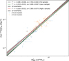 |
Fig. 7 Calibration of the |
![Mathematical equation: $\[Y_{\mathrm{SZ}}-M_{500}^{Y_{\mathrm{X}}}\]$](/articles/aa/full_html/2024/10/aa49513-24/aa49513-24-eq58.png)
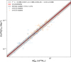 |
Fig. 8 Calibration of the YSZ − scaling relation, letting the redshift dependence vary as a free parameter. The high and low redshift subsamples are shown in different colours to help visualise the effect of the free redshift dependence, but the fit is performed on the whole sample at once. The black line shows the best-fit relation, with red contours corresponding to 1σ uncertainties, and grey contours to the intrinsic scatter. |
YSZ − M500 scaling relations with free redshift dependence for both calibration samples.
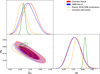 |
Fig. 9 Cosmological constraints obtained with the redshift dependence fitted from the data, with both Chandra (in red) and XMM-Newton (in blue) calibration samples, and comparison with the results obtained with the fixed, self-similar redshift dependence using the Chandra calibration sample (in yellow) and Planck Collaboration VI (2020) constraints from CMB primary anisotropies (in green). |
![Mathematical equation: $\[S_{8} \equiv \sigma_{8} \sqrt{\Omega_{m} / 0.3}\]$](/articles/aa/full_html/2024/10/aa49513-24/aa49513-24-eq66.png)
χ2/NDoF value of the fits performed during the mass calibration.
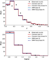 |
Fig. 10 Redshift (top panel) and signal-to-noise (bottom panel) distribution of best-fit models from the four analysis cases presented in this work. The observed counts in the PSZ2 catalogue (q > 6) are plotted as the black points. |
5.3 Goodness of fit
In this analysis, there are several fitting procedures during both the mass calibration and the cosmological constraints steps for which we should investigate the goodness of fit. To evaluate the goodness of fit of the scaling relations, we present in Table 6 the χ2 value compared to the number of degrees of freedom NDoF of the various fits performed in this work.
We find that all fits showχ2 values close to NDoF, indicating a good fit of the data by the model. We also find that for both calibration samples, fitting the redshift evolution β from the data improves the goodness of fit of the ![Mathematical equation: $\[Y_{\mathrm{SZ}}-M_{500}^{Y_{\mathrm{X}}}\]$](/articles/aa/full_html/2024/10/aa49513-24/aa49513-24-eq68.png) scaling relation as well as the hydrostatic mass bias (1 − b).
scaling relation as well as the hydrostatic mass bias (1 − b).
Figure 10 presents the redshift and signal-to-noise distribution of the best-fit models for all four analysis cases considered in this work, and compares them to the observed number counts of the PSZ2 catalogue. Since the number counts are fitted with a Poisson likelihood and some bins contain very few clusters, the most relevant statistic to evaluate the goodness of fit is the C statistic (see e.g. Bonamente 2020, for details on the C statistic). Table 7 presents the C statistic value found for the four analysis cases for which cosmological parameters were fitted in this work.
We find that the fit of the number counts is acceptable but not optimal, and that the various analysis cases do not lead to a significantly different goodness of fit. This is due to the fact that the distribution of the PSZ2 clusters in redshift does not accurately follow that of the best-fit mass function prediction (see also Fig. 6 of Planck Collaboration XXIV 2016, where the same problem was observed). Since this work only changes the mass calibration and has a limited impact on the best-fit cosmology, this issue is not solved.
C statistic value of the number count fits.
5.4 Comparison with other cosmological analyses
Fig. 11 shows the ![Mathematical equation: $\[S_{8} \equiv \sigma_{8} \sqrt{\Omega_{m} / 0.3}\]$](/articles/aa/full_html/2024/10/aa49513-24/aa49513-24-eq69.png) constraints obtained in this work compared to the ones obtained in a few other recent analyses using both cluster number counts as well as other different cosmological probes. We selected analyses that presented constraints on S8 using the definition chosen in this work for consistency. It is important to note that, while necessary to compare different results, this definition is not necessarily the optimal one for each probe, in the sense that errors might be smaller for another power of Ωm.
constraints obtained in this work compared to the ones obtained in a few other recent analyses using both cluster number counts as well as other different cosmological probes. We selected analyses that presented constraints on S8 using the definition chosen in this work for consistency. It is important to note that, while necessary to compare different results, this definition is not necessarily the optimal one for each probe, in the sense that errors might be smaller for another power of Ωm.
We compiled results from Planck Collaboration XXIV (2016) (noted Planck15 SZ), Bocquet et al. (2019) & Bocquet et al. (2024) (SPT SZ cluster number counts), Ghirardini et al. (2024) (eROSITA cluster number counts), Garrel et al. (2022) (analysis of an XMM-Newton-selected cluster sample), Costanzi et al. (2021) (DES+SPT cluster abundance), Amon et al. (2022) (DES Y3 cosmic shear), Heymans et al. (2021) (KiDS1000 WL + galaxy clustering), Li et al. (2023) (HSC cosmic shear), Planck Collaboration VI (2020) (noted Planck18 CMB), Aiola et al. (2020) (ACT DR4 CMB), Balkenhol et al. (2023) (SPT-3G CMB), and Madhavacheril et al. (2024) (ACT DR6 CMB gravitational lensing). For clarity of the plot, we had to pick one HSC result amongst four different analyses, but Dalal et al. (2023), Miyatake et al. (2023), and Sugiyama et al. (2023) all find very similar results to the one chosen for the comparison.
With this re-analysis, S8 constraints from SZ number counts are competitive with the tightest constraints obtained from CMB primary anisotropies in Planck Collaboration VI (2020) or from the latest cosmic shear surveys in Amon et al. (2022) and Heymans et al. (2021), even when the redshift dependence is left free to vary. With this improved constraining power, we can use clusters to investigate the S8 tension, as they now provide constraints tight enough to reject either the S8~0.77 value preferred by most late-time probes or the S8~0.83 value preferred by most CMB experiments with higher significance than previous results. Regardless of the calibration sample, we find that the constraints obtained with the self-similar redshift evolution agree with the values derived from the latest weak-lensing analyses (Amon et al. 2022; Heymans et al. 2021), and are in tension with the Planck CMB constraints at around 2σ. If we fit the redshift dependence of the scaling relation from the data, the derived S8 constraints shift to higher values by about 1σ and are right in-between values obtained by the latest WL analyses and those obtained by the latest CMB experiments, resulting in no significant tension with either result.
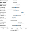 |
Fig. 11 Comparison of the S8 constraints obtained in this work (in bold) with other recent analyses. |
6 Conclusion
Using a new full follow-up observation of the Planck ESZ sample with the Chandra X-ray telescope, we have calibrated a new YSZ − M500 scaling relation using a sample of 146 clusters. Using the weak-lensing sample from Herbonnet et al. (2020) as an external mass calibration, we have also estimated the hydrostatic mass bias for both the newly calibrated scaling as well as the scaling relation calibrated in Planck Collaboration XX (2014). When accounting for clusters not detected in the Planck maps, we found a mass bias of (1 − b) = 0.89 ± 0.04 for the new scaling relation, and (1 − b) = 0.76 ± 0.04 for the Planck scaling relation.
Using these scaling relations, we obtained cosmological constraints on Ωm and σ8 from the Planck cosmological sample. We found that the constraints we obtained with both calibration samples are identical, with σ8 = 0.77 ± 0.02, Ωm = 0.31 ± 0.02, and ![Mathematical equation: $\[S_{8} \equiv \sigma_{8} \sqrt{\Omega_{m} / 0.3}=0.78 \pm 0.02\]$](/articles/aa/full_html/2024/10/aa49513-24/aa49513-24-eq70.png) . These constraints are in agreement with the ones obtained in Planck Collaboration XXIV (2016), albeit with a much tighter constraint on S8.
. These constraints are in agreement with the ones obtained in Planck Collaboration XXIV (2016), albeit with a much tighter constraint on S8.
We also investigated deviations from self-similar redshift evolution of the YSZ − M500 relations and found that letting the redshift dependence as a free parameter when fitting the relation with either calibration sample led to similar values of β~−2 in significant tension with the self-similar value β = −2/3. We constrained the cosmology with the scaling relations calibrated with a free redshift dependence and found essentially identical results with both X-ray calibration samples, with σ8 = 0.76 ± 0.03, Ωm = 0.34 ± 0.03, and ![Mathematical equation: $\[S_{8} \equiv \sigma_{8} \sqrt{\Omega_{m} / 0.3}=0.81 \pm 0.02\]$](/articles/aa/full_html/2024/10/aa49513-24/aa49513-24-eq71.png) .
.
Compared to results from other probes, they are competitive with analyses of CMB primary anisotropies and cosmic shear in terms of S8 constraining power. Like most analyses of galaxy clusters and other late-time probes, with the exceptions of the XXL survey (Garrel et al. 2022) and the recent eROSITA results presented in Ghirardini et al. (2024), the cosmological constraints derived in this work show a lower central value of S8 than what is usually found by CMB primary anisotropies analyses. It is important to note that while the central value is lower, none of the four sets of constraints presented here exhibit a strong tension with the latest Planck CMB constraints, with differences ranging from around 2σ in the self-similar redshift evolution case and less than 1σ when fitting the redshift dependence from the data.
This work shows that SZ cluster surveys are a powerful tool to constrain cosmology, and that the mass calibration of the clusters is paramount to the constraining power. In the coming years, the next generation of CMB experiments will detect an increasing number of clusters, and a robust mass calibration will be necessary to fully exploit these surveys. Such a mass calibration could be provided by the coming weak-lensing and X-ray surveys, that will detect tens of thousands of clusters across a large redshift range.
Acknowledgements
G.A. acknowledges financial support from the AMX program. This work was supported by the French Space Agency (CNES). This work was supported by the Programme National Cosmology et Galaxies (PNCG) of CNRS/INSU with INP and IN2P3, co-funded by CEA and CNES. This research has made use of the computation facility of the Integrated Data and Operation Center (IDOC, https://idoc.ias.u-psud.fr) at the Institut d’Astrophysique Spatiale (IAS), as well as the SZ-Cluster Database (https://szdb.osups.universite-paris-saclay.fr). W.F. acknowledges support from the Smithsonian Institution, the Chandra High-Resolution Camera Project through NASA contract NAS8-0306, NASA Grant 80NSSC19K0116 and Chandra Grant GO1-22132X. F.A.-S. acknowledges support from Chandra Grant GO0-21119X. R.J.v.W. acknowledges support from the ERC Starting Grant ClusterWeb 804208.
Appendix A Calculation of cluster masses from Planck catalogue data
The Planck MMF3 catalogue provides the 2D posterior probability distribution in θs and ![Mathematical equation: $\[Y_{5 R_{500}}\]$](/articles/aa/full_html/2024/10/aa49513-24/aa49513-24-eq72.png) for each cluster (see Planck Collaboration XXVII 2016, for the full details). Computing masses from these distributions, given a YSZ − M500 scaling relation, is not straightforward, since the aperture in which the SZ signal is measured depends on R500, and thus on the cluster mass. To ensure that apertures and masses are coherent, we make use of a second scaling relation between θ500 and M500. Unlike the YSZ − M500 relation, this relation is not calibrated on data but is just a direct consequence of the underlying cosmological model. For the flat ΛCMD cosmology used in this work, the relation is the following:
for each cluster (see Planck Collaboration XXVII 2016, for the full details). Computing masses from these distributions, given a YSZ − M500 scaling relation, is not straightforward, since the aperture in which the SZ signal is measured depends on R500, and thus on the cluster mass. To ensure that apertures and masses are coherent, we make use of a second scaling relation between θ500 and M500. Unlike the YSZ − M500 relation, this relation is not calibrated on data but is just a direct consequence of the underlying cosmological model. For the flat ΛCMD cosmology used in this work, the relation is the following:
![Mathematical equation: $\[\theta_{500}=\theta_*\left[\frac{h}{0.7}\right]^{-2 / 3}\left[\frac{M_{500}}{3.10^{14} M_{\odot}}\right]^{1 / 3} E^{-2 / 3}(z)\left[\frac{D_A(z)}{500 ~\mathrm{Mpc}}\right]^{-1},\]$](/articles/aa/full_html/2024/10/aa49513-24/aa49513-24-eq73.png) (A.1)
(A.1)
where θ*=6.997 arcmin.
To obtain masses from the posterior distributions, we use a Monte-Carlo-Markov-Chain (MCMC) approach, using emcee as the sampler. At each step of the chain, we draw values of mass and scaling relation parameters. We then compute the corresponding θ500 and YSZ, and use them to obtain the likelihood from the observed ![Mathematical equation: $\[\theta_{s}-Y_{5 R_{500}}\]$](/articles/aa/full_html/2024/10/aa49513-24/aa49513-24-eq74.png) probability distribution. We then combine this likelihood with the Gaussian priors on the scaling relation parameters to obtain the final likelihood used to run the chain. The mass is then obtained as the mean of the posterior distribution, with the standard deviation as the uncertainty. Fig. A.1 plots 100 samples taken at random from the MCMC mass estimation procedure of the PSZ2 G033.97-76.61 cluster over the 2D probability map found in the PSZ2 catalogue.
probability distribution. We then combine this likelihood with the Gaussian priors on the scaling relation parameters to obtain the final likelihood used to run the chain. The mass is then obtained as the mean of the posterior distribution, with the standard deviation as the uncertainty. Fig. A.1 plots 100 samples taken at random from the MCMC mass estimation procedure of the PSZ2 G033.97-76.61 cluster over the 2D probability map found in the PSZ2 catalogue.
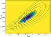 |
Fig. A.1 100 samples taken at random from the MCMC mass estimation procedure of the PSZ2 G033.97-76.61 cluster plotted over the 2D probability map from the MMF3 detection found in the PSZ2 catalogue. |
Appendix B Importance of proper non-detection treatment in bias estimations
Fig. B.1 shows the difference in the final cosmological constraints with the same scaling relation, but using either the bias calibrated using only the cluster detected by Planck (D bias) or also accounting for non-detections (D+nD bias). The shift in the constraints is small, with a preference for slightly higher values of σ8 and marginally better constraining power when accounting for non-detections: ![Mathematical equation: $\[\sigma_{8}^{\mathrm{D}+\mathrm{nD}}=0.765 \pm 0.019, \sigma_{8}^{\mathrm{D}}=0.760 \pm 0.020\]$](/articles/aa/full_html/2024/10/aa49513-24/aa49513-24-eq75.png) . The value and uncertainty of Ωm are not affected.
. The value and uncertainty of Ωm are not affected.
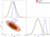 |
Fig. B.1 Final cosmological constraints obtained with the bias calculated not including the non-detections (in green) or taking them into account (in red). |
Appendix C Synthetic sample generation
In order to verify that our mass calibration pipeline retrieves the correct underlying scaling relation, we generate realistic mock calibration samples with a known underlying scaling relation and run them through the scaling relation calibration pipeline. We first create a 2D number counts array by Poisson sampling the Tinker et al. (2008) halo mass function, calculated using the hmf Python package (Murray et al. 2013), in 350 redshift bins between z = 0 and z = 0.5 and 500 M500 bins between 1014 and 1016 M⊙. We attribute to each cluster a true X-ray mass,
![Mathematical equation: $\[M_{500}^{\mathrm{X}, \text { true }}=(1-b) M_{500} e^{x_1},\]$](/articles/aa/full_html/2024/10/aa49513-24/aa49513-24-eq76.png) (C.1)
(C.1)
a true weak-lensing mass, and
![Mathematical equation: $\[M_{500}^{\mathrm{WL}, \text { true }}=M_{500} e^{x_2},\]$](/articles/aa/full_html/2024/10/aa49513-24/aa49513-24-eq77.png) (C.2)
(C.2)
a true SZ-signal,
![Mathematical equation: $\[Y_{\mathrm{SZ}, \text { true }}=Y_{\mathrm{piv}} \frac{E^{2 / 3}(z) 10^{Y^*}}{D_A^2}\left(\frac{M_{500}^{Y_{\mathrm{X}}}}{M_{\mathrm{piv}}}\right)^\alpha e^{x_3},\]$](/articles/aa/full_html/2024/10/aa49513-24/aa49513-24-eq78.png) (C.3)
(C.3)
where the xi variables are used to generate random log-normal intrinsic scatter, with the following:
![Mathematical equation: $\[P\left(x_i\right)=\mathcal{N}\left(\left[\begin{array}{l}0 \\0 \\0\end{array}\right] \Sigma\right) \text {, where } \Sigma=\left[\begin{array}{ccc}\sigma_{\mathrm{X}}^2 & 0 & \rho \sigma_{\mathrm{X}} \sigma_{\mathrm{SZ}} \\0 & \sigma_{\mathrm{WL}}^2 & 0 \\\rho \sigma_{\mathrm{X}} \sigma_{\mathrm{SZ}} & 0 & \sigma_{\mathrm{SZ}}^2\end{array}\right] \text {. }\]$](/articles/aa/full_html/2024/10/aa49513-24/aa49513-24-eq79.png) (C.4)
(C.4)
We note that we allow for correlated intrinsic scatter between X-ray mass and SZ-signal, since the X-ray masses in the real data are derived from YX which might show correlation with YSZ. In the main body, we presented results for no correlation, but we conducted the study for ρ = [0, 0.25, 0.5, 0.75, 1] to quantify the effect of this potential correlation.
We use a simple neural network (two-layer perceptron with 1000 units each) trained on the actual data to generate realistic uncertainties on the X-ray masses given the X-ray mass and redshift. We multiply the output of the network by a random log-normal component to add randomness to the uncertainties to best match the actual data. We repeat the same procedure to generate uncertainties on the WL masses. We then obtain measured X-ray and WL masses ![Mathematical equation: $\[M_{500}^{\mathrm{X}, \text { mes }}\]$](/articles/aa/full_html/2024/10/aa49513-24/aa49513-24-eq80.png) and
and ![Mathematical equation: $\[M_{500}^{\mathrm{WL} \text {, mes }}\]$](/articles/aa/full_html/2024/10/aa49513-24/aa49513-24-eq81.png) by adding a random Gaussian component, with mean 0 and standard deviation the uncertainty previously generated, to
by adding a random Gaussian component, with mean 0 and standard deviation the uncertainty previously generated, to ![Mathematical equation: $\[M_{500}^{\mathrm{X}, \text { true }}\]$](/articles/aa/full_html/2024/10/aa49513-24/aa49513-24-eq82.png) and
and ![Mathematical equation: $\[M_{500}^{\mathrm{WL} \text {, true }}\]$](/articles/aa/full_html/2024/10/aa49513-24/aa49513-24-eq83.png) .
.
We attribute a random position on the sky to each cluster, from which we determine the true S/N of the cluster based on the Planck SZ noise maps. The measured S/N is obtained by adding a random Gaussian component of mean 0 and variance 1, and the measured SZ signal and uncertainty are directly derived from the measured S/N and noise.
We create the mock X-ray calibration sample by compiling all the clusters with z < 0.35, a position in the unmasked regions of the Planck sky and a S/N above 7.5. This slightly higher S/N cut compared to the ESZ sample is due to the fact that the noise maps used are DR2 maps, which are less noisy than the early maps used to derive the ESZ sample. Since we cannot accurately model the weak-lensing selection function, we create the mock weak-lensing sample by randomly selecting 56 clusters outside of the masked regions with and a SZ S/N>6 to mimick the 56 PSZ2 clusters with WL data and 41 clusters outside of the masked regions with a S/N below 6 to mimick the clusters with WL masses that are not detected by Planck.
We repeat the sample generation procedure 100 times for each value of ρ, running the scaling relation fitting pipeline on the synthetic samples every time to ensure that the underlying scaling relation is properly recovered. As shown in Fig. 6, the scaling relation is retrieved without any significant bias when ρ = 0. When correlation is introduced, some bias starts to appear. In the case of the slope α and intrinsic scatter σint, the bias remains small enough that the effect is completely negligible given the low sensitivity of the final constraints on these particular parameters. Fig. C.1 presents the evolution of the bias on the parameter combination ![Mathematical equation: $\[(1-b)^{\alpha} 10^{Y^{*}}\]$](/articles/aa/full_html/2024/10/aa49513-24/aa49513-24-eq84.png) , which sets the mass scale and, as such, has an important effect on the final constraints. While the bias grows larger as the correlation increases, it remains below 1σ even in the ρ = 1 case. Farahi et al. (2019) studied this correlation using the Local Cluster Substructure Survey data, and found a correlation coefficient
, which sets the mass scale and, as such, has an important effect on the final constraints. While the bias grows larger as the correlation increases, it remains below 1σ even in the ρ = 1 case. Farahi et al. (2019) studied this correlation using the Local Cluster Substructure Survey data, and found a correlation coefficient ![Mathematical equation: $\[\rho=0.60_{-0.16}^{+0.12}\]$](/articles/aa/full_html/2024/10/aa49513-24/aa49513-24-eq85.png) . If we combine this correlation estimate with our study of synthetic cluster samples, we find that the value of
. If we combine this correlation estimate with our study of synthetic cluster samples, we find that the value of ![Mathematical equation: $\[(1-b)^{\alpha} 10^{Y^{*}}\]$](/articles/aa/full_html/2024/10/aa49513-24/aa49513-24-eq86.png) retrieved by our method is not significantly biased, with a mean bias of ~3%, or about 0.4σ. This
retrieved by our method is not significantly biased, with a mean bias of ~3%, or about 0.4σ. This ![Mathematical equation: $\[(1-b)^{\alpha} 10^{Y^{*}}\]$](/articles/aa/full_html/2024/10/aa49513-24/aa49513-24-eq87.png) shift of 3% is expected to lead to a final shift of S8 of less than 0.5%, thus being negligible given the constraining power of our results.
shift of 3% is expected to lead to a final shift of S8 of less than 0.5%, thus being negligible given the constraining power of our results.
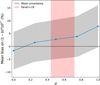 |
Fig. C.1 Evolution of the mean bias on the parameter combination |
![Mathematical equation: $\[(1-b)^{\alpha} 10^{Y^{*}}\]$](/articles/aa/full_html/2024/10/aa49513-24/aa49513-24-eq88.png)
Appendix D Representativity of the calibration samples
The Chandra-Planck sample used in this work contains 56 of the 71 clusters of the XMM-Newton-sample used by the Planck collaboration. Since six of the missing clusters are above the redshift limit of the Chandra sample, 56 of the 65 clusters of the XMM-Newton-sample that are below the redshift limit of the Chandra sample are included in the Chandra-Planck sample. To verify that the subset of the XMM-Newton-sample contained in the Chandra sample is representative of the full XMM-Newton sample, we compare mass and redshift distributions via Kolmogorov-Smirnov (KS) tests. We use XMM-Newton masses for all clusters and restrict the XMM-Newton sample to z<0.35 when comparing redshift distributions to not introduce a bias due to different ranges in the KS-test. Fig. D.1 presents the results of the KS tests: no indication of a different mass or redshift distribution is found. A final check is to calibrate the ![Mathematical equation: $\[Y_{\mathrm{SZ}}-M_{500}^{Y_{\mathrm{X}}}\]$](/articles/aa/full_html/2024/10/aa49513-24/aa49513-24-eq89.png) scaling relation with either the full XMM-Newton sample (expecting the same result as in Planck Collaboration XX 2014) or with the XMM-Newton sample restricted to clusters present in the Chandra-Planck sample. Fig. D.2 shows the scaling relations obtained for both samples. The difference in both intercept and slope is not statistically significant at around 0.3σ, meaning that the intersection sub-sample is not biased with respect to the full XMM-Newton sample in the
scaling relation with either the full XMM-Newton sample (expecting the same result as in Planck Collaboration XX 2014) or with the XMM-Newton sample restricted to clusters present in the Chandra-Planck sample. Fig. D.2 shows the scaling relations obtained for both samples. The difference in both intercept and slope is not statistically significant at around 0.3σ, meaning that the intersection sub-sample is not biased with respect to the full XMM-Newton sample in the ![Mathematical equation: $\[Y_{\mathrm{SZ}}-M_{500}^{Y_{\mathrm{X}}}\]$](/articles/aa/full_html/2024/10/aa49513-24/aa49513-24-eq90.png) plane. XMM-Newton derived masses were used in both cases and no redshift cut was applied when performing this comparison.
plane. XMM-Newton derived masses were used in both cases and no redshift cut was applied when performing this comparison.
Given the above results of the comparison between the intersection of the Chandra-Planck and XMM-Newton samples and the XMM-Newton sample, we conclude that the intersection is representative of the full XMM-Newton sample, and that we can thus compare the intersection with the Chandra sample and extrapolate the results to the full XMM-Newton sample. This extrapolation is required as we need to have X-ray data from the same instrument, in order to be able to draw conclusions from sample comparisons.
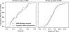 |
Fig. D.1 Comparison of the redshift and mass distribution of the XMM-Newton sample (in blue) with the Chandra-XMM-Newton intersection sample (in red). The p-value obtained when performing a KS-test comparing the two distributions is reported above each plot. |
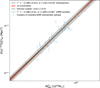 |
Fig. D.2 Comparison of the scaling relation obtained with the XMM-Newton sample restricted to the intersection (black line with uncertainty and intrinsic scatter) and the relation obtained with the full XMM-Newton sample (green line). |
To assess whether the XMM-Newton calibration sample used in Planck Collaboration XX (2014) and Planck Collaboration XXIV (2016) is representative of the cosmological sample on which the scaling relation is applied, we first compare the mass and redshift distributions of the XMM-Newton calibration sample, the Chandra calibration sample, and the full Planck cosmological sample. Given the limitations of the KS-test, we apply a z<0.35 cut when comparing redshift distributions. Since we want to compare how representative of the full cosmology sample the calibration samples are, no redshift cut is applied when studying mass distributions.
Fig. D.3 shows the results of the comparisons. The KS-tests do not point to significant differences between the redshift distributions of the calibration samples and the cosmology sample, although the Chandra calibration sample contains more low-redshift clusters even after restricting all samples to z<0.35. In terms of mass distribution, the comparisons show that both calibration samples are biased towards higher masses than the cosmology sample, with the bias being much stronger in the case of the XMM-Newton sample (p-value<0.0005 vs p-value=0.345). In the case of the Chandra-Planck sample, both of those differences are expected, since the ESZ and Cosmology samples are signal-to-noise limited with the same cut, but the ESZ sample was obtained on a noisier map, therefore requiring higher signal and ultimately more massive/less distant clusters. The bias of the XMM-Newton sample towards higher masses is also expected, since it is a compilation of pre-existing XMM-Newton observations, which are more likely to be targeted towards bright and massive clusters, as well as having a higher SZ signal-to-noise cut (7 as opposed to 6 for the cosmology sample).
The next, and arguably more important test, is to see if the XMM-Newton calibration sample is biased in the ![Mathematical equation: $\[Y_{\mathrm{SZ}}-M_{500}^{Y_{\mathrm{X}}}\]$](/articles/aa/full_html/2024/10/aa49513-24/aa49513-24-eq91.png) plane compared to an SZ-selected sample. Fig. D.4 shows the scaling relation obtained with the Chandra calibration sample restricted to the 56 clusters present in both Chandra and XMM-Newton samples (left panel), and the relation obtained with the Chandra calibration sample restricted to the 110 clusters present in the Chandra sample and absent from the XMM-Newton sample (right panel), and compares them to the scaling relation calibrated in this work on the full Chandra sample. As previously discussed, we need to use the intersection of the Chandra and XMM-Newton samples instead of the full XMM-Newton sample, since we need to have X-ray data from the same instrument in order to be able to draw conclusions from sample comparisons. We showed in the previous paragraph that the intersection of the Chandra and XMM-Newton samples is representative of the full XMM-Newton sample, and we can thus extrapolate the results obtained with the intersection to the full XMM-Newton sample. Although not very significant (respectively 0.7σ and 1σ), the scaling relation obtained with the intersection of the Chandra and XMM-Newton samples (respectively the exclusion of the XMM-Newton sample) has a lower (respectively higher) normalisation than the one obtained with the full Chandra sample. This means that, as could be expected, the XMM-Newton sample is slightly biased towards X-ray bright clusters, when compared to the SZ-selected Chandra sample.
plane compared to an SZ-selected sample. Fig. D.4 shows the scaling relation obtained with the Chandra calibration sample restricted to the 56 clusters present in both Chandra and XMM-Newton samples (left panel), and the relation obtained with the Chandra calibration sample restricted to the 110 clusters present in the Chandra sample and absent from the XMM-Newton sample (right panel), and compares them to the scaling relation calibrated in this work on the full Chandra sample. As previously discussed, we need to use the intersection of the Chandra and XMM-Newton samples instead of the full XMM-Newton sample, since we need to have X-ray data from the same instrument in order to be able to draw conclusions from sample comparisons. We showed in the previous paragraph that the intersection of the Chandra and XMM-Newton samples is representative of the full XMM-Newton sample, and we can thus extrapolate the results obtained with the intersection to the full XMM-Newton sample. Although not very significant (respectively 0.7σ and 1σ), the scaling relation obtained with the intersection of the Chandra and XMM-Newton samples (respectively the exclusion of the XMM-Newton sample) has a lower (respectively higher) normalisation than the one obtained with the full Chandra sample. This means that, as could be expected, the XMM-Newton sample is slightly biased towards X-ray bright clusters, when compared to the SZ-selected Chandra sample.
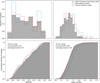 |
Fig. D.3 Comparison of the redshift (left side) and mass (right side) distributions of the XMM-Newton sample (in blue) and the Chandra sample (in red) with the Planck cosmology sample. The p-values obtained when performing a KS-test comparing each calibration sample with the cosmology sample is reported in the bottom panels. |
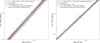 |
Fig. D.4 Scaling relations obtained when including or excluding clusters of the XMM-Newton sample. Left: Comparison of the scaling relation obtained with the Chandra sample restricted to the 56 clusters present in both Chandra and XMM-Newton samples (black line with uncertainty and intrinsic scatter) and the relation obtained with the full Chandra sample (green line). Right: Comparison of the scaling relation obtained with the Chandra sample restricted to the 110 clusters present in the Chandra sample and absent from the XMM-Newton sample (black line with uncertainty and intrinsic scatter) and the relation obtained with the full Chandra sample (green line). |
Appendix E Comparison of MMF algorithms
As mentioned in Sect. 2.5, the extraction of the SZ signal from the Planck maps using fixed positions and apertures from the X-ray data was done in Andrade-Santos et al. (2021) and in this work using fully independently developed MMF algorithms. Fig. E.1 shows the comparison of the YSZ measurements obtained in both works. The agreement is very good, with no departure from unity in both the slope and intercept of the best-fit relation. The intrinsic scatter around the best fit is also very low at 1%. For reference, this intrinsic scatter is better than the one obtained when comparing the results of MMF1 and MMF3 algorithms in Planck Collaboration XXVII (2016), which is around 3%. We are therefore confident that the YSZ measurements obtained in this work are robust.
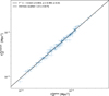 |
Fig. E.1 Comparison of YSZ obtained in this work and in Andrade-Santos et al. 2021, with the same X-ray derived positions and aperture as input, but independently developed MMF methods. |
Appendix F Full triangle plot of MCMC fitting
Fig. F.1 shows the full parameter constraints of the MCMC fitting of the number counts.
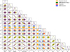 |
Fig. F.1 Parameter constraints obtained from the MCMC fitting of the number counts, for all cases considered in this work. |
References
- Abbott, T., Aguena, M., Alarcon, A., et al. 2020, Phys. Rev. D, 102, 023509 [NASA ADS] [CrossRef] [Google Scholar]
- Aiola, S., Calabrese, E., Maurin, L., et al. 2020, JCAP, 2020, 047 [Google Scholar]
- Akritas, M. G., & Bershady, M. A. 1996, ApJ, 470, 706 [Google Scholar]
- Alam, S., Ata, M., Bailey, S., et al. 2017, MNRAS, 470, 2617 [Google Scholar]
- Allen, S. W., Evrard, A. E., & Mantz, A. B. 2011, ARA&A, 49, 409 [Google Scholar]
- Amon, A., Gruen, D., Troxel, M. A., et al. 2022, Phys. Rev. D, 105, 023514 [NASA ADS] [CrossRef] [Google Scholar]
- Andrade-Santos, F., Pratt, G. W., Melin, J.-B., et al. 2021, ApJ, 914, 58 [NASA ADS] [CrossRef] [Google Scholar]
- Andreon, S. 2014, A&A, 570, L10 [NASA ADS] [CrossRef] [EDP Sciences] [Google Scholar]
- Arnaud, M., Pratt, G. W., Piffaretti, R., et al. 2010, A&A, 517, A92 [CrossRef] [EDP Sciences] [Google Scholar]
- Balkenhol, L., Dutcher, D., Mancini, A. S., et al. 2023, Phys. Rev. D, 108, 023510 [NASA ADS] [CrossRef] [Google Scholar]
- Battaglia, N., Leauthaud, A., Miyatake, H., et al. 2016, JCAP, 2016, 013 [NASA ADS] [CrossRef] [Google Scholar]
- Bleem, L. E., Stalder, B., de Haan, T., et al. 2015, ApJS, 216, 27 [Google Scholar]
- Bleem, L. E., Bocquet, S., Stalder, B., et al. 2020, ApJS, 247, 25 [Google Scholar]
- Bleem, L. E., Klein, M., Abbott, T. M. C., et al. 2024, Open J. Astrophys., 7, 13 [CrossRef] [Google Scholar]
- Bocquet, S., Dietrich, J. P., Schrabback, T., et al. 2019, ApJ, 878, 55 [Google Scholar]
- Bocquet, S., Grandis, S., Bleem, L. E., et al. 2023, SPT Clusters with DES and HST Weak Lensing. I. Cluster Lensing and Bayesian Population Modeling of Multi-Wavelength Cluster Datasets, Phys. Rev. D., submitted [arXiv:2310.12213] [Google Scholar]
- Bocquet, S., Grandis, S., Bleem, L. E., et al. 2024, SPT Clusters with DES and HST Weak Lensing. II. Cosmological Constraints from the Abundance of Massive Halos, Phys. Rev. D., submitted [arXiv:2401.02075] [Google Scholar]
- Bonamente, M. 2020, J. Appl. Stat., 47, 2044 [NASA ADS] [CrossRef] [Google Scholar]
- Böss, L. M., Steinwandel, U. P., Dolag, K., & Lesch, H. 2022, MNRAS, 519, 548 [CrossRef] [Google Scholar]
- Costanzi, M., Saro, A., Bocquet, S., et al. 2021, Phys. Rev. D, 103, 043522 [Google Scholar]
- Dalal, R., Li, X., Nicola, A., et al. 2023, Phys. Rev. D, 108, 123519 [CrossRef] [Google Scholar]
- Dolag, K., & Schindler, S. 2000, A&A, 364, 491 [NASA ADS] [Google Scholar]
- Farahi, A., Mulroy, S. L., Evrard, A. E., et al. 2019, Nat. Commun., 10, 2504 [NASA ADS] [CrossRef] [Google Scholar]
- Garrel, C., Pierre, M., Valageas, P., et al. 2022, A&A, 663, A3 [NASA ADS] [CrossRef] [EDP Sciences] [Google Scholar]
- Ghirardini, V., Bulbul, E., Artis, E., et al. 2024, A&A, 689, A298 [NASA ADS] [CrossRef] [EDP Sciences] [Google Scholar]
- Gianfagna, G., De Petris, M., Yepes, G., et al. 2021, MNRAS, 502, 5115 [NASA ADS] [CrossRef] [Google Scholar]
- Gouin, C., Bonnaire, T., & Aghanim, N. 2021, A&A, 651, A56 [NASA ADS] [CrossRef] [EDP Sciences] [Google Scholar]
- Gouin, C., Gallo, S., & Aghanim, N. 2022, A&A, 664, A198 [NASA ADS] [CrossRef] [EDP Sciences] [Google Scholar]
- Grandis, S., Ghirardini, V., Bocquet, S., et al. 2024, A&A, 687, A178 [NASA ADS] [CrossRef] [EDP Sciences] [Google Scholar]
- Henry, J. P. 1997, ApJ, 489, L1 [NASA ADS] [CrossRef] [Google Scholar]
- Herbonnet, R., Sifón, C., Hoekstra, H., et al. 2020, MNRAS, 497, 4684 [NASA ADS] [CrossRef] [Google Scholar]
- Herranz, D., Sanz, J. L., Barreiro, R. B., & Martinez-Gonzalez, E. 2002, ApJ, 580, 610 [CrossRef] [Google Scholar]
- Heymans, C., Tröster, T., Asgari, M., et al. 2021, A&A, 646, A140 [NASA ADS] [CrossRef] [EDP Sciences] [Google Scholar]
- Hilton, M., Sifón, C., Naess, S., et al. 2021, ApJS, 253, 3 [Google Scholar]
- Hoekstra, H., Mahdavi, A., Babul, A., & Bildfell, C. 2012, MNRAS, 427, 1298 [NASA ADS] [CrossRef] [Google Scholar]
- Hoekstra, H., Herbonnet, R., Muzzin, A., et al. 2015, MNRAS, 449, 685 [NASA ADS] [CrossRef] [Google Scholar]
- Kelly, B. C. 2007, ApJ, 665, 1489 [Google Scholar]
- Klein, M., Mohr, J. J., Bocquet, S., et al. 2024, MNRAS, 531, 3973 [NASA ADS] [CrossRef] [Google Scholar]
- Kravtsov, A., & Borgani, S. 2012, ARA&A, 50, 353 [NASA ADS] [CrossRef] [Google Scholar]
- Kravtsov, A. V., Vikhlinin, A., & Nagai, D. 2006, ApJ, 650, 128 [Google Scholar]
- Lesci, G. F., Marulli, F., Moscardini, L., et al. 2022, A&A, 659, A88 [NASA ADS] [CrossRef] [EDP Sciences] [Google Scholar]
- Lewis, A. 2019, arXiv e-prints [arXiv:1910.13970] [Google Scholar]
- Lewis, A., & Bridle, S. 2002, Phys. Rev. D, 66, 103511 [Google Scholar]
- Li, X., Zhang, T., Sugiyama, S., et al. 2023, Phys. Rev. D, 108, 123518 [CrossRef] [Google Scholar]
- Lovisari, L., Forman, W. R., Jones, C., et al. 2017, ApJ, 846, 51 [Google Scholar]
- Madhavacheril, M. S., Qu, F. J., Sherwin, B. D., et al. 2024, ApJ, 962, 113 [CrossRef] [Google Scholar]
- Melin, J.-B., & Bartlett, J. G. 2015, A&A, 578, A21 [NASA ADS] [CrossRef] [EDP Sciences] [Google Scholar]
- Melin, J.-B., Bartlett, J. G., & Delabrouille, J. 2006, A&A, 459, 341 [NASA ADS] [CrossRef] [EDP Sciences] [Google Scholar]
- Miyatake, H., Sugiyama, S., Takada, M., et al. 2023, Phys. Rev. D, 108, 123517 [NASA ADS] [CrossRef] [Google Scholar]
- Murray, S. G., Power, C., & Robotham, A. S. G. 2013, Astron. Comput., 3–4, 23 [CrossRef] [Google Scholar]
- Pearce, F. A., Kay, S. T., Barnes, D. J., Bower, R. G., & Schaller, M. 2020, MNRAS, 491, 1622 [NASA ADS] [CrossRef] [Google Scholar]
- Planck Collaboration VIII. 2011, A&A, 536, A8 [NASA ADS] [CrossRef] [EDP Sciences] [Google Scholar]
- Planck Collaboration XI. 2011, A&A, 536, A11 [NASA ADS] [CrossRef] [EDP Sciences] [Google Scholar]
- Planck Collaboration XVI. 2014, A&A, 571, A16 [NASA ADS] [CrossRef] [EDP Sciences] [Google Scholar]
- Planck Collaboration XX. 2014, A&A, 571, A20 [NASA ADS] [CrossRef] [EDP Sciences] [Google Scholar]
- Planck Collaboration XXIX. 2014, A&A, 571, A29 [NASA ADS] [CrossRef] [EDP Sciences] [Google Scholar]
- Planck Collaboration XXIV. 2016, A&A, 594, A24 [NASA ADS] [CrossRef] [EDP Sciences] [Google Scholar]
- Planck Collaboration XXVII. 2016, A&A, 594, A27 [NASA ADS] [CrossRef] [EDP Sciences] [Google Scholar]
- Planck Collaboration VI. 2020, A&A, 641, A6 [NASA ADS] [CrossRef] [EDP Sciences] [Google Scholar]
- Planck Collaboration Int. XLVI. 2016, A&A, 596, A107 [NASA ADS] [CrossRef] [EDP Sciences] [Google Scholar]
- Potter, C., Tümer, A., Wang, Q. H. S., et al. 2023, ApJ, 958, 112 [NASA ADS] [CrossRef] [Google Scholar]
- Pratt, G. W., Arnaud, M., Biviano, A., et al. 2019, Space Sci. Rev., 215, 25 [Google Scholar]
- Rasia, E., Tormen, G., & Moscardini, L. 2004, MNRAS, 351, 237 [NASA ADS] [CrossRef] [Google Scholar]
- Rasia, E., Ettori, S., Moscardini, L., et al. 2006, MNRAS, 369, 2013 [CrossRef] [Google Scholar]
- Rozo, E., Wechsler, R. H., Rykoff, E. S., et al. 2010, ApJ, 708, 645 [Google Scholar]
- Salvati, L., Douspis, M., Ritz, A., Aghanim, N., & Babul, A. 2019, A&A, 626, A27 [NASA ADS] [CrossRef] [EDP Sciences] [Google Scholar]
- Sand, D. J., Graham, M. L., Bildfell, C., et al. 2011, ApJ, 729, 142 [Google Scholar]
- Sand, D. J., Graham, M. L., Bildfell, C., et al. 2012, ApJ, 746, 163 [NASA ADS] [CrossRef] [Google Scholar]
- Schellenberger, G., Reiprich, T. H., Lovisari, L., Nevalainen, J., & David, L. 2015, A&A, 575, A30 [NASA ADS] [CrossRef] [EDP Sciences] [Google Scholar]
- Sereno, M., & Ettori, S. 2017, MNRAS, 468, 3322 [CrossRef] [Google Scholar]
- Steigman, G. 2008, arXiv e-prints [arXiv:0807.3004] [Google Scholar]
- Sugiyama, S., Miyatake, H., More, S., et al. 2023, Phys. Rev. D, 108, 123521 [NASA ADS] [CrossRef] [Google Scholar]
- Sunyaev, R. A., & Zeldovich, Y. B. 1972, Comments on Astrophys. Space Phys., 4, 173 [Google Scholar]
- Tinker, J., Kravtsov, A. V., Klypin, A., et al. 2008, Astrophys. J., 688, 709 [CrossRef] [Google Scholar]
- Vikhlinin, A., Markevitch, M., Murray, S. S., et al. 2005, ApJ, 628, 655 [Google Scholar]
- Vikhlinin, A., Kravtsov, A., Forman, W., et al. 2006, ApJ, 640, 691 [Google Scholar]
- Vikhlinin, A., Burenin, R. A., Ebeling, H., et al. 2009a, ApJ, 692, 1033 [Google Scholar]
- Vikhlinin, A., Kravtsov, A. V., Burenin, R. A., et al. 2009b, ApJ, 692, 1060 [Google Scholar]
- Von Der Linden, A., Mantz, A., Allen, S. W., et al. 2014, MNRAS, 443, 1973 [NASA ADS] [CrossRef] [Google Scholar]
- Watson, W. A., Iliev, I. T., D’Aloisio, A., et al. 2013, MNRAS, 433, 1230 [Google Scholar]
- White, S. D. M., Navarro, J. F., Evrard, A. E., & Frenk, C. S. 1993, Nature, 366, 429 [Google Scholar]
- Wicker, R., Douspis, M., Salvati, L., & Aghanim, N. 2023, A&A, 674, A48 [NASA ADS] [CrossRef] [EDP Sciences] [Google Scholar]
All Tables
YSZ − M500 scaling relations with free redshift dependence for both calibration samples.
All Figures
|
Fig. 1 Mass-redshift distribution of the Chandra-Planck sample, the Planck MMF3 cosmological sample, and the XMM-Newton calibration sample used by the Planck collaboration. |
| In the text | |
|
Fig. 2 Calibration of the |
| In the text | |
|
Fig. 3 Hydrostatic mass bias determination for Chandra scaling relation, with selection bias accounted for. The clusters detected by Planck are plotted in blue, while the orange points are the mass upper limits for the non-detected clusters. The black line shows the best-fit relation, with red contours corresponding to 1σ uncertainties, and grey contours to the intrinsic scatter. |
| In the text | |
|
Fig. 4 Mass distributions of the clusters of the full Planck cosmological sample, when using the Planck 2015 scaling relation in blue and the relation calibrated in this work in red. The distributions in both panels are obtained from the same sample and identical SZ data. Left: hydrostatic masses i.e. not including a (1 − b) correcting factor, as obtained from Eq. (7). Right: ‘true’ masses, obtained from the full scaling relations including the bias corrections presented in Table 1: |
| In the text | |
|
Fig. 5 Final cosmological constraints obtained with the scaling relation calibrated in Sect. 3 (in red) and comparison with constraints from SZ number counts obtained in Planck Collaboration XXIV (2016) (in yellow), constraints from CMB primary anisotropies from Planck Collaboration VI (2020) (in green), and constraints obtained using the scaling relation from Planck Collaboration XXIV (2016) with the bias calibrated in Sect. 3.2 (in blue). |
| In the text | |
|
Fig. 6 Retrieved YSZ − M500 scaling relation on 100 synthetic calibration samples compared with the true underlying relation used for sample generation. The retrieved slope (divided by three for better readability) is shown in blue, the retrieved intrinsic scatter in green, and the relevant combination of the degenerated parameters (1 − b) and Y* in red. The true value of each parameter is shown by the black dashed lines and the mean uncertainty returned by the calibration procedure is shown by the grey contours. |
| In the text | |
|
Fig. 7 Calibration of the |
| In the text | |
|
Fig. 8 Calibration of the YSZ − scaling relation, letting the redshift dependence vary as a free parameter. The high and low redshift subsamples are shown in different colours to help visualise the effect of the free redshift dependence, but the fit is performed on the whole sample at once. The black line shows the best-fit relation, with red contours corresponding to 1σ uncertainties, and grey contours to the intrinsic scatter. |
| In the text | |
|
Fig. 9 Cosmological constraints obtained with the redshift dependence fitted from the data, with both Chandra (in red) and XMM-Newton (in blue) calibration samples, and comparison with the results obtained with the fixed, self-similar redshift dependence using the Chandra calibration sample (in yellow) and Planck Collaboration VI (2020) constraints from CMB primary anisotropies (in green). |
| In the text | |
|
Fig. 10 Redshift (top panel) and signal-to-noise (bottom panel) distribution of best-fit models from the four analysis cases presented in this work. The observed counts in the PSZ2 catalogue (q > 6) are plotted as the black points. |
| In the text | |
|
Fig. 11 Comparison of the S8 constraints obtained in this work (in bold) with other recent analyses. |
| In the text | |
|
Fig. A.1 100 samples taken at random from the MCMC mass estimation procedure of the PSZ2 G033.97-76.61 cluster plotted over the 2D probability map from the MMF3 detection found in the PSZ2 catalogue. |
| In the text | |
|
Fig. B.1 Final cosmological constraints obtained with the bias calculated not including the non-detections (in green) or taking them into account (in red). |
| In the text | |
|
Fig. C.1 Evolution of the mean bias on the parameter combination |
| In the text | |
|
Fig. D.1 Comparison of the redshift and mass distribution of the XMM-Newton sample (in blue) with the Chandra-XMM-Newton intersection sample (in red). The p-value obtained when performing a KS-test comparing the two distributions is reported above each plot. |
| In the text | |
|
Fig. D.2 Comparison of the scaling relation obtained with the XMM-Newton sample restricted to the intersection (black line with uncertainty and intrinsic scatter) and the relation obtained with the full XMM-Newton sample (green line). |
| In the text | |
|
Fig. D.3 Comparison of the redshift (left side) and mass (right side) distributions of the XMM-Newton sample (in blue) and the Chandra sample (in red) with the Planck cosmology sample. The p-values obtained when performing a KS-test comparing each calibration sample with the cosmology sample is reported in the bottom panels. |
| In the text | |
|
Fig. D.4 Scaling relations obtained when including or excluding clusters of the XMM-Newton sample. Left: Comparison of the scaling relation obtained with the Chandra sample restricted to the 56 clusters present in both Chandra and XMM-Newton samples (black line with uncertainty and intrinsic scatter) and the relation obtained with the full Chandra sample (green line). Right: Comparison of the scaling relation obtained with the Chandra sample restricted to the 110 clusters present in the Chandra sample and absent from the XMM-Newton sample (black line with uncertainty and intrinsic scatter) and the relation obtained with the full Chandra sample (green line). |
| In the text | |
|
Fig. E.1 Comparison of YSZ obtained in this work and in Andrade-Santos et al. 2021, with the same X-ray derived positions and aperture as input, but independently developed MMF methods. |
| In the text | |
|
Fig. F.1 Parameter constraints obtained from the MCMC fitting of the number counts, for all cases considered in this work. |
| In the text | |
Current usage metrics show cumulative count of Article Views (full-text article views including HTML views, PDF and ePub downloads, according to the available data) and Abstracts Views on Vision4Press platform.
Data correspond to usage on the plateform after 2015. The current usage metrics is available 48-96 hours after online publication and is updated daily on week days.
Initial download of the metrics may take a while.