| Issue |
A&A
Volume 689, September 2024
|
|
|---|---|---|
| Article Number | A195 | |
| Number of page(s) | 14 | |
| Section | The Sun and the Heliosphere | |
| DOI | https://doi.org/10.1051/0004-6361/202450769 | |
| Published online | 12 September 2024 | |
Propagating kink waves in an open coronal magnetic flux tube with gravitational stratification: Magnetohydrodynamic simulation and forward modelling
1
School of Earth and Space Sciences, Peking University, Beijing 100871, PR China
2
Centre for mathematical Plasma-Astrophysics, Department of Mathematics, KU Leuven, Celestijnenlaan 200B Bus 2400, 3001 Leuven, Belgium
3
Shandong Provincial Key Laboratory of Optical Astronomy and Solar-Terrestrial Environment, Institute of Space Sciences, Shandong University, Weihai 264209, China
Received:
17
May
2024
Accepted:
26
June
2024
Abstract
Context. In coronal open-field regions, such as coronal holes, there are many transverse waves propagating along magnetic flux tubes, which are generally interpreted as kink waves. Previous studies have highlighted their potential role in coronal heating, solar wind acceleration, and seismological diagnostics of various physical parameters.
Aims. This study aims to investigate propagating kink waves, considering both vertical and horizontal density inhomogeneity, using 3D magnetohydrodynamic (MHD) simulations.
Methods. We established a 3D MHD model of a gravitationally stratified open flux tube, incorporating a velocity driver at the lower boundary to excite propagating kink waves. Forward modelling was conducted to synthesise observational signatures of the Fe IX 17.1 nm line.
Results. Resonant absorption and density stratification both affect the wave amplitude. When diagnosing the relative density profile with velocity amplitude, resonant damping needs to be properly considered to avoid a possible underestimation. In addition, unlike standing modes, propagating waves are believed to be Kelvin-Helmholtz stable. In the presence of vertical stratification, however, the phase mixing of transverse motions around the tube boundary can still induce small-scale structures, partially dissipating wave energy and leading to a temperature increase, especially at higher altitudes. Moreover, we conducted forward modeling to synthesise observational signatures, which revealed the promising potential of future coronal imaging spectrometers such as MUSE in resolving these wave-induced signatures. Also, the synthesised intensity signals exhibit apparent periodic variations, offering a potential method for indirectly observing propagating kink waves with current extreme ultraviolet imagers.
Key words: methods: numerical / Sun: atmosphere / Sun: corona / Sun: oscillations
Corresponding authors; This email address is being protected from spambots. You need JavaScript enabled to view it. , This email address is being protected from spambots. You need JavaScript enabled to view it. .
© The Authors 2024
 Open Access article, published by EDP Sciences, under the terms of the Creative Commons Attribution License (https://creativecommons.org/licenses/by/4.0), which permits unrestricted use, distribution, and reproduction in any medium, provided the original work is properly cited.
This article is published in open access under the Subscribe to Open model. This email address is being protected from spambots. You need JavaScript enabled to view it. to support open access publication.
1. Introduction
In the past two decades, propagating transverse motions have frequently been detected in the solar corona (see the reviews by Banerjee et al. 2021; Morton et al. 2023). These waves are commonly interpreted as kink waves (Van Doorsselaere et al. 2008; Goossens et al. 2009). Observations have revealed their ubiquitous presence in the solar corona (e.g. Tomczyk et al. 2007; Tomczyk & McIntosh 2009), and show they carry substantial energy flux that could potentially contribute to coronal heating and solar wind acceleration (e.g. Banerjee et al. 2009; Hahn et al. 2012; McIntosh et al. 2011). Another important application of these waves is in coronal seismology. For instance, with the propagating kink waves observed by the Coronal Multichannel Polarimeter (CoMP; Tomczyk et al. 2008), global maps of the coronal magnetic field can be obtained (Yang et al. 2020a,b), marking a significant advancement towards routine measurements of the coronal magnetic field. Therefore, propagating kink waves are of great significance in solar physics research.
In general, kink waves primarily manifest as propagating modes in open-field regions or some large closed magnetic structures (i.e. coronal loops), while manifesting as standing modes in relatively small coronal loops in both quiet-Sun and active regions (Nakariakov et al. 1999; Aschwanden et al. 1999; Tian et al. 2012; Nisticò et al. 2013; Anfinogentov et al. 2015; Goddard et al. 2016; Gao et al. 2022; Li & Long 2023; Petrova et al. 2023). How and why these transverse waves appear differently in coronal loops of varying sizes is not clear (see e.g. Threlfall et al. 2013; Long et al. 2017; Morton et al. 2021; Tiwari et al. 2021; Skirvin et al. 2023; Gao et al. 2023; Li et al. 2023). In this paper we focus on kink waves in open-field coronal regions, for example coronal holes, where the propagating modes naturally predominate. The typical structures or wave guides here are plumes, characterised by a thin, long ray-like appearance (see the review by Poletto 2015).
In observations, kink waves propagating along plumes or coronal open flux tubes can be studied using spectroscopic observations or extreme ultraviolet (EUV) image sequences. On one hand, spectroscopic observations are mainly based on the CoMP Fe XIII 1074.7 nm emission line, which can show the existence of persistent Doppler velocity fluctuations distributing nearly everywhere in the off-limb corona (Tomczyk et al. 2007; Tomczyk & McIntosh 2009; Yang et al. 2020a,b). Based on the wave-tracking method, the propagating speed or phase speed has been estimated to be 300−700 km s−1. In the open-field coronal hole regions, the Fe XIII 1074.7 nm line normally has a low signal-to-noise ratio. Nevertheless, some authors still managed to detect signals of propagating kink motions with a velocity amplitude of several kilometres per second (Liu et al. 2015; Morton et al. 2015). Similar signatures were also captured by Mancuso & Raymond (2015) with H I Ly α coronal emission line profiles. Morton et al. (2015) also revealed the existence of downward propagating waves, with a decreased power compared with that of upward propagating ones. On the other hand, EUV imaging observations with a high spatial and temporal resolution provide us with another approach to investigating transverse waves in open-field regions through the plane-of-sky (POS) displacements of magnetised plasma structures such as plumes (McIntosh et al. 2011; Thurgood et al. 2014; Morton et al. 2015; Weberg et al. 2018, 2020). Most previous EUV observations used the data from the Atmospheric Imaging Assembly (AIA; Lemen et al. 2012) on board the Solar Dynamics Observatory (SDO; Pesnell et al. 2012). Comparisons between imaging and spectroscopic observation results can be found in Morton et al. (2015, 2019). Their observations show a peak at ∼3.5 mHz in the velocity power spectrum (see Figure 1d in Morton et al. 2019), suggesting a connection with photospheric p-mode leakage (see also Tomczyk & McIntosh 2009; Weberg et al. 2020; Gao et al. 2022, 2023). Spectroscopic analysis has also shown variations in the non-thermal line broadening, which could be interpreted as the signature of Alfvén waves (e.g. Banerjee et al. 1998, 2009; Doschek et al. 2007; Jess et al. 2009; Hahn et al. 2012). However, such an interpretation remains a subject of debate because the line broadening could be attributed to other effects, such as flow inhomogeneities along the line of sight (LOS) or sausage modes (see e.g. Tian et al. 2011, 2014; Mathioudakis et al. 2013; Zhu et al. 2023). Direct observations of torsional Alfvén waves in the coronal open-field regions are still lacking (cf., Kohutova et al. 2020; Petrova et al. 2024). Therefore, here we restricted the observed transverse waves to kink waves only (see Van Doorsselaere et al. 2008; Goossens et al. 2009, 2012).
The propagation of kink waves in the magnetised, inhomogeneous coronal medium is influenced by two primary factors. Firstly, the amplitude increases with height due to decreasing density. Assuming that the wave damping or dissipation is relatively weak, the energy flux would be nearly constant:  , where ⟨ρ⟩ represents the average density, vamp the velocity amplitude, and ck the local kink speed (phase speed), defined as
  , with μ0 representing the magnetic permeability (e.g. Tomczyk & McIntosh 2009; Morton et al. 2015; Yang et al. 2020b; Bate et al. 2022). Thus, if the magnetic field, B(z), changes only slightly, the decrease in density with height can result in an amplification of the wave amplitude (Banerjee et al. 1998, 2009; Soler et al. 2011; Morton et al. 2012; Morton 2014; van Ballegooijen et al. 2014; Weberg et al. 2020). The second factor involves the resonant damping of the kink waves (e.g. Terradas et al. 2010; Verth et al. 2010; Pascoe et al. 2010, 2011, 2012). The damping arises from the inhomogeneity across the loop, transferring energy from the bulk transverse oscillations to azimuthal motions in the boundary layer. Subsequently, the energy can be dissipated through phase mixing (Heyvaerts & Priest 1983; Soler & Terradas 2015; Pagano & De Moortel 2017; Howson et al. 2020) and the development of Kelvin-Helmholtz instability (KHI; see Pagano & De Moortel 2019). Other effects such as uniturbulence may also contribute to wave dissipation (Magyar et al. 2017, 2019; Van Doorsselaere et al. 2020).
While the joint influence of these two effects on propagating kink waves has been analytically investigated in Soler et al. (2011), detailed studies with 3D magnetohydrodynamic (MHD) simulations and taking both vertical and horizontal inhomogeneities into account have been rare. A few previous numerical investigations (Pascoe et al. 2010, 2011, 2012, 2015; De Moortel & Pascoe 2012; De Moortel et al. 2016; Magyar et al. 2017; Pagano & De Moortel 2017, 2019; Pagano et al. 2020; Howson et al. 2020; Fyfe et al. 2021; Meringolo et al. 2024) focused on the damping mechanism and heating contribution of these waves without considering vertical density stratification, which can be important as it can amplify the amplitude and thus affect the wave damping or dissipation. The varying density also influences the estimation of the wave energy flux and total radiative loss. On the other hand, studies incorporating density variation along the magnetic field usually neglect the density inhomogeneity across the field (e.g. van Ballegooijen et al. 2014; Matsumoto 2018; Pant & Van Doorsselaere 2020; Pascoe et al. 2022), and consequently, the resonant absorption and phase mixing are either not present or not effective. Recently, Pant et al. (2019) and Sen & Pant (2021) established models with multiple density-enhanced flux tubes and gravitational stratification. However, after kink waves are excited, these oscillating tubes quickly interact with each other and generate (uni)turbulence, making it impossible to investigate the wave behaviour of one single flux tube in detail. Additionally, Pelouze et al. (2023) built up a single flux tube model with stratification, but only focused on the cutoff effect at the lower atmosphere rather than the coronal part.
In this study we report results from a detailed investigation of the propagating kink waves in open coronal magnetic flux tubes (or plumes) perpendicular to the solar surface with 3D MHD simulations. Both horizontal inhomogeneity and vertical stratification were considered to better reflect a realistic case. We also performed forward modelling to synthesise the observational signatures of these waves. The paper is organised as follows: In Section 2 we describe our simulation setup and methodology. Section 3 and 4 present the simulation and forward modelling results, respectively. We further discuss our results in Section 5 and summarise our findings in Section 6.
2. Method
In this study we aim to model a plume in the coronal open-field region as a magnetic flux tube in 3D MHD simulations. The length, L, of the tube was chosen to be 150 Mm along the z axis in Cartesian coordinates. We included a gravity along the tube specified as
 (1)
(1)
to reflect the stratification, where R⊙ is the solar radius, g0 = 274 m s−2 is the gravity at the solar surface (or, approximately, at the base of the corona). The lower solar atmosphere was not considered in our model. Thus, we adopted a uniform temperature as T = 1 MK.
At the lower boundary, the horizontal density profile was set as
![Mathematical equation: $$ \begin{aligned} \rho (x,y,z=0)=\rho _{\rm e}+\frac{(\rho _{\rm i}-\rho _{\rm e})}{2}\left\{ 1-\tanh \left[\left(\frac{\sqrt{x^2+y^2}}{R}-1\right)b\right]\right\} . \end{aligned} $$](/articles/aa/full_html/2024/09/aa50769-24/aa50769-24-eq4.gif) (2)
(2)
The external and internal densities are set to be ρe = 2.5 × 10⁻¹⁵ g cm−3, and ρi = 7.5 × 10⁻¹⁵ g cm−3, respectively, resulting in a density contrast (ζ = ρi/ρe) of 3 (e.g. Verwichte et al. 2013; Morton et al. 2021). The tube radius R and the dimensionless constant b were set to be 1 Mm and 8, resulting in a boundary layer with a width of l ∼ 0.6R = 0.6 Mm. The density at larger heights was integrated layer by layer to satisfy the field-aligned hydrostatic equilibrium with a finite difference scheme as described in Pelouze et al. (2023), Guo et al. (2023a, 2023) and Karampelas & Van Doorsselaere (2024). The horizontal and vertical profiles of density in the initial state are shown with black lines in Figures 1b and d.
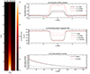 |
Fig. 1. Illustration of the model setup. (a) Density distribution at the y = 0 plane after relaxation. (b) and (c) Horizontal profiles of the density and magnetic field along the x axis at three different heights (indicated by different line styles). (d) Vertical profile of the density, demonstrating gravitational stratification, with solid and dashed lines indicating density within and outside the flux tube, respectively. The black and red lines in panels b–d represent states before and after relaxation, respectively. We note that the magnetic field in the initial state (before relaxation) is uniform along the z axis, and hence there is only one black line in panel c. |
The magnetic field was initially set to maintain total pressure balance at the lower boundary, with an internal strength of 10 G, as shown in Figure 1c. Constrained only in the z direction, the magnetic field exhibits zero gradients along the z axis to ensure ∇ ⋅ B = 0. Such an initial setup is not in magnetohydrostatic equilibrium, and thus a relaxation for 2400 s was conducted to reach total pressure balance at every height (see Pelouze et al. 2023; Guo et al. 2023a; Gao et al. 2023; Karampelas & Van Doorsselaere 2024). During the relaxation stage, we introduced a velocity absorption factor, α, to suppress initial velocity flows in the simulation domain and reflections from the upper boundary, defined as
![Mathematical equation: $$ \begin{aligned} {\tiny \alpha (z,t)=\left\{ \begin{aligned}&0.995,&t\le t_{0},\\&\left(0.995+0.005\times \frac{t-t_0}{t_0}\right)\left[1-(1-\alpha ^*(z)) \frac{t-t_0}{t_0}\right],&t_{0}<t\le 2t_{0},\\&\alpha ^*(z),&t> 2t_{0}. \end{aligned} \right.} \end{aligned} $$](/articles/aa/full_html/2024/09/aa50769-24/aa50769-24-eq5.gif) (3)
(3)
Here α*(z) describes the absorption factor in the final stage:
 (4)
(4)
The velocity was multiplied by α(z, t)≤1, and we set t0 and L0 to be 100 s and 100 Mm. The introduction of the factor is inspired by some previous studies (Pelouze et al. 2023; Guo et al. 2023a; Gao et al. 2023). The main difference here is that we set the upper 50 Mm (z > L0 = 100 Mm) as a permanent absorption layer to continuously suppress the reflection from the upper boundary (even after the relaxation stage). Figure 2 illustrates the distribution and evolution of α.
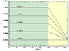 |
Fig. 2. Dependence of the velocity absorption factor, α, on height (z, horizontal axis) and time (indicated by different lines). Green and yellow shading distinguishes the regions below and above 100 Mm. The latter can be regarded as an extended upper boundary, and we only analysed and discuss the results below 100 Mm (green shading). |
After the relaxation, the horizontal velocities vx and vy remain negligible with a maximum value of 0.03 km s−1, while the vertical velocity vz can be gradually suppressed to less than 1.5 km s−1, much smaller than the velocity of the driven kink waves. Therefore, we regarded the relaxed state (achieved after 2400 s) as a quasi-magnetohydrostatic equilibrium. As shown in Figures 1b–d, the distributions of density and magnetic field only exhibit minor changes after relaxation (indicated by the red lines). The primary density change occurs near the base of the flux tube. A possible reason is that the vertical hydrostatic equilibrium in our initial setup is not completely accurate, resulting in a net downward mass flow. Additionally, the magnetic field inside the flux tube experiences a slight increase with height, which is in line with the expectation that at higher altitudes, the difference in internal and external thermal pressure diminishes, resulting in a decrease in the magnetic pressure difference. Furthermore, this change in the magnetic field can lead to an increase in magnetic pressure with height, creating an upward vertical gradient in the total pressure, which could also cause density to accumulate at the tube base. Finally, Figure 1a provides a direct visualisation of our model (post-relaxation) by illustrating the density profile at the y = 0 plane.
To excite propagating kink waves, we added a continuous velocity driver at the lower boundary (z = 0). The driver has a dipole-like velocity field, similar to Pascoe et al. (2010), Karampelas et al. (2017), and Guo et al. (2019). The velocity inside the tube has only the x component, given by
 (5)
(5)
and the velocity outside the tube is given by
![Mathematical equation: $$ \begin{aligned} \boldsymbol{v}(x,y)=v_0R^2\cos \left(\frac{2\pi t}{P}\right)\left[\frac{x^2-y^2}{(x^2+y^2)^2}{\boldsymbol{e}}_x+\frac{2xy}{(x^2+y^2)^2}{\boldsymbol{e}}_y\right], \end{aligned} $$](/articles/aa/full_html/2024/09/aa50769-24/aa50769-24-eq8.gif) (6)
(6)
where we adopted a velocity amplitude (v0) of 8 km s−1, and a period (P) of 300 s (see e.g. Tomczyk & McIntosh 2009; Weberg et al. 2018). For simplicity, here we only used a mono-period driver. We note that the propagating kink waves can be better simulated with a broad-band or multi-frequency driver (e.g. Pascoe et al. 2015; Magyar et al. 2017; Magyar & Van Doorsselaere 2018; Pagano & De Moortel 2019; Pant et al. 2019; Sen & Pant 2021). However, such a simplified driver can already satisfy the main purpose of this study, and the case with a broad-band driver will be explored in a future study.
The PLUTO code (Mignone et al. 2007) was utilised to solve the 3D time-dependent non-linear ideal MHD equations. We employed a second-order parabolic spatial scheme for time stepping and calculated numerical fluxes with a Roe Riemann solver. The radiative cooling, thermal conduction, explicit resistivity, and viscosity were not included during the simulation. We adopted the hyperbolic divergence cleaning method to maintain the divergence-free nature of the magnetic field. We chose not to use dimensionless parameters because using dimensional parameters allows for more intuitive comparisons with real observations. The computational domain spans [−4, 4] Mm × [−4, 4] Mm × [0, 150] Mm, with a uniform grid of 128 × 128 × 1024 cells, yielding resolutions of 62.5 km in the x and y directions, and 146.5 km in the z direction. Although the horizontal resolution could be relatively low compared to previous studies, the small-scale structures associated with resonant absorption and phase mixing can still form naturally in the tube boundary (see below). Such a low resolution also induces a large numerical resistivity ηn, which is roughly estimated to be of the order of 10−7 s (in CGS), further giving a magnetic Reynolds number of ∼2.8 × 10³. Since the numerical resistivity is much larger than the expected value of the solar corona and the magnetic Reynolds number is much lower (see Karampelas et al. 2017), we performed a convergence test by re-running the simulation with double horizontal resolution. The simulation results, such as temperature increase (see Section 3), only change mildly, and these changes do not affect our main conclusions.
For the boundary condition, we employed outflow conditions for all the lateral boundaries and the upper boundary (z = 150 Mm). During the relaxation stage, the lower boundary (z = 0) remained fixed with all velocities set to zero. Subsequently, we modified the velocity conditions according to Equation (5) to drive upward propagating kink waves. We also note that an outflow upper boundary cannot fully eliminate the reflective flows or waves, so we kept the upper 50 Mm (z > 100 Mm) as a velocity absorption layer or an extended upper boundary throughout the whole simulation (as shown in Figure 2), to further diminish the reflection (see also Pelouze et al. 2023). Given that, when analysing the results, we only paid attention to the part of z ≤ 100 Mm.
3. Results
3.1. Height dependence of the wave amplitude
After the velocity driver is added, propagating kink waves are excited. The velocity perturbations will propagate upwards at the local kink speed. In Figure 3a, we present the state of the flux tube by plotting density at the y = 0 plane at three different times: t = 72 s, 240 s, and 996 s. The distribution of corresponding transverse velocities vx are illustrated in Figure 3b. We plot them in the x = 0 plane, and so the velocity signals can be seen as the LOS velocity. At t = 996 s, we can already see that some small scales have formed at the tube boundary due to phase mixing (see also Pascoe et al. 2010; Guo et al. 2020).
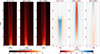 |
Fig. 3. Snapshots at three different time steps (t = 72 s, 240 s, and 996 s) after propagating kink waves are excited. (a1)–(a3) Normalised density (normalised with the code unit 109 cm−3) in the y = 0 plane. The dashed white lines indicate the unperturbed tube boundary (i.e. x = ±1 Mm). (b1)–(b3) vx at the x = 0 plane. Relevant animations are available online. |
The evolution of the flux tube is further illustrated with time-distance (TD) maps in Figure 4. The TD maps of density at three different heights all show sinusoidal transverse displacements, which is a typical characteristic of kink waves. The effect of density stratification and resonant absorption can be seen in panels b1–b3, which present TD maps of LOS velocity (i.e. vx at x = 0 plane). The velocity amplitude at the tube centre (inside the inhomogeneous boundary layer) represents the energy of driven bulk kink waves. It first increases from z = 0 Mm to 40 Mm and then decreases from 40 Mm to 80 Mm. The increase is due to the density decreasing with height, as a result of gravity. However, the resonant absorption is already in effect, which can be inferred from the formation of fine structures at the boundary layer. As indicated in, for example, Terradas et al. (2010), Pascoe et al. (2010), and Soler et al. (2011), the energy of kink waves transfers to azimuthal Alfvén modes in the inhomogeneous layer, leading to a coupling of kink mode and Alfvén mode. The effect of resonant absorption becomes more dominant as the height increases, because at every height, the transverse motions (in a coupling state of kink and Alfvén modes) act as a new wave source. Then the coupling state is inherited by waves at higher heights, and resonant absorption can develop based on this state (e.g. Pascoe et al. 2011, 2013; Hood et al. 2013; De Moortel & Howson 2022). In fact, if we constrain the driver to only one period, the kink wave in the tube centre will decay very quickly and soon there will be only torsional Alfvén waves at the tube boundary, as shown in Pascoe et al. (2010, 2012) and Pagano & De Moortel (2017). In contrast, in our case with a continuous driver and density stratification, the kink wave will not be quickly damped; instead, its amplitude can be amplified at lower heights due to the altitude variation in density. Nevertheless, resonant absorption dominates at higher heights, leading to a reduced amplitude at z = 80 Mm. We can further obtain the velocity amplitude at each height (z0) by fitting the time series of vx(0, 0, z0) (see below). The amplitude reaches its peak at z ∼ 45 Mm. Below that height, the stratification-induced amplitude increase is more dominant; while over that height, the resonant damping becomes more effective. It is consistent with the statement that the amplitude is simply a product of these two effects given in Soler et al. (2011).
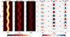 |
Fig. 4. TD maps at three different heights (z = 0 Mm, 40 Mm, and 80 Mm). (a1)–(a3) Normalised density at y = 0. The dashed white lines indicate the unperturbed tube boundary (i.e. x = ±1 Mm). (b1)–(b3) vx at x = 0. |
3.2. Development of small-scale structures and relevant heating
In contrast to kink waves, the azimuthal Alfvén waves generated by resonant absorption have a non-collective characteristic, which means that they can propagate at multiple magnetic surfaces each with a different Alfvén speed (e.g. Terradas et al. 2010; Soler & Terradas 2015). Thus, phase mixing can form at the boundary layer, manifested as a deformed wavefront (Heyvaerts & Priest 1983). The joint effect of resonant absorption and phase mixing leads to the small-scale structures appearing in the tube boundary in Figures 4b2 and b3.
To further illustrate these small-scale structures, we plot the cross-section profiles of density and temperature at z = 40 Mm and 80 Mm at t = 1140 s, as shown in Figure 5. We can see some finger-like density structures in Figures 5a1 and a2, suggesting the initiation of KHI due to velocity shearing related to phase mixing. However, from the relevant animations, the development of KHI seems to be suppressed to a limited level. In contrast, for standing kink waves, the KHI can fully develop after resonant absorption and phase mixing, eventually leading to the formation of a turbulent state (e.g. Terradas et al. 2008; Antolin et al. 2014, 2015, 2016; Okamoto et al. 2015; Howson et al. 2017; Karampelas et al. 2017, 2019; Guo et al. 2019, 2020, 2023b; Shi et al. 2021a,b). Specifically, the KHI vortices, which are a natural result for standing kink waves, cannot be generated in our simulation (for further discussion see Section 5.3).
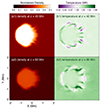 |
Fig. 5. Cross-section profiles of (a) density and (b) temperature at t = 1140 s. The upper and lower rows correspond to different heights (z = 40 Mm and 80 Mm). An animation is available online. |
As indicated in the previous studies (Pagano & De Moortel 2017; Pagano et al. 2018, 2020), although KHI-induced turbulent vortices and non-linear state may not exist, phase mixing can still lead to some energy dissipation and heating by generating smaller structures. In Figure 5b, we can see that the most significant temperature variations occur in the boundary layer, suggesting a direct association with resonant absorption and phase mixing here. However, there are both regions where temperature increases and decreases (compared to the initial uniform temperature of ∼1 MK), which could be interpreted as adiabatic heating (cooling) instead of real dissipation (see e.g. Karampelas et al. 2017; Guo et al. 2019).
We then calculated the surface averaged temperature at every height and every time step. During the calculation, we restricted the region to be −2 to 2 Mm in both the x and y directions. Moreover, the oscillating flux tube does not go beyond this sub-region. The results are depicted in Figure 6a. Considering that there might be some numerical issues near the lower boundary (z = 0 Mm), here we only focused on the part above 5 Mm. The temperature below 25 Mm decreases with time, while a temperature increase exists in parts above 25 Mm (also the main part of the flux tube). Furthermore, the amount of temperature change (ΔT) also increases with height (see also the solid blue line in Figure 6c). In Figure 6b, we plot time series of temperature averaged in the volume from z = 5 Mm to 100 Mm, which also shows a growing trend, rising by approximately 6000 K within 20 min.
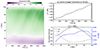 |
Fig. 6. Temperature changes in the simulation. (a) Temporal and height variations in the surface-averaged temperature. (b) Time series of the volume-averaged temperature within [−2, 2] Mm × [−2, 2] Mm × [5, 100] Mm. (c) The solid and dashed black lines depict the height dependence of normalised |


There may be two main factors that contribute to the increase in average temperature: viscous dissipation and Ohmic (resistivity) dissipation. We calculated the values of  and
and  by averaging them at each height over the time range from t = 0 to 1200 s, and plot them (after normalisation) as a function of height z in Figure 6c. They can be compared with the temperature change ΔT during the same time range. Roughly speaking, the heating effect appears to be more pronounced at the heights where the vorticity is relatively large and the current density is relatively low. Therefore, for propagating kink waves, viscous dissipation might be more efficient in converting wave energy into thermal energy. Furthermore, our numerical setup introduces a quite large numerical resistivity (see Section 2), but the spatial distributions of
  and ΔT barely show any correlation, which further suggests that resistivity dissipation may not be dominant. In comparison, heating induced by standing modes inside closed coronal loops exhibits a clear preference at lower heights (near footpoints) where resistivity dissipation is more significant, while viscosity dissipation dominates near the loop apex (see Van Doorsselaere et al. 2007; Antolin et al. 2014; Karampelas et al. 2017; Guo et al. 2019; Shi et al. 2021a,b). Further understanding of the contributions from these two dissipation mechanisms for propagating kink waves is important but beyond the scope of our current study.
3.3. Analysis of energy density
The analysis of volume averaged energy density can reveal valuable information of the system (e.g. Karampelas et al. 2019; Guo et al. 2019; Shi et al. 2021a,b). We estimated the energy density inside the same volume (V0) as that in Figure 6b, namely, [−2, 2] Mm × [−2, 2] Mm × [5, 100] Mm. Following Karampelas et al. (2019), the kinetic (K(t)), magnetic (M(t)), internal (I(t)), and gravitational (G(t)) energy density variations are given by:
 (7)
(7)
 (8)
(8)
 (9)
(9)
 (10)
(10)
where γ = 5/3 is the adiabatic index, and Φ denotes the gravitational potential. The total energy density variation is
 (11)
(11)
For comparison, we also performed a new run without the footpoint driver. The time series of energy density for both runs are shown in Figure 7a. During the no-driver run (indicated by dashed lines), the total energy experiences a decrease with time because the energy can be lost from the boundaries, especially from the upper boundary which is set as an extended outflow boundary with artificial velocity absorption (see Section 2 and Figure 2). However, this can be acceptable because plumes in the coronal hole are naturally associated with mass and energy loss caused by the solar wind (e.g. Poletto 2015; Morton et al. 2015; Tian et al. 2021).
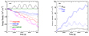 |
Fig. 7. Results of the energy analysis. (a) Time series for the magnetic (red), internal (blue), kinetic (black), gravitational (green), and total (magenta) energy density relative to t = 0. Solid and dashed lines represent simulation runs with and without a wave driver, respectively. (b) Time series of increased internal energy due to wave energy (ΔItotal, the solid black line), total input energy from the wave driver (Sinput, the solid blue line), and the ‘trapped’ portion of input energy (Stotal, the dashed blue line). |
For the run with a driver (marked by solid lines), we can see an increase in kinetic energy relative to the no-driver case, which is obviously due to the input of Poynting flux carried by the driver. However, the magnetic energy decreases faster than that of the no-driver case. This could be a result of increased lateral energy leakage through side boundaries after kink waves are excited (see e.g. Guo et al. 2019; Shi et al. 2021b). The internal energy has a slight increase compared to the no-driver case, suggesting that the propagating kink wave can indeed dissipate the kinetic energy and lead to an increase in the internal energy of the system.
In Figure 7b, we plot the input energy density Sinput(t) inside V0 with a solid blue line, which is estimated as
 (12)
(12)
where Ab denotes the area of the bottom boundary. However, not all of the input energy (Poynting flux) can remain inside the volume V0. As mentioned above, there is also energy flux escaping through the upper boundary. Thus, we also calculated how much energy can be ‘trapped’ inside V0, given by
 (13)
(13)
where A includes all six outer surfaces of V0. The evolution of Stotal(t) is depicted by the dashed blue line in Figure 7b, and it approximately saturates at around 2 × 10⁻⁵ J m−3. This trapped energy can partially convert to internal energy, manifesting as the internal energy increase ΔI (relative to the no-driver case, shown by the black line in Figure 7b).
4. Forward modelling with FoMo
It is of interest to investigate the observational properties of propagating kink waves in our simulation. Here we employed the FoMo code (Van Doorsselaere et al. 2016) to forward-model the numerical results. The Fe IX 17.1 nm line is utilised because it is a typical coronal line in studying propagating transverse waves (e.g. McIntosh et al. 2011; Thurgood et al. 2014; Morton et al. 2015; Weberg et al. 2018, 2020). For every snapshot (time step), we can obtain the synthesised spectra as a data cube with three dimensions: new x or y (depending on different LOSs), new z, and wavelength λ. Then we performed a single Gaussian fit to the line profiles at each pixel to obtain the 2D map of line intensity, Doppler velocity, and line width. In Figure 8, we plot TD maps for these parameters at z = 40 Mm.
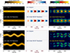 |
Fig. 8. TD maps of forward modelling results at z = 40 Mm. The upper and lower rows correspond to the LOS view and POS view (defined in Section 4), respectively. (a) TD maps of the Fe IX 17.1 nm line intensity with the original spatial resolution and a degraded resolution comparable to AIA. (b) and (c) TD maps of the Doppler velocity and line width with the original spatial resolution and a degraded resolution comparable to that of MUSE. Panels d–f: same but for the POS view. Panel d1: demonstrates how we obtained the wave parameters from the intensity TD maps. The tube centre positions are marked with black triangles, and the sinusoidal fitting results are depicted with a white curve. |
We chose two different LOS angles for the forward modelling. The first one is parallel to the x axis (shown in Figures 8a–c), with the dominant velocity perturbation along the LOS; and the second one is parallel to the y axis (shown in Figures 8d–e), with the dominant velocity perturbation perpendicular to LOS (or in the POS). Therefore, we name these two cases the LOS view and the POS view.
To directly compare FoMo results with observations, we also degraded the original spatial resolution with the method described in Chen et al. (2021). For the line intensity, the resolution was degraded to match SDO/AIA EUV imaging observations, which have a pixel size of 0.6″ (∼0.44 Mm) and a spatial resolution of 1.5″ (Lemen et al. 2012). Meanwhile, the Doppler velocity and line width can only be obtained by coronal EUV spectrometers. Although the Fe IX 17.1 nm line is not included in the coronal spectrometers currently at work, the Multi-slit Solar Explorer (MUSE; De Pontieu et al. 2020), a proposed mission scheduled for launch in 2027, will have the capability to acquire high-resolution 17.1 nm spectra. Hence, here we degraded the original maps of Doppler velocity and line width to the spatial resolution (0.4″) of MUSE. Finally, we extracted our simulation outputs every 12 s, matching the cadence achievable by both AIA and MUSE (Lemen et al. 2012; De Pontieu et al. 2020, 2022).
4.1. LOS view
We first focus on the results of the LOS view. As expected, we cannot see any transverse displacements from the original intensity TD maps (Figure 8a1). Interestingly, there are some variations in the tube width and intensity with time, which have been usually interpreted as longitudinal waves such as sausage waves before (e.g. Morton et al. 2012; Tian et al. 2016; see also the review by Li et al. 2020). However, these features are actually related to the cross-section deformation of the flux tube when it oscillates transversely (that is, moving forwards and backwards periodically for this view). For example, when the flux tube returns to its initial position, the velocity perturbation reaches the largest, causing the cross-section to stretch from a circle to an elliptical shape, with a slightly reduced span perpendicular to the velocity (see the online animation associated with Figure 5). It further leads to the change of integrated optically thin emissions. Similar scenarios can be found in Cooper et al. (2003) and Yuan & Van Doorsselaere (2016) for standing kink waves. Another potential explanation is associated with the first fluting mode generated by non-linearity (see Ruderman et al. 2010). After degrading to AIA resolution (Figure 8a2), the change of tube width cannot be captured, although some signatures of periodic intensity oscillation still remain, with a period that is approximately half of the wave period.
For standing kink waves in closed coronal loops, forward modelling reveals that some apparent strands along the loop can be created as an LOS effect of KHI, offering a potential approach to observing this instability in coronal loops (Antolin et al. 2014). Conversely, here we cannot produce such strand-like features, possibly due to the insufficient development of KHI for propagating modes as described in Section 3.2. However, the periodic brightening observed in the intensity TD maps, as shown in Figure 8a2, may provide a novel way to indirectly observe signatures of propagating kink waves when the velocity perturbation is in the LOS. The result also suggests that detecting such signals using AIA imaging data could be achievable, and it may be even easier with higher resolution observations from the Extreme Ultraviolet Imager (EUI; Rochus et al. 2020) on board the Solar Orbiter (Müller et al. 2020). Furthermore, we can easily distinguish such kink-wave-induced intensity variations from longitudinal waves (e.g. Meadowcroft et al. 2024) because their propagating speeds differ significantly; the former would be one or two orders of magnitude larger than the latter (Morton et al. 2015; Liu et al. 2015; Jess et al. 2016). As a result, it appears promising to detect such signatures with SDO/AIA or Solar Orbiter/EUI in the near future.
From the TD map of Doppler velocity shown in Figure 8b, we can clearly see the kink wave signals presenting as the alternately generating red and blue shifts, as well as the phase mixing in the boundary layer. Such a pattern can be also found in the case of standing waves (Antolin et al. 2017; Guo et al. 2019). Additionally, the boundary characteristics can be detected under the MUSE resolution, which suggests that MUSE will have the capability to directly detect the signals of resonant absorption and phase mixing of propagating kink waves. Furthermore, the fine structures at the tube boundary are also captured by the TD map of line widths from Figure 8c. Considering that the temperature across the flux tube is close to 1 MK, the thermal width can be estimated by  km s−1, where kb and mion are the Boltzmann constant and mass of the ion Fe IX, respectively. Hence, the pattern presented here reflects the temporal and spatial variation in the non-thermal broadening or non-thermal velocity (vnth), which can be naturally enhanced by generation of small-scale structures at the tube boundary.
Another interesting feature is that the line width fluctuates in the tube centre with about half the wave period (∼150 s). The largest line width (∼20 km s−1) gives a non-thermal velocity of  km s−1. This feature will be further discussed in the next subsection.
4.2. POS view
The forward modelling results of the POS view are relatively simple. The intensity, as shown in Figure 8d, oscillates transversely and sinusoidally over time, similar to previous observational studies with AIA (McIntosh et al. 2011; Thurgood et al. 2014; Morton et al. 2015; Weberg et al. 2018, 2020). Also, as expected, no apparent Doppler velocity signals can be seen in Figure 8e. However, in the realistic case, when there is an inclination angle between the LOS and the direction of this view, there will be observable Doppler signals (as a projection of main velocity perturbations). Such a case has been investigated in standing wave simulations such as Antolin et al. (2015, 2017) and Guo et al. (2019).
As for the line width shown in Figure 8f, the appearance of intensified non-thermal broadening is related to the formation of small-scale structures by phase mixing in the boundary layer. However, the development of these signals quickly saturates, suggesting that the phase-mixing-induced KHI will not fully develop into a turbulent state, consistent with the results presented in Section 3.2 and relevant animations of Figure 5. Moreover, the non-thermal broadening exhibits a periodic variation that is simultaneous with that in the tube centre of the LOS view, and thus provides an interpretation of the patterns shown in Figure 8c. Specifically, the variation in the tube centre can be regarded as the result of a superposition of the non-thermal broadening at both boundaries. Finally, the degraded TD map (panel f2) illustrates that MUSE might have sufficient spatial and temporal resolutions to capture these localised fine structures. However, the total line width (∼18.5 km s−1) is only slightly larger than the thermal width (∼17 km s−1), which appears likely to be covered by the instrumental broadening and noise, and thus may not be resolved in real observations.
Although the non-thermal velocities we obtained here appears to be too small to be detected for a single flux tube, we can expect that when there are multiple tubes in the LOS, the integration effect will generate a much larger vnth that is comparable to the results of spectral observation (∼20−50 km s−1; see e.g. Van Doorsselaere et al. 2008; Banerjee et al. 2009; Hahn et al. 2012; Bemporad & Abbo 2012; Hahn & Savin 2013; Morton et al. 2015; Zhu et al. 2021, 2024). Most previous studies tend to interpret observed non-thermal line broadening as a result of torsional Alfvén waves or Alfvén wave turbulence. However, our findings suggest that the LOS superposition of multiple flux tubes carrying kink waves can also generate the observed vnth, further supporting the conclusion in previous studies (McIntosh & De Pontieu 2012; Pant et al. 2019; Pant & Van Doorsselaere 2020; Fyfe et al. 2021).
4.3. Altitude variations in wave parameters
In imaging observations, there is a set of techniques widely used to estimate wave parameters including amplitude and period from intensity TD maps. Specifically, the first step is to determine the tube centre with a Gaussian fitting (e.g. Thurgood et al. 2014; Anfinogentov et al. 2015) or some empirical thresholds of intensity spatial gradient (e.g. Weberg et al. 2018, 2020). With the time series of tube centre positions (i.e. displacements), we can perform fitting with a sine function (e.g. Thurgood et al. 2014) or conduct Fourier transformation (e.g. Duckenfield et al. 2018; Weberg et al. 2018, 2020; Bate et al. 2022; Zhong et al. 2023a) to obtain the displacement amplitude ξ and period P. Subsequently, the velocity amplitude can be calculated as
 (14)
(14)
Here we adopted the similar analysis techniques described in Gao et al. (2022, 2024) with intensity TD maps at every height from 0 to 100 Mm to obtain the wave amplitude and period as a function of height (z). An example is shown in Figure 8d1 with the tube centre positions marked by black triangles and the fitted sinusoidal curve marked by the solid white line.
The altitude variation in these wave parameters is presented in Figure 9. The dashed lines in panel a are amplitudes acquired from the TD maps based on FoMo results, with the black (blue) one indicating the velocity (displacement) amplitude; while the solid line, as described in Section 3.1, is the velocity amplitude calculated with original simulation output data. All of them exhibit a similar trend with height, peaking at about 45 Mm. However, the difference between the solid and dashed black lines implies that the velocity amplitude obtained from imaging observations using Equation (14) may potentially underestimate the amplitude and, consequently, the associated energy flux. Another plausible explanation for this discrepancy could be some averaging and LOS integration effects, as we only used vx at the z axis to obtain the amplitude corresponding to the solid black line.
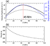 |
Fig. 9. Height variation in the wave parameters. (a) Height variation in the velocity (black) and displacement (blue) amplitude, with the dashed red line indicating the position where the amplitude reaches the maximum (z = 45 Mm). (b) Height variation in the wave period. The solid black line is extracted from the original simulation output data, and all other dashed lines in both panels are obtained with forward modelling results as described in Section 4.3. |
From Figure 9b, it appears that the period undergoes a slight but consistent decrease with height, ranging from 300 s at z = 0 Mm to 283 s at z = 100 Mm. This trend is likely attributed to errors stemming from the fitting method when there is a non-oscillatory stage in TD maps (as shown in Figure 8d). This stage exists because the wavefront requires time to propagate to a specific height. As the height increases, such a stage persists for a longer duration, resulting in an underestimation of the period. When extending the time series for fitting (e.g. to 1200 s), the period at all heights can return to a value very close to the driver period (300 s), which is expected. However, here we choose to present forward modelling results and conduct fitting for only a relatively short duration (approximately 2.5 oscillation cycles), because in observations it is rare to detect propagating kink wave events with more cycles (Weberg et al. 2018, 2020). Thus, Figure 9b provides valuable insights for future observational studies, indicating the importance of carefully removing the non-oscillatory part before extracting wave parameters, particularly the periods. Given that wave periods play an important role in coronal seismology (e.g. Nakariakov & Ofman 2001; Zhong et al. 2023b) and energy estimations (e.g. Bate et al. 2022; Petrova et al. 2023; Lim et al. 2023), a thorough investigation on how analysis techniques affect period measurement is desired in the future.
5. Discussion
5.1. Implications for coronal seismology of relative density profiles
For propagating kink waves, the velocity amplitude can be expressed as (e.g. Soler et al. 2011; Morton et al. 2012; Weberg et al. 2020)
 (15)
(15)
where C is a constant, and R(z) is the radius of the flux tube at the height of z, which is also nearly constant for our model. Another simplified parameter is the magnetic field B, which varies very little in the whole simulation domain (see Figure 1(c)). Thus, the kink speed ck(z) is proportional to  , and finally we have
 (16)
(16)
Such a relation is utilised by some observational studies to derive the relative density profile as a function of height in the corona, especially the open-field region (Morton et al. 2015; Weberg et al. 2020). Similar seismology methods have also been used in other structures such as spicules (Verth et al. 2011), jets (Morton et al. 2012), chromospheric mottles (Kuridze et al. 2013), and fibrils (Morton 2014). However, Equation (16) does not consider the variation in the amplitude due to the combined effects of resonant absorption and the stratification (see Section 3.1). Therefore, here we assessed the seismology method with the simulation data to further investigate the effect of resonant absorption.
In Figure 10a, we plot the relation between velocity amplitude (derived based on forward modelling result with Equation 14) and average density at the same height in the log-log scale. We only selected the data samples below 45 Mm, where vamp increases with height. There is no linear correlation with a slope of −1/4 between these two values (as marked by the dashed red line). Equation (16) can be further examined by calculating  (the slope in Figure 10a) as a function of height, which is shown in Figure 10b. The theoretical value without considering resonant damping should be −1/4. We can see that, aside from very low altitudes where resonant absorption may not be well developed (see also Figure 4b1), the calculated derivative values generally fall below the theoretical value of −1/4, with the deviation increasing at higher altitudes. Hence, if we still use Equation (16) to derive the relative density change, there will be an underestimation of density.
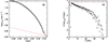 |
Fig. 10. Assessment of the seismology techniques used in previous studies (see Section 5.1). (a) Scatter plot between log⟨ρ⟩ and log vamp. The dashed red line indicates their theoretical relation with a slope of −1/4 based on Equation (16). (b) Derivative dlog vamp/dlog⟨ρ⟩ as a function of height (z). The theoretical value (−1/4) based on Equation (16) is also depicted with the dashed red line. We note that in panel a, the height decreases from left to right. |
Such a result is expected to be associated with the resonant damping rate, which can be quantified by the equilibrium parameter ξE:
 (17)
(17)
Then the damping length is:
 (18)
(18)
where λ is the wavelength. To validate our findings, we performed two additional runs: one with a larger ξE (achieved by reducing the density contrast ζ from 3 to 2) and another with a longer wavelength (achieved by increasing the period P from 300 s to 900 s) to investigate cases with larger LD. The results demonstrate that the deviation from −1/4 remains non-negligible for both runs. As a consequence, our simulation illustrates that, when conducting such seismological diagnostics, resonant absorption should be taken into account even if we observe an increasing amplitude with height as found in, for example, Morton et al. (2015) and Weberg et al. (2020). Specifically, the resonant damping could lead to an underestimation of the average density when applying Equation (16). Moreover, according to Equation (16), the density is proportional to the fourth power of the velocity amplitude, which can significantly amplify any error brought from vamp, further stressing the lack of robustness of this seismology method.
The conclusion drawn here may provide an additional explanation for the results in Weberg et al. (2020). They applied Equation (17) and observed vamp as a function of height to derive the relative density profile above the solar limb. In their Figure 7, a rapid decrease in the derived relative density between 5 and 10 Mm suggests the presence of an extended transition region up to this height. However, this is much larger than the classical transition region height of approximately 1−2 Mm (e.g. Avrett & Loeser 2008) above the solar surface. Weberg et al. (2020) interpreted the discrepancy as a potential result of dynamic fibrils and spicules reaching high in the corona (see e.g. De Pontieu et al. 2007; Pereira et al. 2012). However, if resonant absorption is considered, the discrepancy can be attributed to the underestimation of density when using Equation (16) in a quite straightforward way. Based on Figure 10a, when the velocity amplitude increases from 100.88 (∼7.6) km s−1 to 100.93 (∼8.5) km s−1, representing a 15% increase, the derived density can show a decreasing by approximately 60% if resonant damping is not considered. In contrast, if resonant damping is taken into account, the density only decreases by about 10%. Therefore, neglecting damping can exaggerate the density gradient, leading to an overestimation of the transition region height.
Further consideration should be given to the limitations of our current model, particularly regarding the disparities between our model and the actual solar atmosphere. Our current simulation does not include the cross-section area expansion and magnetic field weakening with height (see e.g. Soler et al. 2011; Ruderman et al. 2013, 2019; Lopin & Nagorny 2017; Guo et al. 2024) for simplification. However, the magnetic flux conservation gives that B(z)R(z)2 is approximately a constant for a flux tube. Thus, according to Equation (15) and  , the relation (16) remains valid regardless of any height variations of B(z) and R(z) as long as the magnetic flux is conserved. Nevertheless, the expansion of the flux tube and longitudinal inhomogeneity of the magnetic field may influence the wave behaviour and strength of resonant absorption (e.g. Fedun et al. 2011; Lopin & Nagorny 2017; Howson et al. 2019; Soler et al. 2019; Ruderman et al. 2019); hence it would be interesting to investigate wave properties in an expanding magnetic flux tube with 3D MHD simulations in the future (currently, such works are mostly analytical). Recently, Howson et al. (2019) developed a model for an expanding closed coronal flux tube, focusing on standing kink waves. However, in their model, the density remains uniform throughout the simulation domain. Thus, a more realistic MHD model, combining both density and magnetic field inhomogeneity, should be established and explored in future studies.
Another important seismological application of propagating kink waves is to diagnose the coronal Alfvén speed and magnetic field by measuring its phase speed (Morton et al. 2015; Long et al. 2017; Magyar & Van Doorsselaere 2018; Yang et al. 2020a,b; Baweja et al. 2024). Our model is suitable for assessing such seismology techniques, which will be the topic of a forthcoming paper.
5.2. Propagating kink waves and the energy balance in the coronal open-field region
As described in Section 3.2 and 3.3, propagating kink waves might have a potential contribution to the energy balance in coronal open-field regions, or coronal holes. According to the estimation in Withbroe & Noyes (1977), the solar wind flux dominates the energy loss in the coronal hole, much larger than that of thermal conduction and radiative cooling. In our simulation, this energy loss can be roughly reflected in the decrease in energy density shown in Figure 7a, particularly for the no-driver case (dashed lines). For the case with a kink wave driver (see Figure 7b), most input wave energy (Sinput) flows out from the upper boundary, while some energy (Stotal) can remain in the corona. The latter can be dissipated and partially transformed into internal energy, which may contribute to compensating the radiative loss and driving the solar wind.
There are two potential approaches to enhancing wave heating efficiency to balance the energy loss (apart from the solar wind flux) in the coronal hole. The first one is to input more energy at the lower boundary, which can be achieved by increasing the amplitude or frequency of the driver (e.g. Karampelas et al. 2019) and/or employing a broad-band driver instead of a mono-periodic one (e.g. Pascoe et al. 2015; Magyar et al. 2017; Magyar & Van Doorsselaere 2018; Pagano & De Moortel 2019; Pagano et al. 2020). However, further investigation requires a detailed parameter survey, which exceeds the scope of this study. The second approach is to augment the dissipation rate of wave energy into internal energy, which is associated with the development of KHI and turbulence, and will be discussed in the subsequent subsection.
5.3. KHI development of propagating waves
In our simulation, the efficiency of energy dissipation is constrained by the incomplete development of the KHI and relevant turbulence (see Section 3.2). This is one of the primary distinctions between propagating and standing modes. It has been known since the early 1980s that propagating Alfvén waves undergoing phase mixing are stable to KHI while standing waves are unstable (Heyvaerts & Priest 1983). As indicated by Zaqarashvili et al. (2015), for propagating (coupled) Alfvén waves induced via resonant absorption, the magnetic and velocity perturbations are out of phase. An external horizontal magnetic field parallel to the velocity shearing can increase the instability threshold and consequently stabilise the KHI (e.g. Bennett et al. 1999; Li et al. 2018). Consequently, when the velocity perturbation attains its peak, the magnetic field perturbation also reaches its maximum but in the opposite direction, thereby suppressing KHI. Conversely, for standing modes, the velocity amplitude peaks at the antinodes (e.g. the loop apex for fundamental oscillations of a closed coronal loop), while the magnetic perturbation there is zero (e.g. Zaqarashvili 2003; Guo et al. 2020). Hence, KHI can be easily induced, with its heating effect shown to sufficiently counterbalance radiative losses in closed coronal loops (Shi et al. 2021b).
In fact, most previous numerical studies on propagating kink waves, including ours, have not reported the (fully) development of KHI (Pascoe et al. 2010, 2011, 2012; Zaqarashvili et al. 2015; Pagano & De Moortel 2017; Howson et al. 2020). However, Pagano & De Moortel (2019) reported that KHI can be generated with propagating modes, with the flux tube significantly deformed. One possible explanation for this inconsistency is that they used the observed power spectrum (Tomczyk & McIntosh 2009) to set the wave driver, resulting in a driver that is in a nearly turbulent state. In such cases, the cylindrical symmetry of the flux tube might be broken, and instabilities could be more likely to occur (see Meringolo et al. 2024). Nonetheless, the findings of Pagano & De Moortel (2019) have put it under debate whether KHI can effectively form and develop for propagating kink waves (see also Section 4.2 in Morton et al. 2023).
In our simulation, the small-scale structures at the tube boundary (see Figure 5) may also be linked to uniturbulence (e.g. Magyar et al. 2017, 2019; Van Doorsselaere et al. 2020; Ismayilli et al. 2022), which describes the non-linear self-deformation of propagating kink waves, generating a cascade to smaller scales. Accepting this interpretation, it would be interesting to compare the energy cascade rate with theoretical predictions (e.g. Van Doorsselaere et al. 2020 but with modification to incorporate longitudinal stratification) in the future.
6. Conclusions
In this study, we conducted a 3D MHD simulation to investigate the behavior of propagating kink waves within a gravitationally stratified open magnetic flux tube. With both transverse and longitudinal density inhomogeneity incorporated, we can investigate their joint effect on these widely spread wave phenomena. Particularly, the consideration of gravitational stratification is missing in most previous numerical studies of the same type (Pascoe et al. 2010, 2011, 2012; Magyar et al. 2017; Magyar & Van Doorsselaere 2018; Pagano & De Moortel 2017, 2019; Pagano et al. 2020; Howson et al. 2020). Furthermore, we performed forward modelling with FoMo to synthesise observational properties. Such analyses have been extensively conducted for simulations of standing kink waves (e.g. Antolin et al. 2015, 2016, 2017; Guo et al. 2019; Shi et al. 2021a), but have rarely been applied to propagating modes within an individual open flux tube.
Our main findings can be summarised as follows:
1. Resonant absorption and gravitational stratification both influence the altitude variation in the wave amplitude. While stratification dominates at lower heights, resonant absorption becomes more prominent at higher altitudes. When diagnosing the relative density profile with Equation (16), resonant damping needs to be considered to avoid a possible underestimation, even in the regime where resonant damping is not dominant.
2. In contrast to standing kink modes, for propagating waves the KHI development appears to be suppressed after resonant absorption and phase mixing. Nonetheless, fine structures can still be formed in the tube boundary, leading to energy cascading on smaller scales and a slight temperature increase, especially at higher altitudes. A major portion of the input wave energy exits via the upper boundary, corresponding to the flux carried by the solar wind, while the remaining energy causes an internal energy increase, potentially contributing to balancing the radiative losses in coronal holes.
3. Forward modelling results highlight the promising potential of future high-resolution coronal imaging spectrometers (such as MUSE) in directly detecting signatures of resonant absorption and phase mixing. Moreover, transverse motions of the flux tube can produce periodical variations in TD maps of the intensity and the line width with half the wave period. Notably, the intensity could potentially be captured using current EUV imagers, such as SDO/AIA and Solar Orbiter/EUI.
Our future works will focus on enhancing the complexity of the model and the driver. This may involve extending the model to incorporate multiple flux tubes and/or the lower atmosphere. Additionally, the driver could be replaced with a broadband one to better mimic the actual transverse motions at the base of the corona. Within the coronal open-field region, other topics of interest include the connection with the solar wind (mass transport and acceleration), propagating intensity disturbances, and the influence of background flow on transverse waves. These topics are also worth investigating using our current model (or its modified versions).
Data availability
Movies associated to Figs. 3 and 5 are available at https://www.aanda.org
Acknowledgments
This work is supported by the National Natural Science Foundation of China grant 12425301 and the National Key R&D Program of China No. 2021YFA1600500. Y.G. acknowledges support from the China Scholarship Council under file No. 202206010018. M.G. acknowledges support from the National Natural Science Foundation of China (NSFC, 12203030). T.V.D. was supported by the European Research Council (ERC) under the European Union’s Horizon 2020 research and innovation programme (grant agreement No. 724326), the C1 grant TRACEspace of Internal Funds KU Leuven, and a Senior Research Project (G088021N) of the FWO Vlaanderen. Furthermore, TVD received financial support from the Flemish Government under the long-term structural Methusalem funding program, project SOUL: Stellar evolution in full glory, grant METH/24/012 at KU Leuven. The research that led to these results was subsidised by the Belgian Federal Science Policy Office through the contract B2/223/P1/CLOSE-UP. It is also part of the DynaSun project and has thus received funding under the Horizon Europe programme of the European Union under grant agreement (no. 101131534). Views and opinions expressed are however those of the author(s) only and do not necessarily reflect those of the European Union and therefore the European Union cannot be held responsible for them. K.K. acknowledges support by an FWO (Fonds voor Wetenschappelijk Onderzoek – Vlaanderen) postdoctoral fellowship (1273221N).
References
- Anfinogentov, S. A., Nakariakov, V. M., & Nisticò, G. 2015, A&A, 583, A136 [NASA ADS] [CrossRef] [EDP Sciences] [Google Scholar]
- Antolin, P., Yokoyama, T., & Van Doorsselaere, T. 2014, ApJ, 787, L22 [Google Scholar]
- Antolin, P., Okamoto, T. J., De Pontieu, B., et al. 2015, ApJ, 809, 72 [Google Scholar]
- Antolin, P., De Moortel, I., Van Doorsselaere, T., & Yokoyama, T. 2016, ApJ, 830, L22 [Google Scholar]
- Antolin, P., De Moortel, I., Van Doorsselaere, T., & Yokoyama, T. 2017, ApJ, 836, 219 [Google Scholar]
- Aschwanden, M. J., Fletcher, L., Schrijver, C. J., & Alexander, D. 1999, ApJ, 520, 880 [Google Scholar]
- Avrett, E. H., & Loeser, R. 2008, ApJS, 175, 229 [Google Scholar]
- Banerjee, D., Teriaca, L., Doyle, J. G., & Wilhelm, K. 1998, A&A, 339, 208 [Google Scholar]
- Banerjee, D., Pérez-Suárez, D., & Doyle, J. G. 2009, A&A, 501, L15 [NASA ADS] [CrossRef] [EDP Sciences] [Google Scholar]
- Banerjee, D., Krishna Prasad, S., Pant, V., et al. 2021, Space Sci. Rev., 217, 76 [NASA ADS] [CrossRef] [Google Scholar]
- Bate, W., Jess, D. B., Nakariakov, V. M., et al. 2022, ApJ, 930, 129 [NASA ADS] [CrossRef] [Google Scholar]
- Baweja, U., Pant, V., & Arregui, I. 2024, ApJ, 963, 69 [NASA ADS] [CrossRef] [Google Scholar]
- Bemporad, A., & Abbo, L. 2012, ApJ, 751, 110 [NASA ADS] [CrossRef] [Google Scholar]
- Bennett, K., Roberts, B., & Narain, U. 1999, Sol. Phys., 185, 41 [NASA ADS] [CrossRef] [Google Scholar]
- Chen, Y., Przybylski, D., Peter, H., et al. 2021, A&A, 656, L7 [NASA ADS] [CrossRef] [EDP Sciences] [Google Scholar]
- Cooper, F. C., Nakariakov, V. M., & Tsiklauri, D. 2003, A&A, 397, 765 [CrossRef] [EDP Sciences] [Google Scholar]
- De Moortel, I., & Howson, T. A. 2022, ApJ, 941, 85 [NASA ADS] [CrossRef] [Google Scholar]
- De Moortel, I., & Pascoe, D. J. 2012, ApJ, 746, 31 [Google Scholar]
- De Moortel, I., Pascoe, D. J., Wright, A. N., & Hood, A. W. 2016, Plasma Phys. Control. Fusion, 58, 014001 [Google Scholar]
- De Pontieu, B., Hansteen, V. H., Rouppe van der Voort, L., van Noort, M., & Carlsson, M. 2007, ApJ, 655, 624 [Google Scholar]
- De Pontieu, B., Martínez-Sykora, J., Testa, P., et al. 2020, ApJ, 888, 3 [NASA ADS] [CrossRef] [Google Scholar]
- De Pontieu, B., Testa, P., Martínez-Sykora, J., et al. 2022, ApJ, 926, 52 [NASA ADS] [CrossRef] [Google Scholar]
- Doschek, G. A., Mariska, J. T., Warren, H. P., et al. 2007, ApJ, 667, L109 [NASA ADS] [CrossRef] [Google Scholar]
- Duckenfield, T., Anfinogentov, S. A., Pascoe, D. J., & Nakariakov, V. M. 2018, ApJ, 854, L5 [Google Scholar]
- Fedun, V., Shelyag, S., & Erdélyi, R. 2011, ApJ, 727, 17 [NASA ADS] [CrossRef] [Google Scholar]
- Fyfe, L. E., Howson, T. A., De Moortel, I., Pant, V., & Van Doorsselaere, T. 2021, A&A, 656, A56 [NASA ADS] [CrossRef] [EDP Sciences] [Google Scholar]
- Gao, Y., Tian, H., Van Doorsselaere, T., & Chen, Y. 2022, ApJ, 930, 55 [NASA ADS] [CrossRef] [Google Scholar]
- Gao, Y., Guo, M., Van Doorsselaere, T., Tian, H., & Skirvin, S. J. 2023, ApJ, 955, 73 [NASA ADS] [CrossRef] [Google Scholar]
- Gao, Y., Hou, Z., Van Doorsselaere, T., & Guo, M. 2024, A&A, 681, L4 [NASA ADS] [CrossRef] [EDP Sciences] [Google Scholar]
- Goddard, C. R., Nisticò, G., Nakariakov, V. M., & Zimovets, I. V. 2016, A&A, 585, A137 [NASA ADS] [CrossRef] [EDP Sciences] [Google Scholar]
- Goossens, M., Terradas, J., Andries, J., Arregui, I., & Ballester, J. L. 2009, A&A, 503, 213 [NASA ADS] [CrossRef] [EDP Sciences] [Google Scholar]
- Goossens, M., Andries, J., Soler, R., et al. 2012, ApJ, 753, 111 [Google Scholar]
- Guo, M., Van Doorsselaere, T., Karampelas, K., et al. 2019, ApJ, 870, 55 [Google Scholar]
- Guo, M., Li, B., & Van Doorsselaere, T. 2020, ApJ, 904, 116 [Google Scholar]
- Guo, M., Duckenfield, T., Van Doorsselaere, T., et al. 2023a, ApJ, 949, L1 [NASA ADS] [CrossRef] [Google Scholar]
- Guo, M., Gao, Y., Van Doorsselaere, T., & Goossens, M. 2023b, A&A, 676, L7 [NASA ADS] [CrossRef] [EDP Sciences] [Google Scholar]
- Guo, M., Van Doorsselaere, T., Li, B., & Goossens, M. 2024, A&A, 687, A30 [NASA ADS] [CrossRef] [EDP Sciences] [Google Scholar]
- Hahn, M., & Savin, D. W. 2013, ApJ, 776, 78 [NASA ADS] [CrossRef] [Google Scholar]
- Hahn, M., Landi, E., & Savin, D. W. 2012, ApJ, 753, 36 [NASA ADS] [CrossRef] [Google Scholar]
- Heyvaerts, J., & Priest, E. R. 1983, A&A, 117, 220 [NASA ADS] [Google Scholar]
- Hood, A. W., Ruderman, M., Pascoe, D. J., et al. 2013, A&A, 551, A39 [NASA ADS] [CrossRef] [EDP Sciences] [Google Scholar]
- Howson, T. A., De Moortel, I., & Antolin, P. 2017, A&A, 602, A74 [NASA ADS] [CrossRef] [EDP Sciences] [Google Scholar]
- Howson, T. A., De Moortel, I., Antolin, P., Van Doorsselaere, T., & Wright, A. N. 2019, A&A, 631, A105 [NASA ADS] [CrossRef] [EDP Sciences] [Google Scholar]
- Howson, T. A., De Moortel, I., & Reid, J. 2020, A&A, 636, A40 [NASA ADS] [CrossRef] [EDP Sciences] [Google Scholar]
- Ismayilli, R., Van Doorsselaere, T., Goossens, M., & Magyar, N. 2022, Front. Astron. Space Sci., 8, 241 [NASA ADS] [CrossRef] [Google Scholar]
- Jess, D. B., Mathioudakis, M., Erdélyi, R., et al. 2009, Science, 323, 1582 [Google Scholar]
- Jess, D. B., Reznikova, V. E., Ryans, R. S. I., et al. 2016, Nat. Phys., 12, 179 [NASA ADS] [CrossRef] [Google Scholar]
- Karampelas, K., & Van Doorsselaere, T. 2024, A&A, 681, L6 [NASA ADS] [CrossRef] [EDP Sciences] [Google Scholar]
- Karampelas, K., Van Doorsselaere, T., & Antolin, P. 2017, A&A, 604, A130 [NASA ADS] [CrossRef] [EDP Sciences] [Google Scholar]
- Karampelas, K., Van Doorsselaere, T., & Guo, M. 2019, A&A, 623, A53 [NASA ADS] [CrossRef] [EDP Sciences] [Google Scholar]
- Kohutova, P., Verwichte, E., & Froment, C. 2020, A&A, 633, L6 [NASA ADS] [CrossRef] [EDP Sciences] [Google Scholar]
- Kuridze, D., Verth, G., Mathioudakis, M., et al. 2013, ApJ, 779, 82 [NASA ADS] [CrossRef] [Google Scholar]
- Lemen, J. R., Title, A. M., Akin, D. J., et al. 2012, Sol. Phys., 275, 17 [Google Scholar]
- Li, D., & Long, D. M. 2023, ApJ, 944, 8 [NASA ADS] [CrossRef] [Google Scholar]
- Li, X., Zhang, J., Yang, S., Hou, Y., & Erdélyi, R. 2018, Sci. Rep., 8, 8136 [CrossRef] [Google Scholar]
- Li, B., Antolin, P., Guo, M. Z., et al. 2020, Space Sci. Rev., 216, 136 [NASA ADS] [CrossRef] [Google Scholar]
- Li, D., Bai, X., Tian, H., et al. 2023, A&A, 675, A169 [NASA ADS] [CrossRef] [EDP Sciences] [Google Scholar]
- Lim, D., Van Doorsselaere, T., Berghmans, D., et al. 2023, ApJ, 952, L15 [NASA ADS] [CrossRef] [Google Scholar]
- Liu, J., McIntosh, S. W., De Moortel, I., & Wang, Y. 2015, ApJ, 806, 273 [NASA ADS] [CrossRef] [Google Scholar]
- Long, D. M., Valori, G., Pérez-Suárez, D., Morton, R. J., & Vásquez, A. M. 2017, A&A, 603, A101 [NASA ADS] [CrossRef] [EDP Sciences] [Google Scholar]
- Lopin, I., & Nagorny, I. 2017, AJ, 154, 141 [NASA ADS] [CrossRef] [Google Scholar]
- Magyar, N., & Van Doorsselaere, T. 2018, ApJ, 856, 144 [Google Scholar]
- Magyar, N., Van Doorsselaere, T., & Goossens, M. 2017, Sci. Rep., 7, 14820 [NASA ADS] [CrossRef] [Google Scholar]
- Magyar, N., Van Doorsselaere, T., & Goossens, M. 2019, ApJ, 882, 50 [Google Scholar]
- Mancuso, S., & Raymond, J. C. 2015, A&A, 573, A33 [NASA ADS] [CrossRef] [EDP Sciences] [Google Scholar]
- Mathioudakis, M., Jess, D. B., & Erdélyi, R. 2013, Space Sci. Rev., 175, 1 [Google Scholar]
- Matsumoto, T. 2018, MNRAS, 476, 3328 [NASA ADS] [CrossRef] [Google Scholar]
- McIntosh, S. W., & De Pontieu, B. 2012, ApJ, 761, 138 [NASA ADS] [CrossRef] [Google Scholar]
- McIntosh, S. W., de Pontieu, B., Carlsson, M., et al. 2011, Nature, 475, 477 [Google Scholar]
- Meadowcroft, R. L., Zhong, S., Kolotkov, D. Y., & Nakariakov, V. M. 2024, MNRAS, 527, 5302 [Google Scholar]
- Meringolo, C., Pucci, F., Nisticò, G., et al. 2024, A&A, 688, A12 [NASA ADS] [CrossRef] [EDP Sciences] [Google Scholar]
- Mignone, A., Bodo, G., Massaglia, S., et al. 2007, ApJS, 170, 228 [Google Scholar]
- Morton, R. J. 2014, A&A, 566, A90 [NASA ADS] [CrossRef] [EDP Sciences] [Google Scholar]
- Morton, R. J., Verth, G., McLaughlin, J. A., & Erdélyi, R. 2012, ApJ, 744, 5 [NASA ADS] [CrossRef] [Google Scholar]
- Morton, R. J., Tomczyk, S., & Pinto, R. 2015, Nat. Commun., 6, 7813 [Google Scholar]
- Morton, R. J., Weberg, M. J., & McLaughlin, J. A. 2019, Nat. Astron., 3, 223 [Google Scholar]
- Morton, R. J., Tiwari, A. K., Van Doorsselaere, T., & McLaughlin, J. A. 2021, ApJ, 923, 225 [NASA ADS] [CrossRef] [Google Scholar]
- Morton, R. J., Sharma, R., Tajfirouze, E., & Miriyala, H. 2023, Rev. Mod. Plasma Phys., 7, 17 [NASA ADS] [CrossRef] [Google Scholar]
- Müller, D., St. Cyr, O. C., Zouganelis, I., et al. 2020, A&A, 642, A1 [Google Scholar]
- Nakariakov, V. M., & Ofman, L. 2001, A&A, 372, L53 [NASA ADS] [CrossRef] [EDP Sciences] [Google Scholar]
- Nakariakov, V. M., Ofman, L., Deluca, E. E., Roberts, B., & Davila, J. M. 1999, Science, 285, 862 [Google Scholar]
- Nisticò, G., Nakariakov, V. M., & Verwichte, E. 2013, A&A, 552, A57 [NASA ADS] [CrossRef] [EDP Sciences] [Google Scholar]
- Okamoto, T. J., Antolin, P., De Pontieu, B., et al. 2015, ApJ, 809, 71 [NASA ADS] [CrossRef] [Google Scholar]
- Pagano, P., & De Moortel, I. 2017, A&A, 601, A107 [NASA ADS] [CrossRef] [EDP Sciences] [Google Scholar]
- Pagano, P., & De Moortel, I. 2019, A&A, 623, A37 [NASA ADS] [CrossRef] [EDP Sciences] [Google Scholar]
- Pagano, P., Pascoe, D. J., & De Moortel, I. 2018, A&A, 616, A125 [NASA ADS] [CrossRef] [EDP Sciences] [Google Scholar]
- Pagano, P., De Moortel, I., & Morton, R. J. 2020, A&A, 643, A73 [NASA ADS] [CrossRef] [EDP Sciences] [Google Scholar]
- Pant, V., & Van Doorsselaere, T. 2020, ApJ, 899, 1 [NASA ADS] [CrossRef] [Google Scholar]
- Pant, V., Magyar, N., Van Doorsselaere, T., & Morton, R. J. 2019, ApJ, 881, 95 [NASA ADS] [CrossRef] [Google Scholar]
- Pascoe, D. J., Wright, A. N., & De Moortel, I. 2010, ApJ, 711, 990 [Google Scholar]
- Pascoe, D. J., Wright, A. N., & De Moortel, I. 2011, ApJ, 731, 73 [Google Scholar]
- Pascoe, D. J., Hood, A. W., de Moortel, I., & Wright, A. N. 2012, A&A, 539, A37 [NASA ADS] [CrossRef] [EDP Sciences] [Google Scholar]
- Pascoe, D. J., Hood, A. W., De Moortel, I., & Wright, A. N. 2013, A&A, 551, A40 [NASA ADS] [CrossRef] [EDP Sciences] [Google Scholar]
- Pascoe, D. J., Wright, A. N., De Moortel, I., & Hood, A. W. 2015, A&A, 578, A99 [NASA ADS] [CrossRef] [EDP Sciences] [Google Scholar]
- Pascoe, D. J., De Moortel, I., Pagano, P., & Howson, T. A. 2022, MNRAS, 516, 2181 [NASA ADS] [CrossRef] [Google Scholar]
- Pelouze, G., Van Doorsselaere, T., Karampelas, K., Riedl, J. M., & Duckenfield, T. 2023, A&A, 672, A105 [NASA ADS] [CrossRef] [EDP Sciences] [Google Scholar]
- Pereira, T. M. D., De Pontieu, B., & Carlsson, M. 2012, ApJ, 759, 18 [Google Scholar]
- Pesnell, W. D., Thompson, B. J., & Chamberlin, P. C. 2012, Sol. Phys., 275, 3 [Google Scholar]
- Petrova, E., Magyar, N., Van Doorsselaere, T., & Berghmans, D. 2023, ApJ, 946, 36 [CrossRef] [Google Scholar]
- Petrova, E., Van Doorsselaere, T., Berghmans, D., et al. 2024, A&A, 687, A13 [NASA ADS] [CrossRef] [EDP Sciences] [Google Scholar]
- Poletto, G. 2015, Liv. Rev. Sol. Phys., 12, 7 [NASA ADS] [CrossRef] [Google Scholar]
- Rochus, P., Auchère, F., Berghmans, D., et al. 2020, A&A, 642, A8 [NASA ADS] [CrossRef] [EDP Sciences] [Google Scholar]
- Ruderman, M. S., Goossens, M., & Andries, J. 2010, Phys. Plasmas, 17, 082108 [Google Scholar]
- Ruderman, M. S., Pelinovsky, E., Petrukhin, N. S., & Talipova, T. 2013, Sol. Phys., 286, 417 [NASA ADS] [CrossRef] [Google Scholar]
- Ruderman, M. S., Shukhobodskaya, D., & Shukhobodskiy, A. A. 2019, Front. Astron. Space Sci., 6, 10 [Google Scholar]
- Sen, S., & Pant, V. 2021, ApJ, 923, 178 [NASA ADS] [CrossRef] [Google Scholar]
- Shi, M., Van Doorsselaere, T., Antolin, P., & Li, B. 2021a, ApJ, 922, 60 [NASA ADS] [CrossRef] [Google Scholar]
- Shi, M., Van Doorsselaere, T., Guo, M., et al. 2021b, ApJ, 908, 233 [Google Scholar]
- Skirvin, S. J., Gao, Y., & Van Doorsselaere, T. 2023, ApJ, 949, 38 [NASA ADS] [CrossRef] [Google Scholar]
- Soler, R., & Terradas, J. 2015, ApJ, 803, 43 [Google Scholar]
- Soler, R., Terradas, J., Verth, G., & Goossens, M. 2011, ApJ, 736, 10 [NASA ADS] [CrossRef] [Google Scholar]
- Soler, R., Terradas, J., Oliver, R., & Ballester, J. L. 2019, ApJ, 871, 3 [Google Scholar]
- Terradas, J., Arregui, I., Oliver, R., et al. 2008, ApJ, 679, 1611 [NASA ADS] [CrossRef] [Google Scholar]
- Terradas, J., Goossens, M., & Verth, G. 2010, A&A, 524, A23 [NASA ADS] [CrossRef] [EDP Sciences] [Google Scholar]
- Threlfall, J., De Moortel, I., McIntosh, S. W., & Bethge, C. 2013, A&A, 556, A124 [NASA ADS] [CrossRef] [EDP Sciences] [Google Scholar]
- Thurgood, J. O., Morton, R. J., & McLaughlin, J. A. 2014, ApJ, 790, L2 [Google Scholar]
- Tian, H., McIntosh, S. W., & De Pontieu, B. 2011, ApJ, 727, L37 [NASA ADS] [CrossRef] [Google Scholar]
- Tian, H., McIntosh, S. W., Wang, T., et al. 2012, ApJ, 759, 144 [Google Scholar]
- Tian, H., DeLuca, E. E., Cranmer, S. R., et al. 2014, Science, 346, 1255711 [Google Scholar]
- Tian, H., Young, P. R., Reeves, K. K., et al. 2016, ApJ, 823, L16 [Google Scholar]
- Tian, H., Harra, L., Baker, D., Brooks, D. H., & Xia, L. 2021, Sol. Phys., 296, 47 [NASA ADS] [CrossRef] [Google Scholar]
- Tiwari, A. K., Morton, R. J., & McLaughlin, J. A. 2021, ApJ, 919, 74 [NASA ADS] [CrossRef] [Google Scholar]
- Tomczyk, S., & McIntosh, S. W. 2009, ApJ, 697, 1384 [Google Scholar]
- Tomczyk, S., McIntosh, S. W., Keil, S. L., et al. 2007, Science, 317, 1192 [Google Scholar]
- Tomczyk, S., Card, G. L., Darnell, T., et al. 2008, Sol. Phys., 247, 411 [Google Scholar]
- van Ballegooijen, A. A., Asgari-Targhi, M., & Berger, M. A. 2014, ApJ, 787, 87 [NASA ADS] [CrossRef] [Google Scholar]
- Van Doorsselaere, T., Andries, J., & Poedts, S. 2007, A&A, 471, 311 [NASA ADS] [CrossRef] [EDP Sciences] [Google Scholar]
- Van Doorsselaere, T., Nakariakov, V. M., & Verwichte, E. 2008, ApJ, 676, L73 [Google Scholar]
- Van Doorsselaere, T., Antolin, P., Yuan, D., Reznikova, V., & Magyar, N. 2016, Front. Astron. Space Sci., 3, 4 [Google Scholar]
- Van Doorsselaere, T., Li, B., Goossens, M., Hnat, B., & Magyar, N. 2020, ApJ, 899, 100 [NASA ADS] [CrossRef] [Google Scholar]
- Verth, G., Terradas, J., & Goossens, M. 2010, ApJ, 718, L102 [NASA ADS] [CrossRef] [Google Scholar]
- Verth, G., Goossens, M., & He, J. S. 2011, ApJ, 733, L15 [NASA ADS] [CrossRef] [Google Scholar]
- Verwichte, E., Van Doorsselaere, T., White, R. S., & Antolin, P. 2013, A&A, 552, A138 [NASA ADS] [CrossRef] [EDP Sciences] [Google Scholar]
- Weberg, M. J., Morton, R. J., & McLaughlin, J. A. 2018, ApJ, 852, 57 [Google Scholar]
- Weberg, M. J., Morton, R. J., & McLaughlin, J. A. 2020, ApJ, 894, 79 [NASA ADS] [CrossRef] [Google Scholar]
- Withbroe, G. L., & Noyes, R. W. 1977, ARA&A, 15, 363 [Google Scholar]
- Yang, Z., Tian, H., Tomczyk, S., et al. 2020a, Sci. China E: Technol. Sci., 63, 2357 [CrossRef] [Google Scholar]
- Yang, Z., Bethge, C., Tian, H., et al. 2020b, Science, 369, 694 [Google Scholar]
- Yuan, D., & Van Doorsselaere, T. 2016, ApJS, 223, 23 [Google Scholar]
- Zaqarashvili, T. V. 2003, A&A, 399, L15 [CrossRef] [EDP Sciences] [Google Scholar]
- Zaqarashvili, T. V., Zhelyazkov, I., & Ofman, L. 2015, ApJ, 813, 123 [Google Scholar]
- Zhong, S., Nakariakov, V. M., Kolotkov, D. Y., et al. 2023a, Nat. Commun., 14, 5298 [NASA ADS] [CrossRef] [Google Scholar]
- Zhong, S., Nakariakov, V. M., Miao, Y., Fu, L., & Yuan, D. 2023b, Sci. Rep., 13, 12963 [NASA ADS] [CrossRef] [Google Scholar]
- Zhu, Y., Szente, J., & Landi, E. 2021, ApJ, 913, 74 [NASA ADS] [CrossRef] [Google Scholar]
- Zhu, Y., Szente, J., & Landi, E. 2023, ApJ, 948, 90 [NASA ADS] [CrossRef] [Google Scholar]
- Zhu, Y., Habbal, S. R., Ding, A., et al. 2024, ApJ, 966, 122 [NASA ADS] [CrossRef] [Google Scholar]
All Figures
|
Fig. 1. Illustration of the model setup. (a) Density distribution at the y = 0 plane after relaxation. (b) and (c) Horizontal profiles of the density and magnetic field along the x axis at three different heights (indicated by different line styles). (d) Vertical profile of the density, demonstrating gravitational stratification, with solid and dashed lines indicating density within and outside the flux tube, respectively. The black and red lines in panels b–d represent states before and after relaxation, respectively. We note that the magnetic field in the initial state (before relaxation) is uniform along the z axis, and hence there is only one black line in panel c. |
| In the text | |
|
Fig. 2. Dependence of the velocity absorption factor, α, on height (z, horizontal axis) and time (indicated by different lines). Green and yellow shading distinguishes the regions below and above 100 Mm. The latter can be regarded as an extended upper boundary, and we only analysed and discuss the results below 100 Mm (green shading). |
| In the text | |
|
Fig. 3. Snapshots at three different time steps (t = 72 s, 240 s, and 996 s) after propagating kink waves are excited. (a1)–(a3) Normalised density (normalised with the code unit 109 cm−3) in the y = 0 plane. The dashed white lines indicate the unperturbed tube boundary (i.e. x = ±1 Mm). (b1)–(b3) vx at the x = 0 plane. Relevant animations are available online. |
| In the text | |
|
Fig. 4. TD maps at three different heights (z = 0 Mm, 40 Mm, and 80 Mm). (a1)–(a3) Normalised density at y = 0. The dashed white lines indicate the unperturbed tube boundary (i.e. x = ±1 Mm). (b1)–(b3) vx at x = 0. |
| In the text | |
|
Fig. 5. Cross-section profiles of (a) density and (b) temperature at t = 1140 s. The upper and lower rows correspond to different heights (z = 40 Mm and 80 Mm). An animation is available online. |
| In the text | |
|
Fig. 6. Temperature changes in the simulation. (a) Temporal and height variations in the surface-averaged temperature. (b) Time series of the volume-averaged temperature within [−2, 2] Mm × [−2, 2] Mm × [5, 100] Mm. (c) The solid and dashed black lines depict the height dependence of normalised |
| In the text | |
|
Fig. 7. Results of the energy analysis. (a) Time series for the magnetic (red), internal (blue), kinetic (black), gravitational (green), and total (magenta) energy density relative to t = 0. Solid and dashed lines represent simulation runs with and without a wave driver, respectively. (b) Time series of increased internal energy due to wave energy (ΔItotal, the solid black line), total input energy from the wave driver (Sinput, the solid blue line), and the ‘trapped’ portion of input energy (Stotal, the dashed blue line). |
| In the text | |
|
Fig. 8. TD maps of forward modelling results at z = 40 Mm. The upper and lower rows correspond to the LOS view and POS view (defined in Section 4), respectively. (a) TD maps of the Fe IX 17.1 nm line intensity with the original spatial resolution and a degraded resolution comparable to AIA. (b) and (c) TD maps of the Doppler velocity and line width with the original spatial resolution and a degraded resolution comparable to that of MUSE. Panels d–f: same but for the POS view. Panel d1: demonstrates how we obtained the wave parameters from the intensity TD maps. The tube centre positions are marked with black triangles, and the sinusoidal fitting results are depicted with a white curve. |
| In the text | |
|
Fig. 9. Height variation in the wave parameters. (a) Height variation in the velocity (black) and displacement (blue) amplitude, with the dashed red line indicating the position where the amplitude reaches the maximum (z = 45 Mm). (b) Height variation in the wave period. The solid black line is extracted from the original simulation output data, and all other dashed lines in both panels are obtained with forward modelling results as described in Section 4.3. |
| In the text | |
|
Fig. 10. Assessment of the seismology techniques used in previous studies (see Section 5.1). (a) Scatter plot between log⟨ρ⟩ and log vamp. The dashed red line indicates their theoretical relation with a slope of −1/4 based on Equation (16). (b) Derivative dlog vamp/dlog⟨ρ⟩ as a function of height (z). The theoretical value (−1/4) based on Equation (16) is also depicted with the dashed red line. We note that in panel a, the height decreases from left to right. |
| In the text | |
Current usage metrics show cumulative count of Article Views (full-text article views including HTML views, PDF and ePub downloads, according to the available data) and Abstracts Views on Vision4Press platform.
Data correspond to usage on the plateform after 2015. The current usage metrics is available 48-96 hours after online publication and is updated daily on week days.
Initial download of the metrics may take a while.