| Issue |
A&A
Volume 689, September 2024
|
|
|---|---|---|
| Article Number | A156 | |
| Number of page(s) | 16 | |
| Section | The Sun and the Heliosphere | |
| DOI | https://doi.org/10.1051/0004-6361/202450070 | |
| Published online | 09 September 2024 | |
Transition region response to quiet-Sun Ellerman bombs
1
Institute of Theoretical Astrophysics, University of Oslo, PO Box 1029, Blindern, 0315 Oslo, Norway
2
Rosseland Centre for Solar Physics, University of Oslo, PO Box 1029, Blindern, 0315 Oslo, Norway
3
Indian Institute of Astrophysics, II Block, Koramangala, Bengaluru 560 034, India
Received:
22
March
2024
Accepted:
11
June
2024
Abstract
Context. Quiet-Sun Ellerman bombs (QSEBs) are key indicators of small-scale photospheric magnetic reconnection events. Recent high-resolution observations have shown that they are ubiquitous and that large numbers of QSEBs can be found in the quiet Sun.
Aims. We aim to understand the impact of QSEBs on the upper solar atmosphere by analyzing their spatial and temporal relationship with the UV brightenings observed in transition region diagnostics.
Methods. We analyzed high-resolution Hβ observations from the Swedish 1-m Solar Telescope and utilized k-means clustering to detect 1423 QSEBs in a 51 min time series. We used coordinated and co-aligned observations from the Interface Region Imaging Spectrograph (IRIS) to search for corresponding signatures in the 1400 Å slit-jaw image (SJI) channel and in the Si IV 1394 Å and Mg II 2798.8 Å triplet spectral lines. We identified UV brightenings from SJI 1400 using a threshold of 5σ above the median background.
Results. We focused on 453 long-lived QSEBs (> 1 min) and found 67 cases of UV brightenings from SJI 1400 occurring near the QSEBs, both temporally and spatially. Temporal analysis of these events indicates that QSEBs start before UV brightenings in 57% of cases, while UV brightenings lead in 36% of instances. The majority of the UV brightenings occur within 1000 km of the QSEBs in the direction of the solar limb. We also identify 21 QSEBs covered by the IRIS slit, four of which show emissions in the Si IV 1394 Å and/or Mg II 2798.8 Å triplet lines, at distances within 500 km of the QSEBs in the limb direction.
Conclusions. We conclude that a small fraction (15%) of the long-lived QSEBs contribute to the localized heating observable in transition region diagnostics, indicating they play a minimal role in the global heating of the upper solar atmosphere.
Key words: Sun: activity / Sun: atmosphere / Sun: magnetic fields / Sun: transition region
Corresponding author; This email address is being protected from spambots. You need JavaScript enabled to view it. .
© The Authors 2024
 Open Access article, published by EDP Sciences, under the terms of the Creative Commons Attribution License (https://creativecommons.org/licenses/by/4.0), which permits unrestricted use, distribution, and reproduction in any medium, provided the original work is properly cited.
This article is published in open access under the Subscribe to Open model. This email address is being protected from spambots. You need JavaScript enabled to view it. to support open access publication.
1. Introduction
Ellerman bombs (EBs) were first identified by Ellerman (1917), who termed them “solar hydrogen bombs.” They occur at sites with opposite magnetic polarities in close proximity, where magnetic reconnection takes place. EBs are prominent in the hydrogen Balmer-α (Hα) line as small-scale, short-lived enhancements of the spectral line wings and are often observed in solar active regions with magnetic flux emergence (see, e.g., Georgoulis et al. 2002; Pariat et al. 2004; Fang et al. 2006; Pariat et al. 2007; Matsumoto et al. 2008; Watanabe et al. 2008; Libbrecht et al. 2017). When viewed toward the limb at high spatial and temporal resolution, they appear as bright, rapidly flickering flame-like structures that are rooted in the photosphere (Watanabe et al. 2011; Rutten et al. 2013; Nelson et al. 2015). The spectral profile of their Hα line has a characteristic moustache shape (Severny 1964), with enhanced emission in the wings and a dark absorption line core. Vissers et al. (2013) found that EBs also show signatures in the UV 1600 and 1700 Å passbands observed by Solar Dynamics Observatory (SDO; Pesnell et al. 2012).
Rouppe van der Voort et al. (2016) discovered quiet-Sun Ellerman-like brightenings, or quiet-Sun Ellerman bombs (QSEBs), through Hα observations made with the Swedish 1-m Solar Telescope (SST; Scharmer et al. 2003) in regions far from active regions. Joshi et al. (2020) find that the QSEBs are much more prevalent than earlier estimates suggested using, for the first time, Hβ observations from SST. They find that around half a million QSEBs can be present on the Sun at a given time. Rouppe van der Voort et al. (2024) increased this estimate to 750 000 QSEBs. They employed the shorter-wavelength Hε line, which provides higher spatial resolution and a larger contrast, leading to an increase in the number of QSEB detections. This large number of detections raises questions about their possible impact on energy transfer in the lower solar atmosphere.
Ultraviolet (UV) bursts can be identified as intense brightenings in Interface Region Imaging Spectrograph (IRIS) observations of the Si IV spectral lines (Peter et al. 2014). They are typically less than 2″ in size, and their duration can range from seconds to more than an hour (Young et al. 2018). These phenomena occur in regions of opposite magnetic polarities, analogous to the conditions of EBs. The spectral signatures of Si IV are often characterized by broadened emission lines with weak absorption blends from neutral or singly ionized species, leading to the inference that the hot UV bursts are located below the colder chromospheric canopy of fibrils (Peter et al. 2014). Vissers et al. (2015) provide examples of co-spatial and co-temporal EBs and UV bursts using IRIS spectra, particularly in the Mg II triplet and Si IV lines; they find that the tops of EBs might reach transition-region-like temperatures, that is to say, significantly higher temperatures than previously thought. Tian et al. (2016) found ten UV bursts either directly or potentially linked to EBs, all of which were characterized by notable Hα wing brightening without any signature in the line core. The examination of EBs by Libbrecht et al. (2017), with a specific focus on neutral helium triplet lines, further expanded our understanding of their properties. They find that EBs must reach high temperatures, in the range 2 × 10⁴–105 K.
Hansteen et al. (2019) employed a 3D radiative magnetohydrodynamic Bifrost model of a network region with a strong magnetic field injected 2.5 Mm beneath the solar surface. Their study reveals that EBs and UV bursts can occur either simultaneously or with some time difference along extended current sheets and are interconnected within the same reconnection system, with EBs occurring from the low photosphere up to 1200 km, and UV bursts from 700 km to 3 Mm above the photosphere. They also note potential offsets in EB and UV burst occurrences, influenced by the orientation of the current sheet and the viewing angle. Ortiz et al. (2020) and Chen et al. (2019) provide the observational perspective of the above scenario and explore the temporal and spatial interplay between EBs and their counterparts in the chromosphere and transition region. Until now, the only reported transition region response to a QSEB was by Nelson et al. (2017), based on coordinated Hα observations from the SST and IRIS. In this work, we further explore the connection between QSEBs and higher atmospheric diagnostics. In particular, this study explores the spatial and temporal relationship between QSEBs and associated brightenings in the IRIS Si IV observations to understand the dynamics between these events.
2. Observations
A quiet-Sun region close to the northern limb of the Sun was observed on 22 June 2021 by the CRisp Imaging SpectroPolarimeter (CRISP) and The CHROmospheric Imaging Spectrometer (CHROMIS; Scharmer et al. 2008) at the SST (Scharmer et al. 2003). The observing angle μ was 0.48 and the heliocentric coordinates were (x, y) = (4″, 827″). The observation started at 08:17:52 UT and ended at 09:08:32 UT, for a temporal duration of 51 min. CHROMIS was used to obtain the Hβ spectral line at 4861 Å across 27 line positions spanning ±2.1 Å around the line core. Within the inner wings at ±1.0 Å the sampling was done in 0.1 Å increments, with intervals becoming more spaced out in the outer wings to avoid blends. The CHROMIS observations have a temporal cadence of 7 s, pixel scale of 0 038 and cover an area of 66″ × 42″. CRISP ran a program sampling the Fe I 6173 Å, and Ca II 8542 Å spectral lines at a cadence of 19 s. Ca II 8542 Å was sampled in 4 line positions without polarimetry. Observations of the Fe I 6173 Å spectral line with polarimetry covered 13 line positions, spanning from ±0.16 Å in 0.04 Å intervals, extending to ±0.24 Å and ±0.32 Å along with the continuum located +0.68 Å away from the line core. In each line position, eight exposures were captured for each of the four polarization states, which, when considering the continuous cycling through four different states of the liquid crystal modulators, resulted in a total of 32 exposures per line position. The final CHROMIS and CRISP datasets used for the analysis are obtained through the SSTRED reduction pipeline (de la Cruz Rodríguez et al. 2015; Löfdahl et al. 2021). High-data quality were obtained with the aid of the SST adaptive optics system (Scharmer et al. 2024) and multi-object multi-frame blind deconvolution (MOMFBD; Van Noort et al. 2005) image restoration. For generating maps of the line-of-sight magnetic field strength (BLOS), Milne-Eddington inversions were performed on the Fe I 6173 Å observations using an inversion code by de la Cruz Rodríguez (2019). To determine the noise level for the line-of-sight magnetic field, BLOS, we selected a small area away from strong magnetic field concentrations. The noise level was then defined as the standard deviation within this selected region: 6.4 G. The lower-resolution CRISP data were aligned to the higher-resolution CHROMIS data by performing cross-correlation on the wideband channels. The lower cadence CRISP Fe I magnetograms were matched to the 7 s cadence CHROMIS data with nearest neighbor interpolation.
The quiet-Sun region was also co-observed with IRIS (De Pontieu et al. 2014). IRIS was running a “Large dense 4-step raster” program (OBS-ID 3633109417) and observed a bigger field of view (FOV) compared to the SST observation. The spectrograph slit covered an area of 1″ × 119″ by building up a raster of 4 slit positions with 0 35 separation. The raster cadence was 36 s with a step cadence of 9 s and each slit position has an exposure time of 8 s. The IRIS slit-jaw images (SJIs) cover a FOV of 120″ × 119″ and were taken with a cadence of 18 s for the 2796 Å channel (covering the chromospheric Mg II k line core) and 1400 Å channel (covering the two Si IV transition region lines). The IRIS data were spatially binned and have a pixel size of 0
 33. The SJIs were first rotated to match the orientation of the SST images. We then used the SJI 2796 Å for alignment of IRIS data to SST datasets by blowing up the IRIS data to CHROMIS pixel scale and performed cross-correlation between the wing positions of aligned Ca II 8542 Å and the SJI 2796 Å. The aligned IRIS data were then cropped to match the FOV of the CHROMIS data. The error in the co-alignment of these datasets is at least 1 IRIS pixel or better than that. Rouppe van der Voort et al. (2020) discuss the possible factors that can induce errors in the alignment.
In addition to a detailed analysis of the 22 June 2021 data, we also performed some analysis of a similar dataset from 25 July 2021. This is a 40 min time sequence of a quiet-Sun region at μ = 0.57. Both CRISP, CHROMIS, and IRIS were running the same observing programs. The seeing quality was similar to the June data. This July dataset was used to verify some of the results, such as the number of QSEB and UV brightening detections and spatial offsets between them. Furthermore, the IRIS raster spectra were explored for the possible presence of a strong UV burst-like event.
3. Method of analysis
3.1. Detection of QSEBs
We implemented the k-means clustering algorithm on our Hβ data, first employed by Joshi et al. (2020) for automatic detection of QSEBs. k-means clustering is a machine learning technique that groups a dataset into a predefined number of k clusters. During the initialization phase, we opted for the k-means++ method (Arthur & Vassilvitskii 2007). More details on this are available in Joshi & Rouppe van der Voort (2022). After establishing initial clusters, each cluster is represented by its cluster center (representative profile), which is the mean of all data points assigned to that cluster.
Before performing the clustering of the full dataset, we created a subset of data to make a cluster model that was used to predict the clustering of all 426 time steps. We started the clustering with 100 clusters on this subset as in (Joshi & Rouppe van der Voort 2022), but this did not give any clusters with clear QSEB-type spectral profiles. Therefore, we created a subset from selected profiles from the ten best-seeing scans and from frames 0–180. Hence, we opted for creating a biased training dataset, making sure that it contains spectral profiles representing QSEBs in the following way. From the chosen subset, we picked data points that show intensity enhancements in a few wavelength positions in the wings of the Hβ line profile – comprising EBs and magnetic bright points. We also keep some profiles corresponding to the bright centers of granules. In this way, we have a dataset that for 81% consists of profiles with strong wing intensity, and 19% of other types of profiles. We used this dataset to train the k-means model and found that we could reduce the number of clusters to 64. We identified 27 clusters that have representative profiles (RPs) similar to QSEBs. From the selected RPs, we predict the QSEBs from the full time series. After this we track the QSEBs temporally, utilizing the Trackpy library of Python, which initially identifies the central coordinate of each QSEB and assigns them a unique event ID number. Trackpy links the events over time and records information about each event ID – including the coordinates of the centers at each timestep, and the start and end times of the events. Following this, we implement connected component analysis from OpenCV. For each event ID, a region encompassing 26 pixels in space and time (as used by Joshi & Rouppe van der Voort 2022) is analyzed to identify all pixels that are occupied by the QSEB. This analysis checks for any pixel connected to the central coordinate pixel, whether horizontally, vertically, or diagonally. Through this temporal and spatial tracking of QSEBs, each QSEB has an event ID number, and information about the duration and region occupied by it at each timestep, which can be used for further in-depth analysis.
To refine our event selection, we set specific criteria: events that occur just for one timestep and have a maximum area of less than 5 pixels are excluded. So, any large event occurring for one timestep or any small event occurring for more than one timestep are considered as QSEBs. Furthermore, two events are considered as a single event if they are separated by a temporal gap of no more than 35 s, which is equal to 5 timesteps. This criterion was decided by checking how the mask from k-means detection evolves for a few QSEBs. Five timesteps allows for some variations in the k-means detection. Sometimes a QSEB can go through a phase when the spectral profiles do not pass the thresholds of the detection method. This can be due to for example seeing variations. By considering 5 timesteps we are linking the same QSEB in time, and it is not too long that we connect different events in time. Through this process, we have identified a total of 1423 QSEB events. We focused on the longer-lived QSEBs, of the 1423 events, that have duration exceeding 8 timesteps (≈1 min), resulting in a total of 453 such events. This is done because of the higher cadence of Hβ data and lower cadence of SJI data, giving enough SJI frames to check the evolution of UV brightening with the QSEB.
3.2. Detection of UV brightenings
The SJI 1400 images are full with short-lived and compact brightenings, most of them originate from acoustic waves and are related to the chromospheric bright grains observed in the Ca II H and K lines (Carlsson & Stein 1997). The signal in these grains in SJI 1400 comes mostly from the continuum rather than the Si IV lines (Martínez-Sykora et al. 2015). We are interested in investigating the connection between QSEBs and the brightest SJI 1400 events that are not related to acoustic waves. Following the approach of Young et al. (2018), who argued against a universal threshold for event identification in favor of dataset-specific criteria, we employed a threshold of 5σ above the median background to identify significant Si IV emissions in SJI 1400, henceforth referred to as “UV brightenings.” We found that a value of 5σ was most effective in identifying brightenings related to QSEBs. The threshold of 5σ is a conservative criterion to consider only the strongest events and avoid any ambiguous connections between the QSEBs and UV brightenings. It is possible that there could be more UV brightenings associated with the QSEBs by keeping a lower threshold, but these would not be the strongest events. We track and label these UV brightenings in a similar way as we did for the QSEBs. This approach resulted in the detection of 1978 such events. From the tracked QSEBs and UV brightening events, we identify those instances where UV brightenings are in immediate proximity to the 453 long-lived QSEBs, confined to a 4″ × 4″ area around the long-lived QSEB, and occur within 35 s of the start or end of the long-lived QSEB. After applying the above conditions, 199 of the 453 QSEBs have a nearby UV brightening. Out of the 1978 5σ UV brightenings, 272 are associated with the 199 QSEBs.
While most of the SJI 1400 signal in the chromospheric bright grains comes from the continuum, Martínez-Sykora et al. (2015) found that sometimes grains have shock signatures in the Si IV lines. To eliminate these short-lived shock-related grains, we employed a Fourier filter on the SJI 1400 dataset, adopting a 5 km s−1 cutoff as utilized by Gošić et al. (2018) in their examination of quiet-Sun atmosphere heating through internetwork magnetic field cancellations. Due to the presence of noise in the SJI data, the Fourier filtering creates artifacts around sharp peaks from cosmic ray hits to the detector. These artifacts influence the intensity threshold for determining the UV brightenings. Hence, instead of using the filtered SJI data, we check for those 272 UV brightening events to see if there is a considerable change in the intensity of the tracked events in the original data and in the filtered data and remove those events. This reduces the number of UV brightenings to 233, with 159 QSEBs associated with them. By applying the above criteria, we significantly reduced the risk of chance alignment of a shock with a QSEB. Also, by considering QSEBs with durations of more than 1 min we only focus on the strongest events, for which we can clearly see the evolution of the UV brightenings with the QSEB. We also removed many events for which the connection between QSEB and UV brightening was unclear. These are mentioned in the following paragraph. The removed QSEBs and UV brightenings could also be related, but we only focus on clear associations between these events for analysis.
In the analysis of the 159 QSEB – 233 UV brightening events, we identified instances where the association between QSEBs and UV brightenings was ambiguous, as some of the UV brightenings could not be associated with just the QSEB. For example, QSEBs amidst dense concentrations of magnetic bright points and large extended areas with Si IV emission. Other examples are isolated events where QSEB profiles are within an area with magnetic bright point profiles, and QSEBs adjacent to spicules not originating at the site of the QSEB. All these cases also have UV brightenings near them, which makes it difficult to associate them unambiguously with QSEBs. These observations led us to exclude such events, focusing on pairs where the UV brightening could be directly linked with the QSEB. We note here that we included events where the spicules originate very close to the QSEBs. This resulted in a total of 67 QSEB-UV brightening event pairs, which we use to study their spatial and temporal relationship.
Additionally, we focused on instances where the IRIS slit was positioned directly over QSEBs, finding 21 occurrences of this scenario. For these cases, we analyzed the emission characteristics in the Si IV 1394 Å and Mg II 2798.8 Å triplet spectral lines. Our analysis led to the identification of 4 QSEBs that exhibited notable enhancements in the Si IV 1394 Å and/or Mg II 2798.8 Å triplet lines.
4. Results
4.1. Temporal and spatial analysis of QSEBs and associated UV brightenings
From the 67 tracked QSEBs and UV brightening pairs, we present 5 events in Fig. 1, which shows the full FOV with zoomed-in boxes of the QSEBs and their associated 5σ brightenings. It is clear from the zoomed-in boxes that the UV brightenings usually occur at some spatial offsets from the QSEB in the direction toward the limb. Another example of a QSEB – UV brightening pair is shown in Fig. 2, which shows the temporal evolution of these events. The UV brightening occurs almost at the same spatial location as the QSEB. The blue cross denoting the center of QSEB lies at the boundary of the UV brightening in many instances, with the UV brightening occurring more in the direction of the solar limb. Even though the UV brightening is detected as a 5σ event 28 s after the QSEB begins, the same region in SJI is already bright when the QSEB starts. This suggests that there could be more UV brightenings associated with QSEBs by setting a lower threshold on the SJI 1400 images.
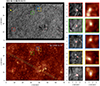 |
Fig. 1. Examples of QSEBs in the Hβ wing and their associated UV brightenings in the aligned SJI 1400. The QSEBs are outlined with red contours in the top-left panel. The 5σ brightenings are marked with yellow contours in the SJI 1400 panel (bottom left). The colored boxes in the left panels are shown at a higher magnification in the right columns, which display both the QSEBs and the UV brightenings. The zoomed-in boxes of SJI 1400 also show the red contours of the QSEBs near the UV brightenings. The yellow diagonal lines over the SJI mark the area that is covered by the IRIS spectrograph raster. The direction of the solar limb is shown by the yellow arrow in the Hβ wing image. |
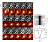 |
Fig. 2. Temporal evolution of a QSEB and associated UV brightening. The dark blue plus symbol marks the position of the QSEB in the Hβ −0.6 Å wing and a yellow plus symbol marks its position in SJI 1400. Black contours in SJI 1400 denote the UV brightening. The λt diagram to the right in panel (b) shows the spectral evolution at the pixel location marked with a plus in the Hβ wing. The light gray profile is an averaged reference profile. The vertical blue markers in panels b) and c) denote the Hβ line wing position for which the QSEB is shown in a). An animation of this figure, which shows the evolution of the QSEB with the UV brightening along with the Hβ spectral profile, is available online. |
The QSEB ends after 57 s, but the UV brightening continues for another 57 s. We looked for more such combined QSEB and UV brightening occurrences to gain a better understanding of their temporal and spatial dynamics. Within our dataset, we find a total of 67 QSEB – UV brightening event pairs. Among these, 59 QSEBs and 59 UV brightenings are uniquely identified, and we note instances where a single UV brightening is associated with multiple QSEBs, typically two to three, suggesting connectivity between them. Additionally, we observed that sometimes a UV brightening initiates before a QSEB begins, and another UV brightening starts later, close to the QSEB, with some temporal overlap with the QSEB.
Figure 3 presents a detailed visualization of the temporal relationship between QSEBs and UV brightenings. The timeline of each of the 67 events is normalized to the duration of each QSEB-UV brightening pair, allowing for a direct comparison across all events. From the 67 paired events, 53 coincide temporally to some extent, while the remaining 14, although not overlapping, happen within a span of 35 s of each other’s total duration. The possible scenarios of QSEB and UV brightening pairs occurrence are: (i) the QSEB and UV brightening start simultaneously, with the UV brightening ending first (e.g., events 1 and 2), (ii) the QSEB and UV brightening begin at different times but end at the same time (e.g., events 5 and 29), (iii) the QSEB occurs first with some temporal overlap with the UV brightening (e.g., events 33 and 34), (iv) the UV brightening occurs first, with some temporal overlap with the QSEB (e.g., events 28 and 32), (v) either the QSEB or the UV brightening persists for the entire observed period while the other occurs for some part of the duration (e.g., events 56 and 61), and (vi) either the QSEB or the UV brightening occurs first, but the other happens with some delay, with no temporal overlap (e.g., events 43 and 45). The example shown in Fig. 2 is event number 15. The QSEB started first, and the UV brightening started shortly after 20% of the 114 s combined duration. The QSEB ended at about the middle of the combined duration while the UV brightening reached peak intensity at about 70% of the combined duration.
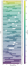 |
Fig. 3. Temporal evolution of the 67 QSEBs and UV brightening pairs. The events are shown in order of increasing duration. The combined duration of each event pair is given in seconds to the right of each bar. The duration of each QSEB and UV brightening is normalized to a common bar length. For each case, the lighter region of the bar denotes the time when the QSEB occurs, and the region marked with diagonal lines denotes the time when the UV brightening occurs. The darker part of the bar is the time when the QSEB and UV brightening occur together. The time of peak intensity of the QSEB is marked with a green dot, and the time of peak intensity of the UV brightening is marked with a red dot. |
Figure 4 illustrates the spatial distribution of the QSEBs and their corresponding UV brightenings superimposed on a map of the extreme values of BLOS within the full FOV. These events tend to cluster in areas where the magnetic field is notably stronger. The map showing these extreme BLOS values is also included in the top panel of the figure. The bottom panel shows some QSEBs marked by green circles. These are the events that occur multiple times during the full time series. From the uniquely identified 59 QSEBs, we observed that 24 repeatedly occurred at nine locations shown by the green circles. The events in Fig. 2 with red, green and blue boxes are three of those sites where both QSEBs and their associated UV brightenings occurred more than once during the entire time series.
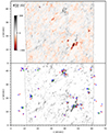 |
Fig. 4. Spatial distribution of the QSEBs, UV brightenings, and their magnetic environment. The top panel shows the extremum of BLOS at each pixel for the full 51 min duration of the time series. The bottom panel shows the QSEBs (red), and the UV brightenings (blue). The green circles represent the QSEBs that have multiple occurrences during the entire duration. In the background, dark gray areas indicates regions with |

The example presented in Fig. 2 demonstrates that a UV brightening can take place very close to the QSEB. The analysis of the 53 co-temporal pairs reveals a broad range of spatial offsets between QSEBs and UV brightenings. Figure 5 offers a statistical overview of these spatial offsets. It is important to note that the distances are measured in IRIS pixel units (1 pixel = 0 33), with each histogram bar corresponding to the angular size of an SST pixel equal to 0
 038. Panel a depicts the distances between the centroids of UV brightenings and QSEBs at each coinciding timestep. The majority (71%) of UV brightenings are situated 2–4 IRIS pixels away from QSEBs. A smaller portion (16%) of events are also found within 4–6 IRIS pixels, while others (13%) are located closer, within a 2-pixel distance. Likewise, panel b illustrates the separation between UV brightening boundaries and QSEBs, which depicts a slight reduction of the offset ranges. Since the boundaries of the UV brightenings are much closer to the QSEBs, we see that the bulk of events (73%) have boundaries 1–3 pixels away. Several are positioned extremely close (14%), within 1 pixel, while a few events (13%) are observed 3–5 pixels from the QSEB.
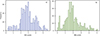 |
Fig. 5. Histograms of the distance from the QSEB centroid to the UV brightenings. Panel (a) shows the distance to the centroid of the UV brightenings, while panel (b) shows the distance to the nearest boundary of the UV brightenings. The size of each bin corresponds to the angular size of 1 SST pixel (0 |


Figure 6 gives a visual representation of how the UV brightenings occur in the surroundings of their QSEBs. The scatter plots vividly map out the spatial distribution of UV brightenings relative to their QSEB counterparts, as if each QSEB were placed at the center of the coordinate system. Panel a presents all co-temporal timesteps for each of the 53 QSEB-UV brightening pairs, utilizing markers with unique combinations of symbols and colors to denote the relative position of the centroids of UV brightenings with respect to their corresponding QSEBs. The numerous markers for each event highlight every instance where the QSEB-UV brightening pair occurs together. We find that markers for individual events are tightly clustered and show minor fluctuations in both distance and orientation relative to the QSEBs over the duration that the QSEB – UV brightening events occur together. Approximately 76% of UV brightenings are located within ±65deg with respect to the QSEB, with a small spatial offset toward the direction of the solar limb. In a similar way, panel b presents the distribution of the boundaries of the UV brightenings with the QSEB at the center. Here, the markers used for individual events are the same as for those events in panel a. This allows for a clear comparison of the spatial offsets of the centroids and boundaries for each event. The event boundaries are significantly nearer to the QSEB, and have a similar spread across the figure as in panel a. Similarly, the majority of the events (75%) reside within the ±65deg vicinity of the QSEB.
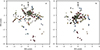 |
Fig. 6. Spatial distribution of the 53 co-temporal UV brightenings around the QSEBs. Each QSEB is put at the center of the figure denoted by the shaded red circle. For each UV brightening, the colored markers are shown for all the overlapping instances of occurrence, and at distances and angles calculated with their respective QSEBs. Panel a distributes the UV brightenings based on the distance of their centroids from the QSEBs. Panel b distributes the UV brightenings based on the distance of their nearest boundaries from the QSEBs. The direction of the nearest solar limb is toward the north. Here, the x and y axis have units in IRIS pixels (1 pixel = 0 |

4.2. Analysis of QSEBs captured by the IRIS slit
In our dataset, we identified 21 QSEBs that are covered by the IRIS slit. For each of these events, we examined the presence of emissions in the Mg II triplet 2798.8 Å and Si IV 1394 Å spectral lines. Among these, the spectral profiles of 17 events either exhibited noise or showed enhancements that were not significantly distinguishable. However, we present four cases where notable emissions were observed in the core of the Si IV line and/or in the wings of the two Mg II triplet lines, which are situated between the Mg II k and Mg II h lines (Pereira et al. 2015). For these cases, the intensity of the spectral lines shown in the figures has been divided by the exposure time of 8 s, and are therefore in units of DN s−1.
4.2.1. Spectral analysis of QSEB-1
Panel a of Fig. 7 presents an example of a QSEB, shown in the blue wing of the Hβ line. Moving to panel e, the spectra show the characteristic EB profile with clear enhancement in the wings of the Hβ line, which lasted for 65 s. Panel b displays the line-of-sight magnetic field, BLOS, and shows that the QSEB originates in a region of negative magnetic polarity near similar magnitude positive polarity. In the SJI 1400 observations, we found that the slit was often precisely covering the QSEB location. For the timesteps when the slit did not sample the region where the QSEB occurred, 5σ events were also observed in SJI 1400 throughout the QSEB’s lifetime. This can be clearly seen in the accompanying movie.
 |
Fig. 7. Snapshot of images and spectra of QSEB – 1 at the instance of maximum Si IV 1394 Å emission. The QSEB is located at y = 126 (in IRIS pixels) and at t = 08 : 40 : 24 UT. The top row shows the QSEB in Hβ −0.6 Å, the BLOS map with contours at 3σ above the noise level, and SJI 2796 and 1400. The 5σ contours are shown in yellow in SJI 1400. The lower row shows the normalized intensity in Hβ at the point of crossing of the cyan lines in the above Hβ −0.6 Å image. The spectral profiles of Mg II k 2796.39 Å, the Mg II triplet 2798.8 Å, and Si IV 1394 Å are shown for the region covered by the slit at y = 127, which is at a spatial offset of one pixel from the location of QSEB and are in units of DN s−1. An animation of this figure is available online. |
Figure 7 presents a snapshot that captures the peak emission in the Si IV 1394 Å line. This is also the strongest Si IV emission observed for co-temporal, co-spatial QSEB, and UV brightenings detected in this work. The Si IV profile exhibits a redshift and has a Doppler shift of +18 km s−1. We note that panels f, g, and h show the spectral profiles for Mg II k, Mg II triplet, and Si IV, which are offset by 1 IRIS pixel toward the limb from the QSEB location.
The Mg II k profile in panel f is broader than the quiet reference profile but does not stand out as different from profiles in the vicinity. This is also valid for the Mg II triplet lines in panel g, which does not show any enhancement. However, the associated movie displays occasional intensity enhancements in the wings of the Mg II triplet line throughout the event’s duration. Additionally, the Si IV 1394 Å line shows increased emission and subtle broadening at several timesteps concurrent with the QSEB. These panels further highlight regions shaded in pink for the Mg II triplet and green for the Si IV line, which we use for generating a time sequence of spectroheliograms for these wavelength ranges in Figs. 8 and 9. These show the evolution of the integrated line intensities over time and space (x-axis) against the pixels along the slit (y-axis).
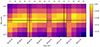 |
Fig. 8. Time series of Mg II triplet spectroheliograms for QSEB – 1. The log of the normalized integrated line intensity for Mg II triplet 2798.8 Å line shown by the pink shaded region in Fig. 7g is displayed in the spectroheliograms. A sequence of four rasters is shown, each raster consists of four slit positions marked with r1–r4 at the top. The vertical dotted lines mark the end of each raster. The black vertical lines denote the start and end time of the QSEB and the black horizontal line denotes the location of the QSEB-1. |
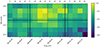 |
Fig. 9. Time series of Si IV spectroheliograms for QSEB – 1. The log of the normalized integrated line intensity for Si IV 1394 Å line shown by the green shaded region in Fig. 7h. Like in Fig 8, the vertical dashed lines mark the end of each of the rasters and the black vertical lines denote the start and end time of the QSEB. The black horizontal line denotes the location of the QSEB-1. |
Specifically, in Fig. 8, the spectroheliogram reveals that the intensity increase in the Mg II triplet starts approximately half a minute before the start of the QSEB and at the location where the QSEB occurs and continues while the QSEB is in progress. The location and duration of the QSEB in Hβ is marked with solid lines. Figure 9 presents the spectroheliogram for Si IV 1394 Å, highlighting that the peak emission for Si IV occurs between 08:40:24 and 08:41:08 UT shown by the yellow pixels. This also corresponds to the time when the QSEB exhibits its maximum wing enhancement of Hβ line and happens in a region 1–2 IRIS pixels above the location where the QSEB occurs.
4.2.2. Spectral analysis of QSEB-2
Figure 10 illustrates another QSEB, visible in the Hβ blue wing. Panel e shows the spectral profile, which exhibits notable, although moderate, wing enhancement in the Hβ line, observable for about 3 min. Panel b shows the (BLOS) magnetic field, with the QSEB emerging in a negative polarity patch amidst nearby positive polarity regions. In SJI 1400, we see that throughout the event’s duration, the slit frequently captures the QSEB directly. However, when the QSEB occurs outside the immediate area of the slit, the nearby areas are marked by distinct high-intensity events that exceed the 5σ level in several timesteps. Figure 10 presents the images and spectral profiles corresponding to the moment when the emission of the Si IV 1394 Å line reaches its maximum intensity for this case. Here, the profiles are also from the location at a spatial offset of 1 IRIS pixel toward the limb. The Si IV profile is slightly blue-shifted with a Doppler shift of −7.3 km s−1. The Mg II k line and the Mg II triplet profiles exhibit no notable enhancements for this particular snapshot. But, the accompanying movie highlights a consistent enhancement in the Mg II triplet wings, persisting throughout the entire duration of the event, for example, at time 08:53:08 UT. Moreover, the Si IV 1394 Å line shows both increased emission and a subtle broadening in sync with the QSEB. The Mg II triplet spectroheliogram (Fig. 11) shows that the most intense (brightest yellow) part is located just one pixel above the QSEB site. This intensity begins to surge at the start of the QSEB, reaching its maximum between 08:53:30 and 08:54:06 UT. Interestingly, the strongest emission in the wings of the Hβ line of the QSEB coincides with this phase of increased intensity, occurring around 08:53:43 UT. Figure 12 for Si IV 1394 Å highlights the peak emission timing, from 08:53:12 to 08:54:07 UT, occurring one pixel above the QSEB’s location and aligning with the Hβ line’s maximum wing enhancement. Another subtle increase in the intensity of Hβ wings occurs toward the end of the QSEB, for instance, at 08:54:48 UT, which is also accompanied by an enhancement in the Si IV 1394 Å line intensity. This is visible as light green patches at an offset of 1 IRIS pixel in the spectroheliogram of Fig. 12, just before the QSEB ends.
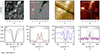 |
Fig. 10. Snapshot of images and spectra of QSEB – 2 at the instance of maximum Si IV 1394 Å emission, with the same format as Fig. 7. The QSEB is located at y = 124 (in IRIS pixels) at t = 08 : 53 : 29 UT. The spectral profiles of Mg II k 2796.39 Å, Mg II triplet 2798.8 Å, and Si IV 1394 Å are shown for the region covered by the slit at y = 125, which is at a spatial offset of one pixel from the location of QSEB and are in units of DN s−1. An animation of this figure is available online. |
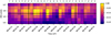 |
Fig. 11. Time series of spectroheliograms for QSEB – 2 of the log of the normalized integrated line intensity for Mg II triplet line. The black vertical lines denote the start and end time of the QSEB and the black horizontal line denotes the location of the QSEB-2. |
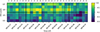 |
Fig. 12. Time series of spectroheliograms for QSEB – 2 of the log of the normalized integrated line intensity for Si IV 1394 Å line. The black vertical lines denote the start and end time of the QSEB and the black horizontal line denotes the location of the QSEB-2. |
4.2.3. Spectral analysis of QSEB-3
The third example, shown in Fig. 13, illustrates the scenario where the UV brightening occurs before the QSEB. From the movie associated with this figure, it can be seen that the UV brightening initiates before the QSEB, starting at 08:21:55 UT, with its intensity peaking at 08:23:11 UT. The Si IV 1394 Å line has predominantly a redshifted profile during the entire time. Figure 13 shows the images and spectral profiles for the instance with maximum emission and significant broadening of the Si IV 1394 Å line, which has a Doppler shift of +54.2 km s−1 at this time. As can be seen from panels e and g, the Hβ and Mg II triplet profiles are almost similar to the average quiet-Sun profile shown by the dashed lines. Interestingly, during periods of strong Si IV enhancement, there is a small reduction in the intensity of the Mg IIk2r spectral feature, falling below the quiet-Sun average. The Mg II k core is redshifted as shown in Fig. 13, and there is a decrease in intensity of k2r, suggesting that the line core opacity is shifted to that of k2r. This creates an opacity window that increases the intensity of k2v of Mg II k indicating downflows in the region. Similar opacity shifts and opacity window effects have been discussed by Bose et al. (2019) for the formation of Mg II k spectral line in type-II spicules.
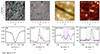 |
Fig. 13. Snapshot of images and spectra of QSEB – 3 at the instance of maximum Si IV 1394 Å emission, with the same format as Fig. 7. The QSEB occurs later in time and is located at y = 191 (in IRIS pixels) at t = 08 : 24 : 21 UT. The spectral profiles of Mg II k 2796.39 Å, Mg II triplet 2798.8 Å, and Si IV 1394 Å are shown for the region covered by the slit at the site of QSEB and are in units of DN s−1. An animation of this figure is available online. |
The QSEB itself begins at 08:25:24 UT and concludes at 08:26:49 UT, with its peak wing enhancement occurring at 08:26:06 UT. Figure 14 corresponds to the snapshot when the QSEB has maximum Hβ wing emission. Following this peak, although the wing enhancement diminishes, the line core brightening becomes more pronounced. After examining the Hβ line core, it was noted that the onset of brightening occurred at 08:26:06 UT (time of the snapshot in Fig. 14) and progressed toward the top of the QSEB in the direction of the solar limb. At the same time, there was a subtle emission in the wings of the Mg II triplet line too, which is shown at the location of the QSEB. The Si IV emission continues until approximately 08:26:21 UT. The QSEB emerges over a region of positive magnetic polarity as seen in panel (b) of Fig. 14, closely surrounded by areas of negative polarity. At instances when the slit drifts from the immediate area, the region’s activity remains detectable through 5σ brightening events, although only in a couple of timesteps. Panel (h) in both figures shows a wider green-shaded region compared to the previous cases due to the broadening and redshift of the Si IV profiles. The spectroheliogram for this shaded region is shown in Fig. 15, which distinctly illustrates that the Si IV emission occurs at the same location as the QSEB. The emission initiates prior to the QSEB and continues with less intensity during the QSEB.
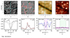 |
Fig. 14. Snapshot of images and spectra of QSEB – 3 at the instance of maximum emission in the wings of the Hβ line, with the same format as Fig. 7. The QSEB is located at y = 191 (in IRIS pixels) at t = 08 : 26 : 06 UT. Panel e) shows the normalized intensity of the Hβ line. The spectral profiles of Mg II k 2796.39 Å, Mg II triplet 2798.8 Å and Si IV 1394 Å are shown for the region covered by the slit at the site of QSEB and are in units of DN s−1. |
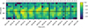 |
Fig. 15. Time series of spectroheliograms for QSEB - 3. The log of the normalized integrated line intensity for Si IV 1394 Å line is considered over a wider green shaded region shown in Figs. 13 and 14. |
4.2.4. QSEB with the strongest emission in the Mg II triplet lines
The QSEB shown in Fig. 16 occurs for about 2 min 23 s and is characterized initially by significant enhancements in the Hβ line wings. At 14 s from the start of the QSEB, the enhancement of the wings reaches its maximum, subsequently followed by the most pronounced emission in the Mg II triplet lines wings. This occurs around 28 s into the event and is located at an offset of 1 IRIS pixel (at y = 184). The QSEB occurs at y = 183 in IRIS pixels. An increase in the wings’ intensity of the Mg II triplet lines is also noted at 64 s at the same location as before, coinciding with an intensity enhancement in the wings of the Hβ line at 65 s. The QSEB initiates with a notable brightening of the Hβ line core, which, after 86 s, intensifies further, accompanied by a decrease in wing intensity. A snapshot of the QSEB at a later phase at 108 s in Fig. 16 shows the instance with maximum line core brightening of the Hβ line. It is also observed that the line core brightening occurs more at the top of the QSEB, which is toward the solar limb, compared to the profiles at 14 s and 65 s. Additionally, emissions from the Mg II triplet lines wings are observed at 92 s and 129 s, although less prominent than the peak emission at 28 s. This emission has also shifted by 1 IRIS pixel toward the limb, compared to the spectral profiles at 28 s and 64 s.
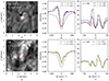 |
Fig. 16. Example of a QSEB with significant emission in the Mg II triplet lines. Panel (a) QSEB during the early phase at 14 s, which has significant wing enhancement of the Hβ spectral line. Normalized Hβ intensity is shown in panel (b) at two instances of 14 s and 65 s. Panel (c) shows the Mg II triplet profile during this early phase for two timesteps at 28 s and 64 s from y = 184 in IRIS pixels. Panel (d) shows the QSEB at 108 s during the end phase when the line core brightening of Hβ is more prominent. Spectral profiles for Hβ are shown in panel (e) for timesteps at 108 s and 129 s and for a location that is located at the top of the QSEB, which is slightly closer to the limb. Similar to panel (c), the Mg II triplet profiles are shown in panel (f) for two timesteps during the end phase of the QSEB, located at y = 185 in IRIS pixels and have units as DN s−1. |
5. Discussion
We have studied the transition region response to QSEBs, with a particular emphasis on the spatial and temporal interplay between QSEBs and UV brightenings. This was achieved by detecting QSEBs in Hβ and UV brightenings from IRIS imaging and spectrograph data. We conclude that QSEBs can show significant emissions in SJI 1400 and also in the Si IV 1394 Å and Mg II 2798.8 Å triplet spectral lines.
We implemented the k-means clustering algorithm and detected 1423 QSEBs in a quiet-Sun region near the northern solar limb during a 51-min observation period. This is a lower detection rate than that of Joshi & Rouppe van der Voort (2022), who identified 2809 QSEBs during a one-hour Hβ time series, or Rouppe van der Voort et al. (2024), who detected 961 Hβ QSEBs in a 24-min time series. We attribute their higher detection rates mostly to the better seeing quality of their data. Both these studies show there is a strong correlation between seeing quality and the number of QSEB detections.
In order to clearly see the temporal evolution in the SJI 1400 data, we needed to restrict our analysis to events that lasted for at least three time steps. Given the low signal level in the quiet Sun, we settled for 8 s exposure time for the IRIS observing program. This effectively resulted in an 18 s cadence for the SJI data. We focused on long-lived QSEBs, finding 453 QSEBs that lasted for at least one minute. The UV brightenings were detected using a threshold of 5σ above the noise level to detect significant Si IV emissions. The threshold of 5σ is conservative, and more UV brightenings associated with QSEBs could be detected by setting a lower threshold on the SJI 1400 images. From the analysis of QSEBs with the IRIS slit on top, we find that the events that show some emission in the Si IV 1394 Å line also have nearby regions in SJI 1400 that are detected with a threshold of 5σ. Hence, this threshold gives us the strongest events from SJI 1400 for studying their evolution with the QSEBs. This approach led to the identification of 1978 UV brightening events. To further explore the spatial and temporal proximity between QSEBs and UV brightenings, we searched for UV brightenings occurring within a 4″ × 4″ area surrounding the QSEBs and within 35 s of the QSEBs’ durations. This resulted in the identification of 67 QSEB-UV brightening pairs for detailed analysis. From the total number of QSEBs identified, 21 were directly in the FOV of the IRIS slit. Of these 21, 4 (20%) were distinguished by their enhanced emissions in the Mg II triplet 2798.8 Å and/or Si IV 1394 Å spectral lines. Of the 67 QSEB-UV brightening pairs, there were 59 unique QSEBs and 59 unique UV brightenings and observed cases where a single UV brightening was located near more than one QSEB at the same time. A similar example of two EBs near a UV burst in an active region is presented by Chen et al. (2019).
Magnetic reconnection in the chromosphere is a complex process. For example, Hansteen et al. (2019) find an EB and a UV burst along an extended current sheet where reconnection occurs first at heights of the upper photosphere to the lower chromosphere and then later in the upper chromosphere. In other scenarios, we know that magnetic reconnection occurs in the higher layers of the solar atmosphere, such as during large-scale eruptive events like solar flares. The process of reconnection in the partly ionized chromosphere is less understood (see, e.g., Leake et al. 2013, 2014; Ballester et al. 2018; Nóbrega-Siverio et al. 2020) and requires further investigation to elucidate the role of particle acceleration (see, e.g., Henoux et al. 1998).
We observe that a UV brightening might coexist with a QSEB, with a subsequent UV brightening appearing near the same QSEB at a later time. Of the 67 pairs analyzed, 53 demonstrate co-temporal existence, with either the QSEB or UV brightening starting or ending first. The 14 pairs without direct temporal overlap appear nearly half a minute apart, suggesting that these pairs of QSEBs and UV brightenings could also be related to each other. Our analysis indicates a higher likelihood of QSEBs beginning first, with 38 (57%) occurrences of QSEBs starting before UV brightenings. This suggests the onset of magnetic reconnection in the lower atmosphere, which then propagates to higher layers. In our analysis of raster data for QSEBs, we find two types of scenarios. For the first two cases of QSEBs, there is a noticeable enhancement in the Si IV 1394 Å spectral line coinciding with the QSEB events, but beginning after the start of the QSEB. This enhancement is also synchronous with the peak of Hβ wing enhancement for the QSEBs. The third QSEB, captured by the IRIS slit, presents the second scenario: pronounced Si IV 1394 Å spectral line emissions at the location of the QSEB. These emissions precede the initiation of the QSEB and continue during its occurrence. The second scenario is corroborated by 24 events (36%) where UV brightenings start before QSEBs, suggesting a top-to-bottom propagation of magnetic reconnection from the upper to the lower atmosphere. In the case of the five QSEB-UV brightening pairs that initiated simultaneously, the UV brightenings tend to end first, with QSEBs exhibiting a longer duration.
For the 53 co-temporal pairs, we find that the majority of the UV brightenings (84%) occur within 4 IRIS pixels (≈1000 km) of the QSEBs and usually occur in the direction of the solar limb. The k-means clustering algorithm was also applied to a different dataset of a quiet-Sun region, observed on 25 July 2021. By checking the evolution of UV brightenings with the QSEBs, it was noted that the UV brightenings of this region also show a spatial offset and tend to occur in the limb direction. For the QSEBs sampled by the IRIS slit, the most significant emissions in both the Mg II triplet 2798.8 Å and Si IV 1394 Å lines occur at spatial offsets of 1–2 IRIS pixels (244–487 km) in the direction of the solar limb. In the instances of two QSEBs documented by Nelson et al. (2017) that are accompanied by brief increases in intensity in SJI 1400, no spatial offset is detected despite their observation region being closer to the limb. Vissers et al. (2015) provide observational support for spatial offsets between EBs and UV bursts, suggesting that the tops of EBs exhibit higher temperatures. Additionally, Chen et al. (2019) report spatial offsets observed between 20 EBs and UV bursts, with UV bursts occurring at the top of the EBs. They estimate that the height difference between these events could range a few hundred kilometers. Furthermore, Hansteen et al. (2019) show through their simulation that EBs and UV bursts can occur co-spatially and co-temporally, with magnetic reconnection happening at various heights of an extended current sheet. The spatial offsets in these events could be a consequence of how the current sheet is oriented. Another possibility is that these spatial offsets are due to projection effects caused by the observation region being close to the solar limb.
Examination of the 59 unique QSEBs reveals that 24 of them repeatedly appeared at nine particular sites within the FOV, in areas that are marked by concentrations of stronger magnetic fields. This behavior of recurring activity at the same location is also observed for EBs and UV bursts (Vissers et al. 2015).
For all three instances featuring Si IV 1394 Å emissions in this work, we note a subtle broadening of the line profile and Doppler shifts. However, none of these instances displayed characteristics typical of UV bursts in the Si IV 1394 Å line, which are defined by strong emission (peaking at hundreds to thousands times the surrounding level) and broad wings that show the absorption features of Ni II and Fe II superimposed on this line. A similar analysis of the 25 July 2021 quiet-Sun region revealed even weaker Si IV emissions for the QSEBs, which were sampled by the IRIS slit. Most QSEBs, when observed directly under the IRIS slit, show Si IV 1394 Å spectral profiles of similar magnitudes as the quiet Sun’s average profile. The cases highlighted in this study represent those with the most significant enhancements in the Si IV line profile we find in our data. Emission in the Si IV line can signify heating to temperatures of 80 000 K under equilibrium conditions (see, e.g., Peter et al. 2014). Hansteen et al. (2019) find that the current sheet heats from 10 000 K to 1 MK within 20 s from 700 km up to 3500 km, where the UV burst occurs in their simulation. Nelson et al. (2017) report a QSEB sampled by the IRIS slit with enhanced emission in the Si IV 1394 Å line profile, which has intensity higher than what we find in our data.
Of the slit events, the first two QSEBs show a wider-than-average Mg II k line core emission feature, along with emission in the wings of the Mg II triplet. This kind of Mg II line behavior was studied by Pereira et al. (2015) using both simulations and observations. In such a scenario, the heating takes place deeper in the atmosphere, close to the temperature minimum; with overlying cool material, as indicated by absorption in the core of the Mg II triplet, with emission limited to its wings. The broader Mg II k profiles suggest that they form much deeper than usual. Grubecka et al. (2016) provide evidence that strong brightenings observed in Mg II lines form within a broad altitude range, 400–750 km. Some of the events they analyzed also have signatures in the Si IV 1394 Å spectral line and are examples of the UV bursts described by Peter et al. (2014). The first two QSEBs of our analysis are also accompanied by the intensity increase, broadening, and small Doppler shifts of the Si IV line. Simultaneous emissions in these spectral lines have been reported by Vissers et al. (2015) for the case of EBs and UV bursts.
The third and fourth QSEBs of the slit events display unique behaviors between the Mg II triplet lines and the Hβ line. For the third QSEB, a period of peak Hβ wing emission coincides with subtle emissions in the wings of the Mg II triplet line at the location of the QSEB. The fourth QSEB shows the strongest Mg II triplet emissions in this work (at 28 s and 64 s, as shown in Fig. 16) and at an offset of 1 IRIS pixel (≈244 km) toward the limb from the QSEB; these emissions notably occur after strong wing enhancements of the Hβ line and indicate a correlated atmospheric response. The magnitude of the emission at 28 s is also comparable to the case of the quiet-Sun Mg II triplet profile reported by Pereira et al. (2015). The QSEB sampled by the IRIS slit, presented by Nelson et al. (2017), also shows a similar enhancement in the wings of the Mg II triplet lines. When the fourth QSEB moves slightly toward the limb and manifests as Hβ line core brightening during the end phase, the enhancement in the Mg II triplet is also shifted by 1 more pixel toward the limb. This spatial and temporal interplay between the enhancement in the Hβ line and emissions in the Mg II triplet line suggests upward propagating magnetic reconnection along the vertically elongated current sheets from the photosphere to the lower chromosphere. The shifting of the line core brightening of the Hβ line toward the limb, compared to the wings, is a common phenomenon observed in 93% of the line core brightening cases in Joshi & Rouppe van der Voort (2022). Rouppe van der Voort et al. (2024) further note the sequential appearance of QSEBs in Hβ and then in Hε, implying an upward movement of magnetic reconnection in the atmosphere.
We regard our method of associating QSEBs with UV brightenings as conservative: we avoided ambiguous associations and did not consider Si IV emission related to other phenomena in connection with magnetic bright points or nearby spicules. Out of the 453 long-lived QSEBs, we find 67 (15%) QSEB-UV brightening pairs. It is likely that there are more QSEBs with associated UV brightenings but with shorter lifetimes than the ones we analyze here. Our analysis was limited to longer-duration events due to the difference in cadence between SST and IRIS. To study the UV brightenings related to short-lived QSEBs and compare the evolution of these events, UV observations with faster cadences are required. Gošić et al. (2018), who studied the cancellation of internetwork magnetic fields in the quiet Sun, report that approximately 76% of the events exhibited co-spatial bright grains in the SJI 1400 observations. We speculate that a subset of these events that occur due to magnetic reconnection are likely QSEBs, as they are characterized by similar brightenings in SJI 1400 as those detailed in our examples. Rouppe van der Voort et al. (2024) suggest that there may be at least 750 000 QSEBs occurring on the Sun at any time. Our study indicates that a subset of them may be associated with heating leading to visibility in transition region diagnostics. The magnitude of the emissions in the chromospheric and transition region diagnostics for the quiet Sun is also lower than in the case of EBs in active regions. While some of the long-lived QSEBs in this study result in localized heating up to transition region temperatures, they are a small fraction of the total QSEB population. This suggests that the long-lived QSEBs do not contribute significantly to the global heating of the upper atmosphere.
Data availability
Movies associated with Figs. 2, 7, 10, and 13 are available at https://www.aanda.org
Acknowledgments
The Swedish 1-m Solar Telescope is operated on the island of La Palma by the Institute for Solar Physics of Stockholm University in the Spanish Observatorio del Roque de los Muchachos of the Instituto de Astrofísica de Canarias. The Institute for Solar Physics is supported by a grant for research infrastructures of national importance from the Swedish Research Council (registration number 2017-00625). This research is supported by the Research Council of Norway, project number 325491, and through its Centres of Excellence scheme, project number 262622. IRIS is a NASA small explorer mission developed and operated by LMSAL with mission operations executed at NASA Ames Research center and major contributions to downlink communications funded by ESA and the Norwegian Space Agency. J.J. is grateful for travel support under the International Rosseland Visitor Programme. We made much use of NASA’s Astrophysics Data System Bibliographic Services.
References
- Arthur, D., & Vassilvitskii, S. 2007, SODA ’07: Proceedings of the Eighteenth Annual ACM-SIAM Symposium on Discrete Algorithms (Philadelphia, PA, USA: Society for Industrial and Applied Mathematics), 1027 [Google Scholar]
- Ballester, J. L., Alexeev, I., Collados, M., et al. 2018, Space Sci. Rev., 214, 58 [Google Scholar]
- Bose, S., Henriques, V. M. J., Joshi, J., & Rouppe van der Voort, L. 2019, A&A, 631, L5 [Google Scholar]
- Carlsson, M., & Stein, R. F. 1997, ApJ, 481, 500 [Google Scholar]
- Chen, Y., Tian, H., Peter, H., et al. 2019, ApJ, 875, L30 [NASA ADS] [CrossRef] [Google Scholar]
- de la Cruz Rodríguez, J. 2019, A&A, 631, A153 [NASA ADS] [CrossRef] [EDP Sciences] [Google Scholar]
- de la Cruz Rodríguez, J., Löfdahl, M. G., Sütterlin, P., Hillberg, T., & Rouppe van der Voort, L. 2015, A&A, 573, A40 [NASA ADS] [CrossRef] [EDP Sciences] [Google Scholar]
- De Pontieu, B., Title, A. M., Lemen, J. R., et al. 2014, Sol. Phys., 289, 2733 [Google Scholar]
- Ellerman, F. 1917, ApJ, 46, 298 [NASA ADS] [CrossRef] [Google Scholar]
- Fang, C., Tang, Y. H., Xu, Z., Ding, M. D., & Chen, P. F. 2006, ApJ, 643, 1325 [Google Scholar]
- Georgoulis, M. K., Rust, D. M., Bernasconi, P. N., & Schmieder, B. 2002, ApJ, 575, 506 [Google Scholar]
- Gošić, M., de la Cruz Rodríguez, J., De Pontieu, B., et al. 2018, ApJ, 857, 48 [CrossRef] [Google Scholar]
- Grubecka, M., Schmieder, B., Berlicki, A., et al. 2016, A&A, 593, A32 [NASA ADS] [CrossRef] [EDP Sciences] [Google Scholar]
- Hansteen, V., Ortiz, A., Archontis, V., et al. 2019, A&A, 626, A33 [NASA ADS] [CrossRef] [EDP Sciences] [Google Scholar]
- Henoux, J. C., Fang, C., & Ding, M. D. 1998, A&A, 337, 294 [NASA ADS] [Google Scholar]
- Joshi, J., & Rouppe van der Voort, L. H. M. 2022, A&A, 664, A72 [NASA ADS] [CrossRef] [EDP Sciences] [Google Scholar]
- Joshi, J., Rouppe van der Voort, L. H. M., & de la Cruz Rodríguez, J. 2020, A&A, 641, L5 [Google Scholar]
- Leake, J. E., Lukin, V. S., & Linton, M. G. 2013, Phys. Plasmas, 20 [CrossRef] [Google Scholar]
- Leake, J. E., DeVore, C. R., Thayer, J. P., et al. 2014, Space Sci. Rev., 184, 107 [Google Scholar]
- Libbrecht, T., Joshi, J., de la Cruz Rodríguez, J., Leenaarts, J., & Ramos, A. A. 2017, A&A, 598, A33 [NASA ADS] [CrossRef] [EDP Sciences] [Google Scholar]
- Löfdahl, M. G., Hillberg, T., de la Cruz Rodríguez, J., et al. 2021, A&A, 653, A68 [Google Scholar]
- Martínez-Sykora, J., Rouppe van der Voort, L., Carlsson, M., et al. 2015, ApJ, 803, 44 [CrossRef] [Google Scholar]
- Matsumoto, T., Kitai, R., Shibata, K., et al. 2008, PASJ, 60, 577 [Google Scholar]
- Nelson, C. J., Scullion, E. M., Doyle, J. G., Freij, N., & Erdélyi, R. 2015, ApJ, 798, 19 [Google Scholar]
- Nelson, C. J., Freij, N., Reid, A., et al. 2017, ApJ, 845, 16 [Google Scholar]
- Nóbrega-Siverio, D., Moreno-Insertis, F., Martínez-Sykora, J., Carlsson, M., & Szydlarski, M. 2020, A&A, 633, A66 [NASA ADS] [CrossRef] [EDP Sciences] [Google Scholar]
- Ortiz, A., Hansteen, V. H., Nóbrega-Siverio, D., & Rouppe van der Voort, L. 2020, A&A, 633, A58 [NASA ADS] [CrossRef] [EDP Sciences] [Google Scholar]
- Pariat, E., Aulanier, G., Schmieder, B., et al. 2004, ApJ, 614, 1099 [Google Scholar]
- Pariat, E., Schmieder, B., Berlicki, A., et al. 2007, A&A, 473, 279 [NASA ADS] [CrossRef] [EDP Sciences] [Google Scholar]
- Pereira, T. M. D., Carlsson, M., De Pontieu, B., & Hansteen, V. 2015, ApJ, 806, 14 [NASA ADS] [CrossRef] [Google Scholar]
- Pesnell, W. D., Thompson, B. J., & Chamberlin, P. C. 2012, Sol. Phys., 275, 3 [Google Scholar]
- Peter, H., Tian, H., Curdt, W., et al. 2014, Science, 346, 1255726 [Google Scholar]
- Rouppe van der Voort, L. H. M., Rutten, R. J., & Vissers, G. J. M. 2016, A&A, 592, A100 [NASA ADS] [CrossRef] [EDP Sciences] [Google Scholar]
- Rouppe van der Voort, L. H. M., De Pontieu, B., Carlsson, M., et al. 2020, A&A, 641, A146 [Google Scholar]
- Rouppe van der Voort, L. H. M., Joshi, J., & Krikova, K. 2024, A&A, 683, A190 [NASA ADS] [CrossRef] [EDP Sciences] [Google Scholar]
- Rutten, R. J., Vissers, G. J. M., Rouppe van der Voort, L. H. M., Sütterlin, P., & Vitas, N. 2013, J. Phys. Conf. Ser., 440, 012007 [Google Scholar]
- Scharmer, G. B., Bjelksjo, K., Korhonen, T. K., Lindberg, B., & Petterson, B. 2003, SPIE Conf. Ser., 4853, 341 [NASA ADS] [Google Scholar]
- Scharmer, G. B., Narayan, G., Hillberg, T., et al. 2008, ApJ, 689, L69 [Google Scholar]
- Scharmer, G. B., Sliepen, G., Sinquin, J. C., et al. 2024, A&A, 685, A32 [NASA ADS] [CrossRef] [EDP Sciences] [Google Scholar]
- Severny, A. B. 1964, ARA&A, 2, 363 [NASA ADS] [CrossRef] [Google Scholar]
- Tian, H., Xu, Z., He, J., & Madsen, C. 2016, ApJ, 824, 96 [CrossRef] [Google Scholar]
- Van Noort, M., Rouppe Van Der Voort, L., & Löfdahl, M. G. 2005, Sol. Phys., 228, 191 [NASA ADS] [CrossRef] [Google Scholar]
- Vissers, G. J. M., Rouppe van der Voort, L. H. M., & Rutten, R. J. 2013, ApJ, 774, 32 [NASA ADS] [CrossRef] [Google Scholar]
- Vissers, G. J. M., Rouppe van der Voort, L. H. M., Rutten, R. J., Carlsson, M., & De Pontieu, B. 2015, ApJ, 812, 11 [NASA ADS] [CrossRef] [Google Scholar]
- Watanabe, H., Kitai, R., Okamoto, K., et al. 2008, ApJ, 684, 736 [Google Scholar]
- Watanabe, H., Vissers, G., Kitai, R., Rouppe van der Voort, L., & Rutten, R. J. 2011, ApJ, 736, 71 [NASA ADS] [CrossRef] [Google Scholar]
- Young, P. R., Tian, H., Peter, H., et al. 2018, Space Sci. Rev., 214, 120 [Google Scholar]
All Figures
|
Fig. 1. Examples of QSEBs in the Hβ wing and their associated UV brightenings in the aligned SJI 1400. The QSEBs are outlined with red contours in the top-left panel. The 5σ brightenings are marked with yellow contours in the SJI 1400 panel (bottom left). The colored boxes in the left panels are shown at a higher magnification in the right columns, which display both the QSEBs and the UV brightenings. The zoomed-in boxes of SJI 1400 also show the red contours of the QSEBs near the UV brightenings. The yellow diagonal lines over the SJI mark the area that is covered by the IRIS spectrograph raster. The direction of the solar limb is shown by the yellow arrow in the Hβ wing image. |
| In the text | |
|
Fig. 2. Temporal evolution of a QSEB and associated UV brightening. The dark blue plus symbol marks the position of the QSEB in the Hβ −0.6 Å wing and a yellow plus symbol marks its position in SJI 1400. Black contours in SJI 1400 denote the UV brightening. The λt diagram to the right in panel (b) shows the spectral evolution at the pixel location marked with a plus in the Hβ wing. The light gray profile is an averaged reference profile. The vertical blue markers in panels b) and c) denote the Hβ line wing position for which the QSEB is shown in a). An animation of this figure, which shows the evolution of the QSEB with the UV brightening along with the Hβ spectral profile, is available online. |
| In the text | |
|
Fig. 3. Temporal evolution of the 67 QSEBs and UV brightening pairs. The events are shown in order of increasing duration. The combined duration of each event pair is given in seconds to the right of each bar. The duration of each QSEB and UV brightening is normalized to a common bar length. For each case, the lighter region of the bar denotes the time when the QSEB occurs, and the region marked with diagonal lines denotes the time when the UV brightening occurs. The darker part of the bar is the time when the QSEB and UV brightening occur together. The time of peak intensity of the QSEB is marked with a green dot, and the time of peak intensity of the UV brightening is marked with a red dot. |
| In the text | |
|
Fig. 4. Spatial distribution of the QSEBs, UV brightenings, and their magnetic environment. The top panel shows the extremum of BLOS at each pixel for the full 51 min duration of the time series. The bottom panel shows the QSEBs (red), and the UV brightenings (blue). The green circles represent the QSEBs that have multiple occurrences during the entire duration. In the background, dark gray areas indicates regions with |
| In the text | |
|
Fig. 5. Histograms of the distance from the QSEB centroid to the UV brightenings. Panel (a) shows the distance to the centroid of the UV brightenings, while panel (b) shows the distance to the nearest boundary of the UV brightenings. The size of each bin corresponds to the angular size of 1 SST pixel (0 |
| In the text | |
|
Fig. 6. Spatial distribution of the 53 co-temporal UV brightenings around the QSEBs. Each QSEB is put at the center of the figure denoted by the shaded red circle. For each UV brightening, the colored markers are shown for all the overlapping instances of occurrence, and at distances and angles calculated with their respective QSEBs. Panel a distributes the UV brightenings based on the distance of their centroids from the QSEBs. Panel b distributes the UV brightenings based on the distance of their nearest boundaries from the QSEBs. The direction of the nearest solar limb is toward the north. Here, the x and y axis have units in IRIS pixels (1 pixel = 0 |
| In the text | |
|
Fig. 7. Snapshot of images and spectra of QSEB – 1 at the instance of maximum Si IV 1394 Å emission. The QSEB is located at y = 126 (in IRIS pixels) and at t = 08 : 40 : 24 UT. The top row shows the QSEB in Hβ −0.6 Å, the BLOS map with contours at 3σ above the noise level, and SJI 2796 and 1400. The 5σ contours are shown in yellow in SJI 1400. The lower row shows the normalized intensity in Hβ at the point of crossing of the cyan lines in the above Hβ −0.6 Å image. The spectral profiles of Mg II k 2796.39 Å, the Mg II triplet 2798.8 Å, and Si IV 1394 Å are shown for the region covered by the slit at y = 127, which is at a spatial offset of one pixel from the location of QSEB and are in units of DN s−1. An animation of this figure is available online. |
| In the text | |
|
Fig. 8. Time series of Mg II triplet spectroheliograms for QSEB – 1. The log of the normalized integrated line intensity for Mg II triplet 2798.8 Å line shown by the pink shaded region in Fig. 7g is displayed in the spectroheliograms. A sequence of four rasters is shown, each raster consists of four slit positions marked with r1–r4 at the top. The vertical dotted lines mark the end of each raster. The black vertical lines denote the start and end time of the QSEB and the black horizontal line denotes the location of the QSEB-1. |
| In the text | |
|
Fig. 9. Time series of Si IV spectroheliograms for QSEB – 1. The log of the normalized integrated line intensity for Si IV 1394 Å line shown by the green shaded region in Fig. 7h. Like in Fig 8, the vertical dashed lines mark the end of each of the rasters and the black vertical lines denote the start and end time of the QSEB. The black horizontal line denotes the location of the QSEB-1. |
| In the text | |
|
Fig. 10. Snapshot of images and spectra of QSEB – 2 at the instance of maximum Si IV 1394 Å emission, with the same format as Fig. 7. The QSEB is located at y = 124 (in IRIS pixels) at t = 08 : 53 : 29 UT. The spectral profiles of Mg II k 2796.39 Å, Mg II triplet 2798.8 Å, and Si IV 1394 Å are shown for the region covered by the slit at y = 125, which is at a spatial offset of one pixel from the location of QSEB and are in units of DN s−1. An animation of this figure is available online. |
| In the text | |
|
Fig. 11. Time series of spectroheliograms for QSEB – 2 of the log of the normalized integrated line intensity for Mg II triplet line. The black vertical lines denote the start and end time of the QSEB and the black horizontal line denotes the location of the QSEB-2. |
| In the text | |
|
Fig. 12. Time series of spectroheliograms for QSEB – 2 of the log of the normalized integrated line intensity for Si IV 1394 Å line. The black vertical lines denote the start and end time of the QSEB and the black horizontal line denotes the location of the QSEB-2. |
| In the text | |
|
Fig. 13. Snapshot of images and spectra of QSEB – 3 at the instance of maximum Si IV 1394 Å emission, with the same format as Fig. 7. The QSEB occurs later in time and is located at y = 191 (in IRIS pixels) at t = 08 : 24 : 21 UT. The spectral profiles of Mg II k 2796.39 Å, Mg II triplet 2798.8 Å, and Si IV 1394 Å are shown for the region covered by the slit at the site of QSEB and are in units of DN s−1. An animation of this figure is available online. |
| In the text | |
|
Fig. 14. Snapshot of images and spectra of QSEB – 3 at the instance of maximum emission in the wings of the Hβ line, with the same format as Fig. 7. The QSEB is located at y = 191 (in IRIS pixels) at t = 08 : 26 : 06 UT. Panel e) shows the normalized intensity of the Hβ line. The spectral profiles of Mg II k 2796.39 Å, Mg II triplet 2798.8 Å and Si IV 1394 Å are shown for the region covered by the slit at the site of QSEB and are in units of DN s−1. |
| In the text | |
|
Fig. 15. Time series of spectroheliograms for QSEB - 3. The log of the normalized integrated line intensity for Si IV 1394 Å line is considered over a wider green shaded region shown in Figs. 13 and 14. |
| In the text | |
|
Fig. 16. Example of a QSEB with significant emission in the Mg II triplet lines. Panel (a) QSEB during the early phase at 14 s, which has significant wing enhancement of the Hβ spectral line. Normalized Hβ intensity is shown in panel (b) at two instances of 14 s and 65 s. Panel (c) shows the Mg II triplet profile during this early phase for two timesteps at 28 s and 64 s from y = 184 in IRIS pixels. Panel (d) shows the QSEB at 108 s during the end phase when the line core brightening of Hβ is more prominent. Spectral profiles for Hβ are shown in panel (e) for timesteps at 108 s and 129 s and for a location that is located at the top of the QSEB, which is slightly closer to the limb. Similar to panel (c), the Mg II triplet profiles are shown in panel (f) for two timesteps during the end phase of the QSEB, located at y = 185 in IRIS pixels and have units as DN s−1. |
| In the text | |
Current usage metrics show cumulative count of Article Views (full-text article views including HTML views, PDF and ePub downloads, according to the available data) and Abstracts Views on Vision4Press platform.
Data correspond to usage on the plateform after 2015. The current usage metrics is available 48-96 hours after online publication and is updated daily on week days.
Initial download of the metrics may take a while.