| Issue |
A&A
Volume 698, June 2025
|
|
|---|---|---|
| Article Number | A174 | |
| Number of page(s) | 13 | |
| Section | The Sun and the Heliosphere | |
| DOI | https://doi.org/10.1051/0004-6361/202453344 | |
| Published online | 11 June 2025 | |
Small-scale dynamic phenomena associated with interacting fan-spine topologies: Quiet-Sun Ellerman bombs, UV brightenings, and chromospheric inverted-Y-shaped jets
1
Institute of Theoretical Astrophysics, University of Oslo, P.O. Box 1029 Blindern, N-0315 Oslo, Norway
2
Rosseland Centre for Solar Physics, University of Oslo, P.O. Box 1029 Blindern, N-0315 Oslo, Norway
3
Instituto de Astrofísica de Canarias, 38205 La Laguna, Tenerife, Spain
4
Universidad de La Laguna, Dept. Astrofísica, 38206 La Laguna, Tenerife, Spain
5
Indian Institute of Astrophysics, II Block, Koramangala, Bengaluru 560 034, India
⋆ Corresponding author.
Received:
7
December
2024
Accepted:
23
April
2025
Abstract
Context. Quiet-Sun Ellerman bombs (QSEBs) are small-scale magnetic reconnection events in the lower solar atmosphere. Sometimes, they exhibit transition region counterparts, known as ultraviolet (UV) brightenings. Magnetic field extrapolations suggest that QSEBs can occur at various locations of a fan-spine topology, with UV brightening occurring at the magnetic null point through a common reconnection process.
Aims. We aim to understand how more complex magnetic field configurations such as interacting fan-spine topologies can cause small-scale dynamic phenomena in the lower atmosphere.
Methods. QSEBs were detected using k-means clustering on Hβ observations from the Swedish 1-m Solar Telescope (SST). Further, chromospheric inverted-Y-shaped jets were identified in the Hβ blue wing. Magnetic field topologies were determined through potential field extrapolations from photospheric magnetograms derived from spectro-polarimetric observations in the Fe I 6173 Å line. UV brightenings were detected in IRIS 1400 Å slit-jaw images.
Results. We identify two distinct magnetic configurations associated with QSEBs, UV brightenings, and chromospheric inverted-Y-shaped jets. The first involves a nested fan-spine structure where, due to flux emergence, an inner 3D null forms inside the fan surface of an outer 3D null with some overlap. The QSEBs occur at two footpoints along the shared fan surface, with the UV brightening located near the outer 3D null point. The jet originates close to the two QSEBs and follows the path of high squashing factor, Q. We discuss a comparable scenario using a 2D numerical experiment with the Bifrost code. In the second case, two adjacent fan-spine topologies share fan footpoints at a common positive polarity patch, with the QSEB, along with a chromospheric inverted-Y-shaped jet, occurring at the intersection having high Q values. The width of the jets in our examples is about 0″.3, and the height varies between 1″–2″. The width of the cusp measures between 1″–2″.
Conclusions. This study demonstrates through observational and modelling support that small-scale dynamic phenomena, such as associated QSEBs, UV brightenings, and chromospheric inverted-Y-shaped jets, share a common origin driven by magnetic reconnection between interacting fan-spine topologies.
Key words: magnetic reconnection / Sun: activity / Sun: atmosphere / Sun: magnetic fields
© The Authors 2025
 Open Access article, published by EDP Sciences, under the terms of the Creative Commons Attribution License (https://creativecommons.org/licenses/by/4.0), which permits unrestricted use, distribution, and reproduction in any medium, provided the original work is properly cited.
This article is published in open access under the Subscribe to Open model. This email address is being protected from spambots. You need JavaScript enabled to view it. to support open access publication.
1. Introduction
Ellerman Bombs (EBs) are short-lived, small-scale brightenings observed in solar active regions. They were first observed in the wings of the Hα spectral line at 6563 Å (Ellerman 1917), and are characterised by their moustache-shaped spectral profile (Severny 1964), with enhanced emissions in the wings and an unaffected line core. Ellerman bombs are driven by magnetic reconnection in the photosphere, often in connection with magnetic flux emergence. They exhibit a flame-like morphology when observed close to the solar limb and have lifetimes ranging from a few seconds to minutes (e.g. Kurokawa et al. 1982; Nindos & Zirin 1998; Watanabe et al. 2011; Rutten et al. 2013; Nelson et al. 2015). Similar events are also observed in the quieter regions of the Sun and are known as quiet-Sun Ellerman bombs (QSEB, Rouppe van der Voort et al. 2016). QSEBs are ubiquitous in nature (Joshi et al. 2020; Joshi & Rouppe van der Voort 2022), as inferred from studies based on high resolution Hβ observations from the Swedish 1-m Solar Telescope (SST, Scharmer et al. 2003). The current estimate is that around 750 000 QSEBs are present at any given time on the sun, which was obtained using higher resolution Hε observations from SST (Rouppe van der Voort et al. 2024).
Numerous topological scenarios have been proposed for EB formation. EBs can occur due to magnetic reconnection between the newly emerging flux and pre-existing magnetic fields (e.g. Watanabe et al. 2008; Hashimoto et al. 2010; Hansteen et al. 2017; Nóbrega-Siverio et al. 2024). They are also observed in unipolar regions (Georgoulis et al. 2002; Watanabe et al. 2008; Hashimoto et al. 2010), where a misalignment of magnetic field lines can lead to the formation of quasi-separatrix layers (QSL, Demoulin et al. 1996). EBs can also occur at bald patches, which are in regions with U-shaped photospheric magnetic loops, as proposed by Pariat et al. (2004, 2006, 2012a,b).
Recent studies suggest a strong connection between QSEBs and chromospheric dynamics. Bose et al. (2023) demonstrated that flux emergence increased the chromospheric spicule activity while also driving reconnection in the lower atmosphere leading to QSEBs. Sand et al. (2025) found a large number of QSEBs that could be connected to the formation of spicules. Spicules are thin, jet-like excursions of chromospheric plasma that are ubiquitous in the chromosphere and are classified as Type I and Type II (de Pontieu et al. 2007b). Type I spicules are driven by magnetoacoustic shocks originating from photospheric oscillations and convection (Hansteen et al. 2006; De Pontieu et al. 2007a). The formation of Type II spicules has been linked to the release of built-up magnetic tension, as demonstrated by radiative-MHD simulations (Martínez-Sykora et al. 2017a, 2017b, 2020). They have been studied using on-disc observations in many different spectral lines like Hα, Hβ, Ca II 8542 Å, and Ca II K and have been termed as Rapid blue-shifted and red-shifted excursions (RBEs and RREs, Langangen et al. 2008; Rouppe van der Voort et al. 2009; Sekse et al. 2012; Bose et al. 2019), which are found close to strong network regions with enhanced magnetic fields. Type II spicules are believed to form via magnetic reconnection (see, e.g. Samanta et al. 2019). The reconnection between emerging and pre-existing magnetic fields during flux emergence can also lead to other phenomena such as hot jets and cool surges (Yokoyama & Shibata 1996; Nishizuka et al. 2008; Nóbrega-Siverio et al. 2016). Many of these jets exhibit an inverted-Y-shaped structure. Shibata et al. (2007) found similar structures in the Ca II H line in SOT/Hinode (Kosugi et al. 2007; Tsuneta et al. 2008) images and named them chromospheric anemone jets. Pereira et al. (2018) observed inverted-Y-shaped jets in Hα above low-lying transition region loops, attributing their formation to magnetic reconnection. Inverted-Y-shaped jets have also been observed by Yurchyshyn et al. (2011) who reported them in intergranular lanes. Recently, the work of Nóbrega-Siverio et al. (2024) highlighted a sequence of events, where small-scale magnetic flux emergence in a relatively quiet region first triggered EBs, followed by associated ultraviolet (UV) bursts and surges.
UV bursts occur in the upper solar atmosphere and are found in regions with underlying opposite magnetic polarities. They are observed as compact, intense, and rapidly varying brightenings in the Si IV spectral lines (Peter et al. 2014; Young et al. 2018), in observations from the Interface Region Imaging Spectrograph (IRIS, De Pontieu et al. 2014).
They are characterised by broad Si IV emission lines and include absorption blends from neutral or singly ionised species such as Fe II and Ni II. These spectral signatures indicate that plasma with transition region temperatures (100,000 K) is embedded beneath a cooler chromospheric canopy of fibrils (Peter et al. 2014). This has been corroborated by various follow-up studies (e.g. Vissers et al. 2015; Gupta & Tripathi 2015; Huang et al. 2017; Kleint & Panos 2022). Using the IRIS observations of the Mg II triplet and Si IV lines, UV bursts have been found in close proximity to EBs by Vissers et al. (2015), who show that the tops of the EBs could heat plasma to transition region temperatures. This is also supported by Tian et al. (2016) who reported 10 UV bursts associated with EBs. The first transition region response to a QSEB was reported by Nelson et al. (2017) using Hα and IRIS Si IV observations. Hansteen et al. (2019) used 3D magnetohydrodynamic Bifrost simulations (Gudiksen et al. 2011) to show that EBs form in the lower photosphere (up to 1200 km), while UV bursts form at higher altitudes (700 km to 3 Mm), along extended current sheets as part of the same magnetic reconnection system. They further suggest that spatial offsets between EBs and UV bursts could be either due to the orientation of the current sheet or the viewing angle. The observations of Vissers et al. (2015), Chen et al. (2019), and Ortiz et al. (2020) support that UV bursts appear with some offset towards the limb relative to EBs. In the quiet Sun, weaker events compared to active region UV bursts, which are referred to as UV brightenings, have been observed in close association with QSEBs. In our previous study, Bhatnagar et al. (2024, hereafter Paper I), we investigated the spatial and temporal relationship between QSEBs and UV brightenings. We found that 15% of long-lived QSEBs (> 1 min) were associated with UV brightenings in the Si IV lines, which typically occurred within 1000 km of the QSEB, often towards the solar limb. QSEBs also tend to occur before the UV brightenings. Some QSEBs were sampled by the IRIS slit and showed emissions in the Si IV and Mg II triplet spectral lines, indicating that they locally heat plasma to transition region temperatures.
Several scenarios based on magnetic topology have been suggested for the formation of UV bursts, such as at bald patches in emerging flux regions (Toriumi et al. 2017; Zhao et al. 2017), or in regions with high squashing factor (Demoulin et al. 1996; Titov et al. 2002; Longcope 2005) approximately 1 Mm above the surface (Tian et al. 2018). They can also be triggered due to magnetic reconnection between newly emerging magnetic domes and the pre-existing ambient magnetic field, which can lead to the formation of a three-dimensional (3D) magnetic null as demonstrated by Rouppe van der Voort et al. (2017) and Nóbrega-Siverio et al. (2017). A 3D magnetic null point has a characteristic fan-spine topology which is made up of a dome-shaped fan surface and spine field line which meet at the null point where the magnetic field strength vanishes (Priest & Forbes 2002; Longcope 2005). The inner and outer spines extend through this null point, with their footpoints rooted in regions of the same magnetic polarity. Meanwhile, the fan surface anchors to a ring-shaped area of opposite polarity surrounding the inner spine. This null point serves as a prime site for magnetic reconnection, releasing energy and triggering UV bursts, as has been shown in works by Chitta et al. (2017) and Smitha et al. (2018).
The high-quality observations of QSEBs and UV brightenings in Paper I, which include detailed photospheric magnetic field measurements, formed the foundation for this study. In Bhatnagar et al. (2025, hereafter Paper II), we used the magnetic field data to perform potential field extrapolations and identified four magnetic topologies that can explain the formation of QSEBs and UV brightenings. These topologies included simple dipole and complex fan-spine configurations with 3D null points. The study provided observational support for each of the topological scenarios. For the cases involving the 3D null, UV brightenings were found to occur near the null point, while QSEBs were located at the footpoints of the inner spine, outer spine, and fan surface. In this paper, we delve into more complex topological configurations involving interactions between two fan surfaces, which we associate, not only with QSEBs and UV brightenings but also with the formation of chromospheric inverted-Y-shaped jets.
2. Observations
We analysed the same observations that were used in Paper I and Paper II. A coronal hole near the North limb (μ = 0.48) was observed on 22 June 2021 for 51 min starting from 08:17:52 UT. The observations were part of a coordinated observation campaign between the SST and IRIS (Rouppe van der Voort et al. 2020). From the SST, we used Hβ spectral line scans acquired with the CHROMIS instrument (Scharmer 2017) at a temporal cadence of 7 s. Furthermore, we used line-of-sight magnetic field maps (BLOS) derived from Milne-Eddington inversions (using the code by de la Cruz Rodríguez 2019) of spectro-polarimetric data in the Fe I 6173 Å line acquired with the CRISP instrument (Scharmer et al. 2008) at a cadence of 19 s. The observations were processed following the SSTRED data reduction pipeline (de la Cruz Rodríguez et al. 2015; Löfdahl et al. 2021) which includes multi-object multi-frame blind deconvolution (MOMFBD, Van Noort et al. 2005) image restoration. The observations further benefited from the SST adaptive optics system (Scharmer et al. 2024). From IRIS, we used slit jaw images (SJI) in the 1400 Å channel that is dominated by emission in the transition region Si IV 1394 Å and 1403 Å spectral lines. The cadence of the SJI images was 18 s. For more details on the observations and alignment between the different spectral lines and channels, we refer to Paper I.
3. Method of analysis
3.1. Identification of events
A complete explanation of the methodology for identifying QSEB events in the Hβ data, the corresponding UV brightenings in the SJI 1400 data, and the procedures for linking them is provided in Paper I. To summarise, our QSEB detection method uses k-means clustering (Everitt 1972) to find characteristic EB spectral profiles and employs connected component analysis to link them spatially and temporally. Each QSEB event is tracked using the Trackpy Python library1 and is given an event ID number. The study detected 1423 QSEB events during the 51-min observation period. A threshold of 5σ above the median background was applied to detect the brightest UV events, resulting in 1978 detections. Many of the associated events were found to be within 1000 km of the QSEBs. Paper II studied two regions of the same dataset, namely Region 1 and Region 2, where multiple QSEBs and UV brightenings were observed close to each other. In this study, we focus on events within Region 1, but with larger dimensions to better capture the complex topological structures (see Fig. 1). This region features recurring QSEBs and UV brightenings, along with chromospheric inverted-Y-shaped jets in Hβ. Figure 1 highlights an example where a QSEB is visible in the Hβ wing, accompanied by a nearby > 5σ UV brightening detected in SJI 1400 within Region 1.
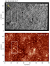 |
Fig. 1. Overview of the observed region in Hβ blue wing (top) and SJI 1400 (bottom). The white rectangle marks the region used for studying the QSEBs and UV brightenings. Red contours in the top panel denote the QSEB detections. The dark elongated thread-like features are spicules. Inside Region 1, a spicule is visible close to the QSEB, shown by a white arrow, which later becomes part of an inverted-Y-shaped jet as discussed in Sect. 4.1. Yellow contours in the bottom panel represent the detected > 5σ UV brightenings. The yellow arrow in the top panel shows the direction towards the north limb. |
3.2. Magnetic field extrapolation
To infer the magnetic field topology associated with the QSEB events, we applied fast Fourier transformation (FFT) based potential field extrapolations (Nakagawa & Raadu 1972; Alissandrakis 1981) on Region 1 using the photospheric BLOS data from SST. The extrapolation is performed over a box size of 256 × 512 × 256 grid points, approximately corresponding to a physical domain size of 7 Mm × 14 Mm × 7 Mm in the x, y, and z directions, respectively. The bottom boundary for extrapolation was selected to ensure flux balance, allowing the resultant extrapolated magnetic field to closely satisfy the divergence-free condition. The mean value of BLOS for this region is 0.66 G, which is much lower than the noise level of 6.4 G in BLOS. The ratio of the total flux to the total unsigned flux in this case is 0.09. The extrapolated magnetic field lines were visualised in 3D using the VAPOR software (Li et al. 2019). The VAPOR software allows us to trace the magnetic field lines near the base of the QSEB through bidirectional field line integration by randomly placing the seed points with a bias towards higher values of |BLOS|. This allows us to continuously follow the strong polarities in a small region close to the QSEB as they move during the time series. We further calculated the squashing factor Q (Titov et al. 2002, 2009) for the extrapolated magnetic field using the code by Liu et al. (2016). This allowed us to locate the magnetic null points by biasing the seed points with a large squashing factor, and follow the changes in fan-spine topology associated with the 3D null points during the event. To visually compare the 3D magnetic field lines with QSEBs in the Hβ wing and UV brightenings in the SJI 1400 Å channel, we have placed the Hβ layer in a plane close to the photosphere, while the SJI 1400 layer is placed at different heights depending on the 3D null’s location.
4. Results
This study presents two scenarios where QSEBs and associated UV brightenings arise due to interaction between the fan surfaces of two 3D nulls. In the first case, the fan surface of one 3D null resides inside a larger fan surface of another 3D null. In the second case, the two fan surfaces are situated side by side, with a small region of overlap. In both cases, we observe chromospheric inverted-Y-shaped jets originating close to the QSEBs where the fan surfaces of the two 3D nulls interact. In the following subsections, we present observations and magnetic field extrapolations illustrating these cases.
4.1. Nested fan-spine topologies
Here, we study two QSEBs events associated with two nested 3D nulls with a UV brightening observed close to the outer 3D null. The potential field extrapolation for this region is shown in Fig. 2, which illustrates the nested fan-spine topologies. The inner fan-spine configuration (3D null 2) is located inside an outer fan-spine configuration (3D null 1). This configuration is also shown at a different viewing angle, at the same instance in Fig. 3a. The fan surfaces of both the 3D nulls are clustered in regions of local magnetic field concentrations coinciding with the location of the two QSEBs. These two QSEBs, designated as QSEB-A and QSEB-B, are visible in Fig. 3a, which depicts an instance when both QSEBs occur simultaneously. QSEB-A starts at 08:28:43 UT and ends at 08:29:55 UT, lasting for a duration of 72 s, while QSEB-B begins at 08:29:12 UT and ends at 08:31:13 UT with a duration of 121 s. Notably, the UV brightening occurs close to the outer 3D null point and is situated 660 km above the photosphere in Fig. 3a. This UV brightening is the same as the one previously discussed in Section 4.3 of Paper II. For the sake of completeness, here we briefly summarise this scenario from Section 4.3 of Paper II that included an observation of a UV brightening occurring close to the 3D null 1, and the QSEB being situated close to the footpoints of the fan surface having a local concentration of strong magnetic field. The QSEB was also associated with a dipolar flux-concentration whose positive footpoint was located on the same polarity as that of the fan surface footpoints. There, the QSEB and UV brightening were likely caused by a common reconnection process due to the formation of a quasi-separatrix layer (QSL) between the emerging dipole and the fan surface. In the present study, we continue following the evolution of this same region. The event occurs approximately 3 min after the one described in Section 4.3 of Paper II, where now instead of an emerging dipole we have an emerging 3D null with fan-spine topology. We now observe two QSEBs: QSEB-A and QSEB-B, at the footpoints of the initial fan-spine configuration. The UV brightening continues from the previous event and likely occurs due to the formation of QSLs between the emerging fan surface and the already existing outer fan surface.
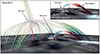 |
Fig. 2. Two nested fan-spine magnetic field topologies obtained from potential field extrapolation. A smaller fan-spine structure (3D null 2) is located inside the fan surface of the larger one (3D null 1). The two fan surfaces share footpoints at two positive polarities, this is shown at a different angle in Fig. 3. QSEB-B is located at one of the shared footpoints of the fan-surfaces, shown in light blue and white shades in the Hβ –0.6 Å image placed close to the photosphere. The inset shows the zoom-in of 3D null 2 at a slightly different angle to clearly highlight the fan-spine configuration. The yellow arrow points to the direction of the north solar limb. |
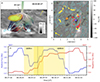 |
Fig. 3. Magnetic field topology of a smaller fan-spine structure inside a bigger fan-spine structure. Panel (a) shows the nested topology with the UV brightening in yellow colour located close to the 3D null point associated with the bigger fan-spine topology. The spines of both fan-spine structures are rooted in different negative polarity patches. The QSEBs are shown in light blue and white shades in Hβ –0.6 Å image placed close to the photosphere. Two QSEBs, namely QSEB-A and QSEB-B occur at two positive polarity patches, which are the shared footpoints of both the fan surfaces. Panel (b) shows the BLOS map with contours at 1σ above the noise level with different markers: orange cross markers denote the inner spine footpoint of 3D null 1 and yellow circles denote the footpoints of its fan surface. The blue crosses denote the position of the inner spine footpoint of 3D null 2, and the red circles show the footpoints of its fan surface. The red circles on the shared negative polarity denote the outer spine footpoint of the 3D null 2 (around x, y = 3″, 3″). The location of QSEB-A is marked with a white star, while the location of QSEB-B is marked with a blue star. The dashed pink rectangle shows the area used for calculating the magnetic flux shown in panel (c). The yellow arrows in the top panels show the direction towards the north limb. Panel (c) shows the variation of a positive and negative magnetic flux during the evolution of QSEBs and the inverted-Y-shaped jet. The error bands in positive and negative fluxes are shown as thin-shaded regions along the curves. The yellow-shaded regions denote the period of occurrence of QSEB-A and QSEB-B. The vertical dashed lines denote the start and end of the inverted-Y-shaped jet. |
Figure 3b marks the footpoints of field lines close to the inner spines and fan surfaces of the two 3D null points, as well as the locations of the QSEBs on the BLOS map. The dashed pink box outlines a region containing the two stronger positive polarity patches, where the QSEBs are located. Figure 3c shows the evolution of positive and negative magnetic flux in this region. We notice that an episode of flux emergence starts around 08:29:05 UT. The positive flux then begins to decrease from 08:30:37 UT, although the negative flux continues to increase, suggesting possible cancellation along with flux emergence.
The two dashed vertical lines in Fig. 3c mark the start and end of a chromospheric inverted-Y-shaped jet that originates close to the two QSEBs. Figure 4 illustrates different stages of this inverted-Y-shaped jet in different wavelength positions of the Hβ line at different times. During the evolution, we observe the presence of two strands and a spire of chromospheric material. Notably, the jet is visible in the blue wing of the Hβ spectral line, implying that these are related to possible reconnection outflows, or similar to RBEs. The inverted-Y-shaped jet originates as a single strand (Strand 1) at 08:29:33 UT and is visible in Fig. 4b, which displays the blue wing image at 08:30:16 UT. Figure 1 also depicts the Hβ FOV at this time, in which the QSEB and the strand are visible inside the white rectangle. The strand looks quite similar to the other spicules (RBEs), which are dark, elongated, thread-like structures in the image. This strand originates close to QSEB-B, at coordinates ( ) as shown in Fig. 3b. From the online movie, it can be seen that this strand bends at its top around 08:30:30 UT. Another strand (Strand 2) appears slightly later, at 08:30:23 UT, from the location of QSEB-A. Both of the strands originate during the flux emergence episode shown in Fig. 3c. The two strands meet at 08:30:30 UT, which is shown in panel (c) at 08:30:52 UT. Figure 4d shows the spire of the jet in the core of the Hβ line at 08:30:52 UT. This spire is visible in the Hβ core from 08:29:48 UT. Figure 4e shows the two strands converged at the base of the spire at 08:31:06 UT, which then resembles the inverted-Y-shaped jet. After the strands meet, we also observe some brightening in the Hβ core just below their point of intersection. This brightening is shown in Fig. 4e at 08:31:06 UT, and lasts for 28 s from 08:30:52 UT to 08:31:20 UT. As the jet rises upwards in the Hβ core, the brightening below their point of intersection also moves up with the jet. The jet fades after 08:31:28 UT across all the wavelength positions of the Hβ spectral line. Additionally, another brief brightening is detected near the midpoint of the two QSEBs, which is shown in Fig. 4f in the Hβ –0.2 Å image. This brightening is short-lived and is visible from 08:30:59 UT to 08:31:06 UT. The full event, starting from the beginning of Strand 1, the merging of strands, then the brightening in the Hβ core, brightening at the footpoint to the disappearance of the inverted-Y-shaped jet, lasts for 115 s and can be seen in the corresponding online movie.
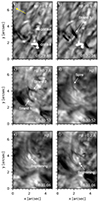 |
Fig. 4. Evolution of the inverted-Y-shaped jet with QSEBs at its footpoints. Panel (a) shows the two QSEBs in the Hβ wing. The yellow arrow points to the limb direction. Panel (b) shows the footpoints of the inverted-Y-shaped structure marked as Strand 1 and 2. Strand 1 originates close to QSEB-B and is shown in panels (b) and (c). Strand 2 starts later from the location of QSEB-A and is shown in panel (c) when it merges with Strand 1. Panel (d) shows the spire of the jet-like top part of the inverted-Y-shaped jet. Panel (e) points to the brightening in the core of the Hβ line, which occurs just below the point of intersection of the two strands, while panel (f) points to a brightening at the base of this structure. Note that the wavelength positions are different in the panels, to best show the inverted-Y-shaped jet at different instances. The QSEBs are shown only in panels (a) and (b) due to their clear visibility in the wing positions, and they fade before the jet itself dissipates. They are marked in panel (a). The full evolution of the inverted-Y-shaped jet can be viewed in the online movie. |
In the absence of electric currents in the potential field extrapolation, we use the squashing factor Q to relate the evolution of the inverted-Y-shaped jet with the magnetic topology of the region. Figure 5 shows the different stages of the inverted-Y-shaped jet alongside the logarithm of the squashing factor (log Q). Figure 5a corresponds to the same instance depicted in Figs. 3a and 4a. The magnetic field lines of the two fan surfaces converge at the same two positive polarity patches where the QSEBs A and B occur. The flux emergence along with the convective motions in the solar photosphere can cause a potential misalignment between the newly emerged inner fan-spine structure (3D null 2) and the pre-existing outer fan-spine structure (3D null 1), which could lead to the formation of QSLs and current sheets, leading to subsequent magnetic reconnections. This could be the reason for UV brightening occurring close to the 3D null 1. In the panels, we show a slice of the squashing factor Q in a plane connecting the two QSEBs, which passes through the two fan surfaces. The high Q values in this plane show a dome and spine-like contour with the footpoints of this contour connecting the positive polarity patches where the two QSEBs occur. The region with the highest Q value along a vertical high Q line in this plane is indicated with a red arrow in panel (b), where reconnection can potentially take place. The spire of the inverted-Y-shaped jet could be due to an outflow after the reconnection at this high Q region, and lie along the outer spine, which is aligned with the direction of the open magnetic field lines. Panels (b) and (c) show two instances with Strand 1 of the jet and the QSEB-B in the wings of the Hβ line. The reconnection at QSLs could trigger both the QSEB-B and Strand 1 of the jet, with QSEB occurring at the footpoint and the strand originating close to the QSEB that follows the path along the high Q contour. Panel (d) depicts Strand 2 of the jet after it merges with Strand 1 in the wings of the Hβ line. Since this strand originates from the site where QSEB-A was previously located, the cause of its occurrence is probably similar to that of Strand 1. Notably, the contour of high Q values close to QSEB-B is more extended than the one close to QSEB-A. This may explain why Strand 1 is longer compared to Strand 2 as seen in Fig. 4c. The brightening in the Hβ core just below the point of intersection of the two strands likely occurs below the reconnection site, along the high Q region, as seen in panel (e). Figure 5f points to a brightening close to the footpoint of the vertical high Q line. This footpoint coincides with the inner spine footpoint of the 3D null 2 (field lines are not shown in this panel). Since our observation is close to the north solar limb, we see the jet projected towards the direction of the limb in the Hβ images. Projection effects corresponding to a viewing angle of μ = 0.48 lead to an offset of approximately 1.78 Mm in the observed position for every 1 Mm of height in the solar atmosphere. The high Q region (shown in panel (b) with a red arrow) is situated between 660 km to 720 km from the footpoint of the inner spine. Since the two strands likely intersect at the region of high Q values, this translates to a distance of 1.1–1.2 Mm due to the projection effects. This matches with the distance of the point of intersection of the two strands in Hβ core from the footpoint of the vertical high Q line is 1.2 Mm. From the observations, we also see that the jet rises upwards in the Hβ core and fades by 08:31:28 UT. This agrees with the instance when the inner 3D null 2 is no longer present in the magnetic field extrapolations (not shown here). From panels (a) to (f) of Fig. 5, we note that the size of the Q contour keeps on increasing from 08:29:48 UT to 08:31:06 UT. The region with the highest Q values is around 386 km above the photosphere at 08:29:48 UT and rises to 720 km by 08:31:06 UT. The increase in the magnetic field strength at the negative polarity during flux emergence can explain the upward expansion of the high Q region, while the subsequent magnetic reconnection can explain the rising nature of the chromospheric inverted-Y-shaped jet.
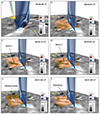 |
Fig. 5. Stages of the inverted-Y-shaped jet along with the logarithm of the squashing factor (log Q), at different instances. In all panels, the grey-scale image at the bottom is the BLOS map, while the yellow arrow points to the north limb. Panel (a) shows the magnetic field lines associated with the two 3D nulls, along with the UV brightening in yellow close to the outer 3D null and the QSEBs at the fan surface footpoints. The magnetic field lines are not shown in other panels to avoid clutter. All panels include log Q slices, where red indicates high Q values. The red arrow in panel (b) points to the region with the highest value along a vertical high Q line, where reconnection likely occurs. A brown layer in panels (b)–(f) shows the Hβ image at different wavelengths, which depict the various features of the inverted-Y-shaped jet. The dashed black arrow in panel (e) marks the distance between the vertical high Q line and the merging strands (1.2 Mm). |
4.2. Adjacent fan-spine topologies
In this section, we present a scenario involving two fan-spine structures corresponding to two null points (3D nulls 1 and 3) that are adjacent to one another. A QSEB (QSEB-C) is located at a shared polarity patch where both the fan surface footpoints are situated. This magnetic field configuration is shown in Fig. 6a. About 3 min after QSEB-A, the positive polarity associated with it in Sect. 4.1 moves slightly towards the north, likely due to convection, and QSEB-C is later observed at this polarity. QSEB-C is still located at the footpoints of the 3D null 1 discussed in the previous section, although the inner fan-spine structure (3D null 2) does not exist any more. QSEB-C is highlighted with a different colour as compared to previous figures for better visibility among the large number of magnetic field lines shown in the panel. We also observe a UV brightening close to the 3D null 1 on the left, which has been persistent since the start of QSEB-A and is highlighted in yellow near the null 1 in panel (a). The height of the 3D null 1 has increased to 860 km since the previous event, while the 3D null 3 is located 1012 km above the photosphere. Panel (b) highlights the footpoints of the two fan surfaces, along with the position of the footpoints of their inner spines, and the QSEB marker at the intersection of the fan surfaces. In panel (a), we have shown the logarithm of the squashing factor log Q at a height close to the photosphere. We notice a region of high Q (in red), below the QSEB, above the shared polarity of the two fan-spine topologies. The high Q region persists for the whole duration of the QSEB, suggesting the probable formation of the QSLs at the intersection of fan surfaces, which likely causes current sheets formation and drives the QSEB activity. For this case, it was difficult to calculate the magnetic flux as the two fan-spine structures cover a large area and involve many positive polarities, which are not associated with the QSEB. We also observe the formation of a chromospheric inverted-Y-shaped jet, emerging from this QSEB. The various stages of this jet are illustrated in Fig. 7, which shows six instances at different times and wavelength positions in the wings of the Hβ line. QSEB-C begins at 08:32:46 UT and at the same time, Strand 1 of the jet starts to appear close to the QSEB, depicted in Fig. 7a. Strand 2 forms at 08:33:57 UT, and shortly afterwards, the spire becomes visible, extending towards the direction of the limb, and completing the inverted-Y-shaped jet. In this case, we were not able to isolate the magnetic field structures associated with the strands, as it is likely that these structures form as a result of the interaction between the fan surfaces and are missing in the potential field extrapolation. QSEB-C persists for 164 s, ending at 08:35:31 UT. Unlike the previous case, the jet in this case appears to fall down and fades by 08:37:04 UT, lasting for 258 s. An accompanying movie also shows the evolution of the QSEB and the jet.
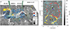 |
Fig. 6. Magnetic field topology showing two adjacent fan-spine structures. The 3D null 1 shown here is the same as in Fig. 3. The UV brightening is located close to the 3D null 1. The inner spines of the two 3D nulls are rooted in different negative polarity patches, with their fan footpoints at nearby positive polarities. The QSEB is shown in yellow colour in Hβ –0.6 Å image for better visibility among a large number of magnetic field lines. QSEB-C is located at the shared fan surface footpoints of both the 3D nulls. Panel (b) shows the BLOS map with contours at 2σ above the noise level with different markers: orange cross markers denote the inner spine footpoint of the 3D null 1 and yellow circles denote the footpoints of its fan surface. The blue crosses denote the position of the inner spine footpoint of the 3D null 3, and the red circles show the footpoints of its fan surface. The location of QSEB-C is marked with a blue star. The log Q plane is displayed close to the photosphere, where regions in red denote high values of Q. Yellow arrows in both panels show the direction towards the limb. |
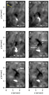 |
Fig. 7. Evolution of the inverted-Y-shaped jet alongwith QSEB-C of Fig. 6 at one of its footpoints. The footpoints of the inverted-Y-shaped structure are marked as Strand 1 and 2. Panel (a) shows the QSEB in the Hβ wing, along with the beginning of Strand 1 of the inverted-Y-shaped jet, which originates very close to the QSEB. Both the QSEB and Strand 1 begin at the same time. Panels (b) and (c) show the progress of QSEB and the strand. Strand 2 starts to develop in panel (c) but is clearly visible in panels (d), (e) and (f). The merged strands with the spire of the inverted-Y-shaped jet are visible in panels (d), (e) and (f). The yellow arrow in panel (a) points to the limb direction. Note that the wavelength positions are different in the panels, to best show the inverted-Y-shaped jet at different instances. The full evolution of the inverted-Y-shaped jet can be viewed in the online movie. |
5. Discussion
This study investigates scenarios involving the interaction between two fan-spine topologies that are associated with QSEBs, UV brightenings, and chromospheric inverted-Y-shaped jets. The QSEBs are studied using the Hβ data from the SST/CHROMIS instrument, and are detected using the k-means clustering algorithm. The UV brightenings are identified from the IRIS SJI 1400 data, using a threshold of 5σ above the median. Potential field extrapolations were performed on the high-resolution magnetograms from SST to study the evolution of the magnetic field topology in these regions. Our observation region is a coronal hole close to the north limb, hence the magnetic field extrapolations are done using only the line of sight magnetic field, due to substantial noise in the transverse field components (Bx and By) and projection effects. The limitations of the dataset and methods have been carefully discussed in detail in Paper II and are summarised in the following section.
5.1. Limitations
In this section, we briefly discuss the limitations of our methodology and their implications for the results presented in this study. Our analysis is based on observations of a quiet Sun region, which is characterised by relatively weak magnetic fields. This region is located near the northern limb and hence has significant projection effects when comparing features across different heights. Due to these reasons, the measurements of the local transverse magnetic field components (Bx and By), which are derived from the Stokes Q and U profiles, were noisy. This made it difficult to resolve the 180° ambiguity and accurately obtain the vector magnetic field. To mitigate these issues, we based our extrapolations solely on the line-of-sight magnetic field (BLOS), which is derived from Stokes V, and performed a potential field extrapolation without correcting for projection effects. The assumption of absence of electric currents in potential field approximation is a reasonable approximation for quiet Sun regions (except near the reconnection sites), where weaker magnetic fields give rise to relatively small currents. Our analysis was based on identifying null points and analysing their connectivity. Although we understand that the location of a null point can vary depending on the extrapolation method and null-detection algorithm used, we believe that the fan-spine topology is quite robust, and for our purposes, only the overall structure is important and not the exact location. Longcope & Parnell (2009) demonstrated that potential field extrapolations can accurately locate these structures.
5.2. Discussion of the topologies
As context, in Paper II we have shown, through a combination of observations and magnetic field modelling, that within a fan-spine configuration, a UV brightening can be observed close to the 3D null point and QSEBs can potentially be found at three different locations: (i) near the footpoint of the inner spine, (ii) near the footpoint of the outer spine, and (iii) near the footpoints of the fan surface. In Sect. 4.3 of Paper II, we presented an observation of a UV brightening occurring close to a 3D null point, and the QSEB happening close to the footpoints of the fan surface having a local concentration of strong magnetic field.
We suggested that the QSEB and UV brightening were likely caused by a common reconnection process due to the formation of a QSL between the emerging dipole of the QSEB and the fan surface. In this work, we revisit Region 1 from Paper II (now considering a larger FOV), which contains multiple recurrent QSEBs and associated UV brightenings that occur close to the 3D null point. The UV brightening discussed in Sect. 4.1 follows a similar scenario, but instead of an emerging dipole, we have an emerging 3D null with a fan surface. The same UV brightening persists (at the 3D null 1) for the event studied in Sect. 4.2.
In Sect. 4.1, we find that flux emergence leads to the formation of an inner-fan-spine topology inside the outer fan-spine topology. We also observe two QSEBs associated with this nested fan-spine configuration. The QSEBs are situated at the two shared polarities where the footpoints of the fan surfaces are located. A chromospheric inverted-Y-shaped jet also occurs, with the strands rooted close to the QSEBs. These small-scale events are likely driven by the formation of current sheets between the misaligned magnetic field lines of the two fan surfaces, leading to magnetic reconnection. We have found a similar scenario in the 2D numerical experiment by Nóbrega-Siverio & Moreno-Insertis (2022) using the Bifrost code (Gudiksen et al. 2011). The simulation was initiated using a null configuration obtained from potential field extrapolation of a prescribed distribution at the bottom boundary. Though not directly based on the current observations, we refer to this experiment for illustration purposes to show that such scenarios of nested nulls can arise due to flux emergence following magnetic buoyancy instabilities like magnetic Rayleigh-Taylor instability (Acheson 1979; Cheung & Isobe 2014) or the Parker instability (Nozawa et al. 1992; Miyagoshi & Yokoyama 2004; Isobe et al. 2007). In this simulation, a small-scale flux emergence episode self-consistently took place inside the fan of a large fan-spine topology whose null point was located at coronal heights. This event is illustrated in Fig. 8 through maps of temperature, density, magnetic field, and characteristic length. The evolution of the magnetic field in panel Fig. 8c (also see accompanying movie) reveals the presence of a bald patch (Titov et al. 1993) at x = 33 Mm and t = 43 min. Bald patches are topologically significant features, as they can lead to current sheet formation and, depending on the evolution, serve as precursors to null points with a fan-spine configuration (Müller & Antiochos 2008). In the simulation, the bald patch collapses and evolves into a null point through plasmoid-mediated reconnection. Although this is not a one-to-one match with the observations, it highlights how reconnection can be triggered within a fan-spine structure following flux emergence. The characteristic length (Nóbrega-Siverio et al. 2016), which is defined as  , facilitates the identification of the current sheet associated with the large fan spine and the one associated with the small-scale flux emergence beneath the large fan. In the latter, magnetic reconnection heats the chromospheric plasma, increasing the temperature by several hundreds of K, and launches a chromospheric inverted-Y-shaped ejection. The vertical current sheet is located at x = 32.5 Mm in Fig. 8d. This event serves as a larger-scale version that resembles the observational scenario presented in Sect. 4.1, where the reconnection could explain the QSEB in the lower atmosphere. The increased temperature that resulted from the reconnection could be sufficient to produce enhanced Hβ wing emission that would be observed as a QSEB. Figure 8b shows the strands and spire of the inverted-Y-shaped jet in the simulation, with Strand 2 originating along the current sheet that could lead to a QSEB. The accompanying movie highlights an additional current sheet near x = 36.5 Mm up to t = 44 min where another QSEB could be located, and where the Strand 1 seems to be rooted at t = 51.33 min.
 |
Fig. 8. Chromospheric inverted-Y-shaped jet from the numerical experiment by Nóbrega-Siverio & Moreno-Insertis (2022). The panels show, from left to right: the temperature, T; the mass density, ρ; the magnetic field strength, B, with superimposed magnetic field lines; and the inverse of the characteristic length of the magnetic field, L |

To further investigate the magnetic field configuration present in our 2D numerical simulation and its resemblance to the observations in greater detail, we show Fig. 9. This figure displays the magnetic field lines for the same simulation timestep as shown in Fig. 8, and highlights the nested null scenario similar to Fig. 2. Additionally, the rectangular inset zooms on the inner null where plasmoid-mediated magnetic reconnection could result in enhanced temperatures, causing the formation of a QSEB.
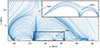 |
Fig. 9. Detailed view of the magnetic field configuration from the 2D simulation at t = 51.33 min (corresponding to Fig. 8), showing the nested null configuration (with null 2 inside the fan of null 1). The rectangular inset shows a zoomed view of the magnetic structure around null 2, where only the relevant field lines are plotted for clarity. |
In Sect. 4.2, we present a configuration where there are two 3D nulls adjacent to each other, and we observe the QSEB and the chromospheric inverted-Y-shaped jet from the location where the footpoints of their fan surfaces intersect. We find a high squashing factor at the location of the QSEB for its entire duration. A similar scenario of interaction between two adjacent fan surfaces has been studied by Kumar et al. (2021) using 3D MHD simulations with the EULAG-MHD code (Smolarkiewicz & Charbonneau 2013). The initial magnetic field in their simulation is shown to have QSLs in regions where the footpoints of the two fan surfaces interact. During the MHD evolution, self-consistent flows generated by the initial Lorentz forces produce rotational flows around the fan surfaces. This leads to the formation of current sheets due to the misalignment of field lines and triggers torsional fan reconnection (Priest & Pontin 2009) at the QSL locations.
The chromospheric inverted-Y-shaped jets in both scenarios of our study resemble in morphology the chromospheric anemone jets described by Shibata et al. (2007) observed in the Ca II H line in SOT/Hinode data. These jets were believed to occur as a result of magnetic reconnection between an emerging magnetic dipole and the pre-existing magnetic field. The reconnection process in Sect. 4.1 appears to follow a similar mechanism, with the chromospheric jet originating at the QSLs formed between the emerging fan and the pre-existing fan-spine topology. The jet fades once the emerging inner fan structure dissipates. The size of the cusp formed from the merged strands in our examples varies between 1″–2″, which is similar to the size 1″–3″ reported for Hinode chromospheric anemone jets by Nishizuka et al. (2011). The width of the jets in our examples is approximately  , and the height varies between 1″–2″. It has also been speculated that the footpoints of these anemone jets could correspond to EBs (Morita et al. 2010).
Y-shaped jets on scales comparable to those of our examples have also been reported by Chitta et al. (2023) in coronal hole EUV observations from Solar Orbiter, and by Yurchyshyn et al. (2011) in the intergranular lanes in the wings of the Hα line. They have also been observed in He I 10 830 Å by Wang et al. (2021) who noted bright kernels at the base of the jet which is larger in scale compared to our example. They studied the magnetic topology using nonlinear force-free field (NLFFF) extrapolations and suggested that the magnetic reconnection around QSL associated with a bald patch is the cause of the jet. They also showed that the dome and spire of the jet lie along a region of high squashing factor, consistent with our first example in Sect. 4.1. We also observe similar brightenings, one below the intersection of the jet strands and another at the footpoint of the inner spine of the smaller 3D null.
The jets in this work originate next to the QSEBs and are visible in the blue wing of the Hβ wavelength, so they could be similar upflows as the RBEs, which are the on-disc counterparts of the Type II spicules. Figure 1 shows that the strand associated with the jet discussed in Sect. 4.1 looks like the spicules in the FOV. From the evolution of this strand, we see that it bends and joins to the spire of the jet. Yurchyshyn et al. (2013) have shown using potential field extrapolations that some of the RBEs could arise due to magnetic reconnection. They suggest that the RBEs bend above the reconnection site, and also display a brightening below the bending point. Recently, Sand et al. (2025) demonstrated that a subset of the Type II spicules in their observations are rooted at QSEB locations. As a result, QSEBs and spicules reflect the conversion of magnetic energy into thermal and kinetic energy, respectively.
To conclude, in this paper, we have demonstrated, through observational and modelling evidence, how small-scale dynamic phenomena – such as QSEBs, UV brightenings, and chromospheric inverted-Y-shaped jets – are interconnected and arise from a common magnetic reconnection scenario of interacting fan-spine topologies.
Data availability
Movies associated to Figs. 4, 7, 8 are available at https://www.aanda.org
Acknowledgments
We thank Guillaume Aulanier, Reetika Joshi and Carlos José Díaz Baso for the helpful discussions. A.P. also thanks Sanjay Kumar for the helpful discussions. The Swedish 1-m Solar Telescope (SST) is operated on the island of La Palma by the Institute for Solar Physics of Stockholm University in the Spanish Observatorio del Roque de los Muchachos of the Instituto de Astrofísica de Canarias. The SST is co-funded by the Swedish Research Council as a national research infrastructure (registration number 4.3-2021-00169). This research is supported by the Research Council of Norway, project number 325491, and through its Centres of Excellence scheme, project number 262622. IRIS is a NASA small explorer mission developed and operated by LMSAL, with mission operations executed at NASA Ames Research Center and major contributions to downlink communications funded by ESA and the Norwegian Space Agency. SDO observations are courtesy of NASA/SDO and the AIA science teams. J.J. is grateful for travel support under the International Rosseland Visitor Programme. J.J. acknowledges funding support from the SERB-CRG grant (CRG/2023/007464) provided by the Anusandhan National Research Foundation, India. A.P. and D.N.S acknowledge support from the European Research Council through the Synergy Grant number 810218 (“The Whole Sun”, ERC-2018-SyG). D.N.S. also acknowledges the computer resources at the MareNostrum supercomputing installation and the technical support provided by the Barcelona Supercomputing Center (BSC, RES-AECT-2021-1-0023, RES-AECT-2022-2-0002), as well as the resources provided by Sigma2 – the National Infrastructure for High Performance Computing and Data Storage in Norway. We acknowledge using the visualisation software VAPOR (www.vapor.ucar.edu) for generating relevant graphics. We made much use of NASA’s Astrophysics Data System Bibliographic Services.
References
- Acheson, D. J. 1979, Sol. Phys., 62, 23 [Google Scholar]
- Alissandrakis, C. E. 1981, A&A, 100, 197 [NASA ADS] [Google Scholar]
- Bhatnagar, A., Rouppe van der Voort, L., & Joshi, J. 2024, A&A, 689, A156 [NASA ADS] [CrossRef] [EDP Sciences] [Google Scholar]
- Bhatnagar, A., Prasad, A., Rouppe van der Voort, L., Nóbrega-Siverio, D., & Joshi, J. 2025, A&A, 693, A221 [NASA ADS] [CrossRef] [EDP Sciences] [Google Scholar]
- Bose, S., Henriques, V. M. J., Joshi, J., & Rouppe van der Voort, L. 2019, A&A, 631, L5 [NASA ADS] [CrossRef] [EDP Sciences] [Google Scholar]
- Bose, S., Nóbrega-Siverio, D., De Pontieu, B., & Rouppe van der Voort, L. 2023, ApJ, 944, 171 [NASA ADS] [CrossRef] [Google Scholar]
- Chen, Y., Tian, H., Peter, H., et al. 2019, ApJ, 875, L30 [NASA ADS] [CrossRef] [Google Scholar]
- Cheung, M. C. M., & Isobe, H. 2014, Liv. Rev. Sol. Phys., 11, 3 [Google Scholar]
- Chitta, L. P., Peter, H., Young, P. R., & Huang, Y. M. 2017, A&A, 605, A49 [NASA ADS] [CrossRef] [EDP Sciences] [Google Scholar]
- Chitta, L. P., Zhukov, A. N., Berghmans, D., et al. 2023, Science, 381, 867 [NASA ADS] [CrossRef] [Google Scholar]
- de la Cruz Rodríguez, J. 2019, A&A, 631, A153 [NASA ADS] [CrossRef] [EDP Sciences] [Google Scholar]
- de la Cruz Rodríguez, J., Löfdahl, M. G., Sütterlin, P., Hillberg, T., & Rouppe van der Voort, L. 2015, A&A, 573, A40 [NASA ADS] [CrossRef] [EDP Sciences] [Google Scholar]
- Demoulin, P., Henoux, J. C., Priest, E. R., & Mandrini, C. H. 1996, A&A, 308, 643 [NASA ADS] [Google Scholar]
- De Pontieu, B., Hansteen, V. H., Rouppe van der Voort, L., van Noort, M., & Carlsson, M. 2007a, ApJ, 655, 624 [Google Scholar]
- de Pontieu, B., McIntosh, S., Hansteen, V. H., et al. 2007b, PASJ, 59, S655 [NASA ADS] [CrossRef] [Google Scholar]
- De Pontieu, B., Title, A. M., Lemen, J. R., et al. 2014, Sol. Phys., 289, 2733 [Google Scholar]
- Ellerman, F. 1917, ApJ, 46, 298 [NASA ADS] [CrossRef] [Google Scholar]
- Everitt, B. S. 1972, Br. J. Psychiatry, 120, 143 [Google Scholar]
- Georgoulis, M. K., Rust, D. M., Bernasconi, P. N., & Schmieder, B. 2002, ApJ, 575, 506 [Google Scholar]
- Gudiksen, B. V., Carlsson, M., Hansteen, V. H., et al. 2011, A&A, 531, A154 [NASA ADS] [CrossRef] [EDP Sciences] [Google Scholar]
- Gupta, G. R., & Tripathi, D. 2015, ApJ, 809, 82 [Google Scholar]
- Hansteen, V. H., De Pontieu, B., Rouppe van der Voort, L., van Noort, M., & Carlsson, M. 2006, ApJ, 647, L73 [Google Scholar]
- Hansteen, V. H., Archontis, V., Pereira, T. M. D., et al. 2017, ApJ, 839, 22 [NASA ADS] [CrossRef] [Google Scholar]
- Hansteen, V., Ortiz, A., Archontis, V., et al. 2019, A&A, 626, A33 [NASA ADS] [CrossRef] [EDP Sciences] [Google Scholar]
- Hashimoto, Y., Kitai, R., Ichimoto, K., et al. 2010, PASJ, 62, 879 [NASA ADS] [Google Scholar]
- Huang, Z., Madjarska, M. S., Scullion, E. M., et al. 2017, MNRAS, 464, 1753 [NASA ADS] [CrossRef] [Google Scholar]
- Isobe, H., Miyagoshi, T., Shibata, K., & Yokoyama, T. 2007, in New Solar Physics with Solar-B Mission, eds. K. Shibata, S. Nagata, & T. Sakurai, Astronomical Society of the Pacific Conference Series, 369, 355 [Google Scholar]
- Joshi, J., & Rouppe van der Voort, L. H. M. 2022, A&A, 664, A72 [NASA ADS] [CrossRef] [EDP Sciences] [Google Scholar]
- Joshi, J., Rouppe van der Voort, L. H. M., & de la Cruz Rodríguez, J. 2020, A&A, 641, L5 [EDP Sciences] [Google Scholar]
- Kleint, L., & Panos, B. 2022, A&A, 657, A132 [NASA ADS] [CrossRef] [EDP Sciences] [Google Scholar]
- Kosugi, T., Matsuzaki, K., Sakao, T., et al. 2007, Sol. Phys., 243, 3 [Google Scholar]
- Kumar, S., Nayak, S. S., Prasad, A., & Bhattacharyya, R. 2021, Sol. Phys., 296, 26 [Google Scholar]
- Kurokawa, H., Kawaguchi, I., Funakoshi, Y., & Nakai, Y. 1982, Sol. Phys., 79, 77 [NASA ADS] [CrossRef] [Google Scholar]
- Langangen, Ø., De Pontieu, B., Carlsson, M., et al. 2008, ApJ, 679, L167 [Google Scholar]
- Li, S., Jaroszynski, S., Pearse, S., Orf, L., & Clyne, J. 2019, Atmosphere, 10, 488 [NASA ADS] [CrossRef] [Google Scholar]
- Liu, R., Kliem, B., Titov, V. S., et al. 2016, ApJ, 818, 148 [Google Scholar]
- Löfdahl, M. G., Hillberg, T., de la Cruz Rodríguez, J., et al. 2021, A&A, 653, A68 [Google Scholar]
- Longcope, D. W. 2005, Liv. Rev. Sol. Phys., 2, 7 [Google Scholar]
- Longcope, D. W., & Parnell, C. E. 2009, Sol. Phys., 254, 51 [NASA ADS] [CrossRef] [Google Scholar]
- Martínez-Sykora, J., De Pontieu, B., Carlsson, M., et al. 2017a, ApJ, 847, 36 [Google Scholar]
- Martínez-Sykora, J., De Pontieu, B., Hansteen, V. H., et al. 2017b, Science, 356, 1269 [Google Scholar]
- Martínez-Sykora, J., Leenaarts, J., De Pontieu, B., et al. 2020, ApJ, 889, 95 [Google Scholar]
- Miyagoshi, T., & Yokoyama, T. 2004, ApJ, 614, 1042 [NASA ADS] [CrossRef] [Google Scholar]
- Morita, S., Shibata, K., UeNo, S., et al. 2010, PASJ, 62, 901 [Google Scholar]
- Müller, D. A. N., & Antiochos, S. K. 2008, Ann. Geophys., 26, 2967 [CrossRef] [Google Scholar]
- Nakagawa, Y., & Raadu, M. A. 1972, Sol. Phys., 25, 127 [NASA ADS] [CrossRef] [Google Scholar]
- Nelson, C. J., Scullion, E. M., Doyle, J. G., Freij, N., & Erdélyi, R. 2015, ApJ, 798, 19 [Google Scholar]
- Nelson, C. J., Freij, N., Reid, A., et al. 2017, ApJ, 845, 16 [Google Scholar]
- Nindos, A., & Zirin, H. 1998, Sol. Phys., 182, 381 [NASA ADS] [CrossRef] [Google Scholar]
- Nishizuka, N., Shimizu, M., Nakamura, T., et al. 2008, ApJ, 683, L83 [NASA ADS] [CrossRef] [Google Scholar]
- Nishizuka, N., Nakamura, T., Kawate, T., Singh, K. A. P., & Shibata, K. 2011, ApJ, 731, 43 [Google Scholar]
- Nóbrega-Siverio, D., & Moreno-Insertis, F. 2022, ApJ, 935, L21 [CrossRef] [Google Scholar]
- Nóbrega-Siverio, D., Moreno-Insertis, F., & Martínez-Sykora, J. 2016, ApJ, 822, 18 [Google Scholar]
- Nóbrega-Siverio, D., Martínez-Sykora, J., Moreno-Insertis, F., & Rouppe van der Voort, L. 2017, ApJ, 850, 153 [CrossRef] [Google Scholar]
- Nóbrega-Siverio, D., Cabello, I., Bose, S., et al. 2024, A&A, 686, A218 [NASA ADS] [CrossRef] [EDP Sciences] [Google Scholar]
- Nozawa, S., Shibata, K., Matsumoto, R., et al. 1992, ApJS, 78, 267 [NASA ADS] [CrossRef] [Google Scholar]
- Ortiz, A., Hansteen, V. H., Nóbrega-Siverio, D., & Rouppe van der Voort, L. 2020, A&A, 633, A58 [NASA ADS] [CrossRef] [EDP Sciences] [Google Scholar]
- Pariat, E., Aulanier, G., Schmieder, B., et al. 2004, ApJ, 614, 1099 [Google Scholar]
- Pariat, E., Aulanier, G., Schmieder, B., et al. 2006, Adv. Space Res., 38, 902 [NASA ADS] [CrossRef] [Google Scholar]
- Pariat, E., Masson, S., & Aulanier, G. 2012a, in 4th Hinode Science Meeting: Unsolved Problems and Recent Insights, eds. L. Bellot Rubio, F. Reale, & M. Carlsson, Astronomical Society of the Pacific Conference Series, 455, 177 [Google Scholar]
- Pariat, E., Schmieder, B., Masson, S., & Aulanier, G. 2012b, in Understanding Solar Activity: Advances and Challenges, eds. M. Faurobert, C. Fang, & T. Corbard, EAS Publications Series, 55, 115 [Google Scholar]
- Pereira, T. M. D., Rouppe van der Voort, L., Hansteen, V. H., & De Pontieu, B. 2018, A&A, 611, L6 [NASA ADS] [CrossRef] [EDP Sciences] [Google Scholar]
- Peter, H., Tian, H., Curdt, W., et al. 2014, Science, 346, 1255726 [Google Scholar]
- Priest, E. R., & Forbes, T. G. 2002, A&ARv, 10, 313 [Google Scholar]
- Priest, E. R., & Pontin, D. I. 2009, Phys. Plasmas, 16, 122101 [Google Scholar]
- Rouppe van der Voort, L., Leenaarts, J., de Pontieu, B., Carlsson, M., & Vissers, G. 2009, ApJ, 705, 272 [Google Scholar]
- Rouppe van der Voort, L. H. M., Rutten, R. J., & Vissers, G. J. M. 2016, A&A, 592, A100 [NASA ADS] [CrossRef] [EDP Sciences] [Google Scholar]
- Rouppe van der Voort, L., De Pontieu, B., Scharmer, G. B., et al. 2017, ApJ, 851, L6 [Google Scholar]
- Rouppe van der Voort, L. H. M., De Pontieu, B., Carlsson, M., et al. 2020, A&A, 641, A146 [EDP Sciences] [Google Scholar]
- Rouppe van der Voort, L. H. M., Joshi, J., & Krikova, K. 2024, A&A, 683, A190 [NASA ADS] [CrossRef] [EDP Sciences] [Google Scholar]
- Rutten, R. J., Vissers, G. J. M., Rouppe van der Voort, L. H. M., Sütterlin, P., & Vitas, N. 2013, J. Phys.: Conf. Ser., 440, 012007 [Google Scholar]
- Samanta, T., Tian, H., Yurchyshyn, V., et al. 2019, Science, 366, 890 [NASA ADS] [CrossRef] [Google Scholar]
- Sand, M. O., Rouppe van der Voort, L. H. M., Joshi, J., et al. 2025, A&A, 697, A180 [NASA ADS] [CrossRef] [EDP Sciences] [Google Scholar]
- Scharmer, G. 2017, in SOLARNET IV: The Physics of the Sun from the Interior to the Outer Atmosphere, 85 [Google Scholar]
- Scharmer, G. B., Bjelksjo, K., Korhonen, T. K., Lindberg, B., & Petterson, B. 2003, in Innovative Telescopes and Instrumentation for Solar Astrophysics, eds. S. L. Keil, & S. V. Avakyan, Society of Photo-Optical Instrumentation Engineers (SPIE) Conference Series, 4853, 341 [NASA ADS] [CrossRef] [Google Scholar]
- Scharmer, G. B., Narayan, G., Hillberg, T., et al. 2008, ApJ, 689, L69 [Google Scholar]
- Scharmer, G. B., Sliepen, G., Sinquin, J. C., et al. 2024, A&A, 685, A32 [NASA ADS] [CrossRef] [EDP Sciences] [Google Scholar]
- Sekse, D. H., Rouppe van der Voort, L., & De Pontieu, B. 2012, ApJ, 752, 108 [Google Scholar]
- Severny, A. B. 1964, ARA&A, 2, 363 [NASA ADS] [CrossRef] [Google Scholar]
- Shibata, K., Nakamura, T., Matsumoto, T., et al. 2007, Science, 318, 1591 [Google Scholar]
- Smitha, H. N., Chitta, L. P., Wiegelmann, T., & Solanki, S. K. 2018, A&A, 617, A128 [NASA ADS] [CrossRef] [EDP Sciences] [Google Scholar]
- Smolarkiewicz, P. K., & Charbonneau, P. 2013, J. Comput. Phys., 236, 608 [NASA ADS] [CrossRef] [Google Scholar]
- Tian, H., Xu, Z., He, J., & Madsen, C. 2016, ApJ, 824, 96 [CrossRef] [Google Scholar]
- Tian, H., Zhu, X., Peter, H., et al. 2018, ApJ, 854, 174 [NASA ADS] [CrossRef] [Google Scholar]
- Titov, V. S., Priest, E. R., & Demoulin, P. 1993, A&A, 276, 564 [NASA ADS] [Google Scholar]
- Titov, V. S., Hornig, G., & Démoulin, P. 2002, J. Geophys. Res. Space Phys., 107, 1164 [NASA ADS] [CrossRef] [Google Scholar]
- Titov, V. S., Forbes, T. G., Priest, E. R., Mikić, Z., & Linker, J. A. 2009, ApJ, 693, 1029 [NASA ADS] [CrossRef] [Google Scholar]
- Toriumi, S., Katsukawa, Y., & Cheung, M. C. M. 2017, ApJ, 836, 63 [Google Scholar]
- Tsuneta, S., Ichimoto, K., Katsukawa, Y., et al. 2008, Sol. Phys., 249, 167 [Google Scholar]
- Van Noort, M., Rouppe Van Der Voort, L., & Löfdahl, M. G. 2005, Sol. Phys., 228, 191 [NASA ADS] [CrossRef] [Google Scholar]
- Vissers, G. J. M., Rouppe van der Voort, L. H. M., Rutten, R. J., Carlsson, M., & De Pontieu, B. 2015, ApJ, 812, 11 [NASA ADS] [CrossRef] [Google Scholar]
- Wang, Y., Zhang, Q., & Ji, H. 2021, ApJ, 913, 59 [NASA ADS] [CrossRef] [Google Scholar]
- Watanabe, H., Kitai, R., Okamoto, K., et al. 2008, ApJ, 684, 736 [Google Scholar]
- Watanabe, H., Vissers, G., Kitai, R., Rouppe van der Voort, L., & Rutten, R. J. 2011, ApJ, 736, 71 [NASA ADS] [CrossRef] [Google Scholar]
- Yokoyama, T., & Shibata, K. 1996, PASJ, 48, 353 [Google Scholar]
- Young, P. R., Tian, H., Peter, H., et al. 2018, Space Sci. Rev., 214, 120 [Google Scholar]
- Yurchyshyn, V. B., Goode, P. R., Abramenko, V. I., & Steiner, O. 2011, ApJ, 736, L35 [Google Scholar]
- Yurchyshyn, V., Abramenko, V., & Goode, P. 2013, ApJ, 767, 17 [NASA ADS] [CrossRef] [Google Scholar]
- Zhao, J., Schmieder, B., Li, H., et al. 2017, ApJ, 836, 52 [Google Scholar]
All Figures
|
Fig. 1. Overview of the observed region in Hβ blue wing (top) and SJI 1400 (bottom). The white rectangle marks the region used for studying the QSEBs and UV brightenings. Red contours in the top panel denote the QSEB detections. The dark elongated thread-like features are spicules. Inside Region 1, a spicule is visible close to the QSEB, shown by a white arrow, which later becomes part of an inverted-Y-shaped jet as discussed in Sect. 4.1. Yellow contours in the bottom panel represent the detected > 5σ UV brightenings. The yellow arrow in the top panel shows the direction towards the north limb. |
| In the text | |
|
Fig. 2. Two nested fan-spine magnetic field topologies obtained from potential field extrapolation. A smaller fan-spine structure (3D null 2) is located inside the fan surface of the larger one (3D null 1). The two fan surfaces share footpoints at two positive polarities, this is shown at a different angle in Fig. 3. QSEB-B is located at one of the shared footpoints of the fan-surfaces, shown in light blue and white shades in the Hβ –0.6 Å image placed close to the photosphere. The inset shows the zoom-in of 3D null 2 at a slightly different angle to clearly highlight the fan-spine configuration. The yellow arrow points to the direction of the north solar limb. |
| In the text | |
|
Fig. 3. Magnetic field topology of a smaller fan-spine structure inside a bigger fan-spine structure. Panel (a) shows the nested topology with the UV brightening in yellow colour located close to the 3D null point associated with the bigger fan-spine topology. The spines of both fan-spine structures are rooted in different negative polarity patches. The QSEBs are shown in light blue and white shades in Hβ –0.6 Å image placed close to the photosphere. Two QSEBs, namely QSEB-A and QSEB-B occur at two positive polarity patches, which are the shared footpoints of both the fan surfaces. Panel (b) shows the BLOS map with contours at 1σ above the noise level with different markers: orange cross markers denote the inner spine footpoint of 3D null 1 and yellow circles denote the footpoints of its fan surface. The blue crosses denote the position of the inner spine footpoint of 3D null 2, and the red circles show the footpoints of its fan surface. The red circles on the shared negative polarity denote the outer spine footpoint of the 3D null 2 (around x, y = 3″, 3″). The location of QSEB-A is marked with a white star, while the location of QSEB-B is marked with a blue star. The dashed pink rectangle shows the area used for calculating the magnetic flux shown in panel (c). The yellow arrows in the top panels show the direction towards the north limb. Panel (c) shows the variation of a positive and negative magnetic flux during the evolution of QSEBs and the inverted-Y-shaped jet. The error bands in positive and negative fluxes are shown as thin-shaded regions along the curves. The yellow-shaded regions denote the period of occurrence of QSEB-A and QSEB-B. The vertical dashed lines denote the start and end of the inverted-Y-shaped jet. |
| In the text | |
|
Fig. 4. Evolution of the inverted-Y-shaped jet with QSEBs at its footpoints. Panel (a) shows the two QSEBs in the Hβ wing. The yellow arrow points to the limb direction. Panel (b) shows the footpoints of the inverted-Y-shaped structure marked as Strand 1 and 2. Strand 1 originates close to QSEB-B and is shown in panels (b) and (c). Strand 2 starts later from the location of QSEB-A and is shown in panel (c) when it merges with Strand 1. Panel (d) shows the spire of the jet-like top part of the inverted-Y-shaped jet. Panel (e) points to the brightening in the core of the Hβ line, which occurs just below the point of intersection of the two strands, while panel (f) points to a brightening at the base of this structure. Note that the wavelength positions are different in the panels, to best show the inverted-Y-shaped jet at different instances. The QSEBs are shown only in panels (a) and (b) due to their clear visibility in the wing positions, and they fade before the jet itself dissipates. They are marked in panel (a). The full evolution of the inverted-Y-shaped jet can be viewed in the online movie. |
| In the text | |
|
Fig. 5. Stages of the inverted-Y-shaped jet along with the logarithm of the squashing factor (log Q), at different instances. In all panels, the grey-scale image at the bottom is the BLOS map, while the yellow arrow points to the north limb. Panel (a) shows the magnetic field lines associated with the two 3D nulls, along with the UV brightening in yellow close to the outer 3D null and the QSEBs at the fan surface footpoints. The magnetic field lines are not shown in other panels to avoid clutter. All panels include log Q slices, where red indicates high Q values. The red arrow in panel (b) points to the region with the highest value along a vertical high Q line, where reconnection likely occurs. A brown layer in panels (b)–(f) shows the Hβ image at different wavelengths, which depict the various features of the inverted-Y-shaped jet. The dashed black arrow in panel (e) marks the distance between the vertical high Q line and the merging strands (1.2 Mm). |
| In the text | |
|
Fig. 6. Magnetic field topology showing two adjacent fan-spine structures. The 3D null 1 shown here is the same as in Fig. 3. The UV brightening is located close to the 3D null 1. The inner spines of the two 3D nulls are rooted in different negative polarity patches, with their fan footpoints at nearby positive polarities. The QSEB is shown in yellow colour in Hβ –0.6 Å image for better visibility among a large number of magnetic field lines. QSEB-C is located at the shared fan surface footpoints of both the 3D nulls. Panel (b) shows the BLOS map with contours at 2σ above the noise level with different markers: orange cross markers denote the inner spine footpoint of the 3D null 1 and yellow circles denote the footpoints of its fan surface. The blue crosses denote the position of the inner spine footpoint of the 3D null 3, and the red circles show the footpoints of its fan surface. The location of QSEB-C is marked with a blue star. The log Q plane is displayed close to the photosphere, where regions in red denote high values of Q. Yellow arrows in both panels show the direction towards the limb. |
| In the text | |
|
Fig. 7. Evolution of the inverted-Y-shaped jet alongwith QSEB-C of Fig. 6 at one of its footpoints. The footpoints of the inverted-Y-shaped structure are marked as Strand 1 and 2. Panel (a) shows the QSEB in the Hβ wing, along with the beginning of Strand 1 of the inverted-Y-shaped jet, which originates very close to the QSEB. Both the QSEB and Strand 1 begin at the same time. Panels (b) and (c) show the progress of QSEB and the strand. Strand 2 starts to develop in panel (c) but is clearly visible in panels (d), (e) and (f). The merged strands with the spire of the inverted-Y-shaped jet are visible in panels (d), (e) and (f). The yellow arrow in panel (a) points to the limb direction. Note that the wavelength positions are different in the panels, to best show the inverted-Y-shaped jet at different instances. The full evolution of the inverted-Y-shaped jet can be viewed in the online movie. |
| In the text | |
|
Fig. 8. Chromospheric inverted-Y-shaped jet from the numerical experiment by Nóbrega-Siverio & Moreno-Insertis (2022). The panels show, from left to right: the temperature, T; the mass density, ρ; the magnetic field strength, B, with superimposed magnetic field lines; and the inverse of the characteristic length of the magnetic field, L |
| In the text | |
|
Fig. 9. Detailed view of the magnetic field configuration from the 2D simulation at t = 51.33 min (corresponding to Fig. 8), showing the nested null configuration (with null 2 inside the fan of null 1). The rectangular inset shows a zoomed view of the magnetic structure around null 2, where only the relevant field lines are plotted for clarity. |
| In the text | |
Current usage metrics show cumulative count of Article Views (full-text article views including HTML views, PDF and ePub downloads, according to the available data) and Abstracts Views on Vision4Press platform.
Data correspond to usage on the plateform after 2015. The current usage metrics is available 48-96 hours after online publication and is updated daily on week days.
Initial download of the metrics may take a while.