| Issue |
A&A
Volume 689, September 2024
|
|
|---|---|---|
| Article Number | A157 | |
| Number of page(s) | 21 | |
| Section | Stellar structure and evolution | |
| DOI | https://doi.org/10.1051/0004-6361/202449978 | |
| Published online | 09 September 2024 | |
An absence of binary companions to Wolf-Rayet stars in the Small Magellanic Cloud
Implications for mass loss and black hole masses at low metallicities⋆
1
Argelander-Institut für Astronomie, Universität Bonn, Auf dem Hügel 71, 53121 Bonn, Germany
2
The School of Physics and Astronomy, Tel Aviv University, Tel Aviv 6997801, Israel
3
Max-Planck-Institut für Radioastronomie, Auf dem Hügel 69, 53121 Bonn, Germany
4
Institute of Astronomy, KU Leuven, Celestijnenlaan 200D, 3001 Leuven, Belgium
5
Max Planck Institute for Astrophysics, Karl-Schwarzschild-Strasse 1, 85748 Garching, Germany
Received:
14
March
2024
Accepted:
3
June
2024
Abstract
To predict black hole mass distributions at high redshifts, we need to understand whether very massive single stars (M ≳ 40 M⊙) with low metallicities (Z) lose their hydrogen-rich envelopes, like their metal-rich counterparts, or whether a binary companion is required to achieve this. To test this, we undertook a deep spectroscopic search for binary companions of the seven known apparently single Wolf-Rayet (WR) stars in the Small Magellanic Cloud (SMC; where Z ≃ 1/5 Z⊙). For each of them, we acquired six high-quality VLT-UVES spectra spread over a time period of 1.5 years. By using the narrow N V lines in these spectra, we monitored radial velocity (RV) variations to search for binary motion. We find low RV variations of between 6 and 23 km/s for the seven WR stars, with a median standard deviation of 5 km/s. Our Monte Carlo simulations imply probabilities below ∼5% that any of our target WR stars have a binary companion more massive than ∼5 M⊙ with orbital periods of less than a year. We estimate that the probability that all our target WR stars have companions with orbital periods shorter than 10 yr is below ∼10−5 and argue that the observed modest RV variations may originate from intrinsic atmosphere or wind variability. Our findings imply that metal-poor massive stars born with M ≳ 40 M⊙ can lose most of their hydrogen-rich envelopes via stellar winds or eruptive mass loss, which strongly constrains their initial mass–black hole mass relation. We also identify two of our seven target stars (SMC AB1 and SMC AB11) as runaway stars with a peculiar RV of ∼80 km/s. Moreover, with all five previously detected WR binaries in the SMC exhibiting orbital periods of less than 20 d, a puzzling absence of intermediate-to-long-period WR binaries has emerged, with strong implications for the outcome of massive binary interactions at low metallicities.
Key words: binaries: general / stars: black holes / stars: evolution / stars: massive / stars: mass-loss / stars: Wolf-Rayet
Based on observations collected at the European Organisation for Astronomical Research in the Southern Hemisphere under ESO program 108.22M1.001.
Corresponding author; This email address is being protected from spambots. You need JavaScript enabled to view it. .
© The Authors 2024
 Open Access article, published by EDP Sciences, under the terms of the Creative Commons Attribution License (https://creativecommons.org/licenses/by/4.0), which permits unrestricted use, distribution, and reproduction in any medium, provided the original work is properly cited.
This article is published in open access under the Subscribe to Open model. This email address is being protected from spambots. You need JavaScript enabled to view it. to support open access publication.
1. Introduction
Two recent developments in observational astronomy have sparked a great interest in very massive stars (M > 40 M⊙) in the early Universe. First, the gravitational wave observatories of the LIGO/Virgo collaboration have detected black hole (BH) mergers of tens of solar masses (Abbott et al. 2016). These BHs most likely formed at low metallicities (Giacobbo et al. 2018). Second, the James Webb Space Telescope just launched a new era in observational astronomy and has already delivered spectacular discoveries of bright blue galaxies born briefly after the Big Bang (Castellano et al. 2022; Adams et al. 2023).
Very massive stars are crucial for both these topics, as they are progenitors of BH–BH mergers and drivers of galaxy evolution. One question is of particular relevance here: could very massive stars in the early Universe lose their hydrogen-rich envelopes via stellar winds? Current stellar evolution models give discrepant results (Yusof et al. 2013; Szécsi et al. 2015; Pauli et al. 2022). If winds were strong enough for this, the consequences would be (i) a limitation of the mass of BHs produced by isolated stars and (ii) the formation of isolated hot Wolf-Rayet (WR) stars, which may chemically enrich and ionize their environment. If not, massive stars in the early Universe without a binary companion would have remained massive and left behind massive BHs. For stars born more massive than 30 M⊙, wind mass loss is the major uncertainty regarding their final mass as BHs (Fryer et al. 2012). Also, massive stars in the early Universe would then probably have needed companions to become WR stars.
A one-of-a-kind environment for studying massive stars with chemical compositions similar to those in the early Universe is the Small Magellanic Cloud (SMC), where the metallicity (Z) is about five times lower than solar (Venn 1999). As a satellite galaxy of the Milky Way and only 62 kpc away (Graczyk et al. 2020), it is close enough to study individual stars. There are 12 known WR stars in the SMC. Five of them are known to have a hot and massive companion, and for the seven others previous searches did not find any companion stars (Westerlund 1964; Smith 1968; Sanduleak 1968, 1969; Breysacher & Westerlund 1978; Azzopardi & Breysacher 1979; Moffat 1982, 1988; Moffat et al. 1985; Morgan et al. 1991; Bartzakos et al. 2001; Massey & Duffy 2001; Massey 2003; Foellmi et al. 2003a; Foellmi 2004; Hainich et al. 2015; Shenar et al. 2016, 2018; Neugent et al. 2018).
To search for binary companions, (Foellmi et al. 2003a, hereafter F03) monitored the radial velocity (RV) of all the known SMC WR stars except SMC AB 12, which was discovered later (Massey 2003; Foellmi 2004) and has not yet been subjected to RV monitoring, and SMC AB8, which is the only WO-type SMC WR star and part of a binary system. F03 presented orbital solutions for the binary stars and analyzed the completeness of their study. They show that for binaries with orbital periods of up to 300 days that consist of a 10 M⊙ WR star with a 30 M⊙ companion, the projected semi-amplitude of the RV of the WR star is typically higher than 30 km/s, which is the minimum value for which they claim to be able to detect orbital motion. This threshold of 30 km/s is estimated as  , where σRV is the measurement error with a reported value of 20 km/s.
However, this does not rule out the presence of companion stars in general, since different orbital configurations that would decrease the projected orbital velocity of the WR star are possible. First, WR masses in the SMC are typically at least 20 M⊙ (Hainich et al. 2015; Shenar et al. 2016; Schootemeijer & Langer 2018) instead of the 10 M⊙ assumed by F03. Second, interaction can take place for wider binaries that have orbital periods of up to about 10 years (Sana et al. 2012). Third, the mass of the companion might be significantly lower than 30 M⊙.
Therefore, with the knowledge gathered up to now, it is possible that most or even all SMC WR stars are in binary systems, but that at least a few have escaped detection due to long orbital periods and/or relatively low-mass companions (Schootemeijer & Langer 2018). Here, we present a modern RV monitoring survey of the seven known apparently single WR stars in the SMC using data acquired with the 8-meter Very Large Telescope (VLT). These data allow us to reach solid conclusions regarding the binary status of these apparently single SMC WR stars. This provides important constraints on the ability of isolated massive stars in low-Z environments to shed their outer H-rich layers.
Our paper is organized as follows. In Sect. 2 we present the VLT data used in this study and our method for measuring RVs; the results of these measurements are shown in Sect. 3. We discuss the impact of line profile variability (LPV) on our results in Sect. 4, the sensitivity of our campaign to binary motion in Sect. 5, and other possible signatures of binary companions in Sect. 6. Finally, we discuss our findings in Sect. 7 and present our conclusions in Sect. 8.
2. Methods
2.1. Observations
We made use of high-resolution spectra taken by the Ultraviolet and Visual Echelle Spectrograph (UVES; Dekker et al. 2000) instrument of the VLT. For our monitoring program (program ID: 108.22M1.001; PI: Schootemeijer) six spectra in total were obtained in Service Mode for each of our seven targets. This was done during three semesters, between October 2021 and December 2022. We used the standard DIC 2 437+760 setting and a slit width of 1″. The ESO CPL pipeline (version 7.1.2) was used for the reduction of the spectra. The wavelength calibration was done with the standard ESO procedure that uses a thorium-argon lamp. We corrected the spectra for barycentric motion by subtracting the RV measured (as described in Sect. 2.2) for the extremely narrow Ca II interstellar absorption feature around 3970 Å. This correction also serves as wavelength calibration. As a test, we also corrected for barycentric motion using the baryCorr function from the PYASTRONOMY package PYASL (Piskunov & Valenti 2002). Both approaches provided similar results. We chose to use the interstellar Ca II method because it yielded RVs that are slightly more constant in time.
The UVES instrument splits the collected light into two arms: a blue arm and a red arm. For the blue arm, the covered wavelength range was 3730−5000 Å, the typical signal to noise ratio (S/N; per resolution element, and measured with the method of Stoehr et al. 2008) of the spectra was 40−50. The blue spectra have a resolving power of R = λ/Δλ ≈ 41 000, which translates into a bin size of Δλ = 0.03 Å around 4500 Å. The lines that we used for the RV measurements are in the wavelength range of the blue arm. The spectra taken with the red arm in the wavelength range 5660−9460 Å had a typical S/N of 25−30 and a resolving power of R ≈ 42 000.
SMC AB11 has a red source with a similar G magnitude (both have G = 15.8) 1″ away from it, causing the point spread functions of the two objects to blend. To enable a relatively clean extraction of the WR spectrum, the slit orientation for SMC AB11 was set to include both sources. The spectrum of the WR star was then extracted from the 2D spectrum image by identifying the spatial pixel beyond which the contribution of the red sources becomes negligible.
For three out of seven targeted stars – SMC AB1, 2, and 4 – archival UVES spectra from August 2006 (PI: Foellmi; see Marchenko et al. 2007) exist on the ESO archive. In their campaign, a total of 10−12 spectra was taken on two successive nights for each of these three stars. These spectra are in the wavelength range 3930−6030 Å, and they have an S/N of ∼50 at a resolving power of R ≈ 30 000.
2.2. Radial velocity measurements
We used a linear fit to the continuum to normalize our spectra (e.g., those shown in Fig. 1). First we selected a wavelength range around an absorption line of interest (e.g., 4596–4630 Å for the N V doublet shown in Fig. 2). We measured the average flux in the leftmost and rightmost 7.5% of that wavelength range. Then, we divided the observed flux by a linear fit to the average flux in the central points of these two wavelength ranges.
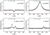 |
Fig. 1. Normalized 100 Å wide cutouts of the co-added VLT-UVES spectrum of SMC AB9. For reference, the blue arrow indicates the wavelength shift resulting from a 300 km/s velocity shift at the central wavelength of each panel. |
Our method for measuring the RV shifts of the normalized spectra is the cross-correlation method from Zucker (2003). The same method has been successfully applied to precisely measure the RVs of Galactic WR stars (Dsilva et al. 2020, 2022, 2023). We briefly describe the method below. First, the normalized spectra were shifted vertically such that the integrated flux is zero (Fig. 2, top). After that, for each of our WR stars we created a template spectrum by co-adding all available UVES spectra, starting with unshifted spectra. Then we iteratively shifted each individual spectrum by its measured RV (as described below) compared to the template spectrum, until the RVs no longer changed. After that, we calculated the cross-correlation function (CCF) between the individual spectra and the template spectrum (see the bottom panel of Fig. 2). We fitted a parabola to the CCF above 0.9 times its maximum value to obtain the best-fit RV and the statistical error σCCF; the peak of the function fitted to the CCF is the best-fit RV value and the height and width of the fit to the CCF determine the value of the statistical error.
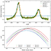 |
Fig. 2. Illustration of the cross-correlation method. Top: N V 4604, 4620 Å doublet that is used for cross-correlation, shown for SMC AB9. The co-added spectrum as well as the spectrum that was taken on observing night 0 are displayed. For reference, we also show spectrum 0 shifted by 40 km/s. The spectra are normalized and then vertically shifted such that the integrated flux in the shown wavelength range is zero. Bottom: CCFs of the N V 4604, 4620 Å doublet for the co-added template spectrum and the six individual spectra that were taken. For this figure, the spectra were not corrected for barycentric motion. |
3. Results
Figure 3 shows our RV measurements for the apparently single SMC WR stars. The time interval in days between two successive observations is written at the bottom of each panel.
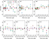 |
Fig. 3. RV measurements based on UVES spectra taken on different nights. The first of the six spectra of our observing campaign was taken on observation night 0. The time interval in days between different observation nights is written at the bottom of the subplots. For SMC AB1, 2, and 4, we also show measurements based on the preexisting UVES spectra of Marchenko et al. (2007) (they are the data from observation nights −2 and −1). In this work we opted to use the N V lines, which are shown with thicker lines. |
3.1. Best lines for radial velocity measurements
To decide on which line to use for our analysis, we show RVs from different lines in Fig. 3. The N V 4944 Å line is not observed in the relatively cold SMC WR stars AB 2 and AB 4, for which Hainich et al. (2015) found T* ≈ 45 kK, but it is detected in the spectra of the five other targeted SMC WR stars (where T* ≳ 80 kK).
Observation nights −2 and −1 in Fig. 3 refer to observations of SMC AB1, 2, and 4 of Marchenko et al. (2007), which are densely spaced on two successive nights. We notice that for these observations, the RVs measured with N V lines (both the 4604+4620 Å doublet and the line around 4944 Å) remain relatively stable. The RVs measured with He II lines are not as constant. Also for the spectra taken in our recent campaign, the RVs measured from N V lines are more stable than those from He II lines. For our seven target stars, we calculated the ΔRV (the difference between the highest and the lowest RV measurement) and the σRV (the standard deviation of the RV measurements, where we subtracted 1.5 degree of freedom in the divisor). We show the median values in Table 1. Compared to the measurements that use N V lines, the median He II 4339 Å and He II 4542 Å ΔRV measurements are ∼1.5 times higher; the measurements with the He II 4686 Å line yield a ∼2.5 times higher median ΔRV. Our interpretation for this is that the measurements based on He II are less accurate – for example because these lines are more variable, weaker, or broader (Fig. 1). This is in agreement with findings of Dsilva et al. (2022). A possible explanation for lower variability is that N V lines form in deeper layers than He II lines.
Median ΔRV and σRV measured in our campaign for our seven target stars, using different lines.
The cross-correlation method can also be applied to multiple line regions simultaneously. We did so for the N V 4604+4620 Å doublet combined with N V 4944Å, as well as seven narrow He II and N features combined (see the bottom two rows and caption of Table 1). We find slightly more constant RVs for the combination of N V lines than for the N V 4604+4620 Å doublet individually. For the seven narrow He II and N V features combined, we find the most constant RVs.
For the RV measurements presented later on, we elected to use the RVs measured with the combination of the N V 4604+4620 Å doublet and N V 4944 Å line, because these are formed in the same relatively hot layers of the star that are close to the stellar surface. We consider this the conservative approach, since with the combined seven narrow He II and N V lines we find the lowest RV variations.
3.2. Radial velocity variations
In our search for binary reflex motion, we considered the ΔRV values that we measured for our individual WR stars. We measure ΔRV values between 6 km/s and 23 km/s (Table 2; individual measurements are tabulated in Appendix A). These numbers are based on spectra taken during our observing campaign, but we note that RV measurements based on 15-year-old spectra of Marchenko et al. (2007) fall within the RV range that we measure using the new spectra. The ΔRV values that we measure are much lower than for the known SMC WR binaries, for which F03 measured values in the range ΔRV = 400 − 600 km/s.
Results of our RV monitoring campaign.
We compared our ΔRV values to earlier measurements of our targets. We used Engauge Digitizer1 (Mitchell et al. 2020) to extract RV data from the plots of F03 and three measurements of SMC AB12 of Foellmi (2004), as these were not tabulated. Figure 4 shows that we measure much more constant RVs for our target stars than F03 and Foellmi (2004) did. We further quantify the difference in the central lower panel of Fig. 4. Our median ΔRV value of 14 km/s is a factor of 8 lower than in the earlier RV monitoring campaign, where the median ΔRV value was 110 km/s (ΔRV range: 80 − 210 km/s). This proves that at least the majority of the RV scatter seen by F03 is caused by measurement uncertainties rather than genuine RV motion. Likely, multiple factors contribute to more precise measurements in our campaign. F03 measurements used the He II 4686 Å line, which we deemed to be less suitable than the N V lines for RV measurements in Sect. 3.1. Furthermore, our VLT-UVES spectra are of higher quality than those available for the previous campaign, in particular in terms of wavelength calibration (see Sect. 2.5 from F03) and resolving power (R ∼ 40 000 vs. R ∼ 1000).
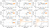 |
Fig. 4. Similar to Fig. 3, but showing RV measurements from a previous monitoring campaign (F03) and the three previous RV measurements of SMC AB12 from Foellmi (2004). These measurements have been shifted by the previously measured average RV for each star. The center and right plots on the bottom row are cumulative probability distributions. |
AB 9 has been classified as a binary candidate by F03, whose measurements indicated a value of ΔRV = 155 km/s for this source. These authors deemed it to be “marginally a binary from the RV point of view”. Their tentative orbital solution has Porb = 37.6 d and RV amplitude of K = 43 km/s. Here we find that the RV of SMC AB9 is much more constant (ΔRV = 15 km/s). This means that SMC AB9 was most likely a spurious detection in F03, as these authors already suspected. We note that when we use the He II 4686 Å line for our RV measurements of this source, we find ΔRV = 53 km/s, making it likely that the LPV (Fullerton et al. 1996; Dsilva et al. 2022) is at least partially responsible for the marginal detection in F03.
The median standard deviation of the RV measurements for individual WR stars is shown in the bottom right panel of Fig. 4. In the campaign of F03, the median σRV = 30 km/s lies somewhat above the 20 km/s that they quote as typical error for their measurements. Our campaign has a much lower median σRV ≈ 5 km/s, in line with the ΔRV result. This σRV ≈ 5 km/s is, however, larger than the statistical errors obtained from the fits to the CCFs, which are only on the order of 1 km/s. The true error is most likely larger than that, for example because of LPV.
In summary, we measure nearly constant RV values, which strongly reduces the possible binary parameter space for potential binary companions. Still, we find some RV variability that could not be explained by the statistical errors alone. Below we explore two possibilities: that the small RV variability arises from LPV (Sect. 4), and that our target stars are in binaries with low-mass and/or far-away companions (Sect. 5).
4. Line profile variability
Here we take a more detailed look at spectrum 4 of SMC AB1, taken on observation night 4, from which we infer an apparent antiphase RV motion between the N V lines and the He II absorption lines (Fig. 3). Figure 5 shows that LPV does take place in SMC AB1: compared to the co-added spectrum, spectrum 4 exhibits a higher flux at the red side (i.e., at longer wavelengths) of the N V and He II features. This excess of red flux causes an apparent shift to the red for the emission features (left panels of Fig. 5), which led us to measure positive values for their relative RVs. Conversely, the red excess causes an apparent shift to the blue for absorption features (right panels of Fig. 5), and therefore we measured negative relative RVs for them.
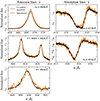 |
Fig. 5. Normalized cutouts of the co-added VLT-UVES spectrum of SMC AB1 (black lines). We also show the spectrum taken on observing night 4 (orange lines), corrected for barycentric motion. |
For the blue side of the N V emission features and the He II absorption features in spectrum 4, there seems to be no systematic shift compared to the co-added spectrum, which would be expected for RV offsets caused by binary motion. We conclude that LPV rather than binary motion is the most plausible explanation for the measured RV shifts in spectrum 4 of SMC AB1, and for the apparent antiphase motion between absorption and emission lines.
This absorption–emission antiphase motion is not as clearly seen in all of the other spectra that we have taken. This could be explained by smaller variability, as we measured relatively large RV shifts in spectrum 4 of SMC AB1. Furthermore, in SMC AB4 the He II 4339 Å and He II 4542 Å lines are in emission rather than in absorption, which may explain why the RV shifts measured with the He II and N V lines tend to be in the same direction for individual spectra of this star (Fig. 3).
A value of σRV ≈ 5 km/s caused by LPV would be the same as what was found by Dsilva et al. (2022). These authors studied LPV from N V lines by taking over 20 spectra in a narrow time interval of the wide binary star WR 138 in the Milky Way, which is an early-type WN star, like our target stars. We note that even larger RV variations (measured with a N V line in spectra of WR 6 in the Milky Way, a WN4 star) have been attributed to LPV caused by a corotating interaction region – rather than binary motion – by Barclay et al. (2024).
5. Possible presence of undetected companions
5.1. Sensitivity of our campaign to binary motion
In order explore the allowed binary parameter space for companion stars, we follow a procedure similar to the one described in Dsilva et al. (2020, 2022), and Shenar et al. (2023a). We summarize the taken procedure below. We assume that our targeted WR stars have a mass of 20 M⊙ (Hainich et al. 2015; Schootemeijer & Langer 2018). We explore orbital periods in the range of log(Porb/d) = [0, 0.1, …, 3.5] and companion masses in the range of Mcomp = [1, 2, …, 40] M⊙ (see Fig. 6). For each of the 1440 combinations of orbital period and companion mass, we simulate our observing campaign 10 000 times, by drawing a random orientation of the orbital plane (i.e., a random cos i, where i is the inclination angle to the line of sight) and a random orbital phase for the first observation. Then we measure the RV of the WR star in this mock binary at the same dates as in our observing campaign. We set the mock RV measurement error σRV, mock to zero. This is a conservative assumption, since we find that setting σRV, mock > 0 increases, on average, the mock ΔRV values. Then, for each companion mass and orbital period combination, we counted how often mock binary motion would result in a ΔRV value larger than what is observed for the WR star.
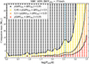 |
Fig. 6. Color-coded probability, p(ΔRVsim > ΔRVobs), that binary-induced motion would lead to a RV variation exceeding the observed ΔRVobs in SMC AB9, for different combinations of orbital period, Porb, and companion mass (see the main text for details). The higher this probability is, the less likely the source is an undetected binary. The dashed blue vertical line indicates Porb = 1 yr. |
The results for SMC AB9 (ΔRVobs = 15 km/s) are shown in Fig. 6. This figure shows that we would have most likely measured higher ΔRV values than observed if SMC AB9 had a binary companion. For companion masses above 5 M⊙ and orbital periods below one year, this probability exceeds 95% in 98,6% of the parameter space.
We can obtain an overall probability  that binarity would have been detected by our measurements when we specify underlying orbital period and mass ratio probability distributions. For flat distributions of log(Porb/d) and mass ratio, this overall probability is just the average of the probability values displayed in Fig. 6, which becomes
  . However, binary evolution models predict that in a scenario where the WR star formed through binary stripping, configurations with very low-mass companions, as well as very short or very long orbital periods, are avoided. When using underlying orbital period and mass ratio distributions motivated by binary population synthesis models (Renzo et al. 2019; Langer et al. 2020, see Appendix B.2 for details) we find even higher values of
  , while when we truncate these distributions for Porb > 30 d – since those systems have already been detected – we still find
  for SMC AB9.
For our other target stars we obtain similar results (Figs. B.4–B.9; Table B.1). Hence, for each individual WR star we can rule out most of the realistic parameter space for binaries that may have previously interacted, in particular where Porb < 1 yr. We discuss binaries with 1 yr < Porb < 10 yr in Sect. 5.2. Performing the same experiment with the F03 data reveals the possibility that companions of some tens of solar masses with Porb ≈ 1 yr could have been missed (Figs. B.10–B.16; Table B.3).
We also computed the most likely companion mass of our WR stars under the assumption that, apart from the small σCCF ≈ 1 km/s, the measured RV variability is caused by binary motion. Figure B.3 shows that for SMC AB9, this is about 1 − 3 M⊙ for periods of up to one year, increasing to beyond 5 M⊙ for periods longer than 3 yr. The most likely companion masses reside very close to the 0.5 probability contour in Fig. 6.
To construct Fig. 6 we assumed circular orbits, since we expect that if binary interaction has taken place, this would have circularized the orbit (Eq. (20) of Iorio et al. 2023). As a test, we repeated the simulations described in this section with a flat eccentricity distribution in the range 0 ≤ e ≤ 0.9. This led to detection probabilities that were smaller, but only slightly so (Table B.2 and Fig. B.1), and therefore do not change the interpretation of our results.
For all the considered ranges of the possible binary parameter space described in Appendix B, we find the lowest values for  when excluding orbital periods below 30 d and including eccentric orbits (Table B.2). For the seven target WR stars, we then find an average of
  . This implies a chance that we missed a binary companion for all of our target WR stars on the order of (1 − 0.801)7 ≈ 10−5 even for this set of assumptions.
5.2. Long-period binaries
In the last section we have seen that our small observed ΔRV values make it unlikely that our target stars have binary companions, especially with orbital periods of a year or less. Because we observed during three successive semesters, it could be more likely that we missed binary companions with an orbital period on the order of a few years in our campaign.
Here we perform an additional experiment where we explore the likelihood that all our target WR stars are in 1−10 yr binaries. If so, we would expect to measure small RV differences for observations that are separated days or weeks apart, and larger RV differences for observations taken months or years apart. In the top panel of Fig. 7 we plot with black crosses the time between successive observations (Δtsucc) against the RV difference between them (ΔRVsucc). For our seven target stars, Fig. 7 shows a total of 42 data points for successive VLT-UVES observations, including both our observations and those from Marchenko et al. (2007). There is no significant correlation in the observational data, as we obtain a value of 0.01 ± 0.10 for the slope of the linear fit (also shown in the top panel of Fig. 7). This in line with our measured σRV ≈ 5 km/s being caused by a combination of measurement errors and LPV on timescales around one day or shorter.
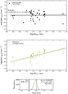 |
Fig. 7. Correlation of the time interval, Δtsucc, between two successive RV measurements and their observed ΔRVsucc. Top: The black crosses represent measurements taken in this work and in Marchenko et al. (2007). Middle: Measurements of a simulated population of long-period binaries with orbital periods between 1 and 10 years (see the main text for details), shown as colored dots. For clarity, we show only 2 of the 100 000 simulated observing campaigns. Bottom: Histogram of the 100 000 fitted slopes. The two vertical lines indicate the values of the two examples shown in the middle panel. |
To quantify how likely it is that Δtsucc and ΔRVsucc do not show a significant positive correlation if all our target stars are in 1 − 10 yr binaries, we again simulate our observing campaign as in Sect. 5.1, but now 100 000 times, for all seven target stars. We draw a random logarithm of the orbital period in the range 0 ≤ log(Porb/yr)≤1 and a random mass ratio in the range 0.05 ≤ Mcomp/MWR ≤ 2 (i.e., a companion mass in the range 1 − 40 M⊙), both from flat distributions (Öpik 1924; Kouwenhoven et al. 2007). We add a Gaussian error to each mock binary measurement, based on the observed σCCF. The green and orange dots in the middle panel of Fig. 7 show the results for two individual simulated observing campaigns; the other 99 998 are omitted for visibility purposes. We find that in all except 13 simulations (99.987%), the linear fit of Δtsucc and ΔRVsucc is larger than the observed value of 0.01 (bottom panel of Fig. 7). Therefore, it is highly unlikely that all our target stars are long-period binaries with of Porb = 1 − 10 yr.
5.3. Neutron star companions
Neutron stars (NSs) have masses in the range 1−2 M⊙, and hence we could only detect them as companions to our target WR stars if they had orbital periods of ∼30 days or less (Fig. 6). However, NSs are expected to emit X-rays arising from the accretion of material from the wind of the WR stars. F03 found upper limits of LX < 1 − 2 × 1033 erg/s based on ROSAT data. Using Eq. (1) from Shapiro & Lightman (1976) for the NS accretion radii and the stellar parameters from Hainich et al. (2015), and adopting Bondi-Hoyle accretion, we find that these X-ray non-detections exclude the presence of NSs with orbital periods of Porb ≲ 100 d. However, the accretion rates, and thus the X-ray flux, could be significantly smaller if the magnetosphere of the rotating NS star would expel a fraction of the inflowing wind material.
Independent of this, it appears unlikely that all the apparently single WR stars have NS companions, for three reasons. First, the observed WR stars in the SMC are thought to originate from main-sequence stars with M ≳ 40 M⊙ (Schootemeijer & Langer 2018; Shenar et al. 2020). Any more evolved companion, for example a compact star, would have an initial mass similar to that or higher, and therefore would most likely be a BH and not an NS (Schneider et al. 2023). Second, the majority of NS producing binaries are expected to break up when the corresponding supernova occurs (Eldridge et al. 2011; Renzo et al. 2019), which makes it unlikely that the number of WR+NS binaries is comparable to the number of WR+O star progenitors (of which there are five in the SMC; Shenar et al. 2016). Third, binary interaction in massive non-disrupted systems with NS companions has been claimed to always lead to a merger, explaining the absence of detected WR+NS binaries (van den Heuvel et al. 2017; Toalá et al. 2018). Consequently, it appears unlikely for each of our WR stars to have an NS companion, and we dismiss the possibility that all our target WR stars have NS companions.
6. Other signatures of binarity
6.1. Photometric variability
We analyzed photometric data that has become available in the last 20 years. F03 have investigated time-series photometry data of all of the SMC WR stars but SMC AB12 and the eclipsing binary SMC AB5 (Moffat et al. 1998). They found no periodic signals except for the apparently single star SMC AB4, for which they reported a 3.2σ detection of a 6.55 d period variability. This detection was for MACHO-B data (Alcock et al. 1999) but there were non-detections for MACHO-R and OGLE I data (Udalski et al. 1998).
Using the LIGHTKURVE python package (Lightkurve Collaboration 2018), we analyze OGLE III (Udalski et al. 2008) and OGLE IV (Udalski et al. 2015) time-series photometry data of all seven of our targets stars (A. Udalski, private communication). These data cover a time span of about twenty years. With the Lomb-Scargle method we obtain the power spectrum for each target WR star, exploring 106 equidistant frequencies in the range 0.001 d−1 < f < 0.67 d−1. Then we used the flatten function to calculate the S/N spectrum. We provide an overview of the OGLE data and the highest S/N values calculated from them in Table A.8. Nowhere in the considered frequency range did any of our target stars approach a threshold S/N of 4.6 (Bowman & Michielsen 2021) for periodic variability. We also provide the power spectra and phase-folded light curves in Fig. A.1, which further support the absence of convincing binary-induced signals. We are thus not able to find a significant periodic signal for any of our target stars, including SMC AB4.
6.2. Imprints of companions in the spectra
SMC AB1, 9, 10, 11, and 12 are hot objects (T* ≥ 80 kK; Hainich et al. 2015), and therefore potential cooler companions could be found by their imprints in the spectra. For example, we look for the He I 4471 Å line, which appears in stars later than O5 (Walborn et al. 2000). None of the hot WR stars in our sample show any sign of this He I line (also not after re-binning). This might be unsurprising since even in the composite spectra of the five binary SMC WR stars (which have O-star companions of tens of solar masses; see Shenar et al. 2016) the He I 4471 Å absorption line does not go deeper than 0.02 − 0.1 times the continuum. For the presence of lower-mass (and thus dimmer) stars, our RV measurements can be expected to place much stronger constraints than line strength measurements.
Other lines that we attempt to find in search for companions of hot WR stars are He I 4387 Å, He I 4713 Å, He I 4922 Å, Si IV 4089 Å, Si IV 4116 Å, and O II 4350 Å. We note that these tend to be weaker than the He I 4471 Å line in the spectra of WR binaries in the Magellanic Clouds (Shenar et al. 2016, 2019). We do not see a signature of any of these lines in the spectra of the hot WR stars that we targeted. We conclude that we are unable to find imprints of companion stars in the WR spectra, in line with the results from our RV measurements.
Finally, we inspect spectra of SMC AB2 and SMC AB4 from the Ultraviolet Legacy Library of Young Stars as Essential Standards (ULLYSES; Roman-Duval et al. 2020). We notice that for both stars, the C IV feature around 1550 Å is saturated, which is indicative of an absence of another hot star (because another hot star with a weaker wind than the WR star could contribute to the flux in this line region). The only other SMC WR star in the ULYSSES sample is SMC AB9, which is much hotter than SMC AB2 and SMC AB4 and lacks a strong C IV feature.
6.3. Absolute radial velocities and proper motions
So far we have found little evidence indicating that our target WR stars are currently in binary systems. In principle, they may have been in binary systems in the past that have broken up or merged (see also Sect. 7.1). If they were in binary systems that have been disrupted by supernova explosions, this will result in higher space velocities. To test this, we investigate their absolute RVs and proper motions.
The absolute RVs are obtained from cross-correlating our co-added spectra (Sect. 2.2) with the best-fit model atmosphere spectra from Hainich et al. (2015). Based on where the best fit of this model to the observations is achieved, we select three line regions for the cross-correlation. Two of these are the He II 4339 Å and He II 4686 Å lines. As the third line region we select N IV 4058Å for the two coldest objects (SMC AB 2 and SMC AB4), and N V 4944 Å for the other five WR stars. We define our measured absolute RV as the average measured RV and the error as the standard deviation of the three measurements (again with 1.5 degree of freedom subtracted in the divisor). We correct the co-added spectra for barycentric motion by subtracting the average barycentric velocity, which we obtain with the baryCorr function of the python package PYASL. (Piskunov & Valenti 2002) The results are shown in Table 2. We then compare the absolute RVs of our WR stars to those from stars in their vicinity. For this comparison, from the Gaia archive2 we download all DR3 sources (Gaia Collaboration 2023) that have measured RVs and reside within 15′ of our target WR stars. We exclude sources with a parallax larger than five times the parallax error to remove foreground sources (Aadland et al. 2018; Schootemeijer et al. 2021). Fig. 8 shows the absolute RVs of our targeted WR stars and the nearby sources within 15′.
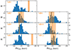 |
Fig. 8. RVs of our targeted WR stars (vertical orange lines; the shaded region indicates the error margin). The blue histograms show the RVs of Gaia DR3 sources in a 15′ radius. |
Five out of seven single WR stars have absolute RVs that are consistent with those of sources in their surroundings. For SMC AB11, its RVabs of 228 ± 8 km/s is significantly different to sources in its surroundings, where we find RVabs = 139 ± 21 km/s (the error being the standard deviation of the nearby sources’ RV, and 139 km/s being their average RV value). This makes SMC AB11 a runaway star, moving with a relative velocity of 91 ± 23 km/s in the line-of-sight direction. Similarly, for SMC AB1 we derive a relative velocity of 68 ± 35 km/s based on its RVabs = 203 ± 8 km/s, and an RVabs = 135 ± 35 km/s for sources in its vicinity. This qualifies SMC AB1 also as a runaway star.
As a check, we also look up the proper motions of SMC WR stars in Gaia DR3 and compare them to surrounding sources within 5′. We remove foreground sources as described above, and we discard sources dimmer than G = 17 or with RUWE > 1.4. We translated the proper motions intro transverse velocities, vtrans, by adopting an SMC distance of 62.44 kpc (Graczyk et al. 2020). The results are shown in Fig. 9. The transverse velocities of most of our WR stars are similar to those of their surrounding sources, except, again, for SMC AB1 and SMC AB11. We find a relative two-dimensional vtrans ≈ 107 ± 33 km/s for SMC AB11 compared to the average of the surrounding stars (the error follows from the Gaia proper motion uncertainty of SMC AB11). This confirms its nature as a runaway star. Similarly, for SMC AB1 we measure a relative vtrans = 78 km/s, in line with the result for the absolute RV.
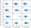 |
Fig. 9. Velocities transverse to the line of sight. Our targeted WR stars are shown in orange, and binary SMC WR stars are shown in magenta. The shown errors are obtained from proper motion errors. Gaia DR3 sources in a 5′ radius are shown in blue. |
Puzzlingly, we also find a high relative transverse velocity for SMC AB6, which is unexpected given that this is part of a multiple system (Shenar et al. 2018). This might indicate that the SMC WR proper motions are more uncertain than the errors indicate, perhaps because these very massive stars that tend to be in crowded regions. Additionally, we note that, given the errors, our method is not sensitive to intermediate-velocity runaway stars.
We take a closer look at the runaway star SMC AB11, which has a bright red source only 1″ away that we also put in the slit (Sect. 2.1). From the composite spectrum, we measure the absolute RV of the red source to see if it moves in the opposite direction of SMC AB11, which would be expected if they were in a multiple system that has been broken up. However, using the narrow Hα line we find RVabs ≈ 150 km/s, which is a very typical value in its environment (Fig. 8). This implies that the red source is a chance alignment rather than that it originates from a common multiple system with SMC AB11.
Finally, we investigate the supernova remnant (SNR) population in the SMC (Maggi et al. 2019; Matsuura et al. 2022). SMC AB11 is closest to SNR J0052−7236, which resides at a projected distance of 50 pc (3′). It has an age of about 35 kyr (Leahy & Filipović 2022). SMC AB11 would need much higher velocity of vtrans ≈ 1500 km/s to reach a 3′ separation within the lifetime of the SNR. In addition, the proper motion vector does not point back to SNR J0052−7236. Therefore, we cannot associate SMC AB11 with an SNR. We conclude the same for SMC AB1, which is not close to any known SNR in the SMC. Our inability to link SMC AB1 and SMC AB11 to a “smoking gun” SNR does not rule out that they are post-supernova runaways, since the He-burning WR lifetime is about ten times longer than the oldest SNR in the SMC (which is 35 kr; Leahy & Filipović 2022). We discuss the implications of the runaway nature of SMC AB1 and SMC AB11 further in Sect. 7.1.
7. Discussion
Schootemeijer & Langer (2018) found a fundamental difference in the internal constitution between binary and apparently single WR stars in the SMC. The binary WR stars showed a shallow internal radial H/He gradient as expected from a retreating convective core during central hydrogen burning, whereas the apparently single WR stars were shown to have an up to 10-times steeper H/He gradient, and a correspondingly less massive H-rich envelope. The shallow gradient of the WR stars in binaries is well reproduced by the mass transferring short period binary evolution models of Pauli et al. (2022). However, the steep H/He gradients require another WR star formation history.
The formation of a steep H/He gradient requires that the region with the naturally shallow gradient be mixed. As discussed by Schootemeijer & Langer (2018), this can occur either by allowing the WR progenitor to expand during its post-main-sequence evolution, such that convection induced by either hydrogen shell burning or by a convective envelope mixes the corresponding layers, or by increasing the convective core in a hydrogen-burning mass gainer. In both cases, the WR star might have lost its envelope by binary mass transfer or, as a single star, by winds or eruptions. Below, we discuss the scenarios proposed in the literature that allow for the formation of single WR stars.
7.1. Formation channel of single WR stars in the SMC
Chemically homogeneous evolution (CHE). In CHE models, rotationally induced mixing brings hydrogen-depleted material to the surface of exceptionally rapidly spinning stars (e.g., Maeder 1987; Brott et al. 2011). This scenario works most efficiently at low metallicities (Yoon et al. 2006). As such, CHE could in principle explain the presence of hydrogen-poor WR stars in the SMC (Martins et al. 2009; Hainich et al. 2015; Ramachandran et al. 2019, and see Koenigsberger et al. 2014 for SMC AB5). However, five out of seven of the single WR stars (SMC AB1, 9, 10, 11, and 12) are too hot to be explained by core hydrogen burning models (Schootemeijer & Langer 2018, their Fig. 2), but have, at the same time, a high surface hydrogen mass fraction (0.36 on average; Hainich et al. 2015). Their chemical structure is thus very inhomogeneous. In addition, the apparently single SMC WR stars show low projected rotational velocities (Martins et al. 2009; Hainich et al. 2015; Vink & Harries 2017).
Stellar mergers. We expect that mergers involving H-rich stars do not produce merger products resembling the observed single SMC WR stars, as these typically contain less than a solar mass of hydrogen (Schootemeijer & Langer 2018). In principle it is possible to produce a H-poor merger product when both stars develop He cores and then interact. Such an evolutionary path has been produced for the 2 M⊙ quasi-WR star HD 45166 (Shenar et al. 2023b). However, at high stellar masses (where stars do not develop degenerate He cores, meaning that companions have little time to catch up in their evolution) this might require a fine-tuning of the initial mass ratio and physics assumptions (Pols 1994; Wellstein & Langer 1999). Also, if mergers of two H-poor stars produced all single SMC WR stars, we would expect that in the WR+MS systems, which are their progenitors, the MS stars are close to the end of their H-burning lifetime or close to filling their Roche lobes. However, typically the MS companions are early O stars that are far from filling their Roche lobes (Shenar et al. 2016), which are not expected to exhaust H in their cores or otherwise instigate interaction before the end of the life of their companion. We are therefore unaware of a merger channel that is likely to produce seven out of twelve SMC WR stars.
Binary stripping. At first glace it seems that binary companions have not stripped our seven targeted SMC WR stars, because it is unlikely that we missed them (Sect. 5). While it is possible that we missed some rather low mass companion in a wide orbit, it is implausible that such a star could have removed the hydrogen envelope of a WR star in the past. As the progenitors of our WR stars were more massive than ∼40 M⊙ (Sect. 5.3), their binaries with companion masses below ∼5 M⊙ would have such an extreme initial mass ratio that stable mass transfer is not expected (Henneco et al. 2024). Unstable mass transfer in a system with such a mass ratio is predicted to result in a merger (Kruckow et al. 2016).
It is, in principle, possible that a WR star is stripped by a binary companion that has since exploded as a supernova, which disrupted the binary system. However, as discussed for the merger scenario above, this requires one binary component to end hydrogen burning before the other reaches core collapse. This is unlikely to happen in most of the initial binary parameter space. Still, binary stripping might be a minority channel (see also the cases of SMC AB1 and SMC AB11 presented in Sect. 6.3).
Recently, Pauli et al. (2023) explained an apparent bimodality in the temperatures of SMC WR stars by proposing that the colder WR stars SMC AB 2 and 4 are accretors in binary systems. This is in contrast to the lack of detected RV variability in our study.
Single star mass loss. Evolutionary models with SMC or near-SMC metallicity tend to use wind mass loss recipes in which winds are too weak to strip stars with initial masses around 40 M⊙ (e.g., Brott et al. 2011; Georgy et al. 2013; Choi et al. 2016; Limongi & Chieffi 2018; Schootemeijer et al. 2019). Could the mass loss rates have been underestimated in these models? For MS stars, the models typically use the Vink et al. (2001) recipe, and there is increasing evidence that it overestimates rather than underestimates MS mass loss (by a factor of ∼3; Björklund et al. 2021; Brands et al. 2022). It is perhaps more likely that stars lose a significant amount of mass as cool stars after their core-hydrogen burning phase.
One possibility for post-main-sequence self-stripping is eruptive mass loss in luminous blue variable (LBV) stars. The LBV phenomenon might be related to stars reaching the Eddington limit (Gräfener et al. 2012; Sanyal et al. 2017). According to recent predictions, this can happen in evolved SMC stars with initial masses as low as 30 M⊙ and lead to eruptive mass loss that can strip their H-rich envelope (Cheng et al. 2024). This seems to be consistent with the initial masses of M ≳ 30 − 40 M⊙ for SMC WR stars (Table 3). The SMC harbors two stars that show or have shown LBV behavior (see Richardson & Mehner 2018, also for two more candidates). One of these (HD 5980) underwent an LBV outburst in the 1990s and at present manifests itself as a WR star in the only WR+WR binary in the SMC (Koenigsberger et al. 2010). The other is R 40 (Szeifert et al. 1993; Agliozzo et al. 2021), which is currently in an LBV eruption episode, and it has an uncertain but seemingly high mass loss rate of 10−4 − 10−3 M⊙/yr (Campagnolo et al. 2018). Both sources imply that LBV mass loss could play a role in the production of WR stars at low metallicity. An SMC population of two LBVs and on the order of ten wind-stripped WR stars would be in line with the Large Magellanic Cloud (LMC) and Milky Way, where LBVs are also rarer than WR stars by a factor of at least a few (Richardson & Mehner 2018; van der Hucht 2001; Shenar et al. 2019). A caveat might be that LBVs in the LMC seem to be much more isolated than O and WN (although not WC) stars, which could indicate that (at least in the LMC) LBVs could be accretors in binary systems (Smith & Tombleson 2015).
Initial masses and He core masses found for the SMC WR stars.
Wind mass loss during a red supergiant (RSG) phase could also be responsible for stripping the outer layers of our WR progenitors. Mass loss rates of RSGs are notoriously uncertain and also their metallicity dependence is not established. Therefore, RSG mass loss rates in the SMC could occupy a wide range of values (see, e.g., Fig. 15 of Yang et al. 2023). Some mass loss rate predictions shown there increase steeply with luminosity and reach values at log(L/L⊙)≈5.5 that are high enough to strip H-rich envelopes of massive stars on timescales of ∼10 kyr (Beasor et al. 2023; Yang et al. 2023). However, these mass-loss rates at the bright end are the most uncertain, where RSGs are scarce. Related to this, we note that Kee et al. (2021) found that high and metallicity-independent mass loss rates can be achieved if turbulent velocities in RSGs are high.
Resumé. From the discussion above, we conclude that CHE, stellar mergers, and binary stripping are unlikely to constitute the dominant channel for producing single WR stars in the SMC. It follows that single star mass loss – most probably in the LBV or RSG phase – is likely responsible for the loss of the H-rich envelope in the majority of the investigated SMC WR stars.
7.2. Implications for the outcome of massive binary interactions at low metallicities
After showing that binary evolution was likely not important for the majority of the seven targeted SMC WR stars, let us assume that the detected binaries constitute the whole SMC WR binary population. All five binaries have short orbital periods in the range 6 d < Porb < 20 d. We use initial-final orbital separation relations (Soberman et al. 1997; Tauris & van den Heuvel 2006) to find possible solutions for the initial orbital periods for SMC AB6, 7, and 8 (SMC AB3 has a poorly defined mass ratio, and the initial-final separation formula likely does not apply to the evolutionary history of SMC AB5; see Koenigsberger et al. 2014; Schootemeijer & Langer 2018). Under the assumption that mass stripped away from the donor either ends up on the accretor or is lost from the accretor, there are no solutions for Porb, ini > 25 d, regardless of the adopted mass transfer efficiency. Even though this is low-number statistics, the apparent absence of medium- to long-period binaries in the SMC WR population appears striking. It could imply that massive longer-period binaries at low metallicity merge upon binary interaction. This might impede the channel for producing binary BH mergers from isolated binary evolution, which often involves stars with large initial periods (Belczynski et al. 2016; Kruckow et al. 2018). Therefore, this needs to be carefully checked in future work.
Interestingly, there are also no known binaries with Porb ≥ 40 d among the “classical” WR stars on the nitrogen sequence (subtype earlier than WN5) in the LMC (Foellmi et al. 2003b; Shenar et al. 2019). Since there are over ten times more WN stars in the LMC than in the SMC, this seems to exacerbate the lack of long- and intermediate period WR binaries at low metallicity. However, the LMC WR stars have not been monitored with high-quality observations such as those presented in this study. The LMC would thus be a good place to further investigate this issue.
Additionally, all SMC WR stars in binaries have companions that are of similar or higher mass than the WR star (with mass ratios between 1 and 3; F03, Shenar et al. 2016). This may require a non-negligible mass transfer efficiency in the systems that survived binary interaction.
7.3. Implications for BH masses at low metallicities
Our finding that the majority of the apparently single SMC WR stars lost their envelope without the help of a binary companion has direct consequences for the BH population produced by the massive stars in the SMC. It makes these stars uniquely suitable to investigate the initial mass – final mass (Mini − Mfinal) relation because of two properties: (i) they have H-rich layers near their surfaces, but these contain only ∼1 M⊙ of material (Schootemeijer & Langer 2018), and (ii) they have low mass loss rates (at which they lose M ≲ 1 M⊙ during their WR lifetime; Hainich et al. 2015). This implies that their current mass, their He core mass, and their final mass Mfinal are practically the same3. We used this property to obtain the Mini − Mfinal relation of the single SMC WR stars.
First, we obtained the He core masses of the SMC WR stars from the best-fit models of Schootemeijer & Langer (2018), from their large grid of synthetic massive star models with predefined He core masses, surface hydrogen abundances, and H/He gradients. We then used the initial mass–He core mass relations from stellar evolution models (Schootemeijer et al. 2019, with an overshooting value of 0.33) to obtain Mini − Mfinal relations. To estimate the errors, we assumed that the uncertainty in luminosity (from Hainich et al. 2015; Shenar et al. 2016, 2018) propagates into the uncertainty in mass. The error on the mass then depends on the slope of the mass–luminosity relation, which we obtained from Gräfener et al. (2011). We repeated the analysis based on the observational WR star properties obtained by Martins et al. (2009), Martins (2023), who found somewhat lower luminosities.
The results define the empirical initial-final mass relation shown as the thick gray line in Fig. 10, whose width reflects the error in this relation (see also Table 3). It is well defined in the initial mass range 40 − 65 M⊙ (or 30 − 50 M⊙ based on the luminosities of Martins et al.), and extrapolated to ∼100 M⊙.
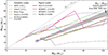 |
Fig. 10. Initial mass–final mass relations for SMC stars. Data points of SMC WR stars are shown with circles (based on Hainich et al. 2015) and squares (based on Martins et al. 2009; Martins 2023), the numbers indicating their identifier (e.g., 1 for SMC AB1). The gray shaded region indicates He core masses at the terminal-age main sequence (MHe core, TAMS) from evolutionary models of Schootemeijer et al. (2019), for overshooting values between 0.22 and 0.44. The colored lines show the following relations from literature: MIST (Dotter 2016; Choi et al. 2016), Schn23 (Schneider et al. 2023), Bonn (Schootemeijer et al. 2019), Geneva (Georgy et al. 2013), SEVN+PARSEC (Iorio et al. 2023, overshooting value of 0.4), Belc10 (Belczynski et al. 2010, data taken from Fig. 2 of Banerjee et al. 2020), MOBSE (Giacobbo et al. 2018), and Hurl00 (Hurley et al. 2000, data taken from Fig. 1 of Belczynski et al. 2010). |
In Fig. 10, we compare our result with initial-final mass relation or initial mass–BH mass relations obtained from detailed stellar evolution calculations, or used in so-called rapid binary evolution models. To obtain data from works from the literature that provide no online data apart from their plots, we used Engauge Digitizer again. Belczynski et al. (2010), Banerjee et al. (2020), and Giacobbo et al. (2018) provide remnant masses rather than final stellar masses – for these, to obtain the final masses we divide the remnant masses by 0.90, as these studies assumed that the gravitational BH mass is 10% smaller than the baryonic mass. We only show the mass range Mini > 32 M⊙, since for lower masses, where the CO core mass is lower than 11 M⊙, these codes assume BH fallback fractions lower than unity (Fryer et al. 2012). The Mini − Mfinal relations from the literature roughly come in two flavors: those that experience strong LBV mass loss in the mass range 40 < Mini/M⊙ < 80, and those that do not.
7.3.1. Initial–final mass relations with strong LBV mass loss
The mass-loss prescription from Belczynski et al. (2010) includes a strong, metallicity-independent LBV mass loss rate of 1.5 × 10⁻⁴ M⊙/yr, which in practice removes all the hydrogen-rich layers of stars born more massive than 40 M⊙. It is widely used to predict BH–BH merger rates in rapid binary evolution codes (e.g., COMPAS; Riley et al. 2022). It is also used in a non-default simulation of MOBSE (MOBSE2; Giacobbo et al. 2018) and the triple evolution code TRES (Toonen et al. 2016; Kummer et al. 2023). Also, many N-body simulations of dynamical BH-BH binary formation include the prescription of Belczynski et al. (2010) for example simulations of young star clusters (Chattopadhyay et al. 2022; Fragione et al. 2022a), which include NBODY7 (Banerjee et al. 2020; Banerjee 2021) and PeTar (Wang et al. 2020; Barber et al. 2024), as well as simulations around galactic nuclei (Antonini & Rasio 2016; Tagawa et al. 2020; Fragione et al. 2022b) and simulations of globular clusters (Rodriguez et al. 2016; Antonini & Gieles 2020). The high amount of late-phase mass loss in these simulations seems to be in agreement with our findings at SMC metallicity. However, we find (while assuming negligible WR mass loss) somewhat higher final masses than what is predicted by Belczynski et al. (2010), most likely because of their high WR mass loss rates, which are about five times larger than those that are observed for single SMC WR stars (Hainich et al. 2015).
The mass loss prescription of Hurley et al. (2000) includes, apart from strong LBV mass loss, metallicity-independent WR winds. These overestimate the mass loss rates of SMC WR stars by about a factor of 20 compared to what is observed by Hainich et al. (2015), and lead to very low final masses. The Hurley et al. (2000) prescription is used in BH–BH merger simulations of globular clusters (Askar et al. 2017; Hong et al. 2018; Samsing et al. 2018) and star clusters near galactic nuclei (Petrovich & Antonini 2017).
7.3.2. Initial–final mass relations with weak LBV mass loss
Many codes use or obtain Mini − Mfinal relations under the assumption of less drastic late-phase mass loss near SMC metallicity, which leads to higher final masses than we infer for SMC WR stars. Examples are SEVN+PARSEC (Spera et al. 2015; Iorio et al. 2023), which uses PARSEC models (Tang et al. 2014; Chen et al. 2015), the single-star models of Schneider et al. (2023), MIST (Dotter 2016; Choi et al. 2016), Geneva models (Georgy et al. 2013), and Bonn models (here showing Schootemeijer et al. 2019, which uses the same mass-loss recipe as Brott et al. 2011 and ComBinE; Kruckow et al. 2018). Moreover, in the latest prescription of MOBSE (Giacobbo et al. 2018) called MOBSE1, the LBV mass loss prescription is Z-dependent for stars with initial masses up to ∼80 M⊙ (i.e., up to the point where stars approach the Eddington limit, following Tang et al. 2014; Chen et al. 2015). This allows 40−80 M⊙ models near SMC metallicity to retain more H-rich layers and produce much more massive BHs than with the prescription of Belczynski et al. (2010). The MOBSE1 prescription is used in other rapid binary evolution codes (e.g., COSMIC; Breivik et al. 2020) and N-body simulations of young star clusters (Di Carlo et al. 2019; Santoliquido et al. 2020; Rastello et al. 2021; Torniamenti et al. 2022), nuclear star clusters (Stephan et al. 2019; Wang et al. 2021), and globular clusters (Mapelli et al. 2021). Our results imply that the mass loss rates used in these calculations are mostly too low.
7.3.3. Implications for population synthesis of double BH merger progenitors
Our results indicate that Mini − Mfinal relations that include strong late-phase mass loss (e.g., Belczynski et al. 2010) are preferable at ZSMC. Relations calculated without strong late-phase mass loss around SMC metallicity in the initial mass range of 40 M⊙ to 80 M⊙ (e.g., MOBSE1 and SEVN+PARSEC) seem to overestimate final masses of single stars. This result might be of particular importance for simulations of double BH mergers produced via the dynamical channel, since there stars that lived as single stars can be involved in double BH mergers.
For double BH merger progenitors produced by isolated binary evolution, the inferred strong late-phase mass loss might only be of importance if it is LBV rather than RSG mass loss that sheds the envelope. Unlike strong RSG mass loss, strong LBV mass loss might prevent very massive stars from expanding to large radii, and thereby prevent a common-envelope phase that tightens the BH–BH progenitor system. Our study cannot identify which of the two channels (LBV or RSG mass loss) is favorable.
8. Conclusions
We used high-quality spectra taken with VLT-UVES during three consecutive semesters to monitor the RVs of all seven apparently single known SMC WR stars, in search of binary reflex motion. To measure the RVs, we used narrow N V lines, which turned out to be remarkably stable. We find σRV values of ∼5 km/s, and all seven WR stars have ΔRV values in the range 6 km/s to 23 km/s, including the former binary candidate WR star SMC AB9. We argue that LPV from atmospheric or wind variability can account for these small RV variations.
For individual stars, our Monte Carlo simulations rule out the presence of companions more massive than 5 M⊙ and orbital periods shorter than one year with at least ∼95% confidence. Statistically, this makes it practically impossible that we missed such companions for all of them. Companions with lower masses are thought to merge with their primary star rather than strip its envelope. When considering underlying orbital period distributions of up to ten years, we still estimate a probability below ∼10−5 that all our seven target SMC WR stars are binaries. Based on a lack of correlation of ΔRV measurements between successive exposures and the time elapsed between them, we can further rule out that all of our target stars are in long-period binaries (1 − 10 yr). Moreover, our simulations show that previous studies were not sensitive to a large part of the binary parameter space. The fraction of known SMC WR stars with detected binary companions remains at 0.42.
SMC AB1 and SMC AB11 appear to be runaway stars with relative line-of-sight velocities of ∼80 km/s compared to their surroundings. The proper motions of these sources strengthen this finding. While such high velocities are not preferred in population synthesis models, Eldridge et al. (2011) predict runaway WR stars with space velocities of up to 120 km/s. Furthermore, Evans et al. (2011) and Sana et al. (2022) find runaway O stars with masses of up to ∼90 M⊙ in the LMC with similarly high runaway velocities.
Our results imply that for SMC stars above ∼40 M⊙, single stars lose the majority of their hydrogen-rich envelope, and that a binary companion is not required for this. We argue that late-phase mass loss in the LBV or RSG phase is most likely the mechanism responsible for stripping these stars so they become WR stars. Our results put strong constraints on the maximum BH mass that can emerge from stars more massive than ∼40 M⊙.
All five of the known binary WR stars in the SMC show orbital periods below 20 d. Although their number is small, this could imply that massive interacting long-period binaries at low metallicities merge. While more work is needed to substantiate this hypothesis, it would suggest that the predictions for the double BH merger rate based on isolated evolution of long-period binaries are largely overestimated.
SMC AB2 and SMC AB4 are relatively cold objects that could also burn H in their cores (Schootemeijer & Langer 2018). We therefore exclude them from this analysis.
Acknowledgments
We thank the anonymous referee for a constructive report and useful suggestions. We warmly thank Andrzej Udalski for sending us the OGLE-III and OGLE-IV data of our target stars. Equally warmly, we thank Rainer Hainich for providing the best-fit model atmosphere spectra. AS thanks Frank Backs, Sarah Brands, Michal Pawlak, Philipp Podsiadlowski, and Fabian Schneider for useful discussions. We thank ESO for delivering the excellent spectra that made this study possible. The research leading to these results has received funding from the European Research Council (ERC) under the European Union’s Horizon 2020 research and innovation programme (grant agreement numbers 772225: MULTIPLES).
References
- Aadland, E., Massey, P., Neugent, K. F., & Drout, M. R. 2018, AJ, 156, 294 [NASA ADS] [CrossRef] [Google Scholar]
- Abbott, B. P., Abbott, R., Abbott, T. D., et al. 2016, Phys. Rev. Lett., 116, 061102 [Google Scholar]
- Adams, N. J., Conselice, C. J., Ferreira, L., et al. 2023, MNRAS, 518, 4755 [Google Scholar]
- Agliozzo, C., Phillips, N., Mehner, A., et al. 2021, A&A, 655, A98 [NASA ADS] [CrossRef] [EDP Sciences] [Google Scholar]
- Alcock, C., Allsman, R. A., Alves, D. R., et al. 1999, PASP, 111, 1539 [NASA ADS] [CrossRef] [Google Scholar]
- Antonini, F., & Gieles, M. 2020, Phys. Rev. D, 102, 123016 [NASA ADS] [CrossRef] [Google Scholar]
- Antonini, F., & Rasio, F. A. 2016, ApJ, 831, 187 [Google Scholar]
- Askar, A., Szkudlarek, M., Gondek-Rosińska, D., Giersz, M., & Bulik, T. 2017, MNRAS, 464, L36 [CrossRef] [Google Scholar]
- Azzopardi, M., & Breysacher, J. 1979, A&A, 75, 120 [NASA ADS] [Google Scholar]
- Banerjee, S. 2021, MNRAS, 500, 3002 [Google Scholar]
- Banerjee, S., Belczynski, K., Fryer, C. L., et al. 2020, A&A, 639, A41 [NASA ADS] [CrossRef] [EDP Sciences] [Google Scholar]
- Barber, J., Chattopadhyay, D., & Antonini, F. 2024, MNRAS, 527, 7363 [Google Scholar]
- Barclay, K. D. G., Rosu, S., Richardson, N. D., et al. 2024, MNRAS, 527, 2198 [Google Scholar]
- Bartzakos, P., Moffat, A. F. J., & Niemela, V. S. 2001, MNRAS, 324, 18 [NASA ADS] [CrossRef] [Google Scholar]
- Beasor, E. R., Davies, B., Smith, N., et al. 2023, MNRAS, 524, 2460 [Google Scholar]
- Belczynski, K., Dominik, M., Bulik, T., et al. 2010, ApJ, 715, L138 [Google Scholar]
- Belczynski, K., Holz, D. E., Bulik, T., & O’Shaughnessy, R. 2016, Nature, 534, 512 [NASA ADS] [CrossRef] [Google Scholar]
- Björklund, R., Sundqvist, J. O., Puls, J., & Najarro, F. 2021, A&A, 648, A36 [EDP Sciences] [Google Scholar]
- Bowman, D. M., & Michielsen, M. 2021, A&A, 656, A158 [NASA ADS] [CrossRef] [EDP Sciences] [Google Scholar]
- Brands, S. A., de Koter, A., Bestenlehner, J. M., et al. 2022, A&A, 663, A36 [Google Scholar]
- Breivik, K., Coughlin, S., Zevin, M., et al. 2020, ApJ, 898, 71 [Google Scholar]
- Breysacher, J., & Westerlund, B. E. 1978, A&A, 67, 261 [NASA ADS] [Google Scholar]
- Brott, I., de Mink, S. E., Cantiello, M., et al. 2011, A&A, 530, A115 [NASA ADS] [CrossRef] [EDP Sciences] [Google Scholar]
- Campagnolo, J. C. N., Borges Fernandes, M., Drake, N. A., et al. 2018, A&A, 613, A33 [NASA ADS] [CrossRef] [EDP Sciences] [Google Scholar]
- Castellano, M., Fontana, A., Treu, T., et al. 2022, ApJ, 938, L15 [NASA ADS] [CrossRef] [Google Scholar]
- Chattopadhyay, D., Hurley, J., Stevenson, S., & Raidani, A. 2022, MNRAS, 513, 4527 [NASA ADS] [CrossRef] [Google Scholar]
- Chen, Y., Bressan, A., Girardi, L., et al. 2015, MNRAS, 452, 1068 [Google Scholar]
- Cheng, S. J., Goldberg, J. A., Cantiello, M., et al. 2024, ArXiv e-prints [arXiv:2405.12274] [Google Scholar]
- Choi, J., Dotter, A., Conroy, C., et al. 2016, ApJ, 823, 102 [Google Scholar]
- Dekker, H., D’Odorico, S., Kaufer, A., Delabre, B., & Kotzlowski, H. 2000, SPIE Conf. Ser., 4008, 534 [Google Scholar]
- Di Carlo, U. N., Giacobbo, N., Mapelli, M., et al. 2019, MNRAS, 487, 2947 [NASA ADS] [CrossRef] [Google Scholar]
- Dotter, A. 2016, ApJS, 222, 8 [Google Scholar]
- Dsilva, K., Shenar, T., Sana, H., & Marchant, P. 2020, A&A, 641, A26 [NASA ADS] [CrossRef] [EDP Sciences] [Google Scholar]
- Dsilva, K., Shenar, T., Sana, H., & Marchant, P. 2022, A&A, 664, A93 [NASA ADS] [CrossRef] [EDP Sciences] [Google Scholar]
- Dsilva, K., Shenar, T., Sana, H., & Marchant, P. 2023, A&A, 674, A88 [NASA ADS] [CrossRef] [EDP Sciences] [Google Scholar]
- Eldridge, J. J., Langer, N., & Tout, C. A. 2011, MNRAS, 414, 3501 [NASA ADS] [CrossRef] [Google Scholar]
- Evans, C. J., Taylor, W. D., Hénault-Brunet, V., et al. 2011, A&A, 530, A108 [NASA ADS] [CrossRef] [EDP Sciences] [Google Scholar]
- Foellmi, C. 2004, A&A, 416, 291 [NASA ADS] [CrossRef] [EDP Sciences] [Google Scholar]
- Foellmi, C., Moffat, A. F. J., & Guerrero, M. A. 2003a, MNRAS, 338, 360 [NASA ADS] [CrossRef] [Google Scholar]
- Foellmi, C., Moffat, A. F. J., & Guerrero, M. A. 2003b, MNRAS, 338, 1025 [NASA ADS] [CrossRef] [Google Scholar]
- Fragione, G., Kocsis, B., Rasio, F. A., & Silk, J. 2022a, ApJ, 927, 231 [NASA ADS] [CrossRef] [Google Scholar]
- Fragione, G., Loeb, A., Kocsis, B., & Rasio, F. A. 2022b, ApJ, 933, 170 [NASA ADS] [CrossRef] [Google Scholar]
- Fryer, C. L., Belczynski, K., Wiktorowicz, G., et al. 2012, ApJ, 749, 91 [Google Scholar]
- Fullerton, A. W., Gies, D. R., & Bolton, C. T. 1996, ApJS, 103, 475 [NASA ADS] [CrossRef] [Google Scholar]
- Gaia Collaboration (Vallenari, A., et al.) 2023, A&A, 674, A1 [NASA ADS] [CrossRef] [EDP Sciences] [Google Scholar]
- Georgy, C., Ekström, S., Eggenberger, P., et al. 2013, A&A, 558, A103 [NASA ADS] [CrossRef] [EDP Sciences] [Google Scholar]
- Giacobbo, N., Mapelli, M., & Spera, M. 2018, MNRAS, 474, 2959 [Google Scholar]
- Graczyk, D., Pietrzyński, G., Thompson, I. B., et al. 2020, ApJ, 904, 13 [Google Scholar]
- Gräfener, G., Vink, J. S., de Koter, A., & Langer, N. 2011, A&A, 535, A56 [NASA ADS] [CrossRef] [EDP Sciences] [Google Scholar]
- Gräfener, G., Owocki, S. P., & Vink, J. S. 2012, A&A, 538, A40 [NASA ADS] [CrossRef] [EDP Sciences] [Google Scholar]
- Hainich, R., Pasemann, D., Todt, H., et al. 2015, A&A, 581, A21 [NASA ADS] [CrossRef] [EDP Sciences] [Google Scholar]
- Henneco, J., Schneider, F. R. N., & Laplace, E. 2024, A&A, 682, A169 [NASA ADS] [CrossRef] [EDP Sciences] [Google Scholar]
- Hong, J., Vesperini, E., Askar, A., et al. 2018, MNRAS, 480, 5645 [NASA ADS] [CrossRef] [Google Scholar]
- Hurley, J. R., Pols, O. R., & Tout, C. A. 2000, MNRAS, 315, 543 [Google Scholar]
- Iorio, G., Mapelli, M., Costa, G., et al. 2023, MNRAS, 524, 426 [NASA ADS] [CrossRef] [Google Scholar]
- Kee, N. D., Sundqvist, J. O., Decin, L., de Koter, A., & Sana, H. 2021, A&A, 646, A180 [NASA ADS] [CrossRef] [EDP Sciences] [Google Scholar]
- Koenigsberger, G., Georgiev, L., Hillier, D. J., et al. 2010, AJ, 139, 2600 [NASA ADS] [CrossRef] [Google Scholar]
- Koenigsberger, G., Morrell, N., Hillier, D. J., et al. 2014, AJ, 148, 62 [Google Scholar]
- Kouwenhoven, M. B. N., Brown, A. G. A., Portegies Zwart, S. F., & Kaper, L. 2007, A&A, 474, 77 [NASA ADS] [CrossRef] [EDP Sciences] [Google Scholar]
- Kruckow, M. U., Tauris, T. M., Langer, N., et al. 2016, A&A, 596, A58 [NASA ADS] [CrossRef] [EDP Sciences] [Google Scholar]
- Kruckow, M. U., Tauris, T. M., Langer, N., Kramer, M., & Izzard, R. G. 2018, MNRAS, 481, 1908 [CrossRef] [Google Scholar]
- Kummer, F., Toonen, S., & de Koter, A. 2023, A&A, 678, A60 [NASA ADS] [CrossRef] [EDP Sciences] [Google Scholar]
- Langer, N., Schürmann, C., Stoll, K., et al. 2020, A&A, 638, A39 [NASA ADS] [CrossRef] [EDP Sciences] [Google Scholar]
- Leahy, D. A., & Filipović, M. D. 2022, ApJ, 931, 20 [NASA ADS] [CrossRef] [Google Scholar]
- Lightkurve Collaboration (Cardoso, J. V. D. M., et al.) 2018, Astrophysics Source Code Library [record ascl:1812.013] [Google Scholar]
- Limongi, M., & Chieffi, A. 2018, ApJS, 237, 13 [NASA ADS] [CrossRef] [Google Scholar]
- Maeder, A. 1987, A&A, 178, 159 [NASA ADS] [Google Scholar]
- Maggi, P., Filipović, M. D., Vukotić, B., et al. 2019, A&A, 631, A127 [NASA ADS] [CrossRef] [EDP Sciences] [Google Scholar]
- Mapelli, M., Dall’Amico, M., Bouffanais, Y., et al. 2021, MNRAS, 505, 339 [CrossRef] [Google Scholar]
- Marchenko, S. V., Foellmi, C., Moffat, A. F. J., et al. 2007, ApJ, 656, L77 [NASA ADS] [CrossRef] [Google Scholar]
- Martins, F. 2023, A&A, 680, A22 [NASA ADS] [CrossRef] [EDP Sciences] [Google Scholar]
- Martins, F., Hillier, D. J., Bouret, J. C., et al. 2009, A&A, 495, 257 [NASA ADS] [CrossRef] [EDP Sciences] [Google Scholar]
- Massey, P. 2003, ARA&A, 41, 15 [NASA ADS] [CrossRef] [Google Scholar]
- Massey, P., & Duffy, A. S. 2001, ApJ, 550, 713 [NASA ADS] [CrossRef] [Google Scholar]
- Matsuura, M., Ayley, V., Chawner, H., et al. 2022, MNRAS, 513, 1154 [NASA ADS] [CrossRef] [Google Scholar]
- Mitchell, M., Muftakhidinov, B., Winchen, T., et al. 2020, https://doi.org/10.5281/zenodo.3941227 [Google Scholar]
- Moffat, A. F. J. 1982, ApJ, 257, 110 [NASA ADS] [CrossRef] [Google Scholar]
- Moffat, A. F. J. 1988, ApJ, 330, 766 [CrossRef] [Google Scholar]
- Moffat, A. F. J., Breysacher, J., & Seggewiss, W. 1985, ApJ, 292, 511 [NASA ADS] [CrossRef] [Google Scholar]
- Moffat, A. F. J., Marchenko, S. V., Bartzakos, P., et al. 1998, ApJ, 497, 896 [NASA ADS] [CrossRef] [Google Scholar]
- Morgan, D. H., Vassiliadis, E., & Dopita, M. A. 1991, MNRAS, 251, 51P [NASA ADS] [CrossRef] [Google Scholar]
- Neugent, K. F., Massey, P., & Morrell, N. 2018, ApJ, 863, 181 [NASA ADS] [CrossRef] [Google Scholar]
- Öpik, E. 1924, Publications of the Tartu Astrofizica Observatory, 25, 1 [Google Scholar]
- Pauli, D., Langer, N., Aguilera-Dena, D. R., Wang, C., & Marchant, P. 2022, A&A, 667, A58 [NASA ADS] [CrossRef] [EDP Sciences] [Google Scholar]
- Pauli, D., Oskinova, L. M., Hamann, W. R., et al. 2023, A&A, 673, A40 [NASA ADS] [CrossRef] [EDP Sciences] [Google Scholar]
- Petrovich, C., & Antonini, F. 2017, ApJ, 846, 146 [NASA ADS] [CrossRef] [Google Scholar]
- Piskunov, N. E., & Valenti, J. A. 2002, A&A, 385, 1095 [NASA ADS] [CrossRef] [EDP Sciences] [Google Scholar]
- Pols, O. R. 1994, A&A, 290, 119 [Google Scholar]
- Ramachandran, V., Hamann, W. R., Oskinova, L. M., et al. 2019, A&A, 625, A104 [NASA ADS] [CrossRef] [EDP Sciences] [Google Scholar]
- Rastello, S., Mapelli, M., Di Carlo, U. N., et al. 2021, MNRAS, 507, 3612 [CrossRef] [Google Scholar]
- Renzo, M., Zapartas, E., de Mink, S. E., et al. 2019, A&A, 624, A66 [NASA ADS] [CrossRef] [EDP Sciences] [Google Scholar]
- Richardson, N. D., & Mehner, A. 2018, Res. Notes Am. Astron. Soc., 2, 121 [Google Scholar]
- Riley, J., Agrawal, P., Barrett, J. W., et al. 2022, ApJS, 258, 34 [NASA ADS] [CrossRef] [Google Scholar]
- Rodriguez, C. L., Chatterjee, S., & Rasio, F. A. 2016, Phys. Rev. D, 93, 084029 [NASA ADS] [CrossRef] [Google Scholar]
- Roman-Duval, J., Proffitt, C. R., Taylor, J. M., et al. 2020, Res. Notes Am. Astron. Soc., 4, 205 [Google Scholar]
- Samsing, J., Askar, A., & Giersz, M. 2018, ApJ, 855, 124 [NASA ADS] [CrossRef] [Google Scholar]
- Sana, H., de Mink, S. E., de Koter, A., et al. 2012, Science, 337, 444 [Google Scholar]
- Sana, H., Ramírez-Agudelo, O. H., Hénault-Brunet, V., et al. 2022, A&A, 668, L5 [NASA ADS] [CrossRef] [EDP Sciences] [Google Scholar]
- Sanduleak, N. 1968, AJ, 73, 246 [Google Scholar]
- Sanduleak, N. 1969, AJ, 74, 877 [NASA ADS] [CrossRef] [Google Scholar]
- Santoliquido, F., Mapelli, M., Bouffanais, Y., et al. 2020, ApJ, 898, 152 [Google Scholar]
- Sanyal, D., Langer, N., Szécsi, D., Yoon, S.-C., & Grassitelli, L. 2017, A&A, 597, A71 [NASA ADS] [CrossRef] [EDP Sciences] [Google Scholar]
- Schneider, F. R. N., Podsiadlowski, P., & Laplace, E. 2023, ApJ, 950, L9 [NASA ADS] [CrossRef] [Google Scholar]
- Schootemeijer, A., & Langer, N. 2018, A&A, 611, A75 [NASA ADS] [CrossRef] [EDP Sciences] [Google Scholar]
- Schootemeijer, A., Langer, N., Grin, N. J., & Wang, C. 2019, A&A, 625, A132 [NASA ADS] [CrossRef] [EDP Sciences] [Google Scholar]
- Schootemeijer, A., Langer, N., Lennon, D., et al. 2021, A&A, 646, A106 [NASA ADS] [CrossRef] [EDP Sciences] [Google Scholar]
- Shapiro, S. L., & Lightman, A. P. 1976, ApJ, 204, 555 [NASA ADS] [CrossRef] [Google Scholar]
- Shenar, T., Hainich, R., Todt, H., et al. 2016, A&A, 591, A22 [NASA ADS] [CrossRef] [EDP Sciences] [Google Scholar]
- Shenar, T., Hainich, R., Todt, H., et al. 2018, A&A, 616, A103 [NASA ADS] [CrossRef] [EDP Sciences] [Google Scholar]
- Shenar, T., Sablowski, D. P., Hainich, R., et al. 2019, A&A, 627, A151 [NASA ADS] [CrossRef] [EDP Sciences] [Google Scholar]
- Shenar, T., Gilkis, A., Vink, J. S., Sana, H., & Sander, A. A. C. 2020, A&A, 634, A79 [NASA ADS] [CrossRef] [EDP Sciences] [Google Scholar]
- Shenar, T., Sana, H., Crowther, P. A., et al. 2023a, A&A, 679, A36 [NASA ADS] [CrossRef] [EDP Sciences] [Google Scholar]
- Shenar, T., Wade, G. A., Marchant, P., et al. 2023b, Science, 381, 761 [NASA ADS] [CrossRef] [Google Scholar]
- Smith, L. F. 1968, MNRAS, 140, 409 [NASA ADS] [Google Scholar]
- Smith, N., & Tombleson, R. 2015, MNRAS, 447, 598 [NASA ADS] [CrossRef] [Google Scholar]
- Soberman, G. E., Phinney, E. S., & van den Heuvel, E. P. J. 1997, A&A, 327, 620 [NASA ADS] [Google Scholar]
- Spera, M., Mapelli, M., & Bressan, A. 2015, MNRAS, 451, 4086 [NASA ADS] [CrossRef] [Google Scholar]
- Stephan, A. P., Naoz, S., Ghez, A. M., et al. 2019, ApJ, 878, 58 [NASA ADS] [CrossRef] [Google Scholar]
- Stoehr, F., White, R., Smith, M., et al. 2008, ASP Conf. Ser., 394, 505 [NASA ADS] [Google Scholar]
- Szécsi, D., Langer, N., Yoon, S.-C., et al. 2015, A&A, 581, A15 [NASA ADS] [CrossRef] [EDP Sciences] [Google Scholar]
- Szeifert, T., Stahl, O., Wolf, B., et al. 1993, A&A, 280, 508 [NASA ADS] [Google Scholar]
- Tagawa, H., Haiman, Z., & Kocsis, B. 2020, ApJ, 898, 25 [NASA ADS] [CrossRef] [Google Scholar]
- Tang, J., Bressan, A., Rosenfield, P., et al. 2014, MNRAS, 445, 4287 [NASA ADS] [CrossRef] [Google Scholar]
- Tauris, T. M., & van den Heuvel, E. P. J. 2006, Camb. Astrophys. Ser., 39, 623 [NASA ADS] [Google Scholar]
- Toalá, J. A., Oskinova, L. M., Hamann, W. R., et al. 2018, ApJ, 869, L11 [CrossRef] [Google Scholar]
- Toonen, S., Hamers, A., & Portegies Zwart, S. 2016, Comput. Astrophys. Cosmol., 3, 6 [NASA ADS] [CrossRef] [Google Scholar]
- Torniamenti, S., Rastello, S., Mapelli, M., et al. 2022, MNRAS, 517, 2953 [NASA ADS] [CrossRef] [Google Scholar]
- Udalski, A., Szymanski, M., Kubiak, M., et al. 1998, Acta Astron., 48, 147 [NASA ADS] [Google Scholar]
- Udalski, A., Szymanski, M. K., Soszynski, I., & Poleski, R. 2008, Acta Astron., 58, 69 [NASA ADS] [Google Scholar]
- Udalski, A., Szymański, M. K., & Szymański, G. 2015, Acta Astron., 65, 1 [NASA ADS] [Google Scholar]
- van den Heuvel, E. P. J., Portegies Zwart, S. F., & de Mink, S. E. 2017, MNRAS, 471, 4256 [Google Scholar]
- van der Hucht, K. A. 2001, New Astron. Rev., 45, 135 [CrossRef] [Google Scholar]
- Venn, K. A. 1999, ApJ, 518, 405 [Google Scholar]
- Vink, J. S., & Harries, T. J. 2017, A&A, 603, A120 [NASA ADS] [CrossRef] [EDP Sciences] [Google Scholar]
- Vink, J. S., de Koter, A., & Lamers, H. J. G. L. M. 2001, A&A, 369, 574 [NASA ADS] [CrossRef] [EDP Sciences] [Google Scholar]
- Walborn, N. R., Lennon, D. J., Heap, S. R., et al. 2000, PASP, 112, 1243 [Google Scholar]
- Wang, C., Langer, N., Gräfener, G., & Marchant, P. 2019, IAU Symp., 346, 78 [NASA ADS] [Google Scholar]
- Wang, L., Iwasawa, M., Nitadori, K., & Makino, J. 2020, MNRAS, 497, 536 [NASA ADS] [CrossRef] [Google Scholar]
- Wang, H., Stephan, A. P., Naoz, S., Hoang, B.-M., & Breivik, K. 2021, ApJ, 917, 76 [NASA ADS] [CrossRef] [Google Scholar]
- Wellstein, S., & Langer, N. 1999, A&A, 350, 148 [NASA ADS] [Google Scholar]
- Westerlund, B. E. 1964, in The Galaxy and the Magellanic Clouds, ed. F. J. Kerr, 20, 316 [NASA ADS] [Google Scholar]
- Yang, M., Bonanos, A. Z., Jiang, B., et al. 2023, A&A, 676, A84 [NASA ADS] [CrossRef] [EDP Sciences] [Google Scholar]
- Yoon, S.-C., Langer, N., & Norman, C. 2006, A&A, 460, 199 [NASA ADS] [CrossRef] [EDP Sciences] [Google Scholar]
- Yusof, N., Hirschi, R., Meynet, G., et al. 2013, MNRAS, 433, 1114 [NASA ADS] [CrossRef] [Google Scholar]
- Zucker, S. 2003, MNRAS, 342, 1291 [NASA ADS] [CrossRef] [Google Scholar]
Appendix A: Observational data
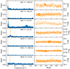 |
Fig. A.1. Strongest periodic signals in time-series photometry. Left panels: Lomb-Scargle periodograms of our target stars, based on OGLE data. The orange line shows the frequency at which the highest power is achieved, and the corresponding period is written in each panel. Right panels: Phase-folded light curves of I-band magnitudes, adopting the periods given in the left panels. |
RV measurements of SMC AB 1.
Same as Table A.1, but for SMC AB2.
Same as Table A.1, but for SMC AB4.
Same as Table A.1, but for SMC AB9.
Same as Table A.1, but for SMC AB10.
Same as Table A.1, but for SMC AB11.
Same as Table A.1, but for SMC AB12.
Overview of the OGLE-III and OGLE-IV time-series photometry data that was analyzed in this work.
Appendix B: Detection probabilities
B.1. More detection probability figures
Figure B.1 is the same as Fig. 6 except that it takes eccentricity into account. Specifically, eccentricities were drawn from a flat distribution between e = 0 and e = 0.9. The argument of periastron is given a random orientation for each mock binary.
We performed another experiment in which we tried to match the observed ΔRV value of SMC AB 9 with binary motion, rather than using a ΔRV cutoff. This is illustrated in Fig. B.2. We first estimate the error on the observed ΔRV by simulating our observing campaign of SMC AB9 105times. We give each RV measurement a random Gaussian offset based on its σCCF, which causes a modest spread around the originally measured ΔRV value (black line in Fig. B.2). The observed ΔRV error is then inferred from fitting a Gaussian to the distribution of ΔRV values. We then compare this with ΔRV values from a mock binary with a certain orbital period and companion mass (e.g., Porb = 251.2 d and a 5 M⊙ in Fig. B.2), for which we assume that the only uncertainty affecting ΔRV is given by σCCF. Finally, we define pm as the fractional overlap of the black and orange ΔRV histograms (shaded orange region in Fig. B.2). Figure B.3 shows the pm values that we obtain over the whole binary parameter space in the range 0 ≤ log(Porb/d)≤3.5 and 1 ≤ M2/M⊙ ≤ 40.
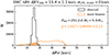 |
Fig. B.2. Histograms of simulated ΔRV values for SMC AB9. We show the scattered observations and a mock binary with Porb = 501.2 d and a 5 M⊙ companion. |
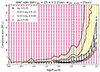 |
Fig. B.3. Same as Fig. 6, but instead of calculating the probability that ΔRVsim exceeds the threshold value, ΔRVobs, we calculate the probability, pm, that ΔRVsim matches ΔRVobs (see the main text for details). |
Probabilities that binaries caused a larger ΔRV than observed.
B.2. Integrated detection probabilities
We can calculate the weighted average detection probability  by summing over all the probabilities pij we calculated (shown in Fig. 6 and similar figures in Appendix B.1), weighted by the individual weights wP, i (based on the orbital period) and wM, j (based the companion mass) and normalized by the sum of the individual weights:
 (B.1)
(B.1)
We sum from i = 1 to i = 36 because we explore 36 values for log(Porb/d) in Sect. 5, and we sum over 40 values of j because we explore 40 values for the companion mass. For flat probability distributions, individual weights wP, i and wM, j have a value of unity if the orbital period and companion mass are within the range we consider (else they are zero). In two cases ( and
and  ), we use non-flat probability distributions of log(Porb/d) and M2, which are based on previous binary populations synthesis works (Langer et al. 2020; Renzo et al. 2019). Below, we describe how we obtain these probability distributions.
To calculate  , we used the orbital period and mass ratio distributions obtained from the population synthesis calculations of Langer et al. (2020) for O star–BH binaries in the LMC (cf. their Figs. 4 and 6). The mass transfer in most of the underlying detailed binary models was highly inefficient. Since BH formation kicks were neglected in this work, the predicted parameters of the O star–BH binaries are expected to be similar the those of their O star-WR binaries progenitors.
We also investigate the theoretical orbital period and mass ratio distribution based on models with conservative mass transfer (Renzo et al. 2019), which produce wider binaries (more difficult to detect) with more massive companions (easier to detect). To calculate  , we used Engauge Digitizer to tabulate the semimajor axis distribution of M > 15 M⊙ accretor stars in Fig. D.2 of Renzo et al. (2019). We converted this to an orbital period distribution assuming typical masses of MWR = 20 M⊙ and Mcomp = 35 M⊙. This led to a period distribution with peaks around log(Porb/d) = 1 and log(Porb/d) = 2.8, going toward zero for log(Porb/d) < 0.2 and log(Porb/d) > 3.5. The companion mass distribution was estimated using the following assumptions: (i) upon interaction, a 40 M⊙ star gets stripped to a 20 M⊙ WR star; (ii) the minimum value of qcrit = 0.4 for stable mass transfer adopted by Renzo et al. (2019); (iii) a fully conservative mass transfer, that is, the 20 M⊙ lost by the WR star ends up on the accretor star; and (iv) a flat initial mass ratio distribution. This leads to a flat companion mass distribution between 36 M⊙ and 60 M⊙. To take a slightly conservative approach to estimating
  and to bring this in line with the parameter space explored before, we instead adopt a flat companion mass distribution between 30 M⊙ and 40 M⊙.
We find that  and
and  are even higher (∼98%) than
  (∼90%). The reason is that the binary models do not predict very low mass companions, and the binary models of Langer et al. (2020) avoid orbital periods above log(Porb/d) = 3.
For both  and
and  , we repeat the exercise but we take the systems with Porb < 30 d out of the distribution, with the motivation that all of these might have been detected already. This shifts the probability distributions of the remaining binaries toward higher periods and hence the values for
  and
and  become smaller. However, we still find average detection probabilities in excess of 95%.
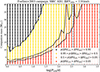 |
Fig. B.10. Probability that binary-induced motion exceeds the observed ΔRVobs for measurements performed by F03 on SMC AB1. |
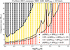 |
Fig. B.11. Same as Fig. B.10, but for SMC AB2. |
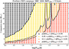 |
Fig. B.12. Same as Fig. B.10, but for SMC AB4. |
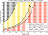 |
Fig. B.13. Same as Fig. B.10, but for SMC AB9. |
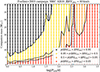 |
Fig. B.14. Same as Fig. B.10, but for SMC AB10. |
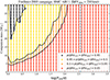 |
Fig. B.15. Same as Fig. B.10, but for SMC AB11. |
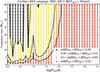 |
Fig. B.16. Same as Fig. B.10, but for SMC AB12. In this case, ΔRVobs is based on measurements of Foellmi (2004). |
Same as Table B.1, but instead of only considering circular orbits we consider eccentric orbits with eccentricities that are drawn from a flat distribution between 0 and 0.9.
Same as Table B.1, but for the observing campaign of Foellmi et al. (2003a) and, for SMC AB12, Foellmi (2004).
All Tables
Median ΔRV and σRV measured in our campaign for our seven target stars, using different lines.
Overview of the OGLE-III and OGLE-IV time-series photometry data that was analyzed in this work.
Same as Table B.1, but instead of only considering circular orbits we consider eccentric orbits with eccentricities that are drawn from a flat distribution between 0 and 0.9.
Same as Table B.1, but for the observing campaign of Foellmi et al. (2003a) and, for SMC AB12, Foellmi (2004).
All Figures
|
Fig. 1. Normalized 100 Å wide cutouts of the co-added VLT-UVES spectrum of SMC AB9. For reference, the blue arrow indicates the wavelength shift resulting from a 300 km/s velocity shift at the central wavelength of each panel. |
| In the text | |
|
Fig. 2. Illustration of the cross-correlation method. Top: N V 4604, 4620 Å doublet that is used for cross-correlation, shown for SMC AB9. The co-added spectrum as well as the spectrum that was taken on observing night 0 are displayed. For reference, we also show spectrum 0 shifted by 40 km/s. The spectra are normalized and then vertically shifted such that the integrated flux in the shown wavelength range is zero. Bottom: CCFs of the N V 4604, 4620 Å doublet for the co-added template spectrum and the six individual spectra that were taken. For this figure, the spectra were not corrected for barycentric motion. |
| In the text | |
|
Fig. 3. RV measurements based on UVES spectra taken on different nights. The first of the six spectra of our observing campaign was taken on observation night 0. The time interval in days between different observation nights is written at the bottom of the subplots. For SMC AB1, 2, and 4, we also show measurements based on the preexisting UVES spectra of Marchenko et al. (2007) (they are the data from observation nights −2 and −1). In this work we opted to use the N V lines, which are shown with thicker lines. |
| In the text | |
|
Fig. 4. Similar to Fig. 3, but showing RV measurements from a previous monitoring campaign (F03) and the three previous RV measurements of SMC AB12 from Foellmi (2004). These measurements have been shifted by the previously measured average RV for each star. The center and right plots on the bottom row are cumulative probability distributions. |
| In the text | |
|
Fig. 5. Normalized cutouts of the co-added VLT-UVES spectrum of SMC AB1 (black lines). We also show the spectrum taken on observing night 4 (orange lines), corrected for barycentric motion. |
| In the text | |
|
Fig. 6. Color-coded probability, p(ΔRVsim > ΔRVobs), that binary-induced motion would lead to a RV variation exceeding the observed ΔRVobs in SMC AB9, for different combinations of orbital period, Porb, and companion mass (see the main text for details). The higher this probability is, the less likely the source is an undetected binary. The dashed blue vertical line indicates Porb = 1 yr. |
| In the text | |
|
Fig. 7. Correlation of the time interval, Δtsucc, between two successive RV measurements and their observed ΔRVsucc. Top: The black crosses represent measurements taken in this work and in Marchenko et al. (2007). Middle: Measurements of a simulated population of long-period binaries with orbital periods between 1 and 10 years (see the main text for details), shown as colored dots. For clarity, we show only 2 of the 100 000 simulated observing campaigns. Bottom: Histogram of the 100 000 fitted slopes. The two vertical lines indicate the values of the two examples shown in the middle panel. |
| In the text | |
|
Fig. 8. RVs of our targeted WR stars (vertical orange lines; the shaded region indicates the error margin). The blue histograms show the RVs of Gaia DR3 sources in a 15′ radius. |
| In the text | |
|
Fig. 9. Velocities transverse to the line of sight. Our targeted WR stars are shown in orange, and binary SMC WR stars are shown in magenta. The shown errors are obtained from proper motion errors. Gaia DR3 sources in a 5′ radius are shown in blue. |
| In the text | |
|
Fig. 10. Initial mass–final mass relations for SMC stars. Data points of SMC WR stars are shown with circles (based on Hainich et al. 2015) and squares (based on Martins et al. 2009; Martins 2023), the numbers indicating their identifier (e.g., 1 for SMC AB1). The gray shaded region indicates He core masses at the terminal-age main sequence (MHe core, TAMS) from evolutionary models of Schootemeijer et al. (2019), for overshooting values between 0.22 and 0.44. The colored lines show the following relations from literature: MIST (Dotter 2016; Choi et al. 2016), Schn23 (Schneider et al. 2023), Bonn (Schootemeijer et al. 2019), Geneva (Georgy et al. 2013), SEVN+PARSEC (Iorio et al. 2023, overshooting value of 0.4), Belc10 (Belczynski et al. 2010, data taken from Fig. 2 of Banerjee et al. 2020), MOBSE (Giacobbo et al. 2018), and Hurl00 (Hurley et al. 2000, data taken from Fig. 1 of Belczynski et al. 2010). |
| In the text | |
|
Fig. A.1. Strongest periodic signals in time-series photometry. Left panels: Lomb-Scargle periodograms of our target stars, based on OGLE data. The orange line shows the frequency at which the highest power is achieved, and the corresponding period is written in each panel. Right panels: Phase-folded light curves of I-band magnitudes, adopting the periods given in the left panels. |
| In the text | |
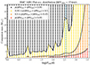 |
Fig. B.1. Same as Fig. 6, but assuming a flat eccentricity distribution instead of circular orbits. |
| In the text | |
|
Fig. B.2. Histograms of simulated ΔRV values for SMC AB9. We show the scattered observations and a mock binary with Porb = 501.2 d and a 5 M⊙ companion. |
| In the text | |
|
Fig. B.3. Same as Fig. 6, but instead of calculating the probability that ΔRVsim exceeds the threshold value, ΔRVobs, we calculate the probability, pm, that ΔRVsim matches ΔRVobs (see the main text for details). |
| In the text | |
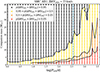 |
Fig. B.4. Same as Fig. 6, but for SMC AB1. |
| In the text | |
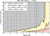 |
Fig. B.5. Same as Fig. 6, but for SMC AB2. |
| In the text | |
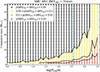 |
Fig. B.6. Same as Fig. 6, but for SMC AB4. |
| In the text | |
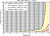 |
Fig. B.7. Same as Fig. 6, but for SMC AB10. |
| In the text | |
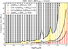 |
Fig. B.8. Same as Fig. 6, but for SMC AB11. |
| In the text | |
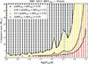 |
Fig. B.9. Same as Fig. 6, but for SMC AB12. |
| In the text | |
|
Fig. B.10. Probability that binary-induced motion exceeds the observed ΔRVobs for measurements performed by F03 on SMC AB1. |
| In the text | |
|
Fig. B.11. Same as Fig. B.10, but for SMC AB2. |
| In the text | |
|
Fig. B.12. Same as Fig. B.10, but for SMC AB4. |
| In the text | |
|
Fig. B.13. Same as Fig. B.10, but for SMC AB9. |
| In the text | |
|
Fig. B.14. Same as Fig. B.10, but for SMC AB10. |
| In the text | |
|
Fig. B.15. Same as Fig. B.10, but for SMC AB11. |
| In the text | |
|
Fig. B.16. Same as Fig. B.10, but for SMC AB12. In this case, ΔRVobs is based on measurements of Foellmi (2004). |
| In the text | |
Current usage metrics show cumulative count of Article Views (full-text article views including HTML views, PDF and ePub downloads, according to the available data) and Abstracts Views on Vision4Press platform.
Data correspond to usage on the plateform after 2015. The current usage metrics is available 48-96 hours after online publication and is updated daily on week days.
Initial download of the metrics may take a while.