| Issue |
A&A
Volume 691, November 2024
|
|
|---|---|---|
| Article Number | A174 | |
| Number of page(s) | 14 | |
| Section | Stellar structure and evolution | |
| DOI | https://doi.org/10.1051/0004-6361/202450354 | |
| Published online | 13 November 2024 | |
Exploring the boundary between stable mass transfer and L2 overflow in close binary evolution
1
Argelander-Institut für Astronomie, Universität Bonn, Auf dem Hügel 71, 53121 Bonn, Germany
2
Max-Planck-Institut für Radioastronomie, Auf dem Hügel 69, 53121 Bonn, Germany
⋆ Corresponding author; chr-schuermann@uni-bonn.de
Received:
12
April
2024
Accepted:
26
July
2024
The majority of massive stars resides in binary systems, which are expected to experience mass transfer during their evolution. However, the conditions under which mass transfer leads to a common envelope, and thus possibly to a merging of both stars, are currently only poorly understood. The main uncertainties arise from the possible swelling of the mass gainer and from angular momentum loss from the binary system during non-conservative mass transfer. We have computed a dense grid of detailed models of stars that accrete mass at constant rates to determine the radius increase that is due to their thermal disequilibrium. While we find that models with an accretion that is faster than the thermal timescale expand in general, this expansion remains quite limited in the intermediate-mass regime even for accretion rates that exceed the thermal timescale accretion rate by a factor of 100. Our models of massive stars expand to extreme radii under these conditions. When the accretion rate exceed the Eddington accretion rate, our models expand rapidly. We derived analytical fits to the radius evolution of our models and a prescription for the boundary between stable mass transfer and L2 overflow for arbitrary accretion efficiencies. We then applied our results to grids of binary models adopting various constant mass-transfer efficiencies and angular momentum budgets. We find that the first parameter affects the outcome of the Roche-lobe overflow more strongly. Our results are consistent with detailed binary evolution models and often lead to a smaller initial parameter space for stable mass transfer than do other recipes in the literature. We used this method to investigate the origin of Wolf-Rayet stars with O star companions in the Small Magellanic Cloud, and we found that the efficiency of the mass transfer process that led to the formation of the Wolf-Rayet star was likely lower than 50%.
Key words: binaries: close / binaries: general / stars: evolution / stars: massive / stars: Wolf-Rayet
© The Authors 2024
 Open Access article, published by EDP Sciences, under the terms of the Creative Commons Attribution License (https://creativecommons.org/licenses/by/4.0), which permits unrestricted use, distribution, and reproduction in any medium, provided the original work is properly cited.
This article is published in open access under the Subscribe to Open model. Subscribe to A&A to support open access publication.
1. Introduction
Binary stars play a key role in stellar physics because most of the massive stars, which enrich the Universe with elements and shape star-forming galaxies by their energy output, are part of a binary system (Vanbeveren et al. 1998; Sana et al. 2012; Moe & Di Stefano 2017). Such systems may lead to powerful phenomena such as X-ray pulsars (Tauris & van den Heuvel 2006) and gravitational-wave events (Tauris & van den Heuvel 2023). Interacting binaries are an important site of stellar nucleosynthesis (de Mink et al. 2009b; Margutti & Chornock 2021), and low-mass interacting binaries are possible progenitors of Type Ia supernovae, which are essential for the mapping of the Universe (Riess et al. 1998; Schmidt et al. 1998; Perlmutter et al. 1999).
Close binaries interact sooner or later (Sana et al. 2012), but the result that arises when one component fills its Roche lobe is still debated (Langer 2012; Marchant & Bodensteiner 2024). A Roche-lobe overflow (RLO), in which material is steadily transferred from one star to the other (e.g. Kippenhahn & Weigert 1967), is thought to lead to a stripped star in the form of a hot sub-dwarf (Shenar et al. 2020a; Bodensteiner et al. 2020) or to a Wolf-Rayet (WR) star (Langer 1989; Wellstein et al. 2001) and a mass gainer that was spun up to fast rotation when the tides were negligible (de Mink et al. 2013; Wang et al. 2020), which is observable as a Be star (Rivinius et al. 2013). When the RLO is dynamical unstable or the two components evolve into contact, a common envelope is formed, which may be ejected (Kruckow et al. 2016) or drives the system towards a stellar merger (Ivanova et al. 2013; Schneider et al. 2019). Even when this scenario is avoided, it is unclear how much of the material that is lost by the donor star is accreted by its companion (de Mink et al. 2007) and how much angular momentum is drained from the system by the ejected material (Soberman et al. 1997).
Several studies have addressed these questions. A classical approach is to determine the mass-radius exponent of stellar models, as was done for instance by Hjellming & Webbink (1987) for polytropes, for more realistic stellar models by Hjellming (1989b,a), and most recently, by Ge et al. (2010, 2015, 2020). Wellstein et al. (2001) examined the formation of contact in conservative detailed binary evolution models. Langer et al. (2020), Wang et al. (2020), Sen et al. (2022) determined the accretion efficiency by letting the accretor take on mass until it reached critical rotation, and they used an energy criterion to determine the outcome of an RLO.
Kippenhahn & Meyer-Hofmeister (1977) and Neo et al. (1977) showed that the accretor expands when the inflow of matter is too fast (see also Ulrich & Burger 1976; Flannery & Ulrich 1977; Packet & De Greve 1979; Fujimoto & Iben 1989). When this expansion is large enough for the accretor to also fill its Roche lobe, the formation of a common envelope is expected, and after further expansion, this material leaves the binary at the second Lagrange point (L2 overflow), which is expected to lead to the merger of the two stars as the expelled material drains a large amount of angular momentum from the system (Nariai & Sugimoto 1976). Pols et al. (1991) inferred from the work of Kippenhahn & Meyer-Hofmeister (1977) that the accretor does not expand significantly as long as its accretion rate remains lower than ten times its thermal timescale accretion rate. This approach was commonly used in many binary population studies (e.g. Hurley et al. 2002; Shao & Li 2014, 2016; Vigna-Gómez et al. 2018; van Son et al. 2022), where the mass gain of the accretor was often limited by the thermal timescale accretion rate when the mass transfer rate exceeded this value (see Portegies Zwart & Verbunt 1996 and Toonen et al. 2012 for a more detailed approach). Other works did not consider the reaction of the accretor, and adopted more ad hoc merger criteria (e.g. Belczynski et al. 2002, 2008; Kruckow et al. 2018).
In the past decades, powerful codes such as that of Eggleton (1971, 1972, 1973, Eggleton et al. (1973), the Bonn evolutionary code (BEC, Heger et al. 2000; Yoon et al. 2006; Brott et al. 2011), the Brussels codes STAREVOL and BINSTAR (Siess et al. 2000; Siess 2006; Palacios et al. 2006; Siess & Arnould 2008; Davis et al. 2013; Deschamps et al. 2013; Siess et al. 2013), and Modules for Experiments in Stellar Astrophysics (MESA, Paxton et al. 2011, 2013, 2015, 2018, 2019) were developed for the detailed modelling of both single and binary stars. However, it is still a large effort even today to model a complete stellar population with these one-dimensional approaches. Therefore, rapid population synthesis codes have been developed that approximate the evolution of binary systems either by analytic fits (e.g. Hurley et al. 2002) or by interpolating precalculated single-star models (e.g. Kruckow et al. 2018). Thus, it is one aim of this study to provide a practical and efficient method for determining the outcome of an RLO without the need for detailed modelling.
Our study consists of two parts. In Sect. 1, we analyse a generic set of detailed accreting single-star models to determine an accurate and practical description of their radius evolution as a function of the relevant parameters. In the second part (Sect. 3), we apply our results to grids of binary models that we also compare to observations. Throughout the paper, we compare our simplified models with detailed binary evolution models.
2. Accretion onto main-sequence stars
2.1. Method
We calculated detailed single-star models with a Small Magellanic Cloud (SMC) metallicity with initial chemical compositions as in Brott et al. (2011, their Tables 1 and 2, i.e. ZSMC = 0.0021) and custom-built OPAL opacities (Iglesias & Rogers 1996) in line with these abundances. The initial masses Mi of the models were 1, 1.5, 2, 3, 5, 7, 10, 15, 20, 30, 50, 70, and 100 M⊙, and we assumed various constant accretion rates Ṁ (see Fig. 1 top and Sect. 4) using MESA version 10108 (Paxton et al. 2011, 2013, 2015, 2018). We applied the Ledoux criterion for convection and used the standard mixing-length theory with αml = 1.5. We followed Schootemeijer et al. (2019) and Hastings et al. (2021) and used semi-convection with αsc = 10 and a mass-dependent step-overshooting. We assumed thermohaline mixing following Cantiello & Langer (2010) with αth = 1. We simplified our models by treating them as non-rotating. After the stellar models relaxed onto the main sequence, they were subjected to a constant accretion of material that carried the same entropy as the uppermost mass shell of the model. We let the models accrete until they had quintupled in mass, at which point we terminated the calculations.
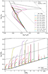 |
Fig. 1. Evolution of our accreting single-star models. Top: Evolution of the 5 M⊙ models in the HRD for different accretion rates (indicated by colour). Stably swelling models are shown with solid lines, and unstable models are plotted with dashed lines. We also show the ZAMS (black) and various lines of a constant radius (grey). Bottom: Radius of accreting models as a function of mass until they reach maximum radius. For each initial mass, the colours are the same as in the corresponding HRDs (top panel and Sect. 4). Models that become unstable are indicated by dashed lines. Some are so short that they are hardly visible. The ZAMS radius is shown in black. |
2.2. Results
2.2.1. Behaviour of accreting main-sequence star models
We show the tracks of our 5 M⊙ models in the Hertzsprung–Russell diagram (HRD) in Fig. 1 (top), which are typical for our model grid. We indicate the different adopted accretion rates by colour. The corresponding diagram for the other initial masses available online (see Sect. 4). In the bottom panel, we show the radius evolution as a function of the model mass M up to its maximum radius.
The stellar models with lower accretion rates follow a common pattern. At the onset of accretion, they briefly evolve to the left of the zero-age main sequence (ZAMS) as a hydrodynamic response to the accretion, only to rapidly increase their radius R thereafter (except for the lowest accretion rates). The increase in radius is stronger for higher accretion rates. After reaching a maximum radius Rmax at a mass MR = Rmax, the models again contract towards the ZAMS. They evolve from there along the ZAMS as they still accrete material. We call these models stable models or models with stable swelling.
The two models with the highest accretion rates of Fig. 1 (top; yellow and cyan lines) show a different evolution from the stable models because their lines are so short that they are barely visible in the two plots. These models barely accrete any mass and terminate shortly after the onset of the accretion because of numerical problems, as the time step becomes unreasonably small. We call these models unstable models or models with unstable swelling.
We observe the same patterns for models with other masses (online material, Sect. 4). The higher the accretion rate, the larger the maximum radius of the models, and beyond a certain accretion rate, the models terminate because of numerical problems. For initial masses above 10 M⊙, the unstable models show a strong increase in radius before they terminate (Fig. 1, bottom, dashed lines). This extends the interpretation of the unstable models to the description that above a certain accretion rate, a small increase in mass causes the star to expand by a very large amount. We consider, for instance, the models with an initial mass of 15 M⊙ in Fig. 1 (bottom). From 1 ⋅ 10−3 M⊙/yr (blue) to 3 ⋅ 10−3 M⊙/yr (green) the swelling becomes stronger, but at an accretion rate of 6 ⋅ 10−3 M⊙/yr (red), the mass-radius curve becomes nearly vertical. Furthermore, for initial masses above 10 M⊙, we find that a stable radius increase becomes less possible with increasing mass, and from 30 M⊙ on, the models either accrete stably along the ZAMS or become unstable.
Between the stable and unstable regimes, we find three borderline models: 2 M⊙ with Ṁ = 2 · 10−4 M⊙/yr, 7 M⊙ with Ṁ = 2 · 10−3 M⊙/yr, and 10 M⊙ with Ṁ = 2.5 · 10−3 M⊙/yr. These models have in common (in contrast to the other stable ones) that they reach their maximum radius as red (super) giants and that their tracks in the HRD depict a lower curvature at maximum radius. Fig. 1 (bottom) shows that the three borderline models reach the largest radii of all stable models of the same initial mass, and they show a plateau in this. We assume that the unstable models would show the same behaviour as the borderline models if they could be calculated further, which is supported by the binary models presented in Sect. 2.3.2.
We can understand whether a model accretes stably by considering the Eddington accretion rate, given by
where c is the speed of light, R is the stellar radius, and κ is the opacity (Webbink et al. 1985; Tauris & van den Heuvel 2023). By assuming R ∝ M0.6, which fits our ZAMS models well (Kippenhahn et al. 2013), and κ = 0.34 cm2/g, which is a good approximation for M > 10 M⊙, we find
![$$ \begin{aligned} \dot{M}_{\rm Edd} \approx \left[1.2\cdot 10^{-3} \,M_\odot /\mathrm{yr}\right] \cdot \left(\frac{M}{\,M_\odot }\right)^{0.6}. \end{aligned} $$](/articles/aa/full_html/2024/11/aa50354-24/aa50354-24-eq2.gif)
In Fig. 2 we show the initial mass and the adopted accretion rate of our models. The opacity of twice the electron-scattering value, which approximates the total opacity in the outer envelope of our models, matches the boundary between the stable and unstable models well. This means that our models become unstable when the accretion rate exceeds the Eddington accretion rate of the accretor. The reason might be that the material at the surface of a star close to its Eddington limit is barely bound. Sanyal et al. (2015, 2017) found that stars like this can inflate to large radii, and it therefore appears to be likely that they are pushed close to their Hayashi line (see Sects. 2.3.1 and 3.1).
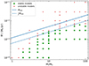 |
Fig. 2. Initial mass and adopted accretion rate for our stable (green) and unstable (red) models. Not all models are shown because we focus on the boundary between stable and unstable models at high masses. The blue lines indicate the Eddington accretion rate assuming electron-scattering opacity. |
2.2.2. Analytic fits
To describe the response of the stellar models to accretion, Fig. 3 shows a synopsis of our models. We express the accretion rate in terms of the logarithmic ratio,
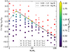 |
Fig. 3. Maximum radius of accreting models as a function of initial mass and ratio of the thermal and mass-transfer timescales. Unstable models are shown in red. Special symbols are used for selected accretion rates. The two black lines distinguish between stable and unstable models. |

of the thermal timescale τKH and the mass-gain timescale τṀ at the onset of accretion, which are defined as

where L is the luminosity, and G is the gravitational constant (Hansen et al. 2004; Kippenhahn et al. 2013). We find that the boundary between stable and unstable models can be described by two simple lines, which are given by
For masses above 2 M⊙, we find that our models become more unstable with increasing initial mass. Models below this show the opposite trend. Moreover, the closer to the boundary a model of a given initial mass, the larger its maximum radius. For a fixed t, the maximum radius is minimum around Mi = 2 M⊙. Near the boundary, the maximum radii are up to 100 times larger than the ZAMS radii. For models with  , the swelling is negligible.
In order to incorporate our results into a rapid binary population synthesis code, we fitted simple functions to the logarithmic radius increase r = log Rmax/Ri and the mass increase to reach the maximum radius m = MR = Rmax/Mi as functions of the initial mass Mi and the logarithmic timescale ratio t. For the function r, we required that r(t = 0) = 0 and that it reached values of 2 at the boundary towards the unstable models, which roughly corresponds to the radius increase of the three borderline models (1.9, 2.3, and 2.3). While a systematic search for the mass-dependent borderline accretion rate is possible (Lau et al. 2024), the exact value is not important for practical applications.
We find a good fit for Rmax with the function
![$$ \begin{aligned} r(\log M_{\rm i}, t) = 2 \cdot \frac{\exp {\left[(a\log M_{\rm i}+b) \frac{t}{3-1.5\log M_{\rm i}} \right]}-1}{\exp {\left[a\log M_{\rm i}+b\right]}-1}, \quad 0<t<t_{\rm max}, \end{aligned} $$](/articles/aa/full_html/2024/11/aa50354-24/aa50354-24-eq8.gif)
with the parameters a and b given in Table 1. The logarithmic timescale ratio t is not divided by tmax as in Eq. (6), but only by the second line of the formula. We show the values of the detailed models as well as our fit function in Fig. 4. The data and fit agree well because the root mean square relative deviation1 and the maximum relative deviation of Rmax and MR = Rmax are reasonably small (Table 1).
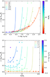 |
Fig. 4. Logarithmic radius increase r of accreting models as a function of initial mass and ratio of the thermal and mass-transfer timescale together with our fit (lines) for selected initial masses (top) and for selected timescale ratios (bottom). |
For the mass at the maximum radius, we find that the linear function given by

fits well. The parameters a, b, c are listed in Table 1. The values of the detailed models and the fit are shown in Fig. 5.
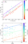 |
Fig. 5. Mass at which accreting models reach their largest radius as a function of initial mass and ratio of the thermal and mass-transfer timescale together with our fit for selected initial masses (top) and for selected timescale ratios (bottom). |
2.3. Discussion
In this section, we discuss the uncertainties of our prescription (Sect. 2.3.1) and compare them with detailed binary models (Sect. 2.3.2) and previous works (Sect. 2.3.3).
2.3.1. Uncertainties
In our models, we omitted stellar rotation for simplicity. However, rotation is a ubiquitously observed in stars (Maeder & Meynet 2000; Langer 2012). It has several effects on stars. First of all, the stellar surface is deformed by the centrifugal force (e.g. Kippenhahn et al. 2013). This effect can increase the equatorial radius by a factor of up to 1.5. This number is within the uncertainty of our prediction for the accretion-induced swelling (Sect. 2.2). Moderate rotation does not alter stellar evolution much (Brott et al. 2011; Choi et al. 2016), so the expected corotation in close binaries (de Mink et al. 2009a) and the fast-rotating branch of the main sequence (Dufton et al. 2013; Wang et al. 2020) are not affected.
On the other hand, it is generally accepted that mass transfer leads to a spin-up of the accretor star to close to critical rotation (de Mink et al. 2013). Packet (1981) showed that only a small amount of matter is required to spin up the star when no tidal breaking (Zahn 1977) acts. Therefore, the accretors in all but the closest mass-transferring binaries can be expected to rotate rapidly (Wang et al. 2020; Sen et al. 2022). As a result of the centrifugal force, the equatorial radius of a rapid rotator is increased by up to 50% (Gagnier et al. 2019). While this is a moderate radius increase compared to the accretion-induced inflation discussed above, it adds to the uncertainties in the boundary between stable and unstable mass transfer.
It is likely that the mass-gainer accretion rate in mass-transferring binaries is not constant, but varies with time. For a strongly varying accretion rate, the assumption we make for Eq. (9) would no longer be valid. In the models of Langer et al. (2020), Wang et al. (2020), and Sen et al. (2022), the effective accretion rate varied because it depends on the rotation rate of the mass gainer. A variation in the mass-transfer rate can also be induced by the evolution of the Roche-lobe radius (Kippenhahn & Weigert 1967; Tauris & van den Heuvel 2023). On the other hand, strong oscillations of the mass transfer and accretion rate appear unlikely, such that focusing on the time interval with the most efficient accretion may yield a valid approximation.
We assumed that the material arriving at the accretor has the same entropy as its surface. This assumption is justified for accretion rates below the thermal timescale accretion rate, that is, for t < 0 (Eq. (3)) because in this case, any excess energy is radiated away quickly (Paxton et al. 2015). For t > 0, the impact of the accretion stream (Ulrich & Burger 1976; Shaviv & Starrfield 1988), or boundary layer heating in the case of disk accretion onto a sub-critically rotating star (e.g. Steinacker & Papaloizou 2002), may deposit hot material onto the star faster than the additional heat can be drained. The energy released by these processes is related to the gravitational energy gain of the infalling matter (which we neglected), and it is therefore comparable to but does not greatly exceed the energy released by the gravitational compression of the star by the weight of the accreted mass (which we included). We therefore do not expect a qualitative impact of these effects on our results.
Finally, we note that we explored the effects of accretion on the upper main sequence, and our results cannot be extrapolated into the regime of low-mass main-sequence stars. Zhao et al. (2024) have shown that low-mass main-sequence stars with deep convective envelopes, as well as fully convective main-sequence stars, undergo shrinkage upon accretion, even for accretion rates that exceed the thermal timescale accretion rate by many orders of magnitude.
2.3.2. Comparison with detailed binary models
To validate our results, we compared our fits with detailed binary models undergoing RLO calculated with MESA (see Sect. 2.1). The adopted initial masses and initial periods are listed in Table 2. We used the same physical assumptions as in Sect. 2.1, and the structure of both binary components was calculated in parallel with the evolution of the orbit. The models were assumed to be non-rotating because we are not interested in the radius increase due to this effect. We assumed a constant accretion efficiency of ε = 50% and that the ejected material carried the specific angular momentum of the accretor (Soberman et al. 1997). We used the mass-transfer scheme roche_lobe. To be able to measure the maximum accretor radius, we allowed the accretor to overfill its L2 volume without losing mass or terminating the calculation.
Properties of our detailed binary models.
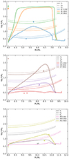 |
Fig. 6. Mass-radius evolution (solid line) of detailed accretor models for different initial periods (colour) and initial accretor masses (top 4 M⊙, middle 6 M⊙, bottom 8 M⊙). The donor always has an initial mass of 10 M⊙. The size of the accretor Roche lobe and L2 sphere are shown as dashed and dotted lines. We used crosses to indicate the maximum of the mass-radius curve (Rmax, MR = Rmax) according to Eqs. (7) and (8), based on the maximum mass-transfer rate of the detailed model. The plusses indicate the same, but for an estimate of the mass-transfer rate based on the conditions just before the RLO (Eq. (9)). When a symbol is placed at a high radius but at the initial mass of the model, the model is expected to swell unstably, and the radius is the Hayashi radius (see Sect. 3.1). |
The mass-radius evolution of the accretors with an initial mass of 10 M⊙ is shown in Fig. 6 together with estimates according to Eqs. (7) and (8) based on the maximum mass-transfer rate of the models (crosses). In general, we find a satisfactory agreement. We typically miss the maximum radius by no more than a factor of 2. Models 2 (orange) and 3 (green) stay at large and relatively constant radii for a while, similar to the borderline models mentioned in Sect. 2.2.1. They also swell unstably according to Eqs. (7) and (8). Models 4, 8, and 12 are not shown because the calculations terminated because of numerical problems (time-step limit) shortly after the onset of RLO. Typically, our recipe yields smaller accretor radii than in detailed calculations, which means that it is a rather conservative estimate of L2 overflow.
There are two main reason for the differences between our approach and the detailed models. Our fitting function (Sect. 2.2.2) is very steep, and thus, small uncertainties can lead to large changes in the resulting maximum radius. This could be improved with a denser model grid and a refined fit. Second, the accretion rate imposed by the donor is time dependent, and a notable deposition of material onto the mass gainer before the maximum mass-transfer rate is reached could change our prediction. Considering a time-dependent mass transfer rate is beyond the scope of our approach.
2.3.3. Comparison with previous work
Numerical experiments for accreting stars have been carried out by Kippenhahn & Meyer-Hofmeister (1977) and Neo et al. (1977). They arrived at the same qualitative result as our study: The maximum stellar radii increase as the accretion rate increases. When we compare the tracks in our HRDs with those of Kippenhahn & Meyer-Hofmeister (1977, their Figs. 1–3) and Neo et al. (1977, Fig. 1), we find that the evolutionary tracks of Neo et al. (1977), like ours, intersect for a given initial mass, but those of Kippenhahn & Meyer-Hofmeister (1977) do not. On the other hand, we find similarities between Fig. 4 of Kippenhahn & Meyer-Hofmeister (1977) and Fig. 4 of Neo et al. (1977) and our Fig. 1 (bottom), not only in the shape of the tracks, but also for the critical accretion rate. Neo et al. (1977) reported that an accretion rate greater than 4 ⋅ 10−3 M⊙/yr is required for a 20 M⊙ model to be unstable. We find a slightly lower rate of 3 ⋅ 10−3 M⊙/yr. Similarly, for the 5 M⊙ and the 10 M⊙ models, we also find slightly lower critical accretion rates compared to Kippenhahn & Meyer-Hofmeister (1977). The differences could be caused by the opacities that were used, firstly, because the old models did not include the iron-peak opacity, and secondly, we used a lower metallicity, which also enters the opacity and thus the Eddington limit.
Pols et al. (1991), Pols & Marinus (1994) stated that the response of the accretor becomes important when the thermal timescale exceeds the accretion timescale by a factor of ten, that is, for t = 1. In contrast, we find that the radius of the accretor already deviates from equilibrium when the accretion timescale is equal to the thermal timescale (t = 0), and the swelling becomes unstable at t = tmax. Our tmax is mass dependent, in contrast to their mass-independent limit of t = 1. However, these studies and subsequent work (e.g. Shao & Li 2014, 2016; Schneider et al. 2015) assumed that the unstable swelling leads to a reduced accretion efficiency and only to a merger when the ejected angular momentum is high enough.
Recently, similar studies were reported by Zhao et al. (2024) and Lau et al. (2024), who calculated accreting models at solar metallicity. Their models behaved qualitatively similar to our models. However, a close inspection reveals that our models swell less for the same accretion rate. For example, our 5 M⊙ model with Ṁ = 10−3 M⊙/yr reaches about 120 R⊙, while that of Lau et al. (2024, Z = 0.0142) swelled to around 500 R⊙ and that of Zhao et al. (2024, Z = 0.02) reached about 600 R⊙. This behaviour may be related to the metallicity dependence of the opacity (see Sect. 2.2.1). A higher metallicity increases the opacity, which in turn decreases the Eddington accretion rate. This means that for an increasing metallicity, the boundary between stable and unstable accretion moves to lower timescale ratios t. The magnitude of the shift is hard to estimate from the combined model data. The 5 M⊙ model of Zhao et al. (2024) with Ṁ = 10−3 M⊙/yr appears to be what we consider a borderline model. Our comparable model accretes stably, and our 5 M⊙ model with Ṁ = 1.5 · 10−3 M⊙/yr is unstable. We can estimate based on this that the shift of the boundary between stable and unstable accretion may be less than 0.2 dex from the SMC to solar metallicity. Lau et al. (2024) analysed their models, but fit their results with different parameters, so that a direct comparison is difficult. However, two common features are the double-exponential behaviour of the stably accreting models on the accretion rate, and the higher sensitivity of more massive models to the accretion rate. Other model assumptions, such as core overshooting and the mixing-length parameter, may also have an impact.
3. Predictions for L2 overflow
In this section, we apply our model for the swelling of the accretor star to model grids of binary systems. We follow the evolution of the accretor radius and its Roche radius. We then determine the conditions under which the accretor overfills its Roche lobe, leading at first to contact and with further overfilling to an L2 overflow. We assume that the latter leads to a merger of the two stars (Nariai & Sugimoto 1976).
3.1. Method
We modelled the binary systems in our grid based on detailed non-rotating single-star models computed with MESA version 10108 (Paxton et al. 2011, 2013, 2015, 2018). The initial masses were 8, 10, 15, 20, 30, 50, 70, and 100 M⊙, and the physical assumptions were identical to those in Sect. 2.1, unless otherwise stated. We used overshooting (αov = 0.33) and semi-convection (αsc = 1) as in Wang et al. (2020) to avoid central helium ignition in the Hertzsprung gap (Schootemeijer et al. 2019), as the following Case C behaves differently than Case B mass transfer, and to better compare our results with Wang (2022). We ran our models until central helium depletion and used them to model the evolution of the donor star. For the accretor star, we assumed no evolution, which is justified for mass ratios different from unity, and we interpolated between the ZAMS models to build a binary grid for each donor mass with mass ratios from 0.1 to 0.95 in steps of 0.05 and orbital periods from 10−0.5 d ≈ 0.3 d to 103.5 d ≈ 3000 d in steps of 0.25 dex.
For each combination of initial donor mass M1i, initial accretor mass M2i, and initial orbital period, we determined the Roche radius of the donor using the fit formula from Eggleton (1983). When the Roche radius was equal to the stellar radius of a hydrogen core-burning donor model (RLO Case A), we calculated the post-RLO donor mass M1f according to Schürmann et al. (2024, Eq. (4)). When the Roche radius was equal to the stellar radius of a hydrogen shell-burning model (RLO Case B) or a helium-burning model (RLO Case C), we used the helium core-mass of the donor as the post-RLO donor mass M1f.
Next, we determined the logarithmic timescale-ratio t (Eq. (3)). The thermal timescale of the accretor star is given by Eq. (4) using the ZAMS values. The mass-transfer timescale can be calculated using Eq. (5). Ṁ2 is given by by −ε Ṁ1, which in turn can be estimated by  . The mass-transfer efficiency ε was assumed to be constant during the RLO and was a free parameter. Thus, we find
For t < 0, the accretor remains in thermal equilibrium, as discussed in Sect. 2, and we describe its radius evolution during the RLO by linearly interpolating log R2i to log R2f between M2i and the final secondary mass M2f, where we took the radius of a ZAMS model of mass M2f for R2f. For 0 < t < tmax (Eq. (6)), we determined the parameters r and m (Eq. (7) and (8)). We modelled the time-dependent accretor radius linearly from log R2i at M2i to log Rmax = log R2i + r at MR = Rmax = mM2i, and from log Rmax = log R2i + r to log R2f between MR = Rmax = mM2i and M2f. We chose this piece-wise linearity in log R due to the rough piece-wise linear behaviour shown in Fig. 6. For t > tmax, we assumed that the accretor swelled until it reached the Hayashi lines. We modelled this by assuming a fixed effective temperature of log Teff/ K = 3.6 and by adopting an additional luminosity given by
which accounts for the gravitational energy release of the accreted matter. In general, we used this to limit the accretor radius. We thus derived a model for the accretor radius under accretion as a function of the current accretor mass.
Similar to the mass-transfer efficiency ε, the angular momentum budget of an RLO is not well understood. To describe it, we used the formalism of Soberman et al. (1997), which allows an analytical analysis of certain angular momentum budgets. In addition to their parameters α, the fraction of mass lost from the donor leaving the system with the specific orbital angular momentum of the donor, and β, the mass fraction lost from the donor leaving the system with the specific orbital angular momentum of the accretor, we introduce η for the material ejected with the specific orbital angular momentum of the binary system. These quantities are related as ε = 1 − α − β − η. Soberman et al. (1997) introduced a parameter A to describe the enhancement of the angular momentum loss at the donor by spin-orbit coupling. We used this as a general parameter to scale the angular momentum loss and also introduced B and H as scaling factors for the angular momentum loss similar to A. This caused the three angular momentum evolution exponents in Soberman et al. (1997) Eqs. (25) to (27) to take the form

We used Eq. (28) from Soberman et al. (1997) to determine the system semi-major axis as a function of the accretor mass, expressed by the mass ratio. With this, we used the formula of Eggleton (1983) to calculate the Roche radius of the accretor RRL2 over the course of the RLO and Eqs. (3.1) and (3.2) from Marchant (2017) to find the L2 equivalent-radius RL22. Finally, we calculated the maximum of log(R2/RRL2) and log(R2/RL2) during the RLO as a function of initial mass ratio and initial orbital period for a fixed donor mass, mass-transfer efficiency, and angular momentum budget. The sign of these tells us whether the accretor remains within its Roche lobe or if contact or even a L2 overflow occurs.
3.2. Results
We show in Fig. 7 the maximum ratio of the accretor radius to its Roche radius over the course of the RLO for a donor with a mass of 10 M⊙ (top) and 30 M⊙ (bottom) for a mass-transfer efficiency of 50%, assuming that the ejected material carries the specific orbital angular momentum of the accretor, as a function of initial mass ratio and initial orbital period. Red dots indicate that the accretor exceeds its Roche lobe, and blue dots show accretors that remain within their Roche lobe. In the 10 M⊙ model, the accretor avoids filling its Roche lobe and the system does not evolve to contact for low initial orbital periods and mass ratios greater than about 0.5. For longer periods and lower mass ratios, the opposite is true. Contact is also expected for very short orbital periods below about 0.3 d, but this region is almost completely excluded because the donor RLO is at the ZAMS. A similar pattern is observed for the L2 overflow, which is expected because the L2 radius is not larger than about 30% of the Roche radius.
We can explain why the accretors in systems with a low-mass ratio tend to evolve to contact by using the thermal timescale of the accretor. The lower the mass ratio, the lower the accretor mass and luminosity, and hence, the longer accretor thermal timescale and higher logarithmic timescale ratio t because no changes were made to the donor. The tendency for systems with long orbital periods to develop contact can be understood by the thermal timescale of the donor. A larger orbit implies a larger donor radius at the start of RLO, which implies a shorter donor thermal timescale and thus a higher mass transfer rate, resulting in a higher logarithmic timescale ratio t.
For the adopted angular momentum budget (material leaving the system carries the same specific angular momentum as the accretor), we find Case A and Case B systems that can avoid contact. The cyan line, which marks RLO at ZAMS, indicates the lower period limit for meaningful binary evolution. We expect that the accretor does not overfill its Roche lobe in systems with orbital periods longer than 3000 d, indicated by the dotted lines in the upper right corner, because this period corresponds roughly to the largest radius possible for our Hayashi-line models (Eq. (10)). However, this is hardly relevant as the donor is barely expected to grow large enough in radius to initiate an RLO at such a high initial orbital period.
For the 30 M⊙ donor, we find that that the region in which contact is avoided is smaller than in the 10 M⊙ model. In particular, almost no Case B system can avoid contact. It is a general trend that as the donor mass increases, fewer systems avoid contact. We explain this with Fig. 3. Higher donor masses imply higher accretor masses. For higher accretor masses, tmax approaches zero, which in turn shrinks the contact-avoidance region.
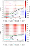 |
Fig. 7. Maximum ratio of the accretor radius to its Roche radius over the course of the RLO as a function of initial mass and initial orbital period in our simulated binary systems. Red means that the accretor star swells to become larger than its Roche lobe, and blue indicates that it remains within its Roche lobe. The black line marks the boundary between these, and in grey, we show the boundary for the L2 radius instead of the Roche radius. The dotted black and grey lines indicate a shift of ±0.5 dex in the two boundaries. The initial donor masses are 10 M⊙ (top) and 30 M⊙ (bottom), the mass-transfer efficiency is 50%, and we assume that the ejected material carries the specific orbital angular momentum of the accretor (α = η = 0, β = −ε, B = 1). We show the region in which RLO at ZAMS is expected (solid cyan line), the boundary between Case A and Case B (dashed green line), the onset of the donor convective envelope (dot-dashed orange line), and the critical mass ratio according to Ge et al. (2010, 2015, 2020), pink dotted line). Systems marked with numbers and black symbols are those for which we computed detailed models (see Table 2). The black circles indicate stable swelling without contact formation, squares stand for stable swelling but L2 overflow, and diamonds indicate unstable swelling with L2 overflow. |
In Fig. 8 we only show the boundary between contact and non-contact models, but for varying accretion efficiencies. At the highest efficiency, the contact-avoidance region is the smallest, and it grows with decreasing efficiency. This can be understood from Eq. (9), where t ∝ log ε. For the assumed angular momentum budget, we also find a limiting case given by completely non-conservative mass transfer (pink line). This indicates that for a fixed orbital period, systems with more extreme mass ratios than given by this line cannot avoid contact, and that this contact is caused by the orbital evolution of the system and not by the swelling of the accretor.
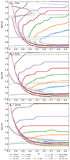 |
Fig. 8. Boundary between the contact-developing and the contact-avoiding models for different initial donor masses (from top to bottom, 10, 30, and 100 M⊙) assuming the ejected material carries the specific orbital angular momentum of the accretor (i.e. α = η = 0, β = −ε, B = 1). The colours indicate the assumed mass-transfer efficiency. The dashed lines show the boundary of L2 overflow, and the dotted lines represent the critical mass ratio for dynamical timescale mass transfer derived from Ge et al. (2010, 2015, 2020). |
In the online material (Sect. 4), we show the same as Fig. 8, but with different assumptions about the amount of angular momentum of the ejected material. When it carries twice the specific orbital angular momentum of the accretor, the main difference from the original case is that the boundary for unavoidable contact has moved to the right. When the ejected material carries the donor-specific orbital angular momentum, this boundary exists only towards short initial periods. The pattern remains that a higher mass-transfer efficiency implies more contact systems. When twice this angular momentum is ejected, most Case A mass transfers lead to contact for most mass-transfer efficiencies at low donor mass. When the ejected material carries the specific orbital angular momentum of the binary once or twice, a mixture of the above cases occurs. When no angular momentum is lost, the patterns resemble the case in which the ejected material carries the specific orbital angular momentum of the donor.
3.3. Discussion
In this section, we describe the uncertainties of our model (Sect. 3.3.1), compare it with detailed binary models in Sect. 3.3.2, apply our recipe to the WR stars in the SMC (Sect. 3.3.3), and compare our work with previous publications in Sect. 3.3.4.
3.3.1. Uncertainties
We have already described the uncertainties in modelling the swelling of the accretor in Sect. 2.3.1. In addition, the most important uncertainty for the model of the binary system probably is that we neglected the nuclear evolution of the accretor. This assumption is only realistic for systems with mass ratios different from unity, where the nuclear evolution of the more massive star is much faster than that of the companion. If this is not the case, stellar models predict that both the radius and luminosity of the star will have increased at the onset of accretion, and thus the thermal timescale of the accretor has decreased. This causes the logarithmic timescale ratio t to be lower given the same accretion rate. We therefore expect the accretor to expand less, which should increase the contact-avoidance region in Fig. 7 for mass ratios close to unity by shifting its upper boundary upwards.
The lack of nuclear evolution of the accretor also causes our models to avoid a reverse mass transfer and a mass transfer on post-main-sequence models. This is important for mass ratios very close to unity and/or Case A systems. When both stars have similar masses, the accretor star can complete its central hydrogen burning during or after the RLO, which is expected to result in a merger (Wellstein et al. 2001; Sen et al. 2022). For a Case A RLO, this is much more likely, even for mass ratios different from unity, since this type of mass transfer proceeds on the nuclear timescale (Pols 1994; Wellstein et al. 2001; Sen et al. 2022). A comparison of our Fig. 7 with the yellow shaded area of Fig. A.4 (left) of Wang (2022) suggests that at least half of the systems in the contact-avoiding region of Case A should undergo this effect.
Our adopted values for semi-convection and overshooting avoid central helium ignition in the Hertzsprung gap (Schootemeijer et al. 2019; Klencki et al. 2020, 2022). These works and other recent studies such as Hastings et al. (2021) favour models that avoid the red supergiant stage during core-helium burning. Early central helium ignition would convert most of our Case B systems into Case C systems if they reached the required radius, or would lead to helium ignition during the RLO, which may cause its termination. The formation of blue loops starting from a red supergiant is unproblematic, as the radius evolution beyond the Hertzsprung gap is slow enough to make helium ignition during RLO unlikely.
We have restricted ourselves to angular momentum budgets that can be described by analytical formulae because these were easy to implement. In a real binary, the ejection of material from the binary may be a complex hydrodynamical process, and thus, the angular momentum budget could be more complex than the formalism of Soberman et al. (1997). However, we analysed the limiting case in which no angular momentum leaves the system (online material). On the other hand, if the angular momentum loss is much larger than assumed here, for example, of the order of an L2 overflow, we expect the system to undergo a rapid merger.
Our results were found using stellar models with SMC metallicity. In Sect. 2.3.3, we found evidence that with a higher metallicity, the accretor swells more strongly. A larger maximum accretor radius means that the system is more likely to evolve into contact, and thus, the contact-avoidance regions in Fig. 8 should become smaller. This means that at higher metallicities, the products of stable mass transfer could be less likely, and common-envelope or merger products could be more likely. Other parameters, such as the choice of the overshooting and the mixing-length parameter, are also expected to affect the result.
3.3.2. Comparison with detailed binary models
In Fig. 6 we indicate the maximum of the mass-radius curve with plusses when using Eq. (9) with the parameters of the detailed models at the onset of RLO. They agree well with the crosses, which are based on the actual mass transfer rate of the detailed models, except for models 1 (blue), 7 (brown), and 11 (yellow). For the latter two, this is unproblematic because the binary is very wide and the maximum radius is either much larger (7) or much smaller (11) than the Roche radius. Figure 6 also supports our assumption that unstably swelling models can be assumed to reach the Hayashi lines. Models 2 and 3 swell to a radius similar to the radius indicated by the position of the plusses. Only a low mass accretion (0.5 M⊙ and 1 M⊙, respectively) is required to achieve this.
In Fig. 7 we show the combination of initial mass and initial period for which we computed detailed MESA binary models with black symbols. Whether they evolve into contact or avoid it can be predicted well by our method. Systems that remain in thermal equilibrium or swell stably, but do not overfill their Roche lobe are marked with circles. Models 5, 6, 9, and 10 are in the contact-avoidance region. However, model 6 is near the boundary, and model 11 deviates from our prediction, likely because the accretor in our simplified models does not undergo nuclear evolution before RLO (see Sect. 3.3.1). Models 1 and 7 are computed to swell stably but still overfill L2 (squares), which is indeed confirmed in Fig. 7. Unstable swelling and subsequent L2 overflow is observed in models 2 and 3 and expected to occur in models 4, 8 and 12, all marked by diamonds and all in the contact-forming region. For the 30 M⊙ donor, models 14, 15, and 16 behave as predicted. Model 13 swells unstably and undergoes L2 overflow, but our recipe predicts that it will just fill its Roche lobe. Because the function we found for r (Eq. (7)) is quite steep, especially at high masses (see Fig. 4), it is expected that mismatches like this occur at the boundaries.
3.3.3. Comparison with the Small Magellanic Cloud binary Wolf-Rayet stars
It is instructive to compare our results with the WR stars of the SMC. It has been proposed that WR stars can form by binary interaction (e.g. Shenar et al. 2020b; Pauli et al. 2022). The SMC contains 12 WRs, 5 of which are known binaries (Foellmi et al. 2003; Foellmi 2004; Shenar et al. 2016; Schootemeijer et al. 2024). One of them, SMC AB 5, is a double WR star, which makes it unsuitable for the following analyses. Following Schootemeijer & Langer (2018), we can add the initial mass ratio and initial orbital period of the remaining WR+O systems (SMC AB 3, SMC AB 6, SMC AB 7, and SMC AB 8) to diagrams such as Fig. 8. We can calculate the initial orbital period from the observed orbital period when the current and initial mass ratios are known and the angular momentum budget is fixed (Sect. 3.1 and Soberman et al. 1997). To determine the current mass ratio, we can rely on radial velocity variations (Foellmi et al. 2003; Shenar et al. 2016, 2018; Schootemeijer et al. 2024) or on mass estimates of the two stars. Shenar et al. (2016, 2018) estimated the mass of the O star in two ways. One mass estimate was derived from the spectral type, and the other was derived from the surface gravity. Unfortunately, these estimates typically have significant uncertainties. The WR masses from Shenar et al. (2016, 2018), based on the mass-luminosity relation of Gräfener et al. (2011), agree well with those from Schootemeijer & Langer (2018). For each system, we therefore adopted two of the three observed properties (mass ratio, WR mass, and O-star mass) and calculated the third. Furthermore, we used the WR masses together with their hydrogen surface abundance to estimate the initial masses of the WR progenitor using the models of Schootemeijer et al. (2019) with overshooting and semi-convection, as suggested by Hastings et al. (2021). Finally, assuming a mass-transfer efficiency ε, we calculated the initial O-star mass M2i = MO − ε ⋅ (M1i − MWR) and determined the initial mass ratio and initial orbital period. We summarise the adopted values in Table 3.
Mass estimates and orbital parameters of the four WR+O systems in the SMC.
We show the resulting initial configurations of AB 7 in Fig. 9. We find the initial donor mass of this system to be about 50 M⊙ for all three estimates of the WR mass. Based on the five different mass estimates for the WR and the O star, we placed the system several times in the diagram. We also varied the assumed mass-transfer efficiency (colour). By comparing the proposed initial parameters of the systems with the corresponding contact boundary, we find that some values of the mass-transfer efficiency lead to unrealistic results.
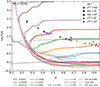 |
Fig. 9. Same as Fig. 8, but for a 50 M⊙ donor star. The symbols indicate possible initial configurations for AB 7. The shapes of the symbols indicate whether we estimated the O-star mass with the mass ratio from radial velocity variations and the WR mass from its luminosity (circle), estimated the mass ratio with the surface-gravity mass of the O star and the luminosity mass of the WR star (squares), with the spectral-type mass of the O star and the luminosity mass of the WR star (diamonds), estimated the WR mass with the mass ratio and the surface-gravity mass of the O star (triangles up), or the mass ratio and the spectral-type mass (triangles down; see also Table 3). |
The case of conservative evolution (blue) places the system into the contact-forming side of the diagram for all five methods. This means that under this assumption, the system must have experienced contact or L2 overflow, which we have argued leads to a merger and not to the stripping of the envelope of the WR progenitor. On the other hand, only initial mass ratios below unity are meaningful. This is fulfilled for all five methods except for the method that is based on the WR mass derived from the mass-luminosity relation and the spectroscopic mass ratio, for which we find initial mass ratios above unity for mass-transfer efficiencies > 25%. All other methods yield initial configurations for the fully non-conservative case (pink) that are on the contact-avoiding side.
A closer inspection of the diagram reveals that for ε > 50% (orange), there are only unrealistic solutions (i.e. qi and Pi values are located in the L2 overflow region), and for ε < 5% (purple), there are only realistic ones (i.e. qi and Pi values located in the contact-avoiding region and qi < 1). For ε = 12% (red), the mass estimate based on the mass-luminosity relation and the surface gravity is in the merger region, and for ε = 25% (green), the estimate with mass-luminosity relation and spectral type as well. This suggests that the mass-transfer efficiency for AB 7 was lower than 50%, maybe as low as 5%. A similar analysis for AB 3 yields ε < 1…5%, for AB 6 ε < 50%, and for AB 8 ε < 25% (Sect. 4).
Other angular momentum budgets give similar results. In general, the ejection of a more specific orbital angular momentum requires a lower mass-transfer efficiency to obtain realistic initial configurations. Furthermore, we find that in almost all scenarios, it was a Case A RLO that formed AB 6, AB 7, and AB 8 (initial configuration below the dashed grey line), while AB 3 was likely formed in Case B. This agrees with the fact that we found it to have the lowest mass-transfer efficiency of the analysed systems because the tides in close binary systems are expected to increase the mass-transfer efficiency (e.g. Sen et al. 2022). All four systems are also stable according to the criterion of Ge et al. (2010, 2015, 2020, initial configurations above the dotted lines). Unfortunately, the discrepancy between the different methods for estimating the stellar masses and the large errors of some of them makes a final judgement difficult. More constraining observations would be desired.
3.3.4. Comparison with previous work
The question under which conditions an RLO will lead to a stripped star and avoid a merger or a common envelope has been addressed by many authors. The classical approach is to compare the mass-radius indices of the donor and the Roche lobe. This is equivalent to asking whether the donor radius shrinks faster or slower under mass loss than its Roche radius. The most recent work on this topic is Ge et al. (2010, 2015, 2020), who calculated mass-radius exponents  for donor stars of all evolutionary phases and also reported critical mass ratios for conservative evolution. From their mass-radius exponents, we derived critical mass ratios for all mass-transfer efficiencies using Eq. (62) of Soberman et al. (1997)3, as suggested by the authors, and we plot them as pink lines in Fig. 7 and as dotted lines in Fig. 8. They indicate that dynamical mass transfer is initiated to their left, probably leading to a merger or common envelope. In most cases, the critical mass ratios lie within the regions in which we predict contact and L2 overflow to occur. Dynamical mass transfer only affects contact-avoiding systems with low accretion efficiencies or with high donor-mass systems and short orbital periods. This means that our criterion, the swelling of the accretor and subsequent contact and L2 overflow, is often stronger in deciding for or against a stable RLO. Still, both criteria need to be checked.
Wellstein et al. (2001) approached the occurrence of contact systems by computing a small grid of detailed binary models assuming conservative mass transfer. They distinguished three contact-formation mechanisms. Their q-contact (contact due to higher mass-transfer rates and/or longer thermal timescales of the secondary) is similar to what we observe in our grid. We cannot model what Wellstein et al. (2001) called delayed contact, that is, an initially stable mass transfer that becomes unstable during the widening of the orbit since the mass-radius exponent of the mass donor increases, because our mass-transfer rate is not resolved in time. However, we observe in our models that in close and very unequal systems, the secondary reaches its maximum radius at lower mass (MR = Rmax = mM2i) than in wide and more equal systems. Finally, no premature and reverse contact occurs in our study because we did not assume nuclear evolution of the secondary. We compared Fig. 12 of Wellstein et al. (2001) with our Fig. 8 (top, conservative case). While they are qualitatively similar, Wellstein et al. (2001) have a larger Case B region with contact avoidance and a smaller corresponding region with Case A region. The reason might be that although fast Case A and Case B take place on a thermal timescale, this is only the order of magnitude. Their duration in detailed binary models differs by a factor of a few. In agreement with them, we find that the contact avoidance regions shrink and the dominance of Case A increases with mass.
Langer et al. (2020), Wang et al. (2020), and Sen et al. (2022) used an energy criterion to determine the stability of the RLO. When the combined luminosity of the two stars is high enough to unbind the unaccreted material from the system, a merger is avoided. They determined the amount of accretion by allowing the accretor to accrete until it reached critical rotation. This led to accretion efficiencies lower than 5% for a Case B mass transfer and up to 50% for in Case A (Sen et al. 2022). Although these detailed models were able to indicate a merger by an L2 overflow, their accretion efficiencies are so low that L2 overflows only occurs at very short initial orbital periods. The energy criterion, however, predicts that many more systems undergo unstable RLO, which covers all the unstable models according to our criterion. Thus, it is in general the energy criterion that decides for or against a stable RLO. We compared our Fig. 8 with Fig. A.4 (right) and A.9 (right) of Wang (2022) because they used the same donor mass, metallicity, and angular momentum budget. While for the 10 M⊙ models Wang (2022) reported that the region of stable mass transfer had a triangular shape between 5 and 100 d up to a mass ratio of about 0.65 and a few Case A systems up to a mass ratio of 0.8 to avoid contact (see also Fig. B.1 in Langer et al. 2020), we find a much larger area when the accretion efficiency is below 50%. Our shape of the contact-avoiding regions is also very different, especially since we find one but Wang (2022) find two separate regions. Its upper limit is given by the onset of convection in the donor. To allow the same number of systems to survive, we would have to set the mass-transfer efficiency to about 100%, which would be centred on systems with close orbits, however. Comparing the 30 M⊙ models, we see that our contact-avoiding regions have shrunk, but in Wang (2022), they have increased by a large amount. Almost all Case B systems and half of the Case A systems avoid contact. To allow the same number of systems to survive, we would have to set our mass-transfer efficiency to about 5%.
Schneider et al. (2015) used fixed critical-mass ratios for Cases A and B to decide as the merger criterion, but limited the accretion by the thermal timescale of the accretor (Hurley et al. 2002). In the language of our work, ε = 1 if t < 1, and when t is greater than 1, ε is adjusted so that t = 1. For a 10 M⊙ donor, this leads to Fig. 1 of Schneider et al. (2015), where Case A yields a stripped donor star for mass ratios greater than 0.56, which is similar to our work, but their Case B is split into a conservative case for high mass ratios and short orbital periods, and a highly non-conservative case otherwise. The line between these cases roughly corresponds to our line between contact and contact avoidance, but it differs because our tmax is mass-dependent and we let the accretor swell. For higher donor masses, Schneider et al. (2015) reported that the region of conservative mass transfer shrinks slightly (as does our contact-avoidance region), but the dividing line becomes an extended transition region (their 20 M⊙ models in Fig. 19).
Henneco et al. (2024) analysed which initial binary configurations led to a merger or common-envelope evolution by calculating detailed binary models up to 20 M⊙. Since rotation-limited accretion was assumed, their mass-transfer efficiency was about 50% for Case A and about 15% for Case B mass transfer. Thus, in agreement with our work, they found that Case A systems with low initial mass ratios evolved towards a merger due to the swelling of the accretor. Because of the low mass-transfer efficiency in their models, it is likely that the evolution of the mass-radius exponents of the donor stars rather than the accretor swelling leads to contact in their Case B systems with extreme initial mass ratios. They also found Case A systems at initial mass ratios close to unity as merger candidates, which we do not find because we did not model the nuclear evolution of the accretor.
Lau et al. (2024) assumed that the formation of contact leads to non-conservative mass transfer, which may cause a merger when the ejected material carries a high enough specific angular momentum, while we assumed this in the first place. Similar to our results about WR stars, they found that in high-mass X-ray binaries and gravitational-wave sources, a non-conservative mass transfer is likely.
4. Conclusion and outlook
Our work sheds new light on the question in which part of the initial binary parameter space the merging of the two stars can be avoided during their first mass-transfer phase. When a fixed mass-transfer efficiency is assumed, the answer to this question depends on the swelling of the mass-accreting star and on the evolution of the orbital separation during the mass transfer. The former can be well computed by detailed binary evolution models, for which it is difficult to scan through the rather unconstrained accretion and angular momentum loss efficiencies, however. Therefore, we developed a theoretical framework in which we first derived analytic approximations for the radius evolution of accreting main-sequence stars based on detailed models (Eqs. (7) and (8)), which we then used to predict the part of the initial binary parameter space in which merging can be avoided as a function of the chosen accretion efficiency and angular momentum loss parameter.
We derived regions in the plane of the initial mass ratio to initial orbital period in which the binary models evolve into L2 overflow, potentially leading to a merger, and the regions in which the binaries avoid contact and develop a fully stripped donor with a main-sequence companion. We find that only very few models evolve into contact and avoid L2 overflow. We tested and compared our binary evolution approach with detailed binary evolution models, for which we find reasonable agreement, but we find rather significant differences compared to the simple merger criteria that were often used in rapid binary evolution calculations. Our models predict a larger fraction of binaries to merge than most previous studies, even at the low metallicity of the SMC. For higher metallicities, we expect the mass gainers to swell more, which would result in more mergers.
We applied our results to interpret the observations of the WR+O stars observed in the SMC. We found that the mass-transfer process that has produced these binaries must have been inefficient, with a mass-transfer efficiency of 50% or lower, and as low as 1% for one particular system.
We developed a fast and powerful method for determining the outcome of a RLO, which often provides stronger constraints than the classical approach of comparing mass-radius exponents. We found that while the angular momentum loss parameter is important, the mass-transfer efficiency is the more influential parameter. Our approach is suitable to be used in rapid population synthesis calculations, for which it is possible to avoid several of the simplifications made here, in particular, neglecting the nuclear evolution of the mass gainer. In a forthcoming paper, we will use our recipe in a rapid binary population synthesis of the population of massive stars after mass transfer in the SMC.
Data availability
We provide further HRDs of accreting main-sequence models (such as Fig. 1) for different initial masses, diagrams showing the boundary between the contact-developing and the contact-avoiding models for other angular momentum budgets than in Fig. 8, and analysis plots for all SMC WR stars (such as Fig. 9) online at https://zenodo.org/records/13384141.
Acknowledgments
The authors would like to thank Pablo Marchant for allowing us to use his MESA framework, and the members of the Bonn Stellar Physics Group for the fruitful discussions.
References
- Bartzakos, P., Moffat, A. F. J., & Niemela, V. S. 2001, MNRAS, 324, 33 [NASA ADS] [CrossRef] [Google Scholar]
- Belczynski, K., Kalogera, V., & Bulik, T. 2002, ApJ, 572, 407 [NASA ADS] [CrossRef] [Google Scholar]
- Belczynski, K., Kalogera, V., Rasio, F. A., et al. 2008, ApJS, 174, 223 [Google Scholar]
- Bodensteiner, J., Shenar, T., Mahy, L., et al. 2020, A&A, 641, A43 [NASA ADS] [CrossRef] [EDP Sciences] [Google Scholar]
- Brott, I., de Mink, S. E., Cantiello, M., et al. 2011, A&A, 530, A115 [NASA ADS] [CrossRef] [EDP Sciences] [Google Scholar]
- Cantiello, M., & Langer, N. 2010, A&A, 521, A9 [NASA ADS] [CrossRef] [EDP Sciences] [Google Scholar]
- Choi, J., Dotter, A., Conroy, C., et al. 2016, ApJ, 823, 102 [Google Scholar]
- Davis, P. J., Siess, L., & Deschamps, R. 2013, A&A, 556, A4 [NASA ADS] [CrossRef] [EDP Sciences] [Google Scholar]
- de Mink, S. E., Pols, O. R., & Hilditch, R. W. 2007, A&A, 467, 1181 [NASA ADS] [CrossRef] [EDP Sciences] [Google Scholar]
- de Mink, S. E., Cantiello, M., Langer, N., et al. 2009a, A&A, 497, 243 [NASA ADS] [CrossRef] [EDP Sciences] [Google Scholar]
- de Mink, S. E., Pols, O. R., Langer, N., & Izzard, R. G. 2009b, A&A, 507, L1 [NASA ADS] [CrossRef] [EDP Sciences] [Google Scholar]
- de Mink, S. E., Langer, N., Izzard, R. G., Sana, H., & de Koter, A. 2013, ApJ, 764, 166 [Google Scholar]
- Deschamps, R., Siess, L., Davis, P. J., & Jorissen, A. 2013, A&A, 557, A40 [NASA ADS] [CrossRef] [EDP Sciences] [Google Scholar]
- Dufton, P. L., Langer, N., Dunstall, P. R., et al. 2013, A&A, 550, A109 [NASA ADS] [CrossRef] [EDP Sciences] [Google Scholar]
- Eggleton, P. P. 1971, MNRAS, 151, 351 [CrossRef] [Google Scholar]
- Eggleton, P. P. 1972, MNRAS, 156, 361 [NASA ADS] [Google Scholar]
- Eggleton, P. P. 1973, MNRAS, 163, 279 [CrossRef] [Google Scholar]
- Eggleton, P. P. 1983, ApJ, 268, 368 [Google Scholar]
- Eggleton, P. P., Faulkner, J., & Flannery, B. P. 1973, A&A, 23, 325 [NASA ADS] [Google Scholar]
- Flannery, B. P., & Ulrich, R. K. 1977, ApJ, 212, 533 [NASA ADS] [CrossRef] [Google Scholar]
- Foellmi, C. 2004, A&A, 416, 291 [NASA ADS] [CrossRef] [EDP Sciences] [Google Scholar]
- Foellmi, C., Moffat, A. F. J., & Guerrero, M. A. 2003, MNRAS, 338, 360 [NASA ADS] [CrossRef] [Google Scholar]
- Fujimoto, M. Y., & Iben, Jr., I. 1989, ApJ, 341, 306 [NASA ADS] [CrossRef] [Google Scholar]
- Gagnier, D., Rieutord, M., Charbonnel, C., Putigny, B., & Espinosa Lara, F. 2019, A&A, 625, A88 [NASA ADS] [CrossRef] [EDP Sciences] [Google Scholar]
- Ge, H., Hjellming, M. S., Webbink, R. F., Chen, X., & Han, Z. 2010, ApJ, 717, 724 [NASA ADS] [CrossRef] [Google Scholar]
- Ge, H., Webbink, R. F., Chen, X., & Han, Z. 2015, ApJ, 812, 40 [Google Scholar]
- Ge, H., Webbink, R. F., Chen, X., & Han, Z. 2020, ApJ, 899, 132 [NASA ADS] [CrossRef] [Google Scholar]
- Gräfener, G., Vink, J. S., de Koter, A., & Langer, N. 2011, A&A, 535, A56 [NASA ADS] [CrossRef] [EDP Sciences] [Google Scholar]
- Hansen, C. J., Kawaler, S. D., & Trimble, V. 2004, Stellar interiors : physical principles, structure and evolution (New York: Springer-Verlag) [CrossRef] [Google Scholar]
- Hastings, B., Langer, N., Wang, C., Schootemeijer, A., & Milone, A. P. 2021, A&A, 653, A144 [NASA ADS] [CrossRef] [EDP Sciences] [Google Scholar]
- Heger, A., Langer, N., & Woosley, S. E. 2000, ApJ, 528, 368 [NASA ADS] [CrossRef] [Google Scholar]
- Henneco, J., Schneider, F. R. N., & Laplace, E. 2024, A&A, 682, A169 [NASA ADS] [CrossRef] [EDP Sciences] [Google Scholar]
- Hjellming, M. S. 1989a, Space Sci. Rev., 50, 155 [NASA ADS] [CrossRef] [Google Scholar]
- Hjellming, M. S. 1989b, Ph.D. Thesis, University of Illinois, Urbana-Champaign, USA [Google Scholar]
- Hjellming, M. S., & Webbink, R. F. 1987, ApJ, 318, 794 [Google Scholar]
- Hurley, J. R., Tout, C. A., & Pols, O. R. 2002, MNRAS, 329, 897 [Google Scholar]
- Iglesias, C. A., & Rogers, F. J. 1996, ApJ, 464, 943 [NASA ADS] [CrossRef] [Google Scholar]
- Ivanova, N., Justham, S., Chen, X., et al. 2013, A&ARv, 21, 59 [Google Scholar]
- Kippenhahn, R., & Meyer-Hofmeister, E. 1977, A&A, 54, 539 [NASA ADS] [Google Scholar]
- Kippenhahn, R., & Weigert, A. 1967, Z. Astrophys., 65, 251 [NASA ADS] [Google Scholar]
- Kippenhahn, R., Weigert, A., & Weiss, A. 2013, Stellar Structure and Evolution [Google Scholar]
- Klencki, J., Nelemans, G., Istrate, A. G., & Pols, O. 2020, A&A, 638, A55 [NASA ADS] [CrossRef] [EDP Sciences] [Google Scholar]
- Klencki, J., Istrate, A., Nelemans, G., & Pols, O. 2022, A&A, 662, A56 [NASA ADS] [CrossRef] [EDP Sciences] [Google Scholar]
- Kruckow, M. U., Tauris, T. M., Langer, N., et al. 2016, A&A, 596, A58 [NASA ADS] [CrossRef] [EDP Sciences] [Google Scholar]
- Kruckow, M. U., Tauris, T. M., Langer, N., Kramer, M., & Izzard, R. G. 2018, MNRAS, 481, 1908 [CrossRef] [Google Scholar]
- Langer, N. 1989, A&A, 210, 93 [NASA ADS] [Google Scholar]
- Langer, N. 2012, ARA&A, 50, 107 [CrossRef] [Google Scholar]
- Langer, N., Schürmann, C., Stoll, K., et al. 2020, A&A, 638, A39 [NASA ADS] [CrossRef] [EDP Sciences] [Google Scholar]
- Lau, M. Y. M., Hirai, R., Mandel, I., & Tout, C. A. 2024, ApJ, 966, L7 [NASA ADS] [CrossRef] [Google Scholar]
- Maeder, A., & Meynet, G. 2000, ARA&A, 38, 143 [Google Scholar]
- Marchant, P. 2017, Ph.D. Thesis, Rheinische Friedrich Wilhelms University of Bonn, Germany [Google Scholar]
- Marchant, P., & Bodensteiner, J. 2024, ARA&A, 62, 21 [NASA ADS] [CrossRef] [Google Scholar]
- Margutti, R., & Chornock, R. 2021, ARA&A, 59, 155 [NASA ADS] [CrossRef] [Google Scholar]
- Moe, M., & Di Stefano, R. 2017, ApJS, 230, 15 [Google Scholar]
- Nariai, K., & Sugimoto, D. 1976, PASJ, 28, 593 [NASA ADS] [Google Scholar]
- Neo, S., Miyaji, S., Nomoto, K., & Sugimoto, D. 1977, PASJ, 29, 249 [NASA ADS] [Google Scholar]
- Niemela, V. S., Massey, P., Testor, G., & Giménez Benítez, S. 2002, MNRAS, 333, 347 [NASA ADS] [CrossRef] [Google Scholar]
- Packet, W. 1981, A&A, 102, 17 [NASA ADS] [Google Scholar]
- Packet, W., & De Greve, J. P. 1979, A&A, 75, 255 [NASA ADS] [Google Scholar]
- Palacios, A., Charbonnel, C., Talon, S., & Siess, L. 2006, A&A, 453, 261 [NASA ADS] [CrossRef] [EDP Sciences] [Google Scholar]
- Pauli, D., Langer, N., Aguilera-Dena, D. R., Wang, C., & Marchant, P. 2022, A&A, 667, A58 [NASA ADS] [CrossRef] [EDP Sciences] [Google Scholar]
- Paxton, B., Bildsten, L., Dotter, A., et al. 2011, ApJS, 192, 3 [Google Scholar]
- Paxton, B., Cantiello, M., Arras, P., et al. 2013, ApJS, 208, 4 [Google Scholar]
- Paxton, B., Marchant, P., Schwab, J., et al. 2015, ApJS, 220, 15 [Google Scholar]
- Paxton, B., Schwab, J., Bauer, E. B., et al. 2018, ApJS, 234, 34 [NASA ADS] [CrossRef] [Google Scholar]
- Paxton, B., Smolec, R., Schwab, J., et al. 2019, ApJS, 243, 10 [Google Scholar]
- Perlmutter, S., Aldering, G., Goldhaber, G., et al. 1999, ApJ, 517, 565 [Google Scholar]
- Pols, O. R. 1994, A&A, 290, 119 [Google Scholar]
- Pols, O. R., & Marinus, M. 1994, A&A, 288, 475 [NASA ADS] [Google Scholar]
- Pols, O. R., Cote, J., Waters, L. B. F. M., & Heise, J. 1991, A&A, 241, 419 [NASA ADS] [Google Scholar]
- Portegies Zwart, S. F., & Verbunt, F. 1996, A&A, 309, 179 [NASA ADS] [Google Scholar]
- Riess, A. G., Filippenko, A. V., Challis, P., et al. 1998, AJ, 116, 1009 [Google Scholar]
- Rivinius, T., Carciofi, A. C., & Martayan, C. 2013, A&ARv, 21, 69 [Google Scholar]
- Sana, H., de Mink, S. E., de Koter, A., et al. 2012, Science, 337, 444 [Google Scholar]
- Sanyal, D., Grassitelli, L., Langer, N., & Bestenlehner, J. M. 2015, A&A, 580, A20 [NASA ADS] [CrossRef] [EDP Sciences] [Google Scholar]
- Sanyal, D., Langer, N., Szécsi, D., Yoon, C. S., & Grassitelli, L. 2017, A&A, 597, A71 [NASA ADS] [CrossRef] [EDP Sciences] [Google Scholar]
- Schmidt, B. P., Suntzeff, N. B., Phillips, M. M., et al. 1998, ApJ, 507, 46 [NASA ADS] [CrossRef] [Google Scholar]
- Schneider, F. R. N., Izzard, R. G., Langer, N., & de Mink, S. E. 2015, ApJ, 805, 20 [Google Scholar]
- Schneider, F. R. N., Ohlmann, S. T., Podsiadlowski, P., et al. 2019, Nature, 574, 211 [Google Scholar]
- Schootemeijer, A., & Langer, N. 2018, A&A, 611, A75 [NASA ADS] [CrossRef] [EDP Sciences] [Google Scholar]
- Schootemeijer, A., Langer, N., Grin, N. J., & Wang, C. 2019, A&A, 625, A132 [NASA ADS] [CrossRef] [EDP Sciences] [Google Scholar]
- Schootemeijer, A., Shenar, T., Langer, N., et al. 2024, A&A, 689, A157 [NASA ADS] [CrossRef] [EDP Sciences] [Google Scholar]
- Schürmann, C., Langer, N., Kramer, J. A., et al. 2024, A&A, 690, A282 [NASA ADS] [CrossRef] [EDP Sciences] [Google Scholar]
- Sen, K., Langer, N., Marchant, P., et al. 2022, A&A, 659, A98 [NASA ADS] [CrossRef] [EDP Sciences] [Google Scholar]
- Shao, Y., & Li, X.-D. 2014, ApJ, 796, 37 [Google Scholar]
- Shao, Y., & Li, X.-D. 2016, ApJ, 833, 108 [NASA ADS] [CrossRef] [Google Scholar]
- Shaviv, G., & Starrfield, S. 1988, ApJ, 335, 383 [NASA ADS] [CrossRef] [Google Scholar]
- Shenar, T., Hainich, R., Todt, H., et al. 2016, A&A, 591, A22 [NASA ADS] [CrossRef] [EDP Sciences] [Google Scholar]
- Shenar, T., Hainich, R., Todt, H., et al. 2018, A&A, 616, A103 [NASA ADS] [CrossRef] [EDP Sciences] [Google Scholar]
- Shenar, T., Bodensteiner, J., Abdul-Masih, M., et al. 2020a, A&A, 639, L6 [EDP Sciences] [Google Scholar]
- Shenar, T., Gilkis, A., Vink, J. S., Sana, H., & Sander, A. A. C. 2020b, A&A, 634, A79 [NASA ADS] [CrossRef] [EDP Sciences] [Google Scholar]
- Siess, L. 2006, A&A, 448, 717 [NASA ADS] [CrossRef] [EDP Sciences] [Google Scholar]
- Siess, L., & Arnould, M. 2008, A&A, 489, 395 [NASA ADS] [CrossRef] [EDP Sciences] [Google Scholar]
- Siess, L., Dufour, E., & Forestini, M. 2000, A&A, 358, 593 [Google Scholar]
- Siess, L., Izzard, R. G., Davis, P. J., & Deschamps, R. 2013, A&A, 550, A100 [NASA ADS] [CrossRef] [EDP Sciences] [Google Scholar]
- Soberman, G. E., Phinney, E. S., & van den Heuvel, E. P. J. 1997, A&A, 327, 620 [NASA ADS] [Google Scholar]
- Steinacker, A., & Papaloizou, J. C. B. 2002, ApJ, 571, 413 [NASA ADS] [CrossRef] [Google Scholar]
- St-Louis, N., Moffat, A. F. J., Marchenko, S., & Pittard, J. M. 2005, ApJ, 628, 953 [NASA ADS] [CrossRef] [Google Scholar]
- Tauris, T. M., & van den Heuvel, E. P. J. 2006, Compact stellar X-ray sources, 39, 623 [NASA ADS] [CrossRef] [Google Scholar]
- Tauris, T. M., & van den Heuvel, E. P. J. 2023, Physics of Binary Star Evolution. From Stars to X-ray Binaries and Gravitational Wave Sources [Google Scholar]
- Toonen, S., Nelemans, G., & Portegies Zwart, S. 2012, A&A, 546, A70 [NASA ADS] [CrossRef] [EDP Sciences] [Google Scholar]
- Ulrich, R. K., & Burger, H. L. 1976, ApJ, 206, 509 [NASA ADS] [CrossRef] [Google Scholar]
- van Son, L. A. C., de Mink, S. E., Callister, T., et al. 2022, ApJ, 931, 17 [NASA ADS] [CrossRef] [Google Scholar]
- Vanbeveren, D., De Donder, E., Van Bever, J., Van Rensbergen, W., & De Loore, C. 1998, New Astron., 3, 443 [CrossRef] [Google Scholar]
- Vigna-Gómez, A., Neijssel, C. J., Stevenson, S., et al. 2018, MNRAS, 481, 4009 [Google Scholar]
- Wang, C. 2022, Ph.D. Thesis, Rheinische Friedrich-Wilhelms-Universität Bonn, Germany [Google Scholar]
- Wang, C., Langer, N., Schootemeijer, A., et al. 2020, ApJ, 888, L12 [NASA ADS] [CrossRef] [Google Scholar]
- Webbink, R. F. 1985, in Interacting Binary Stars, eds. J. E. Pringle, & R. A. Wade, 39 [Google Scholar]
- Wellstein, S., Langer, N., & Braun, H. 2001, A&A, 369, 939 [NASA ADS] [CrossRef] [EDP Sciences] [Google Scholar]
- Yoon, S. C., Langer, N., & Norman, C. 2006, A&A, 460, 199 [NASA ADS] [CrossRef] [EDP Sciences] [Google Scholar]
- Zahn, J. P. 1977, A&A, 57, 383 [Google Scholar]
- Zhao, Z.-Q., Li, Z.-W., Xiao, L., Ge, H.-W., & Han, Z.-W. 2024, MNRAS, 531, L45 [NASA ADS] [CrossRef] [Google Scholar]
All Tables
All Figures
|
Fig. 1. Evolution of our accreting single-star models. Top: Evolution of the 5 M⊙ models in the HRD for different accretion rates (indicated by colour). Stably swelling models are shown with solid lines, and unstable models are plotted with dashed lines. We also show the ZAMS (black) and various lines of a constant radius (grey). Bottom: Radius of accreting models as a function of mass until they reach maximum radius. For each initial mass, the colours are the same as in the corresponding HRDs (top panel and Sect. 4). Models that become unstable are indicated by dashed lines. Some are so short that they are hardly visible. The ZAMS radius is shown in black. |
| In the text | |
|
Fig. 2. Initial mass and adopted accretion rate for our stable (green) and unstable (red) models. Not all models are shown because we focus on the boundary between stable and unstable models at high masses. The blue lines indicate the Eddington accretion rate assuming electron-scattering opacity. |
| In the text | |
|
Fig. 3. Maximum radius of accreting models as a function of initial mass and ratio of the thermal and mass-transfer timescales. Unstable models are shown in red. Special symbols are used for selected accretion rates. The two black lines distinguish between stable and unstable models. |
| In the text | |
|
Fig. 4. Logarithmic radius increase r of accreting models as a function of initial mass and ratio of the thermal and mass-transfer timescale together with our fit (lines) for selected initial masses (top) and for selected timescale ratios (bottom). |
| In the text | |
|
Fig. 5. Mass at which accreting models reach their largest radius as a function of initial mass and ratio of the thermal and mass-transfer timescale together with our fit for selected initial masses (top) and for selected timescale ratios (bottom). |
| In the text | |
|
Fig. 6. Mass-radius evolution (solid line) of detailed accretor models for different initial periods (colour) and initial accretor masses (top 4 M⊙, middle 6 M⊙, bottom 8 M⊙). The donor always has an initial mass of 10 M⊙. The size of the accretor Roche lobe and L2 sphere are shown as dashed and dotted lines. We used crosses to indicate the maximum of the mass-radius curve (Rmax, MR = Rmax) according to Eqs. (7) and (8), based on the maximum mass-transfer rate of the detailed model. The plusses indicate the same, but for an estimate of the mass-transfer rate based on the conditions just before the RLO (Eq. (9)). When a symbol is placed at a high radius but at the initial mass of the model, the model is expected to swell unstably, and the radius is the Hayashi radius (see Sect. 3.1). |
| In the text | |
|
Fig. 7. Maximum ratio of the accretor radius to its Roche radius over the course of the RLO as a function of initial mass and initial orbital period in our simulated binary systems. Red means that the accretor star swells to become larger than its Roche lobe, and blue indicates that it remains within its Roche lobe. The black line marks the boundary between these, and in grey, we show the boundary for the L2 radius instead of the Roche radius. The dotted black and grey lines indicate a shift of ±0.5 dex in the two boundaries. The initial donor masses are 10 M⊙ (top) and 30 M⊙ (bottom), the mass-transfer efficiency is 50%, and we assume that the ejected material carries the specific orbital angular momentum of the accretor (α = η = 0, β = −ε, B = 1). We show the region in which RLO at ZAMS is expected (solid cyan line), the boundary between Case A and Case B (dashed green line), the onset of the donor convective envelope (dot-dashed orange line), and the critical mass ratio according to Ge et al. (2010, 2015, 2020), pink dotted line). Systems marked with numbers and black symbols are those for which we computed detailed models (see Table 2). The black circles indicate stable swelling without contact formation, squares stand for stable swelling but L2 overflow, and diamonds indicate unstable swelling with L2 overflow. |
| In the text | |
|
Fig. 8. Boundary between the contact-developing and the contact-avoiding models for different initial donor masses (from top to bottom, 10, 30, and 100 M⊙) assuming the ejected material carries the specific orbital angular momentum of the accretor (i.e. α = η = 0, β = −ε, B = 1). The colours indicate the assumed mass-transfer efficiency. The dashed lines show the boundary of L2 overflow, and the dotted lines represent the critical mass ratio for dynamical timescale mass transfer derived from Ge et al. (2010, 2015, 2020). |
| In the text | |
|
Fig. 9. Same as Fig. 8, but for a 50 M⊙ donor star. The symbols indicate possible initial configurations for AB 7. The shapes of the symbols indicate whether we estimated the O-star mass with the mass ratio from radial velocity variations and the WR mass from its luminosity (circle), estimated the mass ratio with the surface-gravity mass of the O star and the luminosity mass of the WR star (squares), with the spectral-type mass of the O star and the luminosity mass of the WR star (diamonds), estimated the WR mass with the mass ratio and the surface-gravity mass of the O star (triangles up), or the mass ratio and the spectral-type mass (triangles down; see also Table 3). |
| In the text | |
Current usage metrics show cumulative count of Article Views (full-text article views including HTML views, PDF and ePub downloads, according to the available data) and Abstracts Views on Vision4Press platform.
Data correspond to usage on the plateform after 2015. The current usage metrics is available 48-96 hours after online publication and is updated daily on week days.
Initial download of the metrics may take a while.