| Issue |
A&A
Volume 689, September 2024
|
|
|---|---|---|
| Article Number | A263 | |
| Number of page(s) | 16 | |
| Section | Extragalactic astronomy | |
| DOI | https://doi.org/10.1051/0004-6361/202449875 | |
| Published online | 20 September 2024 | |
GATOS: missing molecular gas in the outflow of NGC 5728 revealed by JWST
1
Max Planck Institute for Extraterrestrial Physics (MPE), Giessenbachstr.1, 85748 Garching, Germany
2
Instituto de Física Fundamental, CSIC, Calle Serrano 123, 28006 Madrid, Spain
3
Centro de Astrobiología (CSIC-INTA), Camino Bajo del Castillo s/n, 28692 Villanueva de la Cañada, Madrid, Spain
4
Instituto de Astrofísica de Canarias, Calle Vía Láctea, s/n, 38205 La Laguna, Tenerife, Spain
5
Departamento de Astrofísica, Universidad de La Laguna, 38205 La Laguna, Tenerife, Spain
6
Departmento de Física de la Tierra y Astrofísica, Fac. de CC Físicas, Universidad Complutense de Madrid, 28040 Madrid, Spain
7
Instituto de Física de Partículas y del Cosmos IPARCOS, Fac. CC Físicas, Universidad Complutense de Madrid, 28040 Madrid, Spain
8
Cahill Center for Astronomy and Astrophysics, California Institute of Technology, Pasadena, CA 91125, USA
9
School of Mathematics, Statistics and Physics, Newcastle University, Newcastle upon Tyne NE1 7RU, UK
10
LERMA, Observatoire de Paris, Collège de France, PSL University, CNRS, Sorbonne University, Paris
11
Department of Physics & Astronomy, University of Alaska Anchorage, Anchorage, AK 99508-4664, USA
12
Institute of Astrophysics, Foundation for Research and Technology-Hellas, Heraklion 70013, Greece
13
School of Sciences, European University Cyprus, Diogenes street, Engomi, 1516 Nicosia, Cyprus
14
Department of Physics and Astronomy, The University of Texas at San Antonio, 1 UTSA Circle, San Antonio, TX 78249, USA
15
Department of Physics & Astronomy, University of Southampton, Hampshire, SO17 1BJ Southampton, UK
16
Department of Physics, University of Oxford, Denys Wilkinson Building, Keble Road, Oxford OX1 3RH, UK
17
Observatorio Astronómico Nacional (OAN-IGN)-Observatorio de Madrid, Alfonso XII, 3, 28014 Madrid, Spain
18
Instituto de Radioastronomía y Astrofísica (IRyA), Universidad Nacional Autónoma de México, Antigua Carretera a Pátzcuaro #8701, ExHda. San José de la Huerta, Morelia, Michoacán C.P. 58089, México
19
National Astronomical Observatory of Japan, National Institutes of Natural Sciences, 2-21-1 Osawa, Mitaka, Tokyo 181-8588, Japan
20
Department of Astronomy, School of Science, Graduate University for Advanced Studies (SOKENDAI), Mitaka, Tokyo 181-8588, Japan
21
Telespazio UK for the European Space Agency, ESAC, Camino Bajo del Castillo s/n, 28692 Villanueva de la Cañada, Spain
22
Space Telescope Science Institute, 3700 San Martin Drive, Baltimore, MD 21218, USA
23
Kavli Institute for Particle Astrophysics & Cosmology (KIPAC), Stanford University, Stanford, CA 94305, USA
24
Núcleo de Astronomía de la Facultad de Ingeniería, Universidad Diego Portales, Av. Ejército Libertador 441, Santiago, Chile
25
Kavli Institute for Astronomy and Astrophysics, Peking University, Beijing 100871, PR China
26
LESIA, Observatoire de Paris, Université PSL, CNRS, Sorbonne Université, Sorbonne Paris Citeé, 5 place Jules Janssen, 92195 Meudon, France
27
Astronomical Observatory, Volgina 7, 11060 Belgrade, Serbia
28
Sterrenkundig Observatorium, Universiteit Gent, Krijgslaan 281-S9, Gent 9000, Belgium
29
School of Physics and Astronomy, Tel Aviv University, Ramat Aviv 69978, Israel
30
Center for Computational Astrophysics, Flatiron Institute, 162 5th Ave, New York, NY 10010, USA
31
Centro de Astrobiología (CAB), CSIC-INTA, Ctra. de Ajalvir, km 4, 28850 Torrejón de Ardoz, Madrid, Spain
32
Centre for Extragalactic Astronomy, Department of Physics, Durham University, South Road, Durham DH1 3LE, UK
Received:
6
March
2024
Accepted:
24
June
2024
The ionisation cones of NGC 5728 have a deficit of molecular gas based on millimetre observations of CO (2-1) emission. Although photoionisation from the active nucleus may lead to suppression of this transition, warm molecular gas can still be present. We report the detection of eight mid-infrared rotational H2 lines throughout the central kiloparsec, including the ionisation cones, using integral field spectroscopic observations with JWST/MIRI MRS. The H2 line ratios, characteristic of a power-law temperature distribution, indicate that the gas is warmest where it enters the ionisation cone through disk rotation, suggestive of shock excitation. In the nucleus, where the data can be combined with an additional seven ro-vibrational H2 transitions, we find that moderate velocity (30 km s−1) shocks in dense (105 cm−3) gas, irradiated by an external UV field (G0 = 103), do provide a good match to the full set. The warm molecular gas in the ionisation cone that is traced by the H2 rotational lines has been heated to temperatures > 200 K. Outside of the ionisation cone the molecular gas kinematics are undisturbed. However, within the ionisation cone, the kinematics are substantially perturbed, indicative of a radial flow, but one that is quantitatively different from the ionised lines. We argue that this outflow is in the plane of the disk, implying a short 50 pc acceleration zone up to speeds of about 400 km s−1 followed by an extended deceleration over ∼700 pc where it terminates. The deceleration is due to both the radially increasing galaxy mass, and mass-loading as ambient gas in the disk is swept up.
Key words: galaxies: active / galaxies: individual: NGC 5728 / galaxies: kinematics and dynamics / galaxies: nuclei / galaxies: Seyfert
© The Authors 2024
 Open Access article, published by EDP Sciences, under the terms of the Creative Commons Attribution License (https://creativecommons.org/licenses/by/4.0), which permits unrestricted use, distribution, and reproduction in any medium, provided the original work is properly cited.
This article is published in open access under the Subscribe to Open model.
Open Access funding provided by Max Planck Society.
1. Introduction
It has been known for a number of decades that active galactic nuclei (AGN) drive ionised outflows and that these should play a central role in galaxy evolution (Veilleux et al. 2005; Tombesi et al. 2010; Fabian 2012). The importance of molecular outflows has been realised only more recently (Sturm et al. 2011; Veilleux et al. 2013; Cicone et al. 2014; Fiore et al. 2017; Morganti 2017; Veilleux et al. 2020). There is an ongoing effort to assess outflow rates and kinetic powers in order to understand how efficiently these various outflows couple to the interstellar medium and their impact in terms of the host galaxy gas depletion timescale and star formation rate (Fiore et al. 2017; Rupke et al. 2017; Fluetsch et al. 2019; Lutz et al. 2020; Fluetsch et al. 2021; Lamperti et al. 2022; Ramos Almeida et al. 2022). This is complicated by the inter-dependence of many of the galaxy and AGN properties. These include black hole mass, AGN luminosity, stellar mass, and star formation rate; by the role of geometry, and of the timescales of the processes involved; and by the observational impacts between, for example, type 1 and type 2 AGN, or radiative and mechanical processes. One outcome of the studies of global properties on scales of kilo-parsecs or more, has been the suggestion that many (perhaps most) molecular outflows remove gas only from the central regions and that this will be re-accreted onto the host galaxy, or equivalently that AGN do not remove gas or quench star formation on a global galaxy scale (Rosario et al. 2018; Shangguan et al. 2018, 2020; Fluetsch et al. 2019; Ellison et al. 2021; Ramos Almeida et al. 2022; Lammers et al. 2023; Molina et al. 2023). This points to a need to study these outflows on smaller scales.
Indeed, there has been an extensive parallel effort to attain a more detailed view of the mechanisms at work in the circumnuclear regions, on scales of a few to a few hundred parsecs, to understand how the molecular gas is accelerated. Such studies are inevitably detailed, and so often focus on individual archetypal objects such as NGC 1068 (García-Burillo et al. 2014; Gallimore et al. 2016; Impellizzeri et al. 2019; Imanishi et al. 2020) or outflows associated with a jet as in IC 5063 (Morganti et al. 2015; Oosterloo et al. 2017) and the teacup quasar (Audibert et al. 2023). In a number of cases, the molecular outflow appears to be radial in the plane of the inner disk (Alonso-Herrero et al. 2018, 2019, 2023; Esposito 2024) or the result of an interaction between the ionised outflow and the molecular disk (Davies et al. 2014). It is in this context that we study here the molecular gas influenced by the outflow in NGC 5728, which is a strongly barred disk galaxy at a distance of 39 Mpc. This galaxy hosts an obscured AGN (optical type 2 and X-ray column log NH (cm−2) = 24.2) with a bolometric luminosity log LAGN (erg s−1) = 44.1 (Davies et al. 2015) and, an Eddington ratio ≳0.1 for a black hole mass ≲8 × 10⁶ M⊙ (Kuo et al. 2020). Based on the measurement of σ * = 168 km s−1 in both the 850 nm Ca triplet feature and 2.3 μm CO (2-0) bandhead (Caglar et al. 2020), this puts the AGN well below the MBH − σ* relation.
The disk of NGC 5728 is generally well detected in the CO (2-1) 230.5 GHz line out to radii of 1.5–2 kpc (Shimizu et al. 2019; Shin et al. 2019). It is remarkable, however, that CO emission is not detected in the ionisation cone. Shimizu et al. (2019) suggested that here the AGN photoionisation may lead to suppressed CO (2-1) line emission. This phenomenon has been reported for other objects such as NGC 2110 (Rosario et al. 2019) and ESO 428-G014 (Feruglio et al. 2020), in both of which the molecular gas is revealed by the presence of near-infrared H2 lines tracing the hot component of molecular gas. At smaller scales, different causes for weak CO (3-2) or CO (2-1) emission may be at play. In the central 100 pc of NGC 3227, HCN (1-0) was associated with faint CO (2-1) and explained in terms of high HCN abundance due to X-ray irradiation of the gas by the AGN (Davies et al. 2012). For several objects, in the central few tens of parsecs where there is only faint CO (3-2) emission, the presence of significant molecular gas has been revealed by HCO+ (4-3) and explained in terms of density stratification (García-Burillo et al. 2021). And in Circinus the weak CO (3-2) in the nucleus has been explained in terms of self-absorption, and the presence of molecular gas is revealed via the higher CO (6-5) transition as well as other higher density tracers (Tristram et al. 2022).
For the outflow in NGC 5728 on scales of 100–1000 pc, near-infrared H2 lines have been detected in the outflow, suggesting that molecular gas may be present (Durré & Mould 2018; Shimizu et al. 2019). However, these ro-vibrational lines trace gas at typically 1000–2000 K, which comprises a very small fraction of the total mass. It is therefore expedient to look at the pure rotational H2 lines present at mid-infrared wavelengths, that are produced by warm molecular gas at temperatures of 100–1000 K and which are expected to trace a larger fraction of the total molecular mass. We present an analysis of such observations in this paper.
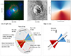 |
Fig. 1. Circumnuclear region of NGC 5728. Top left: three colour montage of the ALMA CO (2-1) map (red), HST F160WH-band continuum (green), and VLT/MUSE [OIII] line emission (blue). These show several key components: the ionisation cone, and the molecular gas that is collimating it, and the direct illumination of the circumnuclear disk by the AGN. Top centre: B-H dust structure map (from F438W and F160W HST images; there is no strong line contamination in these filters) showing the dusty circumnuclear disk to the west and a lighter region to the east where the outflow has removed dust from our line of sight. Top right: velocity field of the disk model fitted to the ALMA CO (2-1) kinematics. Bottom: cartoon showing two views to illustrate the complex geometry, highlighting that the ionisation cone strongly intersects the galaxy disk (similar to scenario A in Ramos Almeida et al. 2022). All panels are adapted from, or based on the kinematic modelling of, Shimizu et al. (2019). The cartoon has been slightly updated to better match the spatial distributions. |
2. The circumnuclear region of NGC 5728
As a context to the study presented here, we summarise the relevant points concerning what is known about the circumnuclear region of NGC 5728. Because it can be well resolved spatially at 100 pc scales or less with 8-m class telescopes at optical and near-infrared wavelengths, it has been studied extensively (Son et al. 2009; Shimizu et al. 2019; Durré & Mould 2018, 2019; Shin et al. 2019). A focus of all these studies has been the prominent star forming ring at a radius of about 800 pc and the ionisation cone, which has also been detected in soft X-rays extending to beyond 1 kpc (Trindade Falcao et al. 2023). These primary features are seen in the top left panel of Fig. 1 and mean that the central kiloparsec of this galaxy is a complex region both morphologically and kinematically.
The top right panel shows a B − H dust structure map, which highlights several key features. Inside the star forming ring, the bright and dark arcs on the western side trace the dusty circumnuclear disk. But the eastern side is very different, dominated by a conical region that is pale, indicating that the dust has been driven out (indeed, this is a typical signature of the interaction of an outflow with the surrounding disk, see for example Davies et al. 2014). While there have been previous suggestions that there may be a circumnuclear stellar bar, based on HST imaging, Wilson et al. (1993) noted that the features could also be scattered nuclear light, which would be more consistent with the dust structure map and also the lack of evidence for a corresponding gaseous bar (Petitpas & Wilson 2002). We propose a cause for the latter interpretation in Sect. 4.2, and argue below that it is also more consistent with the kinematics.
The inflow driven by the large scale bar terminates at its inner Lindblad resonance, at which radius the gas piles up and inevitably forms stars. The kinematics of the disk inside this region are driven by the rotating potential of the bar, which can stimulate a circumnuclear spiral (Maciejewski 2004a, 2004b). As pointed out by Canzian (1993), and shown by Davies et al. (2009) in the context of circumnuclear spirals, an m-arm density perturbation appears as an (m − 1)-arm kinematic wave in the projected line-of-sight velocity field. Thus, when one removes the circular component of the velocity field (e.g. by subtracting a disk model), the projection of the inflow/outflow associated with a 2-arm spiral would appear as a 1-arm kinematic spiral. Indeed, the structure in the residual velocity field for both the molecular gas and the stars does resemble a low amplitude 1-arm spiral (Fig. 9 of Shimizu et al. 2019). We therefore conclude that the kinematics of the disk on scales of about 0.1–1 kpc are consistent with a circumnuclear spiral stimulated by the large scale bar.
There is another structure in the inner 200 pc that is reminiscent of a nuclear bar: a feature in the CO (2-1) map perpendicular to the outflow direction (Figs. 3 and 12 in Shimizu et al. 2019). However, as argued through the decomposition performed in that work and shown through higher resolution data (García-Burillo et al., in prep.), this is in fact a more highly inclined disk on small scales that delineates the plane from which the outflow is emerging. Geometric modelling of the kinematics by Shimizu et al. (2019) indicate that the approaching cone is oriented only 13° behind the near side of the disk, while the receeding cone is 13° in front of the far side of the disk. The modelled opening angle of ±23° means that the cone intersects the disk substantially. This is illustrated in Fig. 1 where we have modified the parameters slightly to better match the spatial distributions, rather than kinematics alone, so that the cone is oriented at a position angle of −60° with an opening angle of ±30°. The inner 200 pc scale disk, because it is closer to edge-on, is likely to be a source of the optical obscuration and X-ray absorbing column that make NGC 5728 a Compton thick Seyfert 2.
The green line in Fig. 1 denotes the direction of the jet that has been reported at both 6 cm and 20 cm, which shows a spectral index typical of synchrotron rather than thermal emission, and which is thought to be interacting with the disk (Schommer et al. 1988; Durré & Mould 2018). The 20 cm image from the NRAO VLA Archive Survey, for which the beam is 2.0″ × 1.2″ at a PA of −2°, highlights that on scales of at least a few hundred parsecs the jet is well aligned with the ionisation cone, and is 1-sided (a reverse jet would have to be at least a factor 10 lower surface brightness at this resolution).
We end this short summary of the circumnuclear region of NGC 5728 with a look at the molecular gas concentration index, or deficit, put forward by García-Burillo et al. (2021). They compared the ratio of molecular mass surface densities within 50 pc (ΣH250 pc) to that at 200 pc (ΣH2200 pc), to the X-ray luminosities. The index log ΣH250 pc/ΣH2200 pc = 0.04 (García-Burillo et al. in prep.) and luminosity of NGC 5728 put it clearly within the locus of AGN which are in the process of removing molecular gas that has built up in their central regions, and so have a flat rather than cuspy radial surface density distribution. This is consistent with its location in the comparison of Eddington ratio to molecular gas column density in Alonso-Herrero et al. (2021). Matching the CO-to-H2 conversion factor used in their analysis, and with the lower limit on Eddington ratio noted above, one finds NGC 5728 in the locus where dusty outflows are expected to be launched. It is important to bear in mind that these comparisons are independent of the detailed morphology, and in particular that the concentration index is comparing gas content on very small scales – within radii of 0.5″ and 2″ for NGC 5728. Thus, the lack of CO (2-1) in the ionisation cones, which is the rationale for the analysis here, is part of the variance between galaxies that the index is designed to minimize; and what the index is tracking is the removal of gas from the inner 200 pc scale edge-on disk introduced above.
3. Sample and target selection
NGC 5728 is one of six galaxies observed in JWST Cycle 1 programme #1670. They form part of the larger sample of AGN in the Galactic Activity, Torus, and Outflow Survey (GATOS1) which are drawn from the 70 Month Swift-BAT All-sky Hard X-ray Survey (Baumgartner et al. 2013). This ensures a nearly complete selection of AGN with luminosities L14 − 150 keV > 1042 erg s−1 at distances of 10–40 Mpc. The selection band also means that the sample is largely unbiased to obscuration/absorption even up to column densities of NH ∼ 1024 cm−2. Both the AGN luminosity and absorbing column are available from the analysis of the X-ray data (Ricci et al. 2017). The GATOS sample, and analysis of the first sub-samples, are described in García-Burillo et al. (2021) and Alonso-Herrero et al. (2021); and a first analysis of the JWST data, focussing on silicate features and water ice at small scales, is presented by García-Bernete et al. (2024). Additional papers about this sample include Zhang et al. (in prep.) giving on overview of the sample, Hermosa Muñoz et al. (in prep.) on NGC 7172, Esparza Arredondo et al. (in prep.) on MCG-05-23-016, Haidar et al. (in prep.) on ESO 137-G034, García-Bernete et al. (in prep.) on the spatially resolved PAHs, and Lopez-Rodriguez et al. (in prep.) on line contamination of continuum images and the dust distribution.
The sub-sample from which NGC 5728 is selected were also part of the Luminous Local AGN and Matched Analogues (LLAMA) survey (Davies et al. 2015) which were drawn from the same parent sample. Observations of these galaxies include integral field spectroscopy at optical and near-infrared wavelengths, the latter using adaptive optics to achieve higher spatial resolution. In particular, they are included in an analysis of the density of ionised outflows (Davies et al. 2020) and so ionised outflow rates calculated in a consistent way are available for all of them. This analysis was only performed for Seyfert types 1.8-2, and so also limits the impact of differing orientations. The sub-sample spans a limited range in distance, stellar mass, and AGN luminosity; but a wide range in ionised outflow rate measured on 150 pc scales. As part of the LLAMA survey, NGC 5728 was the focus of a combined analysis of CO (2-1) data from the Atacama Large Millimeter/submillimeter Array (ALMA) wide field optical integral field spectroscopy from the Very Large telescope (VLT) MUSE and high spatial resolution integral field spectroscopy from VLT/SINFONI (Shimizu et al. 2019). These data are included in the analysis here to supplement the JWST observations.
4. Observations, data processing, map extraction
Observations of NGC 5728 were performed on 13–14 March 2023 using the Medium Resolution Spectrometer (MRS; Wells et al. 2015; Argyriou et al. 2023) of the Mid-infrared Instrument (MIRI; Rieke et al. 2015) on the JWST (Gardner et al. 2023). This instrument offers integral field spectroscopy between 4.9 and 27.9 μm at a resolution of R ∼ 1500 to ∼3500, over a field of view from 3.2″ × 3.9″ at the shortest wavelengths to 6.6″ × 7.7″ at the longest. The full wavelength range comprises 12 segments divided across four channels. To observe the complete range required three sets of observations.
The observations consisted of a 2 × 2 dithered mosaic covering a minimum common field of about 6.6″ × 7.9″ oriented along the direction of the ionised outflow, and covering part of the circumnuclear star-forming ring. There was a single integration of 263 s at each of the four dither positions and for each of the short, medium, and long wavelength settings. The target observations were accompanied by a pair of dithered background exposures, offset by about 2′.
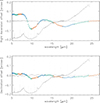 |
Fig. 2. Spectro-astrometry of NGC 5728. The relative position of the continuum peaks are shown for right ascension (top) and declination (bottom). The colours demarcate the spectral channels, showing that the datacubes are well aligned spatially and that there is a wavelength dependent shift of the position. For reference, the equivalent measurement for MCG-05-16-023, dominated by a continuum point source and, as is more typical of the sample, showing no spectro-astrometric shifts is also shown as open diamonds (see Esparza-Arredondo et al. in prep.); and the nuclear spectrum is overplotted. |
4.1. Data reduction
The MIRI MRS data were processed using the JWST Calibration pipeline (version 1.11.4) with the calibration context 1130. We followed the standard MRS pipeline procedure adding some extra steps to correct for bad pixels. We estimated the background emission by calculating the median background level at each wavelength channel in the dedicated background data cubes. This median value for each spectral channel was subtracted from the science data cubes. The data reduction is described in detail in García-Bernete et al. (2022), García-Bernete et al. (2024), and Pereira-Santaella et al. (2022).
In the pipeline data cubes, we found a relatively large offset of 0.27″ in right ascension and 0.06″ in declination between the mid-infrared continuum peak and the 1.3 mm continuum position measured with a 0.5″ beam using ALMA (Shimizu et al. 2019). Therefore, we corrected the astrometry of the 12 individual MIRI MRS datacubes using background galaxies detected in the parallel imaging. After applying this correction, we found that the relative centering precision was about 0.02″ RMS, which could be verified by tracing the peak position of the AGN as a function of wavelength across all the datacubes. The positions at adjacent wavelengths in differing cubes were matched to the same precision.
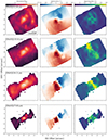 |
Fig. 3. Flux and kinematics maps of four neon lines. The flux (left), velocity (centre), and velocity dispersion (right) of the [Ne II] 12.8 μm, [Ne III] 15.6 μm, [Ne V] 24.3 μm, and [Ne VI] 7.7 μm transitions are shown to provide a context about the circumnuclear region of NGC 5728 (north is up, east is left). As the ionisation potential increases from 22 eV to 126 eV (top to bottom), what the line emission traces changes from star formation in the ring to the outflow. The direction of the major kinematic axis and the central dispersion change correspondingly. Interestingly, the outflow kinematics reveal anomalous velocities and unusually high dispersion along the minor axis, which is especially noticeable in the [Ne III] line. |
4.2. Spectro-astrometric shifts
Interestingly, as shown in Fig. 2, there were significant systematic excursions of the peak position through the cubes, which is in stark contrast to the equivalent measurement in other objects observed with the same set-up such as MGC-05-23-016 which is dominated by a point-like continuum source (Asmus et al. 2014; Esparza-Arredondo et al. in prep.) and the peak position of which shows no measurable shift over the 5–28 μm wavelength range. In NGC 5728 there is a shift of 0.1″ close to the east-west direction centered on the 10 μm silicate absorption feature, and there are secondary shifts of 0.05″ at < 8 μm and around 18 μm. These indicate that the central peak has spatial structure on scales of 0.1″, equivalent to ∼20 pc. The position shifts may be indicative of significant obscuration on those scales as similarly proposed by Díaz-Santos et al. (2011) for ultraluminous infrared galaxies. The scale and direction indicate that it is associated with a sub-structure inside the 200 pc edge-on disk discussed in Sect. 2, perhaps related to the third component identified by Shimizu et al. (2019). It points to another twist of the disk on smaller scales. A similar situation, causing a misalignment between the accretion disk and the outflow direction, has been demonstrated for Circinus (Stalevski et al. 2017, 2019, 2023). In the case of Circinus, it leads to an asymmetric illumination of the dust at the edges of the ionisation cone. Here, the direction of the obscuration gradient implies there is a structure such as a disk with its projected major axis aligned north-south, and tilted a little away from edge-on so that the western side points slightly towards us and is less obscured, while the eastern side is more obscured. This is illustrated as the innermost black line in the cartoon of Fig. 1. Such a geometry would provide a natural explanation for the bar-like brightening in the continuum images: this is instead direct illumination by the accretion disk of the circumnuclear disk at one edge of the ionisation cone. Similar intrinsic anisotropic illumination of the circumnuclear region due to a small scale warped disk was proposed by Tadhunter et al. (2000) for Cygnus A. We leave it as a proposed geometry because the detailed modelling needed to explore the scenario more quantitatively, including how it creates this astrometric signature, and how the sub-pc geometry from the interpretation of the maser measurements as a magnetocentrifugal wind (Kuo et al. 2020) fits in, is beyond the scope of this work.
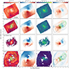 |
Fig. 4. Flux and kinematics maps of molecular lines. The flux (far left), velocity (centre left), velocity dispersion (centre right), and residual velocity after subtracting a disk model (far right) are shown for the H2 0-0 S(1), 0-0 S(3), and 0-0 S(5) and 1.3 mm CO (2-1) lines. The CO data and disk model are from Shimizu et al. (2019). In all cases north is up, east is left. These data are the focus of the analysis in Sect. 5 and Sect. 6. The most striking features are: (i) the morphology and kinematics of the CO and S(1) lines are remarkably similar indicating they trace the same gas component, (ii) while CO is not detected in the ionisation cones, the rotational H2 lines are detected with a perturbed velocity field, and (iii) the largest velocity residuals are well-aligned with the ionisation cone as traced by the [Ne V] emission (black contour) and the radio jet at 20 cm (green contours). |
4.3. Flux and kinematics maps
Flux and kinematics maps for each line were extracted using a single Gaussian fit to the line profile and a linear continuum to match the local continuum. A quadrature correction was applied to the velocity dispersion to account for the instrumental spectral resolution. In order to provide context about the circumnuclear region, the resulting maps for four neon lines are shown in Fig. 3. While these are not a central part of the analysis here, and so are not discussed in detail, we describe the main features that they reveal.
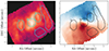 |
Fig. 5. Apertures used for spectral extractions. These are superimposed on the S(5) flux map (left) and velocity field (right). Rather than being circular, they trace specific features within the overlapping fields of view: (1) the star forming arc, (2) an H2 hotspot in the ionisation cone, (3) a knot of H2 emission to the east, (4) the nucleus, and (5) a region to the south outside the ionisation cone. |
The [Ne II] 12.8 μm line with an ionisation potential2 (IP) of 21.6 eV traces star formation in the circumnuclear ring, where the kinematics are dominated by the disk rotation (Shimizu et al. 2019). In the central region, the twist in the zero velocity line indicates that it also traces the outflow. This is much clearer in the [Ne III] 15.6 μm line, which has a higher IP of 41.0 eV and is therefore more influenced by AGN photoionisation. And in both the [Ne V] 24.3 μm and [Ne VI] 7.7 μm lines, with IP of 97.1 eV and 126.2 eV respectively, the emission only has high enough surface brightness to be spatially resolved in the direction of the outflow. In both these lines, the kinematics are completely dominated by the outflow. For the [Ne V] line, the high dispersion oriented perpendicular to the outflow direction is likely to be a beam smearing effect due to the broader PSF (∼0.9″ FWHM) and the rapid change from highly red shifted to highly blue shifted velocities. This effect is not so prominent in the [Ne VI] line where the PSF has a FWHM of ∼0.4″. A different feature that is very clear in the kinematics maps of the [Ne III] line is the anomalous velocity and high dispersion extending from the nucleus along the minor axis out to 2–3″ where the surface brightness of the line emission is much lower. Such features have been reported for other galaxies (Venturi et al. 2021; Peralta de Arriba et al. 2023; Audibert et al. 2023), where the explanation is based on models of young jets in disks (Mukherjee et al. 2018; Meenakshi et al. 2022). This is understood to be lateral turbulence caused by a jet that is inclined towards the host galaxy disk. As it is decelerated and deflected by clouds in the disk, it drives a sub-relativistic wide-angled outflow normal to the disk plane. The shocks caused by this jet-driven bubble increase the velocity dispersion of gas in directions away from the jet itself. It has been identified in a number of other galaxies in our full sample as described in Zhang et al. (in prep.).
Maps of the flux and kinematics extracted for several H2 lines are shown in Fig. 4. In addition to the velocity and velocity dispersion, the figure shows the residual velocity after subtracting the velocity field of the disk model fitted to the CO (2-1) kinematics in Shimizu et al. (2019). These data are analysed in detail in the following sections, and so here we note only the most striking features. The first of these is that the morphology and kinematics of the CO and S(1) lines are remarkably similar indicating they trace the same molecular gas component. The second is that, while CO is not detected in the ionisation cones, the rotational H2 lines are detected. This confirms that molecular gas can survive in the outflow. The velocity field and its residual show that the molecular gas in the disk is perturbed as it passes through the outflow, an effect that is more prominent in the higher excitation molecular lines. It is these features that motivate the analysis of the H2 excitation and temperature distribution in Sect. 5 and of the H2 kinematics in Sect. 6.
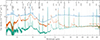 |
Fig. 6. Mid-infrared spectra in NGC 5728. The spectra for three apertures, corresponding to the nucleus (blue; region 4 in Fig. 5), star forming arc (red; region 1 in Fig. 5), and hotspot (green; region 2 in Fig. 5) are shown on a logarithmic flux scale. The spectra have been extracted from each of the 12 separate datacubes and overplotted. They show that no re-scaling between the cubes is needed. The most prominent lines with reliable identifications have been marked: 36 fine structure lines, 3 H I lines, and 8 H2 lines. |
5. Molecular gas excitation and temperature distribution
The MRS bandpass covers the rotational H2 transitions from 0-0 S(8) at 5.05 μm to 0-0 S(1) at 17.04 μm (the 0-0 S(0) line is outside the currently available wavelength range). These have excitation temperatures down to 1015 K and are able to probe molecular gas as cool as ∼100 K, making them an ideal complement to the transitions accessible to millimetre interferometers that tend to probe the coldest component of the gas. In addition, observing eight transitions makes it possible to assess the spatially resolved temperature distribution of the gas. In order to mitigate the impact of the variation in spatial resolution over the wide wavelength range, after resampling the individual cubes to a common pixel grid of 0.13″ (corresponding to the smallest pixel scale of the full data set), we extracted line fluxes in apertures with a minimum width of 0.8″ and mostly > 1″. Tests indicate that in this case PSF effects have no more than a 20% impact on extracted fluxes from S(1) to S(8). This upper limit to the systematic error matches the 20% statistical uncertainty that we consider sufficient for distinguishing models of the H2 population distribution at a meaningful level. We note that it would be incorrect to apply a PSF correction because of the extended nature of the spatial distributions of the lines. The apertures, which have areas in the range 1.7–5.0 sq. arcsec, are irregular in shape because they trace specific features on the emission line maps that characterise the different environments in the field of view. As shown in Fig. 5, these correspond to (1) the star-forming arc, (2) a hotspot in the ionisation cone to the north-west of the nucleus (P5 in Durré & Mould 2018), (3) a knot of emission to the east of the nucleus, (4) the nucleus itself (P1 in Durré & Mould 2018), and (5) a region to the south that is outside the ionisation cone. The spectra extracted in three of the apertures are shown in Fig. 6, and the H2 line fluxes for all five apertures are reported in Table 1.
The analysis we perform in this Section encompasses several aspects, and so we provide a brief summary here before going into the details.
We first look at the populations of the J = 3–10 levels in all the apertures. These show two distinct groupings, hinting at minimum temperatures of 300-400 K for the J = 3–5 levels; but clear evidence for warmer gas that dominates the higher-J transitions. We make simple models of these distributions assuming local thermal equilibrium (LTE) in order to assess the temperature distribution in the different regions. The ortho-para ratio in the LTE models provides a good match to the data, indicating that such models are appropriate for the pure rotational levels (although we find later that the vibrational levels show evidence for an ortho-para ratio < 3, indicating they are modified by non-thermal excitation).
Based on these results, we create an excitation map by looking at the ratio of the S(1) and S(5) lines, since the corresponding J = 3 and J = 7 levels are dominated by cooler and warmer gas respectively. This provides more insights into the spatial distribution, in particular with respect to the boundaries of the ionisation cone near the circumnuclear disk.
The remaining analysis focuses on the nuclear aperture, for which we include v = 1–0 and v = 2–1 ro-vibrational transitions from the near-infrared data (Shimizu et al. 2019). In addition, comparing the Brγ and Pfα lines at 2.17 and 7.46 μm provides an estimate of the extinction towards the nuclear emission (see Donnan et al. 2024 for a quantitative assessment of the merits of extinction tracers and models). This has modest impact on the rotational lines except to correct S(3) for the silicate absorption; but is important here because of the differential effect between the mid-infrared and near-infrared regimes. The additional near-infrared H2 transitions show that the models we have used for the pure rotational lines at moderate temperatures cannot be directly extended to higher temperatures. Instead, we use a non-LTE model because of the greater critical densities for those lines, and include H because their critical densities for collisions with H are less than for collisions with H2 (see Le Bourlot et al. 1999). As such, the model is also able to provide information about the local gas volume density. But while this model is able to indicate gas conditions that can give rise to the observed line emission, it does not provide a physical mechanism to achieve it. We therefore turn to a library of shock models to assess whether this is a plausible and likely mechanism.
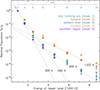 |
Fig. 7. Population levels for several apertures. The level populations derived from the extracted fluxes show that these fall into two groups. The dashed lines for single temperatures of 300 K, 400 K, 900 K and 1200 K characterise the temperature range probed by the lines. |
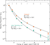 |
Fig. 8. Fits for a power-law temperature distribution. Fits to the star forming arc in the circumnuclear ring and the hotspot in the ionisation cone, show they can be well characterised by such a distribution. |
5.1. Thermal equilibrium models
We have extracted fluxes of the S(1) to S(8) lines in the apertures indicated in Fig. 5. The derived population levels N/g are shown in Fig. 7 as a function of the energy of the level (as a temperature). These fall into two distinct groupings, neither of which can be characterised by a single temperature. The populations for the star forming arc, eastern knot, and southern region have similar distributions, and indicate the gas is relatively warm, with temperatures in the range 300–900 K. The nucleus and hotspot are warmer still, in the range 400–1200 K.
Although the data can be characterised by two temperatures, a more physical approach is to adopt a power-law temperature distribution dN = T−βdT, where N is the gas column density (Zakamska 2010; Pereira-Santaella et al. 2014; Togi & Smith 2016). Applying this method yields the fits in Fig. 8. In all cases the J = 5 level is below the fit, but that is because the corresponding S(3) line at 9.66 μm is affected by the silicate absorption. The result here is that the star forming arc, eastern knot, and southern region have power-law indices in the range β = 5.5–6.0, while the nucleus and hotspot have significantly shallower indices of β = 4.4–4.5 indicating a larger fraction of warmer gas. Considering the contributions of gas at different temperatures to each level, as illustrated in Fig. 7, these models indicate that the S(1) line flux is dominated by gas at temperatures of 200 K or slightly less while S(7) is dominated by gas at 1400–1600 K. Since the lines we observe are insensitive to gas at temperatures below ∼200 K, care needs to be taken if extrapolating the power-law index to lower temperatures. Indeed, by simultaneously fitting CO and H2 line distributions, Pereira-Santaella et al. (2014) have shown that, at least in Seyfert LIRGs, a flatter index is appropriate at T < 200 K.
The initial studies adopting a power-law index to characterise the rotational H2 lines focused on ultra-luminous infrared galaxies (ULIRGs). Zakamska (2010) found indices in the range β = 2.5–5.0 could reproduce the variety of observed excitation diagrams, while Pereira-Santaella et al. (2014) derived values consistent with only the top end of that range. The sample of Togi & Smith (2016) was largely based on the Spitzer Infrared nearby Galaxies Survey (Kennicutt et al. 2003) and so contained a wider variety of objects (LINERs and Seyferts, as well as HII and dwarf galaxies) to which some radio galaxies and a quasar were added. They found values for β in the range 4–6, with an average of β = 4.8 ± 0.6 for the SINGS galaxies. More recently, in the circumnuclear region of NGC 7469, Zhang & Ho (2023) found values varying from 5 at a radius of 600 pc to 4 at the nucleus. The range of β values we find in all five apertures are consistent with these and may be associated with a shock origin for the heating mechanism. This was explicitly addressed by Pereira-Santaella et al. (2014), who applied the same analysis to models of line emission calculated for gas that cools radiatively after it has been heated at a constant rate to a temperature that is dependent on the adopted shock velocity. For gas densities nH2 ≳ 105 cm−3 they found β ≳ 4. In contrast, they found that PDR models yielded rather high values of β > 10. Nevertheless, they argued that PDR emission may be needed to account for the CO emission line ratios, and that a combination of the two processes was likely. We will return to the topic of shock excitation, and take a more detailed look at it, in Sect. 5.4.
5.2. Excitation distribution: jet or disk interaction?
Looking at the spatially resolved H2 excitation distribution can help to assess whether it is heated by an interaction of the disk with the jet or the ionisation cone. The integral field capability of the MRS enables us to do so in a simple but robust way, deriving the excitation from the ratio of a pair of H2 lines. Because the S(3) line is close to 10 μm and hence affected, particularly in the very centre, by silicate absorption (see Sect. 5.3), we have used the ratio of the S(1) and S(5) lines. The analysis above shows that this can be considered as a characteristic temperature, or equivalently as indicative of the index for a power-law distribution at each location. Adopting the former representation, the temperature map we derive is shown in Fig. 9.
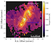 |
Fig. 9. H2 excitation map. Map of molecular gas temperature derived from the S(1)/S(5) line ratio (shown at the 0.20″ pixel scale of the S(1) line). This characteristic temperature also represents the distribution of temperatures at each location. The comparison to the [Fe II] and [Fe VII] lines (white and blue contours respectively) show that the warmer H2 emission traces the edge rather than bulk of the ionisation cone. Specifically, it traces the northern edge of the western cone and the southern edge of the eastern cone. |
It is difficult to make conclusive statements about whether this is the result of an interaction between the jet and disk. In favour of such an explanation is the brightening of the jet at a distance of about 2.5″ from the core (Fig. 4), which is close to the hotspot at a radius of 1.8″ (region 2 in Fig. 5), suggesting a possible link between these phenomena. However, it is difficult to associate the jet with the remarkable coincidence between the location of the warmest H2 and the edge of the ionisation cone that is revealed by Fig. 9. Here, the high excitation [Fe VII] 9.53 μm line (blue contours) traces the bulk of the ionisation cone, while the low excitation [FeII] 5.34 μm line (white contours) traces an X-shape corresponding to the partially ionised zone at its edges. The excitation map very clearly follows the edge of the ionisation cone, but only on one side: to the west it matches the northern edge but is absent on the southern edge, while to the east it matches the southern edge but is absent on the northern edge. As discussed by Shimizu et al. (2019), the disk of NGC 5728 rotates in a clockwise direction. And hence, on the western side of the disk, gas enters the ionisation cone from the north. Similarly, on the eastern side of the disk, gas rotates into the ionisation cone from the south. The H2 temperature map is tracing these specific boundaries. The spatial coincidence with the [FeII] emission along these edges suggests that the molecular gas in the disk is heated as it enters the ionisation cone, as the clouds in the disk collide with gas that is being accelerated outwards by the AGN.
Both of the processes discussed above could be a source of shocks, which would be consistent with the expectation from Sect. 5.1. And while we can only use qualitative arguments, it seems plausible that both are involved: the jet-disk interaction creating the hotspot to the north-west of the AGN, and the rotation of disk gas into the ionisation cone to explain the asymmetric one-sided heating.
Additional line fluxes measured in the nuclear aperture.
Parameters from LTE models of the H2 line ratios.
5.3. Non-LTE model of the nuclear region
We can extend the analysis of the nucleus itself by including seven ro-vibrational v = 14-0 and v = 2–1 observed in the K-band with SINFONI, given in Table 2. These were measured from the reduced cubes analysed by Shimizu et al. (2019), who only included the 1-0 S(1) line in their work. Estimating the extinction to the line emitting region is important here because of its differential effect between the near-infrared and mid-infrared lines. We therefore include the Brγ line from SINFONI and the Pfα line from the MRS spectrum. We have considered three prescriptions for the extinction curve: Rosenthal et al. (2000) towards the Orion Molecular Cloud, Chiar & Tielens (2006) for the local ISM, and Fritz et al. (2011) towards the Galactic Center. The overall shapes of these curves across the 2–20 μm range are similar, the major difference being their treatment at 8–12 μm where silicate absorption is prominent, and which in our analysis only affects the S(3) line. Trying these different curves yields consistent fits to the extinction corrected data, well within the uncertainties from the measurements themselves, and so for the discussion here we simply adopt that of Fritz et al. (2011). From the ratio of the Brγ and Pfα lines we find ABrγ = 0.78 mag. The impact is relatively modest in the infrared, although it would imply the nucleus is not visible at optical wavelengths. The main effect is in the silicate absorption band, modifying the ratio of S(3)/S(1) by a factor 2.6, and the differential reddening, which is a factor 1.4 between the near- and mid-infrared from 1-0 S(1) to 0-0 S(1).
The full set of H2 transitions cannot be fit with an LTE model that has a single power-law temperature distribution. We therefore drop the assumption of LTE. Doing so is physically motivated because the ro-vibrational lines have much higher critical densities and hence are not necessarily thermalised. Indeed, observations of AGN show evidence of non-thermal line ratios in the v = 2–1 transitions (Davies et al. 2005). As such, the volume density of H2 becomes a parameter of the model. In addition, because the critical densities for these transitions are lower by 2-3 orders of magnitude when considering H as the perturber rather than H2 (Le Bourlot et al. 1999), the density of the neutral component must also be included. The model we adopt here is described in Pereira-Santaella et al. (2014) which makes use of RADEX (van der Tak et al. 2007). The grids considered cover kinetic temperatures Tkin = 10–2800 K, H2 density nH2 = 102–109 cm−3, ratio nH/nH2 = 1–10−5. The ortho-to-para ratio adopted varies between 0 for low temperatures and 3 for Tkin > 200 K (see Burton et al. 1992). These models are then used with a power-law temperature distribution as described above.
Fig. 10 shows that the full set of transitions can be fit with a single power law temperature distribution. In this case we find β = 3.6, slightly flatter than, but consistent with, the result for the LTE fit to the rotational transitions. The densities yielded by the fit, of nH2 = 104.5 cm−2 and nH = 103.4 cm−2, are needed to match the relative populations between the vibrational levels in the absence of any external influence. However, the figure also shows that the v = 1–0 transitions are thermalised, while there are indications for non-thermal processes in the v = 2–1 transitions: the J = 4 level is high with respect to J = 3 and J = 5 as expected for an ortho-para-ratio < 3. This model would need an additional component – such as an external UV field – to achieve that. Similar effects have been reported before for AGN, where they were interpreted as due to a dense PDR (Davies et al. 2005). Here, the power-law index and densities are consistent with the calculation performed by Pereira-Santaella et al. (2014) for shocked gas. We therefore explore whether shocks, perhaps illuminated by an external UV field, may be the origin of the line emission.
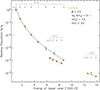 |
Fig. 10. Non-LTE fit with a power-law temperature distribution. The model was fitted to the nuclear H2 populations derived from the rotational and vibrational lines, after correcting for extinction. In this case, the volume density of both H2 and H are derived because of their influence on collisional de-excitation. |
5.4. Shock models of the nuclear region
In order to assess whether shock models are consistent with the observed line emission, we use the library of models calculated by Kristensen et al. (2023), which are based on models of Flower et al. (1985) and Godard et al. (2019). These authors note that the rotational H2 lines alone are unlikely to strongly constrain the grid of models, and so we have limited this analysis to the nuclear region (Fig. 5) where we can combine the v = 0–0, v = 1–0 and v = 2–1 transitions. In addition, rather than focus solely on the model with minimum χ2, we consider the properties of all of the models with lower χ2. Among the matches with the lowest χ2 are two groups of models, an example of each of which is shown in Fig. 11. Each of these groups points to a characteristic density nH, shock speed Vs, magnetic field strength b and radiation intensity G0, while the cosmic ionisation rate ζ and PAH abundance are unconstrained.
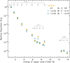 |
Fig. 11. Potential shock models. Two families of shock models from Kristensen et al. (2023) are a reasonable match to the nuclear H2 populations (after correcting for extinction). Their main parameters (density nH, velocity Vs, magnetic field scaling factor b, and radiation field G0) are indicated. |
One model group, denoted by green plus signs, represents a higher velocity Vs = 60 km s−1 shock in a lower density log nH (cm−3) = 2 medium (note that Vs represents the shock speed internal to the clouds and is not necessarily indicative of the bulk cloud speed). This remains a C-shock because the magnetic field scaling factor b = 3 is relatively high (the magnetic field B in the models is transverse, given by  , here corresponding to 30 μG). Only a weak interstellar radiation field G0 = 0.1 is required because the density is too low to thermalize the 2-1 levels. This model matches the ro-vibrational levels very well, and also the lower rotational levels. However, it fails for the J = 9 and J = 10 levels, under-predicting these levels by a factor 2–4. This indicates that the temperature distribution of the gas is too steep; and if one were able to measure the populations of higher rotational levels these would probably be even more significantly under-estimated by the model. For this reason we consider this model less likely.
The other model group, denoted by blue crosses, represents lower velocity Vs = 30 km s−1 shock in a higher density log nH (cm−3) = 5 medium. This higher density matches the expectation from our previous analysis much better. While the magnetic field scaling parameter b = 1 is lower, the higher density means the actual magnetic field is also higher at B = 300 μG. Finally, this group of models has a very significant incident radiation field G0 = 103, which is the cause of the non-thermal signature of the v = 2–1 levels. So close to the AGN, the origin of the high radiation field is expected to be the AGN itself. For this model, the typical difference to the data is a factor 1.3, with a maximum of only 1.7, and so we consider it more representative of the full data set. That the fit is not better is a combination of the coarse spacing in the model grid and that within the aperture of area of ∼0.1 kpc2 it is likely more than one excitation process is at work.
While these models appear to support the contention that the disk gas has been shock heated (e.g. by the jet or as it rotates into the ionisation cone), we need to assess whether the H2 line luminosities are consistent with that of CO (2-1) or whether there is additional cold molecular gas that is not shock heated. This can be done by a comparison of their respective column densities.
5.5. Gas column density
The LTE fits discussed in Sect. 5.1 indicate column densities (2H2 + H) in the range log NH (cm−2) = 20.5–21.5, where the highest value is for the nuclear aperture. The column inferred from the more detailed non-LTE analysis of the nucleus in Sect. 5.3 is consistent with this at log NH = 21.4. However, a caveat for these estimates is that the models were truncated at a lowest temperature of 200 K, meaning that any substantial gas component at a significantly cooler temperature is not included. This is important to bear in mind when comparing the column densities to those implied by the shock models discussed in Sect. 5.4. Our preferred model yields log NH = 21.3, although the relative contribution of H and H2 to this total is rather different. We assign this to the impact of the external UV field in the shock model, which helps to adjust the relative vibrational levels without needing to rely solely on collisional processes. Since the shock model integrates the full gas column, this similarity means that within the nuclear aperture the bulk of the gas in the model must be at ≳200 K – a situation that should be expected since the post-shock temperature is > 200 K. We can confirm this by considering the J < 3 populations in the shock model. These are within 10% of an isothermal line with a temperature of about 370 K, indicating that, despite their lower excitation energies, they do not trace cooler gas components than the J = 3 population.
Given the similarity of the H2 rotational populations between the nucleus and the hotspot, we apply the same shock model to the hotspot and compare the column densities. Based on the fit for a power-law temperature distribution in LTE, we find log NH = 20.6 (Table 3), consistent with the log NH = 20.6 obtained by scaling the shock model to the observed flux. Thus the simple LTE analysis of this extra nuclear region is consistent with the same shock model that matches the more detailed data available for the nucleus.
We now turn to the CO (2-1) emission reported in Shimizu et al. (2019). Those authors adopted a CO-to-H2 ratio of αCO = 1.1 typical for the central regions of nearby galaxies. However, in a detailed study of NGC 3351, Teng et al. (2022) found that while this is what one might expect when integrating over the whole central region, αCO shows substantial variations from region to region. In particular, they found that in turbulent flows, the average could be an order of magnitude lower. They explained this in terms of the higher velocity dispersion leading to lower optical depths and a larger fraction of the CO emission being able to escape. Although CO (2-1) is not detected in the outflow in a spatially resolved sense, integrating over the hotspot aperture provides a marginal detection that would yield a column density similar to that above if one adopts αCO ∼ 0.3. Low values comparable to this have been reported by other authors, such as Pereira-Santaella et al. (2024) who derived αCO ∼ 0.4 − 0.6 in the molecular outflow of NGC 3256 using the CO v = 1–0 4.67 μm band observed with NIRSpec, and Teng et al. (2022) who found αCO < 0.1 in turbulent inflowing gas in NGC 3351 based on multiple CO, 13CO and C18O transitions. In our case, it would imply that all the molecular gas in the outflow is heated by the shock, and no cold component remains. As such, the CO (2-1) line is weak but one might expect to detect higher transitions. However, in the nuclear aperture, using the same value of αCO yields log NH = 22.3, which is an order of magnitude higher than indicated by the analysis of the H2 rotational lines. This strongly suggests there is an additional cold component in the nucleus. This is apparent in the CO (2-1) map in Fig. 4 as a transverse component, which was identified as Comp2 by Shimizu et al. (2019). They described it as a warped inner rotating molecular disk that contributes to shaping the bicone and provides the material fuelling the AGN, and is associated with the higher extinction at the nucleus. More recent data with beam sizes of 0.2–0.4″ in the CO (1-0), CO (2-1), and CO (3-2) transitions spatially resolve this highly inclined disk, and indicate that the typical physical conditions correspond to nH ∼ 102 − 105 cm−3 and Tkin ∼ 10 − 50 K (García-Burillo et al. in prep.). Thus, in contrast to the hotspot region, in the nuclear aperture, the shock excited H2 rotational lines do not trace the full gas column.
Our conclusion is that the available evidence points to a scenario in which the molecular gas in the ionisation cone is excited both by shocks and UV radiation from the AGN. Because the bulk of the molecular gas in the outflow is shock heated, the CO (2-1) line is no longer a good tracer. In the central arcsec, while the H2 rotational lines still trace the shocked gas, the CO line emission is strong because it is dominated by a separate highly inclined disk.
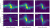 |
Fig. 12. Position-velocity diagrams along the outflow. A pseudo-slit width of 1″at a position angle of −60 deg East of North was used to extract PV diagrams for the H2 0-0 S(1), S(3), S(5), CO (2-1), [Ne II], and [Ne VI] emission lines. In each case the continuum has been subtracted (although a residual from wiggles in the continuum can be seen in the panel for the S(1) line). Overplotted are the best fit rotating disk model from (Shimizu et al. 2019, dashed red line) and the best fit rotating disk with a planar radial outflow described in Sect. 6.1 for the S(5) line (solid red line). At large radii, all lines trace only the pure rotation while the inner regions need an outflow component. The molecular gas kinematics can be modelled well with a planar radial outflow while the ionised gas clearly has a separate high velocity, compact outflow being lifted off the disk. As comparison numbers for the CO line, outside the central 1–2″ the circular velocity is around 300 km s−1 while the dispersion is typically 15 km s−1. |
6. Molecular gas kinematics: a terminated outflow
In this Section we return to Fig. 4, the key points of which were briefly summarised in Sect. 4.3. We begin by comparing the flux and kinematics maps of the rotational H2 lines to those of the CO (2-1) line, and then compare the molecular outflow to the ionised outflow. We show that the outflow terminates because it decelerates completely, and we assess what mechanisms may be responsible for that.
6.1. Planar molecular flow
Nearly all the features and detailed structure visible in the S(1) map (top left panel of Fig. 4) are matched in the CO (2-1) map (bottom left panel). The only differences are the detection of molecular gas in the ionisation cones where the CO surface brightness is below the detection limit and, perhaps related to this, enhanced S(1) emission in a location we have identified as the ‘eastern knot’ (region 3 in Fig. 5). Together with the similarities of their velocity maps, as well as of the detailed structure in their dispersion maps, this indicates that the S(1) and CO lines are largely tracing the same component of molecular gas.
The higher rotational lines are qualitatively different, as one might expect from the excitation analysis in Sect. 5. Most notably, the flux distributions of the S(3) and S(5) lines shown are more prominent in the direction of the ionisation cone and outflow, with the additional hotspot feature (region 2 in Fig. 5) becoming apparent to the north-west.
The velocity fields of all the H2 lines are similar to that of the CO line, showing apparent rotation but with a twist in the zero-velocity contour. A simple disk model, tracing the rotational velocity component, was fitted to the CO map on large scales by Shimizu et al. (2019). The right-hand column of Fig. 4 shows the velocity fields after subtracting this disk model, and clearly reveals a residual in the direction of the ionisation cone indicative of outflowing gas. We explore this phenomenon in Fig. 12. Each panel contains a position-velocity (PV) plot extracted along the direction of the outflow. Overplotted as a dashed red line is the line-of-sight velocity of the rotation in the disk model. At the edges of the extracted region, at ±4″ corresponding to the radius of the star forming circumnuclear ring, the observed velocities match the model. But at smaller radii there is a clear discrepancy in the H2 and CO lines, with a projected velocity of up to ∼200 km s−1, tracing the molecular outflow. This can be matched very well if one adds a planar radial component vrad to the disk model (noting that this is the bulk velocity of the clouds, and is different to the shock velocity within the clouds discussed previously). The solid red line in the panels shows the resulting line-of-sight velocity for
where the radial velocity vrad reaches its maximum vmax = 400 km s−1 at r0 = 50 pc, before decreasing back to vrad = 0 at rout = 750 pc. The differing central slopes are due to the different beam smearing impacts of the PSF over the wide wavelength range of the lines shown. That this simple prescription matches the observed PV plots reasonably well suggests that there is a finite extended acceleration zone out to about 50 pc, and beyond that the gas gradually decelerates over a distance of ∼700 pc. Because, the outflow is oriented so close to the disk plane (see Sect. 2), and because the velocity trajectory re-joins that of the disk rotation, we conclude that the molecular outflow is in the plane of the disk.
This outflow is both modest in velocity and limited in spatial extent, terminating within 1 kpc. It is very different from the ionised outflow that has been discussed extensively in the literature. The steep trajectory on the PV diagram can be seen clearly for the [Ne VI] line, reaching a projected velocity of > 700 km s−1 (compared with 200 km s−1 for the molecular gas) within 1″. And the line emission fades without indicating any tendency to revert back to the disk rotation velocity, suggesting that the ionised gas is escaping the local (few hundred parsec scale) environment. It is instead more similar in both velocity and extent to the molecular outflows reported in other galaxies. Davies et al. (2014) reported molecular outflow velocities in the range 130–190 km s−1 for several galaxies, but these were based on ro-vibrational H2 lines tracing the hottest component of the molecular gas. Ramos Almeida et al. (2022) analysed the CO (2-1) line in seven nearby QSOs, find co-planar outflows with slightly higher velocities in the range 200–350 km s−1 extending out to 400–1300 pc. Detailed modelling of CO (3-2) and CO (2-1) in several other galaxies continues the emerging trend of planar molecular outflows at velocities up to ∼200 km s−1 on scales of several hundred parsecs. Specifically, for NGC 3227, Alonso-Herrero et al. (2019) report evidence for a planar outflow at 180 km s−1 out to 70 pc; for NGC 7171, Alonso-Herrero et al. (2023) find radial outflow velocities as high as 80–100 km s−1, decreasing out towards 900 pc; and for NGC 5506, Esposito (2024) find more modest radial velocity of 50 km s−1 at 50 pc, decreasing to 25 km s−1 and extending out to 600 pc. The spatial extents of these outflows and that reported here are comparable, as is the indication that the outflow velocity decreases towards larger radii. That the peak value we find of 400 km s−1 is higher than for some of these other galaxies may be due to two reasons. The simple two component model we use leads to a high peak at small radii that is reduced by beam smearing (and projection effects) in the data, and a more physical model may have a flatter profile. In addition, we have modelled the outflow specifically in one direction, while in some cases an azimuthally symmetric outflow has been adopted. It is currently not clear whether this difference reflects a true disparity in the driving mechanism of the outflow or will be reconciled with additional high resolution data, but it seems likely that it should have an impact on the inferred velocities and outflow rates.
6.2. Gas acceleration and deceleration
In this section we look at what might cause the deceleration of the molecular gas. We focus on two inevitable mechanisms, the increasing gravitational potential and mass-loading due to swept up ambient gas; and consider what happens to a parcel of gas that is accelerated radially and then decelerated while it remains in the outflow region. The deceleration mechanisms are inter-dependent and so cannot be considered separately.
We can infer the impact of the gravitational potential by deriving the mass profile of the galaxy from the rotation curve of the disk model fitted to the CO velocity field (Shimizu et al. 2019). Throughout most of the disk, gas is supported by rotation. But in the outflow, if the gas moves outward, this is no longer the case, and we can calculate the corresponding deceleration term. At the same time the gas parcel will sweep up ambient gas, which will also cause a deceleration if we assume the collisions are inelastic and that momentum is conserved. However, the ambient gas has a tangential velocity matching the disk rotation at each radius. And, again due to momentum conservation, this will tend to increase the tangential velocity of the gas parcel, hence providing greater support against the increased gravitational potential. It is these interactions that may cause at least some of the shock heating discussed in Sect. 5.
In addition to mechanisms that decelerate the gas parcel, there must be an acceleration term causing it to move outwards at all. We adopt a simple prescription that the acceleration is constant out to 25 pc, and then decreases inversely proportionally to the radius. This is not based on any physical principle, but is intended only as a conceptual representation that can match the observed velocity profile. As noted in Sect. 2, the source of the gas that is being accelerated is within the inner 200 pc scale disk. This means that the outflow is constantly replenished as gas from that inner structure is re-injected back onto circumnuclear scales. This process can continue until the gas reservoir is exhausted and the AGN turns off.
A combination of all three terms is given by the solid blue line in Fig. 13. These can provide the rapid acceleration to about 400 km s−1 followed by a roughly linear decline over the subsequent 600 pc. In this toy model, the gas parcel begins with zero radial and tangential velocity. It is initially accelerated directly outwards, but after about 2 Myr the interaction with the rotating ambient gas means its mass has increased by a factor ∼2, transferring angular momentum so that it is increasingly moving tangentially. This timescale is similar to what one would expect for the crossing time of the ionisation cone, given the rotation velocity at this radius of ∼300 km s−1 and the ∼600 pc width of the region. After this time, the gas parcel moves mostly in the tangential direction. The toy model does not explore what happens once the gas leaves the ionisation cone, but indicates that further mass-loading can increase its tangential velocity until it becomes much more similar to the rotation velocity of the ambient disk.
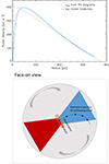 |
Fig. 13. Toy model of the outflow deceleration. Top panel: radial velocity of the H2 as a function of distance from the centre along the ionisation cone. The dashed grey line represents the simple description given in Eq. (1) and Fig. 12. The solid blue line is a toy model described in Sect. 6.2, illustrating that this trajectory can be qualitatively assigned to a combination of the increasing gravitational potential and mass-loading. Bottom panel: characteristic spatial trajectory of a cloud described by the toy model, where the black circles indicate 0.5 Myr intervals. Initially the motion is radially outwards, but as the cloud decelerates the momentum imparted by mass-loading diverts it to tangential motion. |
It is not possible to propose a unique solution here, since gas is accelerated over a range of angles and even the highly simplified picture above still has many parameters, without enough constraints. Instead, our aim is to argue that the observed radial velocity profile can be reproduced by a combination of continuous acceleration in a way that decreases with radius beyond a break point, and which is counteracted by deceleration due to both the increasing gravitational potential and mass-loading by swept up ambient gas; and that all of these effects are required.
7. Conclusions
As part of a larger study of nearby AGN, we present an analysis of the spatially resolved excitation and kinematics of the rotational H2 lines in the central kiloparsec of the Seyfert 2 galaxy NGC 5728, observed with JWST/MIRI MRS at 5–28 μm. Our main findings are that:
-
H2 is directly detected throughout the ionisation cone, where previous observations had not detected the millimetre CO (2-1) line. The gas in the ionisation cone is warmer than in the surrounding regions, or equivalently has a flatter power law index tracing its temperature distribution.
-
Shocks appear to be heating the molecular gas as indicated by the good match between shock models and the H2 level populations, including 0-0, 1-0 and 2-1 vibrational levels. The shock models include UV excitation, which is expected from the AGN. The spatially resolved excitation map supports this, showing that the warmest gas is concentrated (i) along the edges of the ionisation cone into which ambient disk gas is rotating, and (ii) in a region close to where the jet brightens, suggestive of a jet-disk interaction.
-
The molecular gas shows a clear signature of radial flow, which is very different from the outflow traced by the ionised emission lines. It is accelerated over a short distance but then decelerates, suggesting the molecular gas remains in the disk plane. The deceleration mechanisms of this outflow include the effects of the gravitational potential and mass-loading as ambient gas is swept up.
-
A spectro-astrometric signature is measured, indicative of a spatially resolved absorbing structure on scales of ∼20 pc. This is slightly misaligned with respect to the 200 pc scale edge-on disk that delineates the direction of the outflow, and may be the reason for asymmetric illumination of the circumnuclear disk at one edge of the ionisation cone.
The term ‘ionisation potential’ can be ambiguous when applied to emission lines. In some cases an emission line arises following recombination from the next higher ionisation level. Here we are considering fine structure lines, which originate from collisional excitation with electrons, and so the ionisation potential refers to the ion’s current state.
Acknowledgments
MTL, CP, EKSH, and LZ acknowledge grant support from the Space Telescope Science Institute (ID: JWST-GO-01670.007-A). AAH, LHM, and MVM research has been funded by grant Nr. PID2021-124665NB-I00 by the Spanish Ministry of Science and Innovation/State Agency of Research MCIN/AEI/ 10.13039/501100011033 and by “ERDF A way of making Europe”. BG-L acknowledges support from the Spanish State Research Agency (AEI-MCINN/10.13039/501100011033) through grants PID2019-107010GB-100 and PID2022-140483NB-C21 PID2022-138560NB-I00, and the Severo Ochoa Program 2020-2023 (CEX2019-000920-S). CR acknowledges support from Fondecyt Regular grant 1230345 and ANID BASAL project FB210003. CRA thanks support by the EU H2020-MSCA-ITN-2019 Project 860744 “BiD4BESt: Big Data applications for black hole Evolution STudies” and by project PID2022-141105NB-I00 “Tracking active galactic nuclei feedback from parsec to kiloparsec scales”, funded by MICINN-AEI/10.13039/501100011033. DR acknowledges support from STFC through grants ST/S000488/1 and ST/W000903/1. EB acknowledges the María Zambrano program of the Spanish Ministerio de Universidades funded by the Next Generation European Union and is also partly supported by grant RTI2018-096188-B-I00 funded by the Spanish Ministry of Science and Innovation/State Agency of Research MCIN/AEI/10.13039/501100011033. MPS acknowledges support from grant RYC2021-033094-I funded by MCIN/AEI/10.13039/501100011033 and the European Union NextGenerationEU/PRTR. MS acknowledges support by the Ministry of Science, Technological Development and Innovation of the Republic of Serbia (MSTDIRS) through contract no. 451-03-66/2024-03/200002 with the Astronomical Observatory (Belgrade). RD thanks M. Durré for help with the radio maps and VLA archive. The 6 cm NVAS image of NGC 5728 was produced as part of the NRAO VLA Archive Survey, which can currently be browsed through http://www.vla.nrao.edu/astro/nvas. This work is based on observations made with the NASA/ESA/CSA James Webb Space Telescope. The data were obtained from the Mikulski Archive for Space Telescopes at the Space Telescope Science Institute, which is operated by the Association of Universities for Research in Astronomy, Inc., under NASA contract NAS 5-03127 for JWST; and from the European JWST archive (eJWST) operated by the ESAC Science Data Centre (ESDC) of the European Space Agency. These observations are associated with program #1670.
References
- Alonso-Herrero, A., Pereira-Santaella, M., García-Burillo, S., et al. 2018, ApJ, 859, 144 [Google Scholar]
- Alonso-Herrero, A., García-Burillo, S., Pereira-Santaella, M., et al. 2019, A&A, 628, A65 [NASA ADS] [CrossRef] [EDP Sciences] [Google Scholar]
- Alonso-Herrero, A., García-Burillo, S., Hönig, S. F., et al. 2021, A&A, 652, A99 [NASA ADS] [CrossRef] [EDP Sciences] [Google Scholar]
- Alonso-Herrero, A., García-Burillo, S., Pereira-Santaella, M., et al. 2023, A&A, 675, A88 [NASA ADS] [CrossRef] [EDP Sciences] [Google Scholar]
- Argyriou, I., Glasse, A., Law, D. R., et al. 2023, A&A, 675, A111 [NASA ADS] [CrossRef] [EDP Sciences] [Google Scholar]
- Asmus, D., Hönig, S. F., Gandhi, P., Smette, A., & Duschl, W. J. 2014, MNRAS, 439, 1648 [NASA ADS] [CrossRef] [Google Scholar]
- Audibert, A., Ramos Almeida, C., García-Burillo, S., et al. 2023, A&A, 671, L12 [NASA ADS] [CrossRef] [EDP Sciences] [Google Scholar]
- Baumgartner, W. H., Tueller, J., Markwardt, C. B., et al. 2013, ApJS, 207, 19 [Google Scholar]
- Burton, M. G., Hollenbach, D. J., & Tielens, A. G. G. 1992, ApJ, 399, 563 [NASA ADS] [CrossRef] [Google Scholar]
- Caglar, T., Burtscher, L., Brandl, B., et al. 2020, A&A, 634, A114 [NASA ADS] [CrossRef] [EDP Sciences] [Google Scholar]
- Canzian, B. 1993, ApJ, 414, 487 [NASA ADS] [CrossRef] [Google Scholar]
- Chiar, J. E., & Tielens, A. G. G. M. 2006, ApJ, 637, 774 [NASA ADS] [CrossRef] [Google Scholar]
- Cicone, C., Maiolino, R., Sturm, E., et al. 2014, A&A, 562, A21 [NASA ADS] [CrossRef] [EDP Sciences] [Google Scholar]
- Davies, R. I., Sternberg, A., Lehnert, M. D., & Tacconi-Garman, L. E. 2005, ApJ, 633, 105 [CrossRef] [Google Scholar]
- Davies, R. I., Maciejewski, W., Hicks, E. K. S., et al. 2009, ApJ, 702, 114 [NASA ADS] [CrossRef] [Google Scholar]
- Davies, R., Mark, D., & Sternberg, A. 2012, A&A, 537, A133 [NASA ADS] [CrossRef] [EDP Sciences] [Google Scholar]
- Davies, R. I., Maciejewski, W., Hicks, E. K. S., et al. 2014, ApJ, 792, 101 [Google Scholar]
- Davies, R. I., Burtscher, L., Rosario, D., et al. 2015, ApJ, 806, 127 [Google Scholar]
- Davies, R., Baron, D., Shimizu, T., et al. 2020, MNRAS, 498, 4150 [Google Scholar]
- Díaz-Santos, T., Charmandaris, V., Armus, L., et al. 2011, ApJ, 741, 32 [Google Scholar]
- Donnan, F. R., García-Bernete, I., Rigopoulou, D., et al. 2024, ArXiv e-prints [arXiv:2402.17479] [Google Scholar]
- Durré, M., & Mould, J. 2018, ApJ, 867, 149 [Google Scholar]
- Durré, M., & Mould, J. 2019, ApJ, 870, 37 [Google Scholar]
- Ellison, S. L., Wong, T., Sánchez, S. F., et al. 2021, MNRAS, 505, L46 [NASA ADS] [CrossRef] [Google Scholar]
- Esposito, F. 2024, A&A, accepted [Google Scholar]
- Fabian, A. C. 2012, ARA&A, 50, 455 [Google Scholar]
- Feruglio, C., Fabbiano, G., Bischetti, M., et al. 2020, ApJ, 890, 29 [Google Scholar]
- Fiore, F., Feruglio, C., Shankar, F., et al. 2017, A&A, 601, A143 [NASA ADS] [CrossRef] [EDP Sciences] [Google Scholar]
- Flower, D. R., Pineau des Forets, G., & Hartquist, T. W. 1985, MNRAS, 216, 775 [NASA ADS] [CrossRef] [Google Scholar]
- Fluetsch, A., Maiolino, R., Carniani, S., et al. 2019, MNRAS, 483, 4586 [NASA ADS] [Google Scholar]
- Fluetsch, A., Maiolino, R., Carniani, S., et al. 2021, MNRAS, 505, 5753 [NASA ADS] [CrossRef] [Google Scholar]
- Fritz, T. K., Gillessen, S., Dodds-Eden, K., et al. 2011, ApJ, 737, 73 [Google Scholar]
- Gallimore, J. F., Elitzur, M., Maiolino, R., et al. 2016, ApJ, 829, L7 [Google Scholar]
- García-Bernete, I., Rigopoulou, D., Alonso-Herrero, A., et al. 2022, A&A, 666, L5 [NASA ADS] [CrossRef] [EDP Sciences] [Google Scholar]
- García-Bernete, I., Alonso-Herrero, A., Rigopoulou, D., et al. 2024, A&A, 681, L7 [NASA ADS] [CrossRef] [EDP Sciences] [Google Scholar]
- García-Burillo, S., Combes, F., Usero, A., et al. 2014, A&A, 567, A125 [Google Scholar]
- García-Burillo, S., Alonso-Herrero, A., Ramos Almeida, C., et al. 2021, A&A, 652, A98 [NASA ADS] [CrossRef] [Google Scholar]
- Gardner, J. P., Mather, J. C., Abbott, R., & Zondag, E. 2023, PASP, 135, 068001 [CrossRef] [Google Scholar]
- Godard, B., Pineau des Forêts, G., Lesaffre, P., et al. 2019, A&A, 622, A100 [NASA ADS] [CrossRef] [EDP Sciences] [Google Scholar]
- Imanishi, M., Nguyen, D. D., Wada, K., et al. 2020, ApJ, 902, 99 [CrossRef] [Google Scholar]
- Impellizzeri, C. M. V., Gallimore, J. F., Baum, S. A., et al. 2019, ApJ, 884, L28 [NASA ADS] [CrossRef] [Google Scholar]
- Kennicutt, R. C. Jr., Armus, L., Bendo, G., et al. 2003, PASP, 115, 928 [NASA ADS] [CrossRef] [Google Scholar]
- Kristensen, L. E., Godard, B., Guillard, P., Gusdorf, A., & Pineau des Forêts, G. 2023, A&A, 675, A86 [NASA ADS] [CrossRef] [EDP Sciences] [Google Scholar]
- Kuo, C. Y., Braatz, J. A., Impellizzeri, C. M. V., et al. 2020, MNRAS, 498, 1609 [NASA ADS] [CrossRef] [Google Scholar]
- Lammers, C., Iyer, K. G., Ibarra-Medel, H., et al. 2023, ApJ, 953, 26 [NASA ADS] [CrossRef] [Google Scholar]
- Lamperti, I., Pereira-Santaella, M., Perna, M., et al. 2022, A&A, 668, A45 [NASA ADS] [CrossRef] [EDP Sciences] [Google Scholar]
- Le Bourlot, J., Pineau des Forêts, G., & Flower, D. R. 1999, MNRAS, 305, 802 [NASA ADS] [CrossRef] [Google Scholar]
- Lutz, D., Sturm, E., Janssen, A., et al. 2020, A&A, 633, A134 [NASA ADS] [CrossRef] [EDP Sciences] [Google Scholar]
- Maciejewski, W. 2004a, MNRAS, 354, 883 [NASA ADS] [CrossRef] [Google Scholar]
- Maciejewski, W. 2004b, MNRAS, 354, 892 [NASA ADS] [CrossRef] [Google Scholar]
- Meenakshi, M., Mukherjee, D., Wagner, A. Y., et al. 2022, MNRAS, 516, 766 [NASA ADS] [CrossRef] [Google Scholar]
- Molina, J., Shangguan, J., Wang, R., et al. 2023, ApJ, 950, 60 [NASA ADS] [CrossRef] [Google Scholar]
- Morganti, R. 2017, Front. Astron. Space Sci., 4, 42 [CrossRef] [Google Scholar]
- Morganti, R., Oosterloo, T., Oonk, J. B. R., Frieswijk, W., & Tadhunter, C. 2015, A&A, 580, A1 [NASA ADS] [CrossRef] [EDP Sciences] [Google Scholar]
- Mukherjee, D., Bicknell, G. V., Wagner, A. Y., Sutherland, R. S., & Silk, J. 2018, MNRAS, 479, 5544 [NASA ADS] [CrossRef] [Google Scholar]
- Oosterloo, T., Raymond Oonk, J. B., Morganti, R., et al. 2017, A&A, 608, A38 [NASA ADS] [CrossRef] [EDP Sciences] [Google Scholar]
- Peralta de Arriba, L., Alonso-Herrero, A., García-Burillo, S., et al. 2023, A&A, 675, A58 [NASA ADS] [CrossRef] [EDP Sciences] [Google Scholar]
- Pereira-Santaella, M., Spinoglio, L., van der Werf, P. P., & Piqueras López, J. 2014, A&A, 566, A49 [NASA ADS] [CrossRef] [EDP Sciences] [Google Scholar]
- Pereira-Santaella, M., Álvarez-Márquez, J., García-Bernete, I., et al. 2022, A&A, 665, L11 [NASA ADS] [CrossRef] [EDP Sciences] [Google Scholar]
- Pereira-Santaella, M., González-Alfonso, E., García-Bernete, I., García-Burillo, S., & Rigopoulou, D. 2024, A&A, 681, A117 [NASA ADS] [CrossRef] [EDP Sciences] [Google Scholar]
- Petitpas, G. R., & Wilson, C. D. 2002, ApJ, 575, 814 [CrossRef] [Google Scholar]
- Ramos Almeida, C., Bischetti, M., García-Burillo, S., et al. 2022, A&A, 658, A155 [NASA ADS] [CrossRef] [EDP Sciences] [Google Scholar]
- Ricci, C., Trakhtenbrot, B., Koss, M. J., et al. 2017, ApJS, 233, 17 [Google Scholar]
- Rieke, G. H., Wright, G. S., Böker, T., et al. 2015, PASP, 127, 584 [NASA ADS] [CrossRef] [Google Scholar]
- Rosario, D. J., Burtscher, L., Davies, R. I., et al. 2018, MNRAS, 473, 5658 [NASA ADS] [CrossRef] [Google Scholar]
- Rosario, D. J., Togi, A., Burtscher, L., et al. 2019, ApJ, 875, L8 [NASA ADS] [CrossRef] [Google Scholar]
- Rosenthal, D., Bertoldi, F., & Drapatz, S. 2000, A&A, 356, 705 [NASA ADS] [Google Scholar]
- Rupke, D. S. N., Gültekin, K., & Veilleux, S. 2017, ApJ, 850, 40 [NASA ADS] [CrossRef] [Google Scholar]
- Schommer, R. A., Caldwell, N., Wilson, A. S., et al. 1988, ApJ, 324, 154 [CrossRef] [Google Scholar]
- Shangguan, J., Ho, L. C., & Xie, Y. 2018, ApJ, 854, 158 [NASA ADS] [CrossRef] [Google Scholar]
- Shangguan, J., Ho, L. C., Bauer, F. E., Wang, R., & Treister, E. 2020, ApJ, 899, 112 [NASA ADS] [CrossRef] [Google Scholar]
- Shimizu, T. T., Davies, R. I., Lutz, D., et al. 2019, MNRAS, 490, 5860 [Google Scholar]
- Shin, J., Woo, J.-H., Chung, A., et al. 2019, ApJ, 881, 147 [Google Scholar]
- Son, D. H., Hyung, S., Ferruit, P., Pécontal, E., & Lee, W. B. 2009, MNRAS, 395, 692 [CrossRef] [Google Scholar]
- Stalevski, M., Asmus, D., & Tristram, K. R. W. 2017, MNRAS, 472, 3854 [NASA ADS] [CrossRef] [Google Scholar]
- Stalevski, M., Tristram, K. R. W., & Asmus, D. 2019, MNRAS, 484, 3334 [NASA ADS] [CrossRef] [Google Scholar]
- Stalevski, M., González-Gaitán, S., Savić, Ð., et al. 2023, MNRAS, 519, 3237 [NASA ADS] [CrossRef] [Google Scholar]
- Sturm, E., González-Alfonso, E., Veilleux, S., et al. 2011, ApJ, 733, L16 [NASA ADS] [CrossRef] [Google Scholar]
- Tadhunter, C. N., Sparks, W., Axon, D. J., et al. 2000, MNRAS, 313, L52 [CrossRef] [Google Scholar]
- Teng, Y.-H., Sandstrom, K. M., Sun, J., et al. 2022, ApJ, 925, 72 [NASA ADS] [CrossRef] [Google Scholar]
- Togi, A., & Smith, J. D. T. 2016, ApJ, 830, 18 [NASA ADS] [CrossRef] [Google Scholar]
- Tombesi, F., Cappi, M., Reeves, J. N., et al. 2010, A&A, 521, A57 [NASA ADS] [CrossRef] [EDP Sciences] [Google Scholar]
- Trindade Falcao, A., Fabbiano, G., Elvis, M., Paggi, A., & Maksym, W. P. 2023, ApJ, 950, 143 [CrossRef] [Google Scholar]
- Tristram, K. R. W., Impellizzeri, C. M. V., Zhang, Z.-Y., et al. 2022, A&A, 664, A142 [NASA ADS] [CrossRef] [EDP Sciences] [Google Scholar]
- van der Tak, F. F. S., Black, J. H., Schöier, F. L., Jansen, D. J., & van Dishoeck, E. F. 2007, A&A, 468, 627 [NASA ADS] [CrossRef] [EDP Sciences] [Google Scholar]
- Veilleux, S., Cecil, G., & Bland-Hawthorn, J. 2005, ARA&A, 43, 769 [NASA ADS] [CrossRef] [Google Scholar]
- Veilleux, S., Meléndez, M., Sturm, E., et al. 2013, ApJ, 776, 27 [Google Scholar]
- Veilleux, S., Maiolino, R., Bolatto, A. D., & Aalto, S. 2020, A&ARv, 28, 2 [NASA ADS] [CrossRef] [Google Scholar]
- Venturi, G., Cresci, G., Marconi, A., et al. 2021, A&A, 648, A17 [NASA ADS] [CrossRef] [EDP Sciences] [Google Scholar]
- Wells, M., Pel, J. W., Glasse, A., et al. 2015, PASP, 127, 646 [NASA ADS] [CrossRef] [Google Scholar]
- Wilson, A. S., Braatz, J. A., Heckman, T. M., Krolik, J. H., & Miley, G. K. 1993, ApJ, 419, L61 [NASA ADS] [CrossRef] [Google Scholar]
- Zakamska, N. L. 2010, Nature, 465, 60 [NASA ADS] [CrossRef] [Google Scholar]
- Zhang, L., & Ho, L. C. 2023, ApJ, 953, L9 [CrossRef] [Google Scholar]
All Tables
All Figures
|
Fig. 1. Circumnuclear region of NGC 5728. Top left: three colour montage of the ALMA CO (2-1) map (red), HST F160WH-band continuum (green), and VLT/MUSE [OIII] line emission (blue). These show several key components: the ionisation cone, and the molecular gas that is collimating it, and the direct illumination of the circumnuclear disk by the AGN. Top centre: B-H dust structure map (from F438W and F160W HST images; there is no strong line contamination in these filters) showing the dusty circumnuclear disk to the west and a lighter region to the east where the outflow has removed dust from our line of sight. Top right: velocity field of the disk model fitted to the ALMA CO (2-1) kinematics. Bottom: cartoon showing two views to illustrate the complex geometry, highlighting that the ionisation cone strongly intersects the galaxy disk (similar to scenario A in Ramos Almeida et al. 2022). All panels are adapted from, or based on the kinematic modelling of, Shimizu et al. (2019). The cartoon has been slightly updated to better match the spatial distributions. |
| In the text | |
|
Fig. 2. Spectro-astrometry of NGC 5728. The relative position of the continuum peaks are shown for right ascension (top) and declination (bottom). The colours demarcate the spectral channels, showing that the datacubes are well aligned spatially and that there is a wavelength dependent shift of the position. For reference, the equivalent measurement for MCG-05-16-023, dominated by a continuum point source and, as is more typical of the sample, showing no spectro-astrometric shifts is also shown as open diamonds (see Esparza-Arredondo et al. in prep.); and the nuclear spectrum is overplotted. |
| In the text | |
|
Fig. 3. Flux and kinematics maps of four neon lines. The flux (left), velocity (centre), and velocity dispersion (right) of the [Ne II] 12.8 μm, [Ne III] 15.6 μm, [Ne V] 24.3 μm, and [Ne VI] 7.7 μm transitions are shown to provide a context about the circumnuclear region of NGC 5728 (north is up, east is left). As the ionisation potential increases from 22 eV to 126 eV (top to bottom), what the line emission traces changes from star formation in the ring to the outflow. The direction of the major kinematic axis and the central dispersion change correspondingly. Interestingly, the outflow kinematics reveal anomalous velocities and unusually high dispersion along the minor axis, which is especially noticeable in the [Ne III] line. |
| In the text | |
|
Fig. 4. Flux and kinematics maps of molecular lines. The flux (far left), velocity (centre left), velocity dispersion (centre right), and residual velocity after subtracting a disk model (far right) are shown for the H2 0-0 S(1), 0-0 S(3), and 0-0 S(5) and 1.3 mm CO (2-1) lines. The CO data and disk model are from Shimizu et al. (2019). In all cases north is up, east is left. These data are the focus of the analysis in Sect. 5 and Sect. 6. The most striking features are: (i) the morphology and kinematics of the CO and S(1) lines are remarkably similar indicating they trace the same gas component, (ii) while CO is not detected in the ionisation cones, the rotational H2 lines are detected with a perturbed velocity field, and (iii) the largest velocity residuals are well-aligned with the ionisation cone as traced by the [Ne V] emission (black contour) and the radio jet at 20 cm (green contours). |
| In the text | |
|
Fig. 5. Apertures used for spectral extractions. These are superimposed on the S(5) flux map (left) and velocity field (right). Rather than being circular, they trace specific features within the overlapping fields of view: (1) the star forming arc, (2) an H2 hotspot in the ionisation cone, (3) a knot of H2 emission to the east, (4) the nucleus, and (5) a region to the south outside the ionisation cone. |
| In the text | |
|
Fig. 6. Mid-infrared spectra in NGC 5728. The spectra for three apertures, corresponding to the nucleus (blue; region 4 in Fig. 5), star forming arc (red; region 1 in Fig. 5), and hotspot (green; region 2 in Fig. 5) are shown on a logarithmic flux scale. The spectra have been extracted from each of the 12 separate datacubes and overplotted. They show that no re-scaling between the cubes is needed. The most prominent lines with reliable identifications have been marked: 36 fine structure lines, 3 H I lines, and 8 H2 lines. |
| In the text | |
|
Fig. 7. Population levels for several apertures. The level populations derived from the extracted fluxes show that these fall into two groups. The dashed lines for single temperatures of 300 K, 400 K, 900 K and 1200 K characterise the temperature range probed by the lines. |
| In the text | |
|
Fig. 8. Fits for a power-law temperature distribution. Fits to the star forming arc in the circumnuclear ring and the hotspot in the ionisation cone, show they can be well characterised by such a distribution. |
| In the text | |
|
Fig. 9. H2 excitation map. Map of molecular gas temperature derived from the S(1)/S(5) line ratio (shown at the 0.20″ pixel scale of the S(1) line). This characteristic temperature also represents the distribution of temperatures at each location. The comparison to the [Fe II] and [Fe VII] lines (white and blue contours respectively) show that the warmer H2 emission traces the edge rather than bulk of the ionisation cone. Specifically, it traces the northern edge of the western cone and the southern edge of the eastern cone. |
| In the text | |
|
Fig. 10. Non-LTE fit with a power-law temperature distribution. The model was fitted to the nuclear H2 populations derived from the rotational and vibrational lines, after correcting for extinction. In this case, the volume density of both H2 and H are derived because of their influence on collisional de-excitation. |
| In the text | |
|
Fig. 11. Potential shock models. Two families of shock models from Kristensen et al. (2023) are a reasonable match to the nuclear H2 populations (after correcting for extinction). Their main parameters (density nH, velocity Vs, magnetic field scaling factor b, and radiation field G0) are indicated. |
| In the text | |
|
Fig. 12. Position-velocity diagrams along the outflow. A pseudo-slit width of 1″at a position angle of −60 deg East of North was used to extract PV diagrams for the H2 0-0 S(1), S(3), S(5), CO (2-1), [Ne II], and [Ne VI] emission lines. In each case the continuum has been subtracted (although a residual from wiggles in the continuum can be seen in the panel for the S(1) line). Overplotted are the best fit rotating disk model from (Shimizu et al. 2019, dashed red line) and the best fit rotating disk with a planar radial outflow described in Sect. 6.1 for the S(5) line (solid red line). At large radii, all lines trace only the pure rotation while the inner regions need an outflow component. The molecular gas kinematics can be modelled well with a planar radial outflow while the ionised gas clearly has a separate high velocity, compact outflow being lifted off the disk. As comparison numbers for the CO line, outside the central 1–2″ the circular velocity is around 300 km s−1 while the dispersion is typically 15 km s−1. |
| In the text | |
|
Fig. 13. Toy model of the outflow deceleration. Top panel: radial velocity of the H2 as a function of distance from the centre along the ionisation cone. The dashed grey line represents the simple description given in Eq. (1) and Fig. 12. The solid blue line is a toy model described in Sect. 6.2, illustrating that this trajectory can be qualitatively assigned to a combination of the increasing gravitational potential and mass-loading. Bottom panel: characteristic spatial trajectory of a cloud described by the toy model, where the black circles indicate 0.5 Myr intervals. Initially the motion is radially outwards, but as the cloud decelerates the momentum imparted by mass-loading diverts it to tangential motion. |
| In the text | |
Current usage metrics show cumulative count of Article Views (full-text article views including HTML views, PDF and ePub downloads, according to the available data) and Abstracts Views on Vision4Press platform.
Data correspond to usage on the plateform after 2015. The current usage metrics is available 48-96 hours after online publication and is updated daily on week days.
Initial download of the metrics may take a while.