| Issue |
A&A
Volume 688, August 2024
|
|
|---|---|---|
| Article Number | A64 | |
| Number of page(s) | 15 | |
| Section | The Sun and the Heliosphere | |
| DOI | https://doi.org/10.1051/0004-6361/202449767 | |
| Published online | 02 August 2024 | |
From eruption to post-flare rain: A 2.5D MHD model⋆
1
Instituto de Astrofísica de Canarias, 38205 La Laguna, Tenerife, Spain
e-mail: This email address is being protected from spambots. You need JavaScript enabled to view it.
; This email address is being protected from spambots. You need JavaScript enabled to view it.
2
Universidad de La Laguna, 38206 La Laguna, Tenerife, Spain
3
Centre for mathematical Plasma-Astrophysics, KU Leuven, Celestijnenlaan 200B, 3001 Leuven, Belgium
4
Rosseland Centre for Solar Physics, University of Oslo, Postboks 1029, Blindern, 0315 Oslo, Norway
5
Institute of Theoretical Astrophysics, University of Oslo, Postboks 1029, Blindern, 0315 Oslo, Norway
Received:
27
February 2024
Accepted:
16
May 2024
Abstract
Context. Erupting magnetic flux ropes play an important role in producing solar flares, whereas fine-scale condensed coronal rain is often found in post-flare loops. However, the formation of the MFRs in the pre-flare stage and how this leads to coronal rain in a post-eruption magnetic loop is not fully understood.
Aims. We explore the formation and eruption of MFRs, followed by the appearance of coronal rain in the post-flare loops to understand the magnetic and thermodynamic properties of eruptive events and their multi-thermal aspects in the solar atmosphere.
Methods. We performed a resistive-magnetohydrodynamic simulation with the open-source code MPI-AMRVAC to explore the evolution of sheared magnetic arcades that can lead to flux rope eruptions. The system was in mechanical imbalance at the initial state and evolved self-consistently in a nonadiabatic atmosphere under the influence of radiative losses, thermal conduction, and background heating. We used an additional level of adaptive mesh refinement to achieve the smallest cell size of ≈32.7 km in each direction to reveal the fine structures in the system.
Results. The system achieves a semi-equilibrium state after a short transient evolution from its initial mechanically imbalanced condition. A series of erupting MFRs is formed due to spontaneous magnetic reconnection across current sheets that are created underneath the erupting flux ropes. A gradual development of thermal imbalance is noted at a loop top in the post-eruption phase, which leads to catastrophic cooling and to the formation of condensations. We obtain plasma blobs that fall down along the magnetic loop in the form of coronal rain. The dynamical and thermodynamic properties of these cool condensations agree well with observations of post-flare coronal rain.
Conclusions. Our simulation supports the development and eruption of multiple MFRs and the formation of coronal rain in post-flare loops. This is one of the key aspects required to reveal the mystery of coronal heating in the solar atmosphere.
Key words: magnetic reconnection / magnetohydrodynamics (MHD) / Sun: corona / Sun: filaments, prominences / Sun: flares
Movie associated to Fig. 3 is available at https://www.aanda.org.
© ESO 2024
 Open Access article, published by EDP Sciences, under the terms of the Creative Commons Attribution License (http://creativecommons.org/licenses/by/4.0), which permits unrestricted use, distribution, and reproduction in any medium, provided the original work is properly cited.
1. Introduction
Eruptive events such as flares and coronal mass ejections (CMEs) occur when the stored magnetic energy of twisted magnetic field lines (MFLs) is converted into the abrupt release of kinetic, thermal, and nonthermal energies (Antiochos et al. 1999; Fleishman et al. 2020). Astrophysical plasmas have very high Lundquist numbers in general, SL = vaL/ηm (where, va, L, and ηm are the Alfvén velocity, length scale, and magnetic diffusivity, respectively), and particularly for the solar corona, SL ∼ 1010 (Aschwanden 2004). Under these conditions, Alfvén’s flux-freezing theorem (Alfvén 1942) is valid throughout most of the coronal volume, except in localized current sheets and in regions with strong magnetic gradients. The magnetic structures associated with the eruptive events can sometimes be described as magnetic flux ropes (MFRs), which are a bundle of twisted MFLs that are wound about a common axis (Chen 2011; Priest 2014; He et al. 2022). These MFRs can rise under favorable conditions through ideal magnetohydrodynamic (MHD) instabilities such as kink and torus instabilities (Fan & Gibson 2007; Kliem & Török 2006), or through magnetic reconnection, where the MFLs change their topology when they approach each other in a resistive medium. The reconnection process converts the magnetic energy into thermal and kinetic energies and can generate acceleration of the charged particles below the flux ropes (Amari et al. 2003; Aulanier et al. 2012). A large fraction of this released energy can be transported downward from the corona to the denser chromosphere through thermal conduction and energetic electrons (Antiochos & Sturrock 1978; Ruan et al. 2020; Druett et al. 2023) in an arcade-like magnetic loop system. This energy deposition can lead to sudden heating of the local plasma in the chromosphere and causes upward evaporation into the corona to increase the density and temperature of the magnetic loop system (Druett et al. 2023). The loops gradually cool down to their usual coronal condition mainly through radiative cooling and field-aligned thermal conduction (Cargill et al. 1995; Aschwanden & Alexander 2001). These loops can be visible in the extreme ultraviolet (EUV; Scullion et al. 2014, 2016; Mason et al. 2019, and references therein) and also in Hα (Bruzek 1964) bands, and they are called post-flare loops (PFLs).
One of the most fascinating plasma processes in the solar corona is its multithermal behavior, where cool (∼104 K) and dense (∼1010 cm−3) materials appear in a background hot (∼1 MK) medium. This phenomenon mainly manifests itself in two distinct forms: prominence (or filaments), and coronal rain, which are basically end results of the same underlying physics. Radiative processes are always at the origin of coronal rain or coronal condensation in general. When there is an abrupt cutoff in heating, which can occur after flares, the radiative cooling in a localized domain can dominate heating. The temperature in that domain can decrease to ∼104 K and form cool-condensed plasma that falls down toward the chromosphere in the form of rain (Antiochos 1980). Coronal rain has been observed in PFLs in the classic loop prominence model by Bruzek (1964). Condensations are thought to form in a PFL as a consequence of flare heating (Antiochos 1980) and lead to a single appearance and subsequent fall of coronal rain. This was supported by the observations of Scullion et al. (2014, 2016) and Liu et al. (2015). A related model studied loops undergoing thermal nonequilibrium (TNE), which was proposed by Antiochos & Klimchuk (1991) to be the origin of long-lived prominence condensation. According to this, when the heating in the coronal loops is sufficiently localized at the loop footpoints, the materials at the loop top cannot achieve thermal equilibrium. Then the loop materials can undergo a quasi-cyclic evolution of heating and chromospheric evaporation, followed by catastrophic radiative cooling to form coronal rains. Active region loops can undergo this process to form many cycles of coronal rain, which was also supported by the observations of Antolin et al. (2015), and Froment et al. (2015, 2017). More recently, many 2D and 3D models have been reported (Claes & Keppens 2019; Claes et al. 2020), also of purely coronal volumes, in which the TNE scenario was excluded by construction, and where the local trigger by thermal instability was emphasized instead. Simulations of coronal rain in multidimensional arcade setups (Fang et al. 2015; Xia et al. 2017; Li et al. 2022) agree fairly well with actual observations of rain in loops, and in essence, they combine the quasi-cyclic rain appearance with the thermal-instability trigger process.
To realize the aspect of coronal condensation after flux rope eruptions, we use a 2.5D resistive MHD simulation in a nonadiabatic description including optically thin radiative loss, (field-aligned) thermal conduction, and steady (but spatially varying) background heating. To mimic coronal loop structures, we use a bipolar magnetic field configuration of sheared arcades that are not force-free and are embedded in a stratified solar atmosphere with gravity. The Lorentz force (LF) of the system from the initial state drives a rapid evolution where flux ropes are formed from initial bipolar field lines that continuously ascend towards eruption, mediated by the common process of spontaneous magnetic reconnections. The nonadiabatic effects of the system are crucial for triggering the gradual development of thermal instability and the onset of the catastrophic cooling phase, which may lead to the formation of coronal condensation in general and coronal rain in particular.
Recent studies of reconnection-driven coronal condensations in solar current sheets in nonadiabatic regimes have been reported by Sen & Keppens (2022) in 2D geometry, and in a more complex topology of MFRs in 3D geometry (Sen et al. 2023). These studies did not include gravitational stratification, and they highlighted the interplay between tearing and thermal instabilities in coronal current sheet setups. The formation of coronal rain in a post-eruption coronal loop has received less attention to date. The study by Ruan et al. (2021) showed the formation of coronal rain, demonstrating multiple post-flare rain cycles in a post-flare loop. However, the eruption of MFRs is not captured in their study. In this work, we include the self-consistent development and eruption of a series of MFRs, followed by the formation of coronal rain in a loop top that gradually evolves with time, splits into different rain blobs, and falls downward. We investigate the magnetic and thermodynamic properties of this event in detail to understand their formation mechanisms and the fine-scale structures to reveal the multithermal aspect of the solar atmosphere.
The rest of the paper is organized as follows. In Sect. 2, we describe the numerical model with the precise initial condition, the governing equations with the numerical schemes we used, and the boundary conditions. In Sect. 3, we report the main results and present a detailed analysis of the underlying physics. Section 4 summarizes the key results of this study, discusses the applicability of the model to the solar atmosphere, makes a comparison with existing observations, and addresses the novelty of the work. We conclude by describing how this work can be useful in a broader aspect to understand the solar atmosphere in future studies.
2. Numerical setup
The MHD processes in the solar atmosphere are extremely dynamic and nonlinear. To explore the small-scale dynamics, magnetic, and thermodynamic properties of eruptions and associated condensations in the solar corona, we constructed a nonadiabatic and resistive-MHD simulation in a 2.5D Cartesian geometry using the MPI-parallelized adaptive mesh refinement versatile advection code (MPI-AMRVAC)1 (Keppens et al. 2012, 2021, 2023; Porth et al. 2014; Xia et al. 2018).
2.1. Model setup and governing equations
To construct a magnetic field topology similar to sheared coronal loops, we used an initial magnetic field configuration motivated by Priest (2014) and Kumar et al. (2016),
 (1)
(1)
 (2)
(2)
 (3)
(3)
where the spatial domain of the simulation extends from x = 0 to 2π Mm in the horizontal direction and y = 0 to 25 Mm in the vertical direction, whereas the z-direction has a translational symmetry. The parameter  (where Lx = 2π Mm is the horizontal span of the simulation domain), which gives kx = 1 Mm−1. The arcade was centered at the numerical domain by setting x0 = π/2 Mm. The shearing angle of the projected field lines at the y = 0 plane with the +x axis was determined by
 (4)
(4)
For γ = 0, the guide field Bz vanishes, and the field lines are tangential to the constant z plane, which leads to no shearing. The associated LF is given by
 (5)
(5)
where  , and
, and  are the unit vectors in the x and y directions, respectively. The advantage of choosing this magnetic field configuration is that the system becomes force-free for |σ|=sec(γ), and not force-free otherwise. The initial magnetic field configuration (Eqs. (1)–(3)) obeys the solenoidal condition, ∇ ⋅ B = 0. In order to keep this condition throughout the simulation, we used the parabolic diffusion method (Keppens et al. 2003, 2023). To achieve a sufficient shearing in the field lines at the initial stage, we set the value of
  . Furthermore, we set σ = 10, which ensured a nonzero LF at the initial state of the system. The parameter B0 decides the strength of the magnetic field, where the maximum field strength (at y = 0) is Bmax = B0σ. To set the magnetic field strength similar to typical coronal loops, we used B0 = 9 G, which gives Bmax = 90 G, which is comparable with observation by Brooks et al. (2021), who reported a field strength in active region loops in the range of 60 − 150 G. To obtain a typical solar coronal condition, we set the unit density
  g cm−3 and the unit temperature
  K.
K.
We used as base resolution of the simulation 96 × 384 in the x and y directions, respectively, with only one additional adaptive mesh refinement (AMR) level. This achieved a smallest cell size of ≈32.7 km in each direction. The (de-)refinement was based on the errors estimated based on the gradients of the instantaneous density and of magnetic field components at each time step (Lohner 1987). We followed the time evolution of the system up to 83.37 min.
To explore the evolution of the system, the following MHD equations were solved numerically:
 (6)
(6)
 (7)
(7)
![Mathematical equation: $$ \begin{aligned}&\frac{\partial \mathcal{E} }{\partial t} + \nabla \cdot \left[\mathcal{E} \,\boldsymbol{v}+p_{\rm tot}\,\boldsymbol{v}-(\boldsymbol{B}\cdot \boldsymbol{v})\,\boldsymbol{B}\right] = \rho \, \boldsymbol{g}\cdot \boldsymbol{v} + \eta \, {\boldsymbol{J}}^{2} - \boldsymbol{B} \cdot \left[\nabla \times (\eta \boldsymbol{J})\right]\nonumber \\&\qquad \qquad -\rho ^2 \Lambda (T)+H_{\rm bgr}+ \nabla \cdot \left[\kappa _{||}\,\boldsymbol{b}\, (\boldsymbol{b} \cdot \nabla )\, T\right], \end{aligned} $$](/articles/aa/full_html/2024/08/aa49767-24/aa49767-24-eq14.gif) (8)
(8)
 (9)
(9)
 (10)
(10)
 (11)
(11)
We used magnetic units with a unit magnetic permeability, I is the unit tensor, and ρ, T, v, η and b represent the plasma density, temperature, velocity vector, resistivity, and unit magnetic field vector, respectively, and ⊗ is the symbol for the dyadic product of two vectors. A uniform resistivity of η = 5 × 10⁻⁵ (in code units), which corresponds to 5.82 × 1010 cm2 s−1, was used throughout the simulation domain. The associated Lundquist number is SL = Lva/η (where, L is the length scale and va is the Alfvénic speed) ∼105. We adopted a Spitzer-type thermal conductivity, purely aligned along the magnetic fields, κ|| = 10−6 T5/2 erg cm−1 s−1 K−1. The total pressure ptot is the sum of the plasma and magnetic pressure,
 (12)
(12)
where p is the plasma pressure determined by the thermodynamic quantities through the ideal gas law of the system. The total energy density per unit volume, ℰ, is obtained as the sum of the internal, kinetic, and magnetic energy densities,
 (13)
(13)
where γ = 5/3 is the ratio of the specific heats.
The density in the vertical domain was stratified according to hydrostatic equilibrium with gravity, where g = −g(y)ey and
 (14)
(14)
where g0 = 274 m s−2 is the gravitational acceleration at the solar surface, and R⊙ = 695.7 Mm is the radius of the Sun. We assumed an isothermal atmosphere, T0 = 1 MK at the initial state of the system. The isothermal condition is relevant because the vertical extension of the domain is ≈25 Mm. The initial density variation follows from
![Mathematical equation: $$ \begin{aligned} \rho _i({ y}) = \rho _0\ \mathrm{exp}\left[-{ y}/H({ y})\right], \end{aligned} $$](/articles/aa/full_html/2024/08/aa49767-24/aa49767-24-eq21.gif) (15)
(15)
where  is the density scale height, which is based on the gas constant ℛ and mean molecular mass, μ. The scale height at the base (y = 0) of our simulation domain is ≈50 Mm, which increases only up to ≈51.8 Mm at the top boundary (y = 25 Mm). To use a typical coronal condition, we set ρ0 = 3.2 × 10⁻¹⁵ g cm−3.
To achieve a coronal condensation phase through thermal runaway process, we incorporated the nonadiabatic effects of optically thin radiation (fourth term at the right-hand side, RHS, of Eq. (8)), background heating (fifth term at the RHS of Eq. (8)), and field-aligned thermal conduction (last term at the RHS of Eq. (8)). To compensate for the initial radiative cooling exactly with the background heating (Hbgr), we used
 (16)
(16)
where Λ(T) is estimated from the cooling function model developed by Colgan et al. (2008) and Dalgarno & McCray (1972). This initial choice ensured thermal balance between radiative cooling and background heat at the start, but the deviations will occur as this height-dependent heating was kept constant throughout the simulation. Thermal conduction was zero at the initial state of the system due to our assumption of an isothermal atmosphere, but it plays a role in the posterior evolution away from isothermal conditions.
2.2. Numerical schemes and boundary conditions
The Eqs. (6)–(11) were solved numerically using a three-step third-order Runge-Kutta time-integration method with the Van Leer flux limiter van Leer (1974) and a total variation diminishing Lax-Friedrichs (TVDLF) flux scheme. We used the splitting of the magnetic field variable B where it is decomposed into a steady background term and a time-dependent deviation part (Xia et al. 2018).
We used periodic boundary conditions at the side boundaries. Magnetic fields were extrapolated at the top and bottom boundaries by third-order and second-order zero-gradient methods, respectively. The pressure and density values at the bottom boundary were fixed according to their local initial values, as prescribed in Jenkins & Keppens (2021). At the top boundary, they were set according to the hydrostatic assumption, as prescribed in Zhao et al. (2017). The velocity components were set antisymmetrically in the form of mirror reflections at the bottom boundary to fill the ghost cells. At the top boundary, we used a third-order extrapolation with zero-gradient condition for all the velocity components, additionally without inflows.
3. Results and analysis
3.1. Achieving a semi-equilibrium phase of the system
Due to the initial not force-free nature of the magnetic field configuration and the corresponding mechanical imbalance, the system was forced to evolve away from this state. We followed the evolution of the spatial average of the absolute velocity components,
 (17)
(17)
over the entire simulation domain V, as shown in Fig. 1a. The average velocity components of the system jump due to the strong LF from the initial state (t = 0). The maximum velocity jump of the vy component is ≈100 km s−1, whereas the jumps of other two components are smaller. Then the system relaxed to achieve a minimum velocity ⟨|vy|⟩ ≈ 19 km s−1 at t = 5.44 min, which remained almost constant till t = 7 min. The other components ⟨|vx|⟩ and ⟨|vy|⟩ also remained constant to ≈2.2 and 5.4 km s−1, respectively, within this time domain. This is marked by the shaded region in Fig. 1a. To estimate the energetics of this rapid initial relaxation phase of the evolution, we calculated the ratio of the free and potential field energies at each time step between t = 0 to 15 min. The potential field energy (Epot) is calculated as
 (18)
(18)
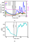 |
Fig. 1. Temporal evolution of (a) the spatially averaged absolute velocity components ⟨|vx(t)|⟩, ⟨|vy(t)|⟩, ⟨|vz(t)|⟩ and the ratio of free (Ef) to potential (Epot) energy (dashed magenta curve). The shaded region between t = 5.44 and 7 min (shown by two vertical dashed lines) represents the dynamical semi-equilibrium phase of the system, where ⟨|vy(t)|⟩≈19 km s−1, ⟨|vx(t)|⟩≈2.2 km s−1, ⟨|vz(t)|⟩≈5.4 km s−1, and Ef/Epot ≈ 2.1; and (b) the spatial average, |
where Bpot is the potential field extrapolated using the instantaneous By component at the base of the simulation domain (y = 0). The free energy Ef is the excess magnetic energy of the system from its corresponding potential field energy, given by
 (19)
(19)
Figure 1a shows that the value of Ef/Epot decreases sharply from 4.38 at the initial state to about 2.1 within ≈1 min, which remains constant until 7 min. The ratio Ef/Epot evolves toward the value 2 are probably changes in the magnetic energy that are observed in active regions during major flares (Gupta et al. 2021; Liu et al. 2023). To estimate the evolution of the LF, we calculated the spatial average of the parameter
 (20)
(20)
within the full simulation domain at each time step, as shown in Fig. 1b. This parameter represents the average relative angle formed by the current and the magnetic field, which is useful for determining the (not)force-free nature of the magnetic field. The initial value of the average angle between J and B is arcsin(α)≈18°, which reduces to ≈5° at t ≈ 5.44 min and has a minimum value of ≈4° at t = 7 min. This implies that the system achieves a nearly force-free state within minutes, and that the period between 5 and 7 min corresponds to a nearly semi-equilibrium phase. We explain below that the changes after t = 7 min are accompanied by large flux rope expulsions and flare-loop configurations, which again cause strong variations in velocity and LF. We first characterize the thermodynamical timescales for the nearly-force-free state between t = 5.44 and 7 min.
We estimated the characteristic timescales of background heating (τbh), radiative cooling (τrc), and field-aligned thermal conduction (τcon) at the start time of the dynamical semi-equilibrium state at t = 5.44 min, which were calculated by
 (21)
(21)
 (22)
(22)
 (23)
(23)
respectively, where ϵ = p/(γ − 1) is the internal energy density per unit volume. We calculated these characteristic timescales at each pixel of the simulation domain and obtained probability densities for them, as shown in Fig. 2. We note that τbh and τrc are more than 1000 s for the entire simulation domain (see Figs. 2a and b). To estimate the (magnetic field aligned) thermal conduction timescales τcon, we used a convolution filter using a uniform kernel of size 5 × 5 to smooth out the numerical discretization bias that arises in specific regions. We note that ≈76% of the domain corresponds to τcon > 100 s, and only 1.05% of the domain has less than 1 s. However, the dynamical semi-equilibrium phase of the system lasts for ≈93 s (the shaded region in Fig. 1a). Taking all these aspects into consideration, where the cooling and heating times are long and of similar magnitude, while thermal conduction quickly equilibrates temperatures along loops, we argue that the semi-equilibrium phase between 5.44 and 7 min is a relevant starting point for studying the later evolution of the system.
 |
Fig. 2. Discrete probability densities of the characteristic timescales of (a) background heating (τbh), (b) radiative cooling (τrc), and (c) thermal conduction (τcon) at t = 5.44 min. |
3.2. Development and eruption of flux ropes
The plasma density, temperature, LF, and MFL distribution of the semi-equilibrium state (at t = 5.44 min) are shown in the first column of Fig. 3. The MFLs resemble a coronal loop structure that is embedded in a bipolar magnetic field configuration. The evolution during the semi-equilibrium phase is slower than the violent initial phases, and the thermal processes cannot substantially modify the plasma during that phase, but it is not a pure equilibrium; rather, there is a small imbalance in the forces that leads to the events described in the following.
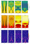 |
Fig. 3. Top row: spatial distribution of the plasma density for (a) the semi-equilibrium stage. Panels b–d show the different MFR eruption stages, where the overplotted solid curves represent the MFLs projected in the x − y plane. Middle row: same as in the top panel for temperature. Bottom row: distribution of the LF over the entire simulation domain, where the overplotted arrows represent the LF direction in the x − y plane. The saturation level of the color bar is taken up to 10−5 G2 cm−1 for a better visualization of the enhanced LF regions. Animations of the figures are available online (the height and width aspect ratio of the figures are not to scale). |
The LF tries to squeeze the magnetic arcades along the horizontal direction near the central region at x = 3.14 Mm (and also toward the periodic horizontal boundaries). This is clearly noticeable in Fig. 3i for the upper y ⪆ 7 Mm region. The squeezing of opposite-polarity field lines creates a localized region with small (about one Gauss) Bx and By components in the presence of the guide field Bz. This location leads to magnetic reconnection without a null point due to the presence of (uniform) resistivity (Priest & Démoulin 1995), which is shown in Figs. 3b and f. At around ≈7.66 min, a vertical current sheet (CS) forms in the central region between y ≈ 5 − 10 Mm, where the LF is enhanced, as shown in Fig. 3j. This CS region is heated to ≈4 MK, as shown in Fig. 3f. Due to reconnection in the CS plane, an erupting MFR is formed in the central region (see Figs. 3b or f). Due to the periodic condition at the horizontal boundaries, erupting MFRs are also formed later at ≈10 min at the side boundaries. This is shown in Figs. 3c and g. Further spontaneous reconnections lead to the formation of a second erupting flux rope in the central region at a lower height between y ≈ 0 − 5 Mm at around ≈12.67 min (see Figs. 3d and h), again accompanied by the formation of a CS underneath it. The temperature of this CS rises to ≈7 MK due to resistive heating. Cusp-like structures are formed beneath the vertical CSs, as shown in Figs. 3b, d, f, and h. This is similar to the classic CSHKP solar flare model (Carmichael 1964; Sturrock 1966; Hirayama 1974; Kopp & Pneuman 1976), where hot CSs are formed below erupting MFRs, and cusp-like magnetic structures form underneath CSs.
We show the flow patterns and the By distributions for the instants with clear central MFR eruptions in Figs. 4a and b. The location of reconnection in the bipolar magnetic structure is highlighted by the green ellipses in Figs. 4a and b, where the reconnection-driven inflows and outflows are evident. To appreciate the reconnection location, we quantify the distribution of vy and By shown in Fig. 4c and vx and Bx in Fig. 4d by taking a vertical cut at x = 3.14 Mm at t = 7.66 and 12.67 min, respectively. The regions where the outflow velocities flip directions are spatially colocated with the small (about one Gauss) magnetic field strength locations of Bx and By. The reconnection points are located in the central region (x = 3.14 Mm) at y ≈ 7.5 Mm for the first and y ≈ 3 Mm for the second (central) eruption. The maximum outflow velocities remain sub-Alfvénic, where the Alfvén velocity (va) was calculated based on the instantaneous local plasma density and magnetic field strength at a fixed location in the vicinity of the inflow side near the reconnection points. To estimate the reconnection rate at these locations, we considered the ratio of the magnitude of inflow velocity with respect to the instantaneous Alfvén velocity, ℳ = |vx/va|. The variation in |vx/va| in the central region is shown in Fig. 4d, where the reconnection rate is ≈0.05 for the first eruption and ≈0.15 for the second eruption near the reconnection points. This implies that the second eruption is more violent than the first.
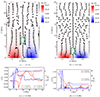 |
Fig. 4. Variation in the By field in the x − y plane shown at (a) t = 7.66 and (b) 12.67 min, where the overplotted black arrows represent the velocity field {vx, vy} in the x − y plane. The region inside the green ellipses (in panels a and b) contain the location of the reconnection points, where the plasma flows in and out due to reconnection (the height and width aspect ratio in the figures are not to scale). (c) vy and By distributions along y-direction at x = 3.14 Mm (which covers the location of the reconnection point). (d) Absolute velocity of the vx and Bx distributions in the y-direction at x = 3.14 Mm for the eruption phases. The velocities are scaled in units of instantaneous Alfvén speed (va). The solid and dashed curves in panels c and d represent the velocities and magnetic field strengths, respectively. |
This MFR eruption phase, where successive flux ropes are shed from the domain and escape through the top boundary, which is open to outflows, is energetically quantified in Fig. 5. The temporal distributions of the mean kinetic (KE) and magnetic (ME) energy densities, which are calculated by the spatial average of the entire simulation domain,
 (24)
(24)
 (25)
(25)
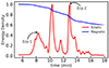 |
Fig. 5. Temporal evolution of (normalized) mean kinetic and magnetic energy densities during the eruption phases, where the black arrows represent the time when first (Erp 1) and second (Erp 2) eruptions from the central region have their peak KE densities. The other peaks between the two eruptions (Erp 1 and 2) show the signature due to eruptions from the side boundaries. |
are shown in Fig. 5. The KE exhibits strong peaks, two of which occur at ≈8 and 13 min and are associated with the first and second flux rope eruptions (marked Erp 1 and Erp 2, respectively) from the central region. The other peaks (one strong and the other relatively weaker) in between the two central eruptions are due to the secondary eruptions, which occur from the side boundaries (the first eruption is shown in Fig. 3c, and the second is not shown in the figure, but can be found in the associated animation that is available online). During the eruptions, the magnetic energy density decreases as free magnetic energy is converted into kinetic (and thermal) energy, and thus, we see the corresponding drop of the magnetic energy density. The drops are sharper during the peak eruption times when the KE density peaks, as shown in Fig. 5. Figures 3j and l show clear signature that the enhanced LF regions are colocated with the MFR locations of Figs. 3b and d, respectively.
To explore the dynamics of the eruptions themselves, we produced time-distance (TD) maps of the LF along a vertical cut at x = 3.14 Mm, as shown in Fig. 6. The choice of LF instead of density (or temperature) was made in this case because the LF maps show a clear signature of the MFR locations. To analyze the first eruption, we selected the temporal domain of the TD map between ≈6.3 to 9.33 min, as shown in Fig. 6a, where the enhanced LF region is tracked in the appropriate spatial and temporal domain, which corresponds to the flux rope eruption, and the eruption speed was estimated by calculating the slope (shown by the solid black line) of that region in the y − t plane. Similarly, for the second eruption (from the central region), we selected the temporal domain between ≈11.4 to 14.33 min, as shown in Fig. 6b, and tracked the enhanced LF regions corresponding to the eruption to estimate the eruption speeds. The speed of the first eruption is estimated to be ≈167 km s−1. For the second eruption, the flux rope speed is ≈441 km s−1 in the early phase and then decelerates to ≈217 km s−1. This agrees fairly well with observational evidence in solar flares, where the average rising velocity of the flux rope is reported ≈224 km s−1 (Yan et al. 2018). The density decreases in the ambient medium at around y ≈ 10 − 20 Mm after the first eruption (see Fig. 3d). The formation of the second flux rope also occurs at a lower height with a higher LF. These two effects make the eruption of the second MFR faster than that of the first MFR. This is also reflected in Fig. 5, which shows that the mean kinetic energy peak for the second eruption (Erp 2) exceeds the peak value of the first eruption (Erp 1).
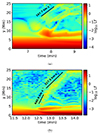 |
Fig. 6. Time-distance map of LF (in arbitrary units) along the vertical cut at x = 3.14 Mm. Panels a and b represent the time domain around the first and second flux rope eruption phases, respectively. The slope(s) at the selected part(s) in the maps is highlighted by the black lines to estimate the eruption speed of the flux ropes. |
3.3. Development of the thermal instability
As a consequence of post-eruption of the MFRs, the loop footpoints are heated by the combined effect of (field-aligned) thermal conduction, steady background heat (which is based on the initial density and temperature), and radiative cooling. This leads to the evaporation of plasma materials along the field lines. To investigate the flows of plasma materials, we estimated the velocity along the projection of the MFLs in the vertical XY plane, namely,  , as shown in Fig. 7. The eruptions with several MFRs that escape upward are followed by the flow of plasma materials along the field lines from the loop footpoints to the central loop top. These materials accumulate at the loop top, resulting in a gradual density enhancement. The radiative cooling rate in the optically thin corona, Hrc ∼ ρ2Λ(T), has derivatives
  , and
, and  at T ≈ 1 MK for the Λ(T) cooling curve we used in this model. The temperature at the loop top location (x, y) = (3.14, 4) Mm remains ∼1 MK between t ≈ 20 to 40 min (see Fig. 8, top panel); this implies that the radiative cooling rate at T ≈ 1 MK is more sensitive to the density perturbations than to those of temperature. The gradual mass accumulation at the loop top at x = 3.14 and around y = 4 Mm leads to an extended phase in which a thermal instability slowly sets in and causes a local condensation in the post-flare loop top. We followed the temporal evolution of temperature at four different locations at x = 1, 2, 3.14, and 4.7 Mm, all taken at the same height, namely y = 4 Mm, as shown in Fig. 8 (top panel). The temperature at these locations can reach values up to several million degrees during the eruption phase. The maximum temperature at (x, y) = (3.14, 4) Mm rises up to ≈7.6 MK at the CS location beneath the MFR during the second central eruption. After the second MFR eruption from the central region, there is a secondary eruption from the side boundaries (as shown in the animations associated with Fig. 3), which leaves the simulation domain from the top boundary at ≈38 min. About half an hour into our simulation, no further MFRs erupt, and the magnetic topology is seen to have changed into an arcade configuration with an overlying mostly horizontal field. The temperature evolution at the different selected x-values for y = 4 Mm show minor thermal fluctuations around a typical coronal 1 MK degree for t = 25 min onward (see the top panel of Fig. 8). These fluctuations are post-eruption effects. These perturbations settle down at ≈42 min. The temperature at the loop top location (x, y) = (3.14, 4) Mm gradually starts to fall down immediately after this (as shown by the green curve in the top panel of Fig. 8). This signals the gradual development of thermal instability at the post-eruption loop top. The temperature drop occurs as the cooling rate, which is a combination of optically thin radiation and field-aligned thermal conduction dominates the (steady but spatially varying) background heating given by Eq. (16). The temperature evolution at this (x, y) = (3.14, 4) Mm location in between t = 42 and 50 min represents the (nearly) linear decay phase of the temperature as shown in the bottom panel of Fig. 8. The temperature decay rate within this period is estimated to be ≈156 K s−1 by the slope marked by the dashed red line. The steady background heating rate at the loop top location is ≈4.33 × 10⁻³ erg cm−3 s−1. Figure 9 shows that the net heating rate due to conduction and background heat dominates the radiative cooling rate at the loop top location at the earlier stage of post eruption (between t ≈ 20 and 40 min). Later, radiative cooling gradually starts to dominate the heating from about t = 40 min onward, and at t = 64 min, the radiative cooling rate increases sharply, when a catastrophic thermal runaway process starts. This leads to a pressure drop at the loop top location compared to its surroundings (see Fig. 10g), which drives pressure-gradient flows into this location and leads to a rapid density enhancement and drop in temperature (shown by the right most vertical dashed line in the top panel of Fig. 8).
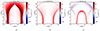 |
Fig. 7. Velocity map along the projected field lines in the vertical x − y plane, vfl, for three different times. |
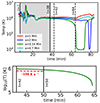 |
Fig. 8. Top panel: temperature evolution at four different horizontal locations at x = 1, 2, 3.14, and 4.7 Mm all at the same height y = 4 Mm. The shaded region between t = 7 to 38 min represents the eruption phase, where several MFRs leave the domain. The vertical dashed line at t = 42 min marks the time when the upper coronal part again settles down to around 1 MK. The dashed line at t = 64 min represents the onset of a thermal runaway process, which occurs first at the central x = 3.14 Mm location. Bottom panel: temperature evolution in the central (x, y) = (3.14, 4) Mm location. The temperature drops between t = 42 and 50 min with a decay rate of 156 K s−1, as represented by the dashed red line. |
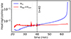 |
Fig. 9. Development of a thermal imbalance between heating and cooling at the loop top location (x, y) = (3.14, 4) Mm in the late phase of our simulation. The red curve denotes the heating rate due to thermal conduction (Hcon) and background heat (Hbgr), and the blue curve denotes the cooling rate due to radiation (Hrc). The units for all the quantities are in erg cm−3 s−1. The vertical dashed line marks the time after which the radiative cooling starts to dominate the heating due to conduction and background heat. |
3.4. Evolution of the coronal rain
The location of the first condensation seed that appears in the central loop top is shown in Fig. 10a. What happens next is shown visually in Fig. 10, which contains three rows for the density, temperature, and pressure, and three columns for t = 64.83 min, t = 80.10 min, and t = 83.01 min. Figures 10a and d show the maps of the density and temperature at t = 64.83 min. The density is enhanced up to ∼10−13 g cm−3, which is about 100 times more than the initial density (∼10−15 g cm−3), and the temperature drops to ∼10 kK, which is about 100 times lower than the initial temperature (1 MK). This thermal runaway process is only initiated at the magnetic loop top. The dips in the temperature curves in Fig. 8 (top panel) for both the (x, y) = (2, 4) and (3.14, 4) Mm locations (shown by the blue and green curves, respectively) show the temperature evolution at the fixed points and must be understood from the evolution, as shown in Figs. 10a–c. The condensation accumulates surrounding plasma, which is driven by the pressure gradient flows due to the pressure drop in the condensation site. The pressure is shown in the bottom panels of Fig. 10, where we note the inflow of matter from higher to lower gas pressure regions toward the condensation sites. Figure 10b shows that the loop top condensation has split into three isolated density clumps (or blobs), as marked by the white boxes. These clumps fall downward along the MFLs due to the combination of gravity and the LF, and they finally merge together again, as shown in Fig. 10c, at t = 83.01 min. These cool-condensed structures share similarities with the thermodynamic properties of coronal rain in the solar atmosphere, as observed by Müller et al. (2005), Antolin et al. (2015), Scullion et al. (2016), Mason et al. (2019), Şahin et al. (2023), and references therein, who reported a density and temperature of the rain clumps between ∼10−14 − 10−13 g cm−3, and ∼104 − 105 K, respectively.
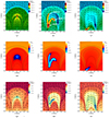 |
Fig. 10. Density (top panel), temperature (middle panel), and gas pressure (bottom panel) at different stages when the cool (∼104 K) and condensed (∼10−13 g cm−3) coronal rain forms. The location of three separated density blobs is marked by the white boxes in panel b. The overplotted solid black curves represent the MFLs, and the arrows in the bottom panels represent the velocity field {vx, vy} in the x − y plane. (a) t = 64.83 min. (b) t = 80.10 min. (c) t = 83.01 min. (d) t = 64.83 min. (e) t = 80.10 min. (f) t = 83.01 min. (g) t = 64.83 min. (h) t = 80.10 min. (i) t = 83.01 min. |
Figures 10d–f show that the cool (∼104 K) material is spatially colocated with the condensed structures in Figs. 10a–c. The corresponding radiative cooling losses are shown in Fig. 11. The maximum heat loss rate due to (optically thin) radiation in Fig. 11a is ≈9.06 × 10⁻¹ erg cm−3 s−1, which dominates the background heating of ≈4.33 × 10⁻³ erg cm−3 s−1. The maximum cooling rate increases at later times to 3.65 and 5.47 erg cm−3 s−1, as shown in Figs. 11b and c, respectively. The regions with high cooling rates correspond to the cool-condensed regions, as shown in the top and middle rows of Fig. 10. Our 2.5D assumption influences the appearance of the radiative cooling, showing the condensations as dark structures with bright edges, similar to the transition from a prominence to the coronal transition region (PCTR) obtained in other recent 2.5D simulations of coronal rain (Li et al. 2022).
 |
Fig. 11. Optically thin radiative cooling (RC) for the same time snapshots as in Fig. 10. (a) t = 64.83 min. (b) t = 80.1 min. (c) t = 83.01 min. |
The instantaneous maximum and minimum temperature evolution within the entire simulation domain is shown in Fig. 12a, which covers the entire period from eruptions to the late condensation stages. The minimum temperature distribution has two strong dips between ≈10 − 15 min. The first dip appears when the plasma blobs, which are denser than the surrounding medium, are trapped inside secondary erupting flux ropes from the side boundaries, which also correspond to a lower temperature than the background medium (see Figs. 3c and g). The second dip at about 14 min appears due to a trapped plasma blob inside the rope from the second central eruption (see Figs. 3d and h). The corresponding signatures are also evident in the red curve in Fig. 12a, which quantifies the instantaneous maximum density. The same figure later shows a sharp rise in this peak density (from ∼10−15 − 10−13 g cm−3) and a drop in the minimum temperature from ∼MK to ∼10 kK at ≈64 min. This signals the onset of the thermal runaway process to form the cool condensation at the loop top location (x, y) = (3.14, 4) Mm. This catastrophic drop in the (minimum) temperature occurs between ≈64 to 65 min, and the sudden temperature change during that short time interval is highlighted in Fig. 12b. The maximum rate of change in the temperature during this minute is ≈6.2 kK s−1. This catastrophic cooling rate agrees well with a 2.5D MHD simulation (Ruan et al. 2021) of a post-flare coronal rain scenario, where they found the average catastrophic cooling rate to be 9 kK s−1, and it agrees fairly well with observations for post-flare arcades (Scullion et al. 2016), where it is reported to be 22.7 kK s−1. The cooling rates are sometimes challenging to estimate in the observations because measurements of different spectral lines with different instruments and their responses are required to sample different parts of the flare. The details of the cooling curve prescription, Λ(T), also influence the condensation rates, as was shown in a purely coronal volume study that compared many popular cooling curves in Hermans & Keppens (2021). The temporal evolution of the rain mass and its area is shown in Fig. 13. We defined the localized condensations as coronal rain clumps when the density of these regions exceeded or was equal to a density threshold value that was ten times the maximum density of the initial state. To calculate the total rain mass at an instantaneous time, we collected all the cells with densities above the threshold, then multiplied the local densities with the area of the individual cells to obtain the mass per unit length of these individual cells, and we finally aggregated the quantity of all these cells. The evolution of the rain mass and area increases sharply from the onset time of thermal runaway at ≈64 min. This is also consistent with Fig. 12a because the catastrophic temperature drop occurs at the same time. The rain mass and area reach maximum values at ≈78.5 min. At about this time, the condensed region is separated into three individual density blobs (shown in Fig. 10b). Thereafter, rain mass and area decrease because the blobs start to coalesce while falling down, finally forming a single blob again (see Fig. 10c). The decrease in the rain mass and area after 79 min is also influenced by the fact that the smaller blobs are more easily evaporated again because they radiate energy in their PCTR and attain lower heights, where the background heating is higher. To track the motion of individual rain blobs, we used an automated method using binary masking from a python-based module, OpenCV2, to locate the instantaneous centroid locations of the density blobs. We started the tracking when it first separated into three blobs (around t ≈ 78 min) and continued until the end of the simulation when they merged together upon reaching the bottom (t ≈ 83.37 min). Blob 1 first falls down at the bottom, followed by blob 2, coalescing with blob 1, and finally, blob 3 falls down and merges with blobs 1 and 2 to form a single blob. The trajectories of the individual blobs are shown in Fig. 14a, where the falling blobs follow trajectories (nearly) along MFLs (see the animation associated with Fig. 3). Instantaneous vertical velocities of the individual blobs were calculated based on the instantaneous distance traversed along the vertical direction (y-direction) by the blobs between two consecutive simulation frames, taken at a temporal cadence of 4.29 s. The evolution of the falling rain velocity is shown in Fig. 14b, where we note that the velocity of the rain clumps is ≈1 − 40 km s−1. It increases as they accelerate while falling downward due to the combined effect of gravity, gas pressure gradients, and LF. This is clearly noticeable, especially for blobs 2 and 3 (in Fig. 14b), which obtain the maximum velocities when they reach the bottom just before coalescing with each other. They suddenly decelerate, which is due to our lower boundary condition and pressure gradient. The velocity of the downward falling rain clumps in our study agrees well with other simulation models. Examples include Fang et al. (2015), where the maximum velocity of the blobs in a rain shower is ≈60 km s−1, with most of the rain blobs having velocities ≈30 km s−1, and Li et al. (2022), where the velocity varies from a few to 120 km s−1. It also agrees reasonably well with the observations of Antolin et al. (2015) and Mason et al. (2019), who reported velocities of the rain clumps in the range of ≈50 − 100 km s−1.
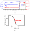 |
Fig. 12. (a) Time series of the instantaneous maximum and minimum temperature, and peak density. Panel b represents the temporal variation in the instantaneous minimum temperature, highlighting the catastrophic cooling phase, where the maximum cooling rate is estimated by the slope ≈ − 6200 K s−1 that is marked by the red line. |
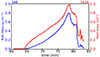 |
Fig. 13. Variation in the mass of the coronal rain and its area with time. |
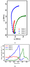 |
Fig. 14. Panel a shows the trajectories of the individual rain blobs in the x − y plane. Panel b shows the instantaneous vertical velocities of the individual falling rain clumps. |
4. Summary and discussion
We used a 2.5D resistive MHD simulation incorporating nonadiabatic effects of optically thin radiative cooling, field-aligned thermal conduction, and steady (but spatially varying) background heating to explore a series of flux rope eruptions, followed by gradual development of thermal instability, ultimately leading to a catastrophic cooling phase in the solar corona. The initial magnetic field configuration used in this simulation was motivated from Kumar et al. (2016), who studied the magnetic and dynamical properties of an erupting flux rope in an incompressible medium. We used the similar initial magnetic field prescription, but extended the study using a gravitationally stratified solar atmosphere in a compressible medium and the multithermal behavior in the solar corona.
The initial magnetic field was non-force-free, and its strength depended on three parameters, σ, γ (which is related to the shearing angle), and the field strength B0. These initial forces instantly induce flows that drive the plasma evolution. We showed that this imbalance transiently evolves to a more force-balanced, energetically settled semi-equilibrium stage after 5.44 min, which we used as a reference point for the rest of the simulation. The Lorentz force-driven flows cause convergence of plasma along the central axis and trigger magnetic reconnection, leading to flux rope formation and eruptions. The shearing angle of the magnetic arcades is also one of the important parameters for the formation of the flux ropes, and our simulation shows clear successive MFR formations with a shearing angle of  . To investigate the effect of a lower γ, we also ran the simulation up to ≈90 min with γ = 25°, keeping all the other parameters the same (not shown in our figures), and we note that there is no formation (and eruption) of flux ropes. Successive MFR eruptions are observed in a multiple flux rope system in a solar flare (Hou et al. 2018), where two consecutive double-decker flux rope eruptions occurred within an interval of five minutes due to strong shearing motions. This is very similar to our findings, where the interval between two (central) eruptions in our study is ≈4.9 min. Multiple MFR eruptions were also found in other simulations, such as in three-arcade configurations by Ding et al. (2006) in a resistive medium, and Soenen et al. (2009) in an ideal MHD regime. These studies showed homologous eruptions of multiple flux ropes from the same sites, which agrees with our findings, where the two MFRs are ejected from the central arcade region. However, the main focus of our study was to investigate the multiple eruption of flux ropes and the multithermal behavior in a localized domain in corona. This present setup is not motivated to portray a global MHD model, where it fits in the larger picture of CME evolutions, for instance, in a breakout scenario, and how the large-scale magnetic topology (at farther-out radii, i.e., in the top part of our simulation domain) evolves in solar corona. The use of periodic boundary condition at the side may be adopted meaningfully and is a standard procedure for a local-box simulation. Examples include Kumar et al. (2016), who studied the eruption, and Robinson et al. (2022), who studied the formation of a pre-flare flux rope in periodic side boundaries. In our simulation, the magnetic fields above the central arcade switch to a primary horizontal orientation when the eruptive flux ropes expand laterally, and this is mediated by the choice of periodic boundary condition at the sides. The horizontal magnetic field (Bx component) at the top part of the domain flips after each flux rope eruption. This is because the magnetic field (and mainly its horizontal component as introduced by the flux rope formations) due to each eruption dominates the remnant magnetic field of the previous eruption. However, we performed an additional simulation with a modified boundary condition, where we used a three-arcade system, and by extending the lateral and vertical domain of our simulation box (see Appendix A). This setup also showed a similar evolution: multiple eruptions of flux ropes from an initial not force-free setup, and the late stages of the post-flare arcade system that showed the formation of coronal condensation in a localized domain in corona. This clearly changes the way in which the eruptions proceed in the top part of the domain, but qualitatively, the evolution is the same in the two cases we simulated. We also note that the central flux ropes expand laterally while they erupt and create a horizontal field overlying the arcades. We admit that the details of the magnetic field topology in the top part of our domain, which drastically changes as successive flux ropes form and pass through, is not fully realistic in neither of the two simulated scenarios. We understand the importance of a more realistic setup, which needs to be handled better in future, where the actual radial expansion is allowed, for example, and the neighbouring magnetic flux evolutions are incorporated, such as for a full spherical model, and portray a large-scale (global) magnetic field of the solar corona. Nevertheless, our main findings (multiple eruptions and a post-flare multithermal evolution) is not affected by this. The temperature evolution at the CSs underneath the MFRs during the second central eruptions at (x, y) = (3.14, 4) Mm reaches ≈7 MK (from initially 1 MK). This high temperature would show clear brightenings in the soft X-ray band, which is relevant for flares.
The development of the thermal instability starts after the eruption of the flux ropes (see Fig. 8). It first leads to a linear decay of temperature followed by a later catastrophic temperature drop and formation of a condensation that evolves, splits, and falls down due to gravity. The cool material basically falls along the MFLs of the loop. The thermodynamic behavior of these cool-condensed structures agrees well with the coronal rain that is observed in the solar atmosphere. We note the formation of the condensation in the post-flare loop after ∼30 min of the last flux rope eruption. This timescale agrees with the observation for a C8.2 class post-flare coronal rain, where the time difference between the flare ribbon formation, and the first appearance of coronal rain in the post-flare loops is at ≈26 min (Scullion et al. 2016). The observational evidence for coronal rain formation at the loop top regions that fall downward along the MFLs is similar to what we find in our simulation. The condensation time scale also agrees reasonably well with an X2.1 class post-flare coronal rain observation, where the time gap between the peak phase of the flare and the first appearance of the condensation at the loop top is ≈50 min (Brooks et al. 2024). This indicates that our model closely agrees with actual post-flare coronal rain scenarios. The clumpy structure of the plasma blobs in our simulation is very much a feature of flare-driven rain, more so than in the quiescent (active region loop) rain, because the densities are much higher in the flare than in quiescent rain. The density and temperature structuring of the rain, forming a coronal sheath around the cooler and denser cores of the rain clumps we found in our study, is one of the unique aspects of the observations reported in Scullion et al. (2016). They detected the source of the formation of the rain first in the hotter and progressively later in the cooler extreme-ultraviolet (EUV) channels.
The role of resistivity η in our model is an important aspect in the formation of MFRs and the CSs they involve, but it also regulates current-driven Ohmic heating in all later phases where coronal condensations can form. The uniform resistivity we used in this model is η = 5 × 10⁻⁵ (in dimensionless units). To explore the effect of enhanced resistivity in the condensation process, we also ran the experiment with a higher value, η = 5 × 10⁻⁴ (in dimensionless units), keeping all the other parameters unchanged. No catastrophic cooling phase occurs in the system until 90 min. A more detailed parametric survey of γ, η, σ, and B0 for this model may be interesting to study in the future to understand the dependence of the eruption and condensation mechanisms on these parameters.
The maximum temperature in the upper half of the simulation domain reaches high values of up to ≈25 MK (see Fig. 12a). This is influenced by the fact that the successive MFRs also tend to evacuate this upper region, causing it to be heated more easily. The heating occurs due to our steady background heat prescription, which is based on the initial density and temperature values. The mass outflow from the top boundary due to the eruptions and the prescription of no inflow through it leads to a density drop in this upper region, and therefore, the background heat dominates the cooling, leading to a high temperature. The use of the background heat prescription in this model is motivated by the fact that it is exactly compensated for by the radiative cooling term in the initial state (there is no cooling due to thermal conduction at the initial stage because of our initial isothermal condition). Future extensions of this work should consider the detailed coupling to the lower chromosphere and photospheric regions. A localized heating prescription in the loop footpoints can also trigger thermal nonequilibrium (TNE) to promote and regulate the appearance of coronal condensations, as proposed by Antiochos & Klimchuk (1991). The recent study by Li et al. (2022) demonstrated the formation of coronal rain showers due to turbulent heating at the chromospheric footpoints. Our model can be advanced by extending the spatial domain from the chromosphere to the corona and incorporating localized heating at the loop footpoints. We plan to explore this in future simulations. This may produce a quasi-cyclic formation of a larger number of rain clumps or rain showers.
To conclude, our current model can reproduce the formation of post-flare coronal rain, where multiple flux rope eruptions occur from the same sites in the form of homologous ejections. It also sets the direction for a better understanding of the multithermal (∼10 kK–10 MK) behavior in the solar corona, which is important for revealing the broader aspect of coronal heating.
Movie
Movie 1 associated with Fig. 3 (dens_temp) Access Supplementary Material
Open source at: http://amrvac.org
More information can be found at https://docs.opencv.org/3.4/d3/dc0/groupimgprocshape.html
Acknowledgments
Data visualization and analysis were performed using https://visit-dav.github.io/visit-website/index.html and https://yt-project.org/. The authors thank the anonymous referee for the constructive suggestions, and also express their thanks to F. Moreno-Insertis, Eamon Scullion, Eric Priest, and Manuel Luna for the useful discussions and suggestions, that improved the manuscript considerably. S.S. and A.P. acknowledge support by the European Research Council through the Synergy Grant #810218 (“The Whole Sun”, ERC-2018-SyG). S.S. and R.K. acknowledge support by the C1 project TRACESpace funded by KU Leuven, the ERC grant agreement 833251 Prominent ERC-ADG 2018, and FWO grant G0B4521N. R.K. acknowledges ISSI in Bern, Team project #545. A.P. would like to acknowledge the support from the Research Council of Norway through its Centres of Excellence scheme, project number 262622. The computational resources and services used in this work were provided by the VSC (Flemish Supercomputer Center), funded by the Research Foundation Flanders (FWO) and the Flemish Government – department EWI; La Palma supercomputer, provided by Instituto de Astrofísica de Canarias (IAC).
References
- Alfvén, H. 1942, Nature, 150, 405 [Google Scholar]
- Amari, T., Luciani, J. F., Aly, J. J., Mikic, Z., & Linker, J. 2003, ApJ, 585, 1073 [NASA ADS] [CrossRef] [Google Scholar]
- Antiochos, S. K. 1980, ApJ, 241, 385 [NASA ADS] [CrossRef] [Google Scholar]
- Antiochos, S. K., & Klimchuk, J. A. 1991, ApJ, 378, 372 [Google Scholar]
- Antiochos, S. K., & Sturrock, P. A. 1978, ApJ, 220, 1137 [NASA ADS] [CrossRef] [Google Scholar]
- Antiochos, S. K., DeVore, C. R., & Klimchuk, J. A. 1999, ApJ, 510, 485 [Google Scholar]
- Antolin, P., Vissers, G., Pereira, T. M. D., Rouppe van der Voort, L., & Scullion, E. 2015, ApJ, 806, 81 [Google Scholar]
- Aschwanden, M. J. 2004, Physics of the Solar Corona. An Introduction (Berlin: Springer-Verlag) [Google Scholar]
- Aschwanden, M. J., & Alexander, D. 2001, Sol. Phys., 204, 91 [NASA ADS] [CrossRef] [Google Scholar]
- Aulanier, G., Janvier, M., & Schmieder, B. 2012, A&A, 543, A110 [NASA ADS] [CrossRef] [EDP Sciences] [Google Scholar]
- Brooks, D. H., Warren, H. P., & Landi, E. 2021, ApJ, 915, L24 [NASA ADS] [CrossRef] [Google Scholar]
- Brooks, D. H., Reep, J. W., Ugarte-Urra, I., Unverferth, J. E., & Warren, H. P. 2024, ApJ, 962, 105 [NASA ADS] [CrossRef] [Google Scholar]
- Bruzek, A. 1964, ApJ, 140, 746 [NASA ADS] [CrossRef] [Google Scholar]
- Cargill, P. J., Mariska, J. T., & Antiochos, S. K. 1995, ApJ, 439, 1034 [NASA ADS] [CrossRef] [Google Scholar]
- Carmichael, H. 1964, NASA Spec. Publ., 50, 451 [NASA ADS] [Google Scholar]
- Chen, P. F. 2011, Liv. Rev. Sol. Phys., 8, 1 [Google Scholar]
- Claes, N., & Keppens, R. 2019, A&A, 624, A96 [NASA ADS] [CrossRef] [EDP Sciences] [Google Scholar]
- Claes, N., Keppens, R., & Xia, C. 2020, A&A, 636, A112 [EDP Sciences] [Google Scholar]
- Colgan, J., Abdallah, J., Sherrill, M. E., et al. 2008, ApJ, 689, 585 [NASA ADS] [CrossRef] [Google Scholar]
- Dalgarno, A., & McCray, R. A. 1972, ARA&A, 10, 375 [Google Scholar]
- Ding, J. Y., Hu, Y. Q., & Wang, J. X. 2006, Sol. Phys., 235, 223 [NASA ADS] [CrossRef] [Google Scholar]
- Druett, M. K., Ruan, W., & Keppens, R. 2023, Sol. Phys., 298, 134 [NASA ADS] [CrossRef] [Google Scholar]
- Fan, Y., & Gibson, S. E. 2007, ApJ, 668, 1232 [Google Scholar]
- Fang, X., Xia, C., Keppens, R., & Van Doorsselaere, T. 2015, ApJ, 807, 142 [NASA ADS] [CrossRef] [Google Scholar]
- Fleishman, G. D., Gary, D. E., Chen, B., et al. 2020, Science, 367, 278 [NASA ADS] [CrossRef] [Google Scholar]
- Froment, C., Auchère, F., Bocchialini, K., et al. 2015, ApJ, 807, 158 [NASA ADS] [CrossRef] [Google Scholar]
- Froment, C., Auchère, F., Aulanier, G., et al. 2017, ApJ, 835, 272 [Google Scholar]
- Gupta, M., Thalmann, J. K., & Veronig, A. M. 2021, A&A, 653, A69 [NASA ADS] [CrossRef] [EDP Sciences] [Google Scholar]
- He, W., Hu, Q., Jiang, C., Qiu, J., & Prasad, A. 2022, ApJ, 934, 103 [NASA ADS] [CrossRef] [Google Scholar]
- Hermans, J., & Keppens, R. 2021, A&A, 655, A36 [NASA ADS] [CrossRef] [EDP Sciences] [Google Scholar]
- Hirayama, T. 1974, Sol. Phys., 34, 323 [Google Scholar]
- Hou, Y. J., Zhang, J., Li, T., Yang, S. H., & Li, X. H. 2018, A&A, 619, A100 [NASA ADS] [CrossRef] [EDP Sciences] [Google Scholar]
- Jenkins, J. M., & Keppens, R. 2021, A&A, 646, A134 [NASA ADS] [CrossRef] [EDP Sciences] [Google Scholar]
- Keppens, R., Nool, M., Tóth, G., & Goedbloed, J. P. 2003, Comput. Phys. Commun., 153, 317 [Google Scholar]
- Keppens, R., Meliani, Z., van Marle, A. J., et al. 2012, J. Comput. Phys., 231, 718 [Google Scholar]
- Keppens, R., Teunissen, J., Xia, C., & Porth, O. 2021, Comput. Math. Appl., 81, 316 [Google Scholar]
- Keppens, R., Popescu Braileanu, B., Zhou, Y., et al. 2023, A&A, 673, A66 [NASA ADS] [CrossRef] [EDP Sciences] [Google Scholar]
- Kliem, B., & Török, T. 2006, Phys. Rev. Lett., 96, 255002 [Google Scholar]
- Kopp, R. A., & Pneuman, G. W. 1976, Sol. Phys., 50, 85 [Google Scholar]
- Kumar, S., Bhattacharyya, R., Joshi, B., & Smolarkiewicz, P. K. 2016, ApJ, 830, 80 [NASA ADS] [CrossRef] [Google Scholar]
- Li, X., Keppens, R., & Zhou, Y. 2022, ApJ, 926, 216 [NASA ADS] [CrossRef] [Google Scholar]
- Liu, W., De Pontieu, B., Vial, J.-C., et al. 2015, ApJ, 803, 85 [NASA ADS] [CrossRef] [Google Scholar]
- Liu, Y., Welsch, B. T., Valori, G., et al. 2023, ApJ, 942, 27 [NASA ADS] [CrossRef] [Google Scholar]
- Lohner, R. 1987, Comput. Meth. Appl. Mech. Eng., 61, 323 [CrossRef] [Google Scholar]
- Mason, E. I., Antiochos, S. K., & Viall, N. M. 2019, ApJ, 874, L33 [Google Scholar]
- Müller, D. A. N., de Groof, A., de Pontieu, B., & Hansteen, V. H. 2005, in Chromospheric and Coronal Magnetic Fields, eds. D. E. Innes, A. Lagg, & S. A. Solanki, ESA Spec. Publ., 596, 37.1 [Google Scholar]
- Porth, O., Xia, C., Hendrix, T., Moschou, S. P., & Keppens, R. 2014, ApJS, 214, 4 [Google Scholar]
- Priest, E. 2014, Magnetohydrodynamics of the Sun (Cambridge: Cambridge University Press) [Google Scholar]
- Priest, E. R., & Démoulin, P. 1995, J. Geophys. Res., 100, 23443 [NASA ADS] [CrossRef] [Google Scholar]
- Robinson, R. A., Carlsson, M., & Aulanier, G. 2022, A&A, 668, A177 [NASA ADS] [CrossRef] [EDP Sciences] [Google Scholar]
- Ruan, W., Xia, C., & Keppens, R. 2020, ApJ, 896, 97 [NASA ADS] [CrossRef] [Google Scholar]
- Ruan, W., Zhou, Y., & Keppens, R. 2021, ApJ, 920, L15 [NASA ADS] [CrossRef] [Google Scholar]
- Şahin, S., Antolin, P., Froment, C., & Schad, T. A. 2023, ApJ, 950, 171 [CrossRef] [Google Scholar]
- Scullion, E., Rouppe van der Voort, L., Wedemeyer, S., & Antolin, P. 2014, ApJ, 797, 36 [Google Scholar]
- Scullion, E., Rouppe van der Voort, L., Antolin, P., et al. 2016, ApJ, 833, 184 [NASA ADS] [CrossRef] [Google Scholar]
- Sen, S., & Keppens, R. 2022, A&A, 666, A28 [NASA ADS] [CrossRef] [EDP Sciences] [Google Scholar]
- Sen, S., Jenkins, J., & Keppens, R. 2023, A&A, 678, A132 [NASA ADS] [CrossRef] [EDP Sciences] [Google Scholar]
- Soenen, A., Zuccarello, F. P., Jacobs, C., et al. 2009, A&A, 501, 1123 [NASA ADS] [CrossRef] [EDP Sciences] [Google Scholar]
- Sturrock, P. A. 1966, Nature, 211, 695 [Google Scholar]
- van Leer, B. 1974, J. Comput. Phys., 14, 361 [NASA ADS] [CrossRef] [Google Scholar]
- Xia, C., Keppens, R., & Fang, X. 2017, A&A, 603, A42 [NASA ADS] [CrossRef] [EDP Sciences] [Google Scholar]
- Xia, C., Teunissen, J., El Mellah, I., Chané, E., & Keppens, R. 2018, ApJS, 234, 30 [Google Scholar]
- Yan, X. L., Yang, L. H., Xue, Z. K., et al. 2018, ApJ, 853, L18 [Google Scholar]
- Zhao, X., Xia, C., Keppens, R., & Gan, W. 2017, ApJ, 841, 106 [Google Scholar]
Appendix A: Evolution of the system with a modified setup
We performed an additional simulation with a modified setup, where we used a three-arcade system by extending the lateral domain of our boundary from x = 0 to 3π Mm (9.42 Mm) and the top boundary from y = 0 to 40 Mm. We used the highest resolution of 65 km and 54 km in the x and y directions, respectively. We modified the side boundary condition from periodic to the prescription according to Jenkins & Keppens (2021), where the density and pressure are symmetric; vx, vy, vz are antisymmetric, symmetric, and antisymmetric, respectively; Bx, By, and Bz are antisymmetric, symmetric, and antisymmetric, respectively, at the left and right boundaries. The top and bottom boundary conditions followed the same prescription as described in Section 2. The density, temperature, and MFL evolution for the eruptions are shown in Figure A.1. We note the formation of multiple flux ropes from the central arcade, which expand laterally while they erupt, and create horizontal field overlying the arcades. The magnetic field topology above the arcades changes drastically as successive flux ropes form and pass through. Finally, we note the formation of coronal condensation at the central loop top at t ≈ 33 min, which splits into different rain blobs and fall down, as shown in Figure A.2. This condensation timescale is earlier than in the other setup (which is at about 64 min). This difference in timescale appears due to the initial magnetic field structure with three arcades, the modified boundary condition at the side, the different spatial domain, and the spatial resolution.
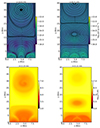 |
Fig. A.1. Spatial distribution of the plasma density (top panel) and temperature (bottom panel) for t = 13.23, and 21.11 min. The overplotted solid curves represent the MFLs projected in the x − y plane (height and width aspect ratio of the figures are not to scale). |
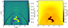 |
Fig. A.2. Spatial distribution of density (left) and temperature (right) distribution at t = 35.78 min, showing the splitting of the coronal rain blobs that forms at the loop top. The overplotted black curves represent the MFLs projected in the x − y plane. |
All Figures
|
Fig. 1. Temporal evolution of (a) the spatially averaged absolute velocity components ⟨|vx(t)|⟩, ⟨|vy(t)|⟩, ⟨|vz(t)|⟩ and the ratio of free (Ef) to potential (Epot) energy (dashed magenta curve). The shaded region between t = 5.44 and 7 min (shown by two vertical dashed lines) represents the dynamical semi-equilibrium phase of the system, where ⟨|vy(t)|⟩≈19 km s−1, ⟨|vx(t)|⟩≈2.2 km s−1, ⟨|vz(t)|⟩≈5.4 km s−1, and Ef/Epot ≈ 2.1; and (b) the spatial average, |
| In the text | |
|
Fig. 2. Discrete probability densities of the characteristic timescales of (a) background heating (τbh), (b) radiative cooling (τrc), and (c) thermal conduction (τcon) at t = 5.44 min. |
| In the text | |
|
Fig. 3. Top row: spatial distribution of the plasma density for (a) the semi-equilibrium stage. Panels b–d show the different MFR eruption stages, where the overplotted solid curves represent the MFLs projected in the x − y plane. Middle row: same as in the top panel for temperature. Bottom row: distribution of the LF over the entire simulation domain, where the overplotted arrows represent the LF direction in the x − y plane. The saturation level of the color bar is taken up to 10−5 G2 cm−1 for a better visualization of the enhanced LF regions. Animations of the figures are available online (the height and width aspect ratio of the figures are not to scale). |
| In the text | |
|
Fig. 4. Variation in the By field in the x − y plane shown at (a) t = 7.66 and (b) 12.67 min, where the overplotted black arrows represent the velocity field {vx, vy} in the x − y plane. The region inside the green ellipses (in panels a and b) contain the location of the reconnection points, where the plasma flows in and out due to reconnection (the height and width aspect ratio in the figures are not to scale). (c) vy and By distributions along y-direction at x = 3.14 Mm (which covers the location of the reconnection point). (d) Absolute velocity of the vx and Bx distributions in the y-direction at x = 3.14 Mm for the eruption phases. The velocities are scaled in units of instantaneous Alfvén speed (va). The solid and dashed curves in panels c and d represent the velocities and magnetic field strengths, respectively. |
| In the text | |
|
Fig. 5. Temporal evolution of (normalized) mean kinetic and magnetic energy densities during the eruption phases, where the black arrows represent the time when first (Erp 1) and second (Erp 2) eruptions from the central region have their peak KE densities. The other peaks between the two eruptions (Erp 1 and 2) show the signature due to eruptions from the side boundaries. |
| In the text | |
|
Fig. 6. Time-distance map of LF (in arbitrary units) along the vertical cut at x = 3.14 Mm. Panels a and b represent the time domain around the first and second flux rope eruption phases, respectively. The slope(s) at the selected part(s) in the maps is highlighted by the black lines to estimate the eruption speed of the flux ropes. |
| In the text | |
|
Fig. 7. Velocity map along the projected field lines in the vertical x − y plane, vfl, for three different times. |
| In the text | |
|
Fig. 8. Top panel: temperature evolution at four different horizontal locations at x = 1, 2, 3.14, and 4.7 Mm all at the same height y = 4 Mm. The shaded region between t = 7 to 38 min represents the eruption phase, where several MFRs leave the domain. The vertical dashed line at t = 42 min marks the time when the upper coronal part again settles down to around 1 MK. The dashed line at t = 64 min represents the onset of a thermal runaway process, which occurs first at the central x = 3.14 Mm location. Bottom panel: temperature evolution in the central (x, y) = (3.14, 4) Mm location. The temperature drops between t = 42 and 50 min with a decay rate of 156 K s−1, as represented by the dashed red line. |
| In the text | |
|
Fig. 9. Development of a thermal imbalance between heating and cooling at the loop top location (x, y) = (3.14, 4) Mm in the late phase of our simulation. The red curve denotes the heating rate due to thermal conduction (Hcon) and background heat (Hbgr), and the blue curve denotes the cooling rate due to radiation (Hrc). The units for all the quantities are in erg cm−3 s−1. The vertical dashed line marks the time after which the radiative cooling starts to dominate the heating due to conduction and background heat. |
| In the text | |
|
Fig. 10. Density (top panel), temperature (middle panel), and gas pressure (bottom panel) at different stages when the cool (∼104 K) and condensed (∼10−13 g cm−3) coronal rain forms. The location of three separated density blobs is marked by the white boxes in panel b. The overplotted solid black curves represent the MFLs, and the arrows in the bottom panels represent the velocity field {vx, vy} in the x − y plane. (a) t = 64.83 min. (b) t = 80.10 min. (c) t = 83.01 min. (d) t = 64.83 min. (e) t = 80.10 min. (f) t = 83.01 min. (g) t = 64.83 min. (h) t = 80.10 min. (i) t = 83.01 min. |
| In the text | |
|
Fig. 11. Optically thin radiative cooling (RC) for the same time snapshots as in Fig. 10. (a) t = 64.83 min. (b) t = 80.1 min. (c) t = 83.01 min. |
| In the text | |
|
Fig. 12. (a) Time series of the instantaneous maximum and minimum temperature, and peak density. Panel b represents the temporal variation in the instantaneous minimum temperature, highlighting the catastrophic cooling phase, where the maximum cooling rate is estimated by the slope ≈ − 6200 K s−1 that is marked by the red line. |
| In the text | |
|
Fig. 13. Variation in the mass of the coronal rain and its area with time. |
| In the text | |
|
Fig. 14. Panel a shows the trajectories of the individual rain blobs in the x − y plane. Panel b shows the instantaneous vertical velocities of the individual falling rain clumps. |
| In the text | |
|
Fig. A.1. Spatial distribution of the plasma density (top panel) and temperature (bottom panel) for t = 13.23, and 21.11 min. The overplotted solid curves represent the MFLs projected in the x − y plane (height and width aspect ratio of the figures are not to scale). |
| In the text | |
|
Fig. A.2. Spatial distribution of density (left) and temperature (right) distribution at t = 35.78 min, showing the splitting of the coronal rain blobs that forms at the loop top. The overplotted black curves represent the MFLs projected in the x − y plane. |
| In the text | |
Current usage metrics show cumulative count of Article Views (full-text article views including HTML views, PDF and ePub downloads, according to the available data) and Abstracts Views on Vision4Press platform.
Data correspond to usage on the plateform after 2015. The current usage metrics is available 48-96 hours after online publication and is updated daily on week days.
Initial download of the metrics may take a while.