| Issue |
A&A
Volume 695, March 2025
|
|
|---|---|---|
| Article Number | A1 | |
| Number of page(s) | 11 | |
| Section | The Sun and the Heliosphere | |
| DOI | https://doi.org/10.1051/0004-6361/202451543 | |
| Published online | 25 February 2025 | |
The role of the external toroidal magnetic field on the large-angle rotation of magnetic flux ropes
1
School of Astronomy and Space Science and Key Laboratory of Modern Astronomy and Astrophysics, Nanjing University, Nanjing 210023, China
2
Centre for Mathematical Plasma Astrophysics, Department of Mathematics, KU Leuven, Celestijnenlaan 200B, B-3001 Leuven, Belgium
⋆ Corresponding author; This email address is being protected from spambots. You need JavaScript enabled to view it.
Received:
17
July
2024
Accepted:
17
January
2025
Abstract
Context. It is accepted that magnetic flux ropes might exhibit large-angle rotation in magnetic configurations, including strong external toroidal magnetic fields. The specific mechanisms leading to rotation still remain elusive, however.
Aims. We examine the mechanisms by which the external toroidal magnetic field facilitates the flux-rope rotation, and we explore potential alternative rotation mechanisms beyond the effects of sheared fields and kink instability.
Methods. We performed three-dimensional magnetohydrodynamic simulations to model the eruption of magnetic flux ropes in a magnetic configuration with and without external toroidal magnetic fields. We compared the morphology, the dynamics, the magnetic topology, and the Lorentz force acting on the flux rope.
Results. The behavior of flux ropes in two simulations is significantly different. The flux rope that evolved without external toroidal fields successfully erupted was accompanied by minor rotation, and the flux rope that evolved with an external toroidal field was confined by large-angle rotation. The evolution of the magnetic topology, the Lorentz force, and the torque showed distinctive patterns in each scenario. Furthermore, the flux ropes in both simulations displayed observable signs of a drifting footpoint.
Conclusions. We reveal that external toroidal magnetic fields facilitate the flux-rope rotation, which in turn releases initial twists and amplifies the lateral Lorentz force exerted on the flux rope. The slipping magnetic reconnection between the flux-rope field lines and sheared-arcade field lines can contribute to the rotation, as does the lateral Lorentz force and the kink instability, which is determined by the initial twist number. Moreover, our result suggests that the initial twist of the flux rope cannot determine the rotation angle. The rotation angle of the flux rope does not strictly increase with the initial twist. The rapid release of the twist number necessitates external toroidal magnetic fields.
Key words: Sun: coronal mass ejections (CMEs) / Sun: filaments / prominences / Sun: magnetic fields
© The Authors 2025
 Open Access article, published by EDP Sciences, under the terms of the Creative Commons Attribution License (https://creativecommons.org/licenses/by/4.0), which permits unrestricted use, distribution, and reproduction in any medium, provided the original work is properly cited.
This article is published in open access under the Subscribe to Open model. This email address is being protected from spambots. You need JavaScript enabled to view it. to support open access publication.
1. Introduction
The solar atmosphere is not as calm as expected. Various violent eruptions occur frequently in the corona. One common and remarkable phenomenon is a filament eruption. When nonpotential coronal magnetic fields, such as magnetic flux ropes (MFRs) or sheared arcades, which host cold and dense filament materials, are disturbed beyond the threshold of an magnetohydrodynamics (MHD) instability, their ejection is initiated (Chen 2011). When this ejected magnetized plasma successfully escapes the restriction of the solar corona, it generates the largest and strongest eruptions in the Solar System, namely, coronal mass ejections (CMEs). When CMEs propagate near the Earth, they may cause disturbances in the geomagnetic environment and thus lead to space weather events. The hazard level induced by CMEs is highly related to their magnetic field orientations and propagation speeds (Srivastava & Venkatakrishnan 2004; Wilson 1987; Tsurutani et al. 1988). Concretely, faster CMEs carrying stronger southward magnetic field components frequently lead to more intense geomagnetic storms (Wilson 1987; Tsurutani et al. 1988). Some works have found that the magnetic fields of CMEs that were detected near the Earth have the same orientation as their precursors (e.g., filaments) in the solar source regions (Manchester et al. 2017). However, the magnetic field orientation of CMEs upon arrival at Earth is greatly influenced by their nonradial motions in the eruption and propagation process (Vourlidas et al. 2011; Lynch et al. 2009; Yurchyshyn et al. 2009). One significant factor is the rotation during the CME eruption. Kay et al. (2017) reconstructed the trajectory of seven CMEs from one active region during four-day eruptions and found that most of the rotation occurred below 2 solar radii. Many theoretical and numerical works have shown that rotations of more than 50 degrees during CMEs preferentially occur in the low corona (Fan & Gibson 2004; Lynch et al. 2009; Török et al. 2004). Additionally, some previous works also pointed out that many failed eruptions were associated with significant rotation (Zhou et al. 2019). Therefore, it is highly significant to study the rotation of filaments when the generation of a CME and its resulting space-weather effects are to be predicted. Three candidates that are thought to cause the large-angle rotation of CME MFRs were reported so far: (1) The release of twists of CME MFRs, which is often considered to be associated with the kink instability (Török & Kliem 2005); (2) the lateral Lorentz force acting upon the CME MFRs, which results from the external magnetic fields (Isenberg & Forbes 2007); and (3) the magnetic reconnection in which CME MFRs take part during the eruption (Török & Kliem 2005; Williams et al. 2005; Guo et al. 2023). However, quantifying the contributions of these three mechanisms to the large-angle rotation of CME MFRs remains elusive.
It is well accepted that the helical kink instability (Török & Kliem 2005) and lateral Lorentz force (Isenberg & Forbes 2007) are two of the most prevalent mechanisms that can cause the large-angle rotation of CME MFRs. The former determines the trigger and rotation angle of an MFR by examining the twist number of the flux rope. In this scenario, the rotation of a CME MFR results from the transformation of the twist to a writhe due to helicity conservation. This means that the initial twist of an MFR, as a a reservoir, directly determines the potential rotation angle in its eruption process. Additionally, the kink instability is also closely related to the ultimate fate of an eruption, namely, it determines whether the eruption is confined or successful. When the MFR does not meet the triggering conditions of a kink instability, even when the overlying strapping fields decay fast enough and meet the conditions for a torus instability (Kliem & Török 2006), it may still experience a failed eruption (Myers et al. 2015). Regarding effects of the lateral Lorentz force in inducing the MFR rotation, the essential physical theories were first mentioned by Isenberg & Forbes (2007) as an inspiration. Therefore, it is speculated that an MFR could be subjected to a lateral force and rotate when passing through toroidal-field-dominated external magnetic structures. Subsequently, Kliem et al. (2012) conducted a parameter survey of the height and rotation angle evolution of MFRs under the external toroidal field (referred to as the external shear-field component in the paper). The authors pointed out that external toroidal fields contribute more to the large-angle rotation than the release of the MFR twist. Recently, an increasing number of works have realized that external toroidal magnetic fields play an important role in the dynamics of MFRs, both for the rotation and for the failed eruption (Zhang et al. 2024; Wang et al. 2023; Jiang et al. 2023; Guo et al. 2024). In this paper, we aim to quantify the interaction of external toroidal magnetic fields with MFRs. We determine how these fields promote rotation or prevent eruption with the aid of simulations.
Furthermore, magnetic reconnection can also cause the rotation of CME MFRs. Magnetic reconnection is a common way of energy release on the Sun. It releases substantial magnetic energy in a short period of time by changing the connectivity of the magnetic field in the dissipation zone of a current sheet (Chen et al. 1999). The standard two-dimensional (2D) flare model (CSHKP model; Carmichael (1964), Sturrock (1966), Hirayama (1974), Kopp & Pneuman (1976)) describes that reconnection outflows and magnetic tension force play a significant role in driving the ascent of the above MFRs. Although this 2D CSHKP model captures certain critical observational characteristics, the flares in observations frequently exhibit many 3D phenomena, such as the drifting of the MFR footpoints, saddle-like flare loops, J-shaped ribbons, and the decrease in toroidal fluxes. In conjunction with these observational characteristic insights, a 3D standard flare model within the context of slipping magnetic reconnection was proposed by Janvier et al. (2014), Aulanier & Dudík (2019). In this model, slipping magnetic reconnection occurs in the hyperbolic flux tube and can change the magnetic topology of the CME flux rope. On the one hand, this reconnection can result in the drifting of the flux-rope footpoints along QSLs. On the other hand, the reconnection between flux-rope field lines and sheared arcades (ar − rf reconnection) can change the connectivity of the flux-rope field lines, thereby leading to the rotation in observations. As a result, an underlying relation between the drifting of the flux-rope footpoints and its rotation is expected.
We aim to quantify the contributions of the aforementioned candidates to large-angle rotation by addressing the following three problems: (1) We elucidate the role of external overlying toroidal magnetic fields in inducing the rotation of an MFR. (2) We investigate the potential influence of slipping reconnection on this rotational behavior. (3) We finally assess whether the initial twist can be estimated from the observed flux-rope rotation angle. Following this line of problems, we briefly introduce our simulation setups in Sect. 2, and we then present our results with particular emphasis on the differences between a successful eruption simulation (SES) and a failed eruption simulation (FES) in Sect. 3. Finally, we discuss the above questions in Sect. 4 and provide our conclusions in Sect. 5.
2. Numerical setup
As delineated in Sect. 1, the external toroidal magnetic field facilitates the large-angle rotation of CME MFRs. To explore how external toroidal magnetic fields influence the dynamics of CME MFRs, we conducted two MHD simulations of solar eruptions including a preexisting MFR and contrasted scenarios with and without the external toroidal field. As a result, a comparative analysis of the evolution of flux-rope morphology and associated physical parameters was undertaken.
First, we established the framework of a coordinate system for numerical computations of the MHD equations. We applied Cartesian coordinates, and the solar surface corresponded to the xOy plane in the numerical simulations. The initial condition of the magnetic field was based on the TDm model (Titov et al. 2014), which is constructed based on the regularized Biot–Savart laws (RBSL; Titov et al. 2018). In the FES case, we also added two magnetic charges located on the y -axis to provide the external toroidal magnetic fields. In the two simulation cases, the major and minor radii of the flux rope were 30 Mm and 12 Mm, respectively. The detailed parameters of the magnetic charges and flux ropes are listed in Table 1. Fig. 1 presents the initial magnetic configurations of cases SES and FES, where the external magnetic field lines in the FES case are elongated in the toroidal direction.
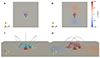 |
Fig. 1. Initial magnetic field configurations. (a, c) MFR and external field lines of SES in top and side views, (b, d) and those of FES in the same views. |
Parameters of external field charges and flux ropes in the initial setups of the two simulations.
An isothermal MHD model was employed to conduct the following simulations, described by the following governing equations:
 (1)
(1)
 (2)
(2)
 (3)
(3)
where the total pressure ptot = cadiabργ + B2/(2μ0), the adiabatic constant cadiab = 1.4 × 10¹⁴ erg g−1, the polytropic index γ = 1 (which ensures an isothermal model), the vacuum permeability μ0 = 4π × 10−9 H cm−1, the identity tensor I and the gravitational acceleration g = −k g⊙ r⊙2/(r⊙ + z)2ez, in which the gravitational acceleration g⊙ = 2.74 × 104 cm s−2 on the solar surface, and the solar radius r⊙ = 695.5 Mm. We note that in our model, gravity g is modified with a constant ratio k = 1.8 to remain low β in weak magnetic regions (Jiang et al. 2021). Additionally, the initial density was derived from an isothermal atmosphere of 106 K. We first assumed a reference density ρ0 = 2.34 × 10⁻¹⁵ g cm−3 at z = 0. Then, we combined the ideal gas law with the condition of hydrostatic equilibrium ∇p = −ρg and derived the initial density distribution.
The aforementioned equations were solved numerically within a Cartesian coordinate system, employing the code called message passing interface adaptive mesh refinement versatile advection code (MPI-AMRVAC; Xia et al. 2018; Keppens et al. 2023). The simulation domain was [xmin, xmax]×[ymin, ymax]×[zmin, zmax]=[−180, 180]×[−180, 180]×[0, 360] Mm. A three-level adaptive mesh refinement was applied with a basic mesh grid of 60 × 60 × 60. To maintain numerical stability, the constrained-transport (CT) method on staggered grids was employed, effectively suppressing divergence to machine accuracy (⟨|fi|⟩ ∼ 10−16, see Wheatland et al. (2000) for this metric) during the simulations. A line-tied bottom condition was implemented by ensuring a zero horizontal electric field. Additionally, the lateral and top boundaries were open with zero-gradient extrapolation. For both cases, we saved the data every t0 = 21 s for the following analysis.
3. Numerical results
3.1. Evolution of the magnetic field
Figure 2 shows the overall evolution for the SES and FES cases. The magnetic field lines are traced either from initial flux-rope footpoints or from magnetic poles that contribute to external magnetic fields. The evolutions of the two cases are completely different. The left column of Fig. 2 indicates that the SES MFR rises and expands faster with less rotation. In contrast, the FES MFR in right column of Fig. 2 rises more slowly. Although the FES MFR is almost completely eroded by the end of the eruption, a clockwise rotation with a relatively large angle is still visible. The SES mimics a successful eruption and the FES simluates a failed one, which is also proved by the height and rotation angle evolution in Figs. 3c and 3d. In addition to MFRs, the external fields in two simulations also perform differently. In case SES, the external field lines are always perpendicular to the MFR axis, where the overlying poloidal field first confines the MFR, and some of its field lines then reconnect with the flux-rope field lines and become part of the eruptive core. In case FES, the external field always possesses a shear-field component, and finally, the reconnection between the external field and the MFR disrupts the MFR topology.
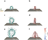 |
Fig. 2. Global evolution of magnetic fields for the SES case (a) t = 5 t0, (c) t = 10 t0 and (e) t = 15 t0 and the FES case at (b) t = 5 t0, (d) t = 15 t0 and (f) t = 40 t0. An animation showing the evolution is available online. |
Then, we used a more comprehensive analysis to explain the differences between the two eruptions in Fig. 3, especially the evolution of the rotation angles. The kinematics of the two MFRs is shown in Fig. 3. The height and rotation angle of MFRs are approximately measured with the flux-rope axis. The axis at each time was traced from the center of the flux-rope positive footpoint. We used the apex height of the flux-rope axis to represent the height of the MFR, and the angle between the direction of the horizontal magnetic field at the axis apex and the negative y-axis were used to represent its rotation angle. Due to the centrosymmetric initial setting of the simulation, the subsequent evolution of the two cases also maintains this characteristic. Therefore, the approximation in which the field line originates from the positive footpoint center as the flux-rope axis is reasonable until the flux-rope axis is significantly reconnected. Figures 3a and b show the connection changes of the axis in two cases. According to the trend of the evolution, two periods are divided in the simulation. In the first stage, the selected axis has the same configuration as the whole flux rope, which means that it can represent the direction of the flux rope. In the second stage, the selected axis has reconnected with other field lines and cannot be regarded as the flux-rope axis. It should be noted that reconnection always exists in the whole evolution, while it is too moderate to lead to a significant deformation in the first stage. This reconnection is plotted in Fig. 3b, which shows a separation between the negative footpoints of the flux-rope axes at t = 34 t0 and at t = 0 or t = 10 t0, indicating the effect of reconnection during the first stage. The division of these two stages is also represented by the semitransparent shadows in Figs. 3c and d. The blue shadow represents the first stage, which shows that the rotation angle increases rapidly in the early stage until it reaches a plateau, after which it no longer increases. This plateau value is around 27° in SES but 90° in FES. Moreover, the angle evolution does not stop at this value in FES. After a period of fluctuation, it experiences a second rapid growth, increasing from 90° to 130°. In the second stage (shaded red area), the selected axis strongly changed its shape as a result of magnetic reconnection, and therefore, the height and rotation angle of the MFR obtained under this approximation are no longer reliable. The main body of the flux rope does not break up in SES, and its axis can still be determined with the help of the distribution of the magnetic squashing degree Q. However, it is hard to trace the same field line all the time with this method. Therefore, we still used the aforementioned method to trace the axis. Our analysis in Sects. 3.3 and 3.4 is mainly based on the evolution of the height and rotation angle in the first stage.
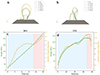 |
Fig. 3. Kinematics evolution of the SES case and FES case. Panels (a) and (b) show several field lines originating from the center of the positive footpoint at (0, 28, 0) Mm in SES and FES. Panels (c) and (d) present the evolution of the flux-rope height (green lines with dots) and rotation angle (yellow lines with crosses) by measuring the height and tangential angle at the apex of the field lines in SES and FES. |
3.2. Magnetic field topology
To quantify the flux-rope topology evolution, we first calculated the distribution of the twist (Tw) value with an approximation in the thin flux tube limit at the bottom. Tw quantifies the degree of entanglement between two infinitely close magnetic field lines, which is defined by
 (4)
(4)
Tw was calculated by the open-source code implemented by Zhang et al. (2022). Then, we used the clearer contour of the Tw distribution to determine the MFR boundary.
After determining the axis and boundary of MFRs, we tracked the topological evolution. For a single MFR, writhe (Wr) and twist (Tg) reflect its geometric properties. Tg is not identical to the aforementioned Tw because the calculation of Tg needs a common axis, and it describes the winding number of an overall structure. For one curve, Wr measures the kink and coil of a closed curve, and it was extended to apply to an open curve (Berger & Prior 2006). Due to the possibility of several extreme values in the height of an open curve, a curve was divided into n parts with monotonic height variation i. For piece i, the local extreme values in the z-direction are [zimin, zimax]. The writhe was split into two parts, the local writhe (Wlocal) and the nonlocal writhe (Wnonlocal). The two formulas are presented as follows:
 (5)
(5)
 (6)
(6)
where Ti is the unit tangent vector on the piece i at a certain z, and z is the unit vector in the z-direction. When the projections of piece i and piece j in the z -direction have the same (opposite) orientation, then σij is +1 (−1). Θij is the angle between the x-axis and the vector from i piece to j piece at the same z-value, where the x-axis is an arbitrary direction perpendicular to z.
For two curves, one of which is defined as the axis, Tg can measure how much the other curve twists about the axis. This is given by
 (7)
(7)
where T(s) is the unit vector along the direction of the magnetic field at a point on the axis, and s represents the length of the magnetic field line between this point and the reference point. V(s) is another unit vector perpendicular to T(s) that points to the other field line. To quantify the geometric properties of the MFR during the eruption, we selected 200 random points inside the Tw contour near the initial positive footpoint of the MFR at each snapshot. Then, the MFR field lines were traced from these points. Because the footpoints shift during the eruption, the flux-rope field lines at different times are not always the same. Finally, Wr and Tg can be calculated with the flux-rope axis and these field lines. The evolutions of Wr and Tg of the two cases are shown in Fig. 4. In SES, Tg first increases and then oscillates in a narrow range, but Wr always increases. In FES, both Tg and Wr exhibit overall monotonic changes over a wider range, and their correlation is more pronounced than in the SES case. Focusing on Tg evolution, we find that the initial Tg0 = 1.42 in SES is slightly higher than that in FES (Tg0 = 1.38). In the subsequent evolution, Tg of the former is always greater than that of the latter.
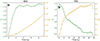 |
Fig. 4. Evolution of the twist and writhe of successful and failed eruptions. Panel (a) shows the evolution of the twist Tg (the green line with dots) and writhe Wr (the yellow line with crosses) in SES. Panel (b) is similar to (a), but for the FES case. |
3.3. Force and torque analysis
Although the topology of an MFR reflects the appearance of its rotation, the origin of the rotation should be traced back to the force acting on the MFR. Figure 5 shows the horizontal Lorentz force distribution of initial MFRs in the two cases. We mainly studied the force along the x-direction (Fx) as the initial MFRs are along the y-direction. A slice at z = 7.5 Mm was chosen to investigate the Fx distribution on the flux-rope legs, which is shown in Figs. 5a and 5b. The two distributions show that Fx in FES is stronger and more widely distributed than in SES. The symmetry of the distributions shows that the force in SES is more inclined to an axial antisymmetry distribution, while in the FES case, the force tends to have a central symmetric distribution.
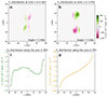 |
Fig. 5. Distribution of the horizontal Lorentz force at t = 0. Panel (a) shows the Fx distribution in horizontal slices z = 7.5 Mm in SES, in which Fx along x+ (x−) is plotted in green (plum). (c) Fx along the axis at t = 0 in SES, where the abscissa represents the y value of the sample point on the axis. Panels (b) and (d) are similar to panels (a) and (c), respectively, but for the FES case. Panels (a) and (b) focus on the center part of the simulation with (−60, 60) Mm in the x range and (−60, 60) Mm in the y range. |
To quantitatively demonstrate the effect of the Lorentz force in inducing the rotation of MFRs in the two simulations, we calculated Fx along the initial flux-rope axes. We traced the axes from the centers of the positive and negative footpoints. The average value of Fx was calculated for two points with the same y-coordinate on the axes. The result is shown in Figs. 5c and 5d, where the distribution of Fx along the axis in two simulations shows a clear central symmetry, but Fx in FES is one order of magnitude larger than that in SES. In particular, the centrosymmetric property of two curves also indicates the clockwise rotation in the following evolution.
Torque is a key element in the rotation of a rigid body around a fixed axis, and the flux-rope rotation we considered here also revolved around the fixed rotation axis of the vertical line above point (0, 0, 0). Although the MFR rotation cannot be completely equivalent to the fixed-axis rotation of a rigid body, the torque analysis can still provide some details. Zhou et al. (2023) have conducted a similar analysis. Unlike their work, we present the distribution of the torque along the flux-rope axis at different times, which provides the impact of the torque on the flux rope morphology. The torque of each point on the flux-rope axis relative to the rotation axis was calculated. Figure A.1 shows the connectivity of the flux rope axis and the spatial distributions of the torque along it at several typical moments. The torque exhibited here is in the z-direction, which reflects the trend of the MFR to rotate clockwise (negative torque) or counterclockwise (positive torque). The purple part represents the negative torque, reflecting the clockwise rotation. At the onset of the simulations (t = 0), nearly the whole axis was dominated by the negative torque, thereby inducing the clockwise rotation. In the early evolution period (t = 5 t0), the range of negative torque then rapidly narrows and only concentrates on the flux-rope legs. The negative torque continually decreases and can be neglected after t = 6 t0 in SES and t = 14 t0 in FES. In addition to the measurement errors that stem from the method, which regards the rotation angle of the axis as the angle of the entire flux rope, a gradual increase in the rotation angle in FES is visible in Fig. 3d. This is more likely attributable to the inertia of the rotating flux rope. As the system evolves further (t = 10 t0 in SES and t = 20 t0 in FES), although the MFR still rotates clockwise, there is almost no negative torque effect, and a strong positive torque even appears in FES, which suggests that the torque is not the main influence on the rotation after these times.
3.4. Magnetic reconnection
In addition to the effects of the Lorentz force and torque, magnetic reconnection also has a significant impact on the morphology of eruptive MFRs. Although we did not set an additional anomalous resistivity in the simulation, the numerical resistivity introduced by the discrete grids and numerical schemes can lead to numerical magnetic reconnection. As mentioned before, the evolution was divided into two stages, and we focused on the influence of reconnection on the flux-rope rotation or on its morphology in the first stage.
We display the footpoints of the flux-rope axes in two simulations (Figs. 6a and 6b), where the field lines of the axes are traced at each time. All the field lines are traced from the position at (0, 28, 0) Mm, and the other end on the bottom plane is marked in rainbow colors representing different times. Figs. 6a and 6b represent the footpoint movement in SES and FES, respectively, from which it is evident that the movement can be divided into three processes: stable at early times, drifting in the medium term, and leaping at late times. In SES, these three processes span over t = 0 ∼ 10 t0, t = 11 t0 ∼ 12 t0, and t > 12 t0, and in FES, they are t = 0 ∼ 23 t0, t = 24 t0 ∼ 34 t0, and t > 34 t0. This further proves the rationality of dividing the simulation into two stages, where early and medium times belong to the first stage and late times belong to the second stage. In accordance with Figs. 3a and 3b, we highlight the footpoint positions during the transition from mid to late times in Figs. 6a and 6b with white circles, which are t = 11 t0 in SES and t = 34 t0 in FES. The footpoint begins to jump in a small area within the active region shortly before t = 34 t0 in FES (Fig. 6b). As this jump does not change the whole trend of the axis movement, we still set t = 34 t0 as the end time of the first stage in FES, after which the overall shape of the selected axis is lost, and the footpoint jumps from the active region to the position of the large-scale background field.
 |
Fig. 6. Footpoint drift in the SES case and FES case. Panel (a) presents the negative footpoints of the axis in SES, where the white circle locates the footpoint position at t = 11 t0. Panel (b) is similar to (a), but in FES, and the white circle locates the footpoint position at t = 34 t0. In both panels, rainbow colors represent different simulation times. Panel (c) shows the axis morphology evolution from t = 24 t0 to t = 32 t0 in FES, and the purple contour shows the QSL at the bottom at t = 24 t0. |
To demonstrate the influence of magnetic reconnection on the magnetic field configuration more vividly, we superposed the field lines at different times in a 3D coordinate system to present the evolution. In Fig. 6c we plot the deformation of the axis originating from (0, 28, 0) Mm during the medium term in FES. The axis slowly slips toward the inner area of the active region along the straight part of QSLs in this period. After this, Fig. 7 shows the strong distortion of the magnetic reconnection on the original magnetic field axis. Referring to the classification of magnetic reconnection in Aulanier & Dudík (2019), the reconnection here is ar − rf reconnection in both cases, where the flux-rope field lines reconnect with external magnetic arcades and generate new flux-rope field lines and flare-loop field lines. In SES, this deformation only involves the leg of the magnetic field line, leading to an increased twist in the flux-rope legs. In FES, this deformation destroys the flux-rope configuration, so that in the second stage of the eruption, the MFR is completely eroded by the external field, leading to the failed eruption.
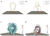 |
Fig. 7. Magnetic field configuration changed by magnetic reconnection. In panels (a) and (b), field lines at two adjacent simulation times are selected to show the axis deformation caused by magnetic recconection in the second stage. The green (the former axis) and yellow lines represent field lines before the reconnection, while the red (the later axis) and plum lines represent field lines after reconnection. The reconnection location is marked by a red star. The two adjacent times in panel (a) are t = 11 t0 and t = 12 t0 in SES, and in panel (b), they are t = 34 t0 and t = 35 t0 in FES. MFRs at t = 10 t0 with QSL contours in xOy and xOz slices are shown in panel (c) in SES and in panel (d) in FES, where the cyan and red lines represent the original RBSL MFR, and the gray lines in panel (d) show the newly formed MFR in FES. |
There is another interesting finding in FES: A new MFR is formed below the original one. We use magnetic fields at t = 10 t0 to present the configuration. In Fig. 7d, both horizontal and vertical QSL contours possess separated inner structures. The MFR evolves from the one inserted by RBSL method, which is plotted in red in Fig. 7b, and another MFR (in gray) forms when FES passes through the original one. That the closed QSLs warp two MFRs proves the separation in topology, and it is evident that a new magnetic configuration formed below the original MFR. Compared to the configuration in SES at the same time (Fig. 7c), neither QSLs nor field lines manifest a new twisted flux rope. The concentric circle contours above the hyperbolic flux tube in the vertical QSLs in particular negate the possibility of a newly formed MFR. This is another significant discrepancy between the two cases.
4. Discussions
4.1. Effects of external toroidal fields
The impact of the external toroidal field on the behavior of MFRs has been analyzed in previous studies such as Isenberg & Forbes (2007) and Kliem et al. (2012). Isenberg & Forbes (2007) initially underscored that the external toroidal field can exert a lateral Lorentz force upon the MFR legs during its ascent, consequently inducing rotation. Subsequently, Kliem et al. (2012) performed a series of zero-β MHD simulations, delineating the evolution of the rotation angle and height of the MFR under varying initial parameters by adjusting the initial twist of the MFR and the ratio of the toroidal and polodial components of the external field. This analysis further underscored the pivotal role of the external toroidal field, denoted as the shear-field component in the referenced work, in facilitating significant rotational motion. We focused on the comparison of the topology and torsional force evolution in two cases. Based on these analysis, we distilled three primary mechanisms by which external toroidal fields influence the rotation of MFRs.
-
Assisting the relaxation of MFR. The external toroidal field can catalyze the relaxation of an MFR, facilitating the conversion from its twist into writhe. Furthermore, comparative analysis from parameter surveys reveals that the external toroidal field impedes the ascent of the MFR, thereby inducing a more gradual relaxation in height. This decelerated ascent in turn fosters lateral relaxation through morphological alterations.
-
Increasing the lateral Lorentz force acting on MFR. The external toroidal field augments the Lorentz force that is exerted on the initial MFR, and it renders the Lorentz force on the legs of the MFR more asymmetric.
-
Promoting the formation of the lower MFR. The existence of torodial fields can engender the formation of a secondary MFR beneath the primary MFR during the eruption. This lower MFR provides a lower toroidal field to the original MFR, thereby amplifying the aforementioned effects of external toroidal fields. The intricacies of the interaction between double MFRs exhibiting large-angle rotation have been elucidated in our previous work Zhang et al. (2024), wherein we clearly present the possible formation mechanism of the lower MFR via tether-cutting reconnection.
4.2. Rotations contributed by magnetic reconnection
In our FES simulation, the negative footpoint of the selected flux-rope axis drifts during the simulation time t = 24 t0 to t = 34 t0 (Fig. 7), which is similar to the slipping magnetic reconnection defined in Aulanier et al. (2006), which is reflected in many observations and numerical simulations (Li & Zhang 2014; Dudík et al. 2016; Janvier et al. 2013). Slipping reconnection is not a single reconnection mode, but the sum of multiple reconnections that occur in the hyperbolic flux tube between adjacent field lines during a certain period in the eruption. The main characteristic of slipping reconnection is the continuous movement of field lines along QSLs. When the footpoints of the field lines do not cross the QSL region boundary, this reconnection only causes a drift in a small range without changing the overall connectivity of the magnetic field lines. Undoubtedly, slipping magnetic reconnection causes the flux-rope footpoints to slide, which is reflected in the slipping motion of coronal dimming regions in observations. In simulations, many works measured the velocity of the slipping reconnection by tracing the field lines from a fixed point at the bottom boundary at a series time (Janvier et al. 2013). Figure 6c uses the same method to display the slipping reconnection in FES case.
Although the connection between slipping magnetic reconnection and the separation of observed flare ribbons was reported in some studies, only a few studies focused on the significance of this reconnection for the rotation of the filament eruption. Through our simulation, we found that the rotation angle of the MFR further increases during this period (t = 24 t0 to t = 34 t0 in Fig. 3d), indicating that the slipping reconnection not only changes the angle of the footpoint connection, but also the upper part of magnetic field lines, which is reflected in the change in the overall rotation angle of the MFR.
In FES, we simply estimated the contribution of the slipping magnetic reconnection to the simulated flux-rope rotation angle. This angle approximately equals the angle between the directions before and after the slipping reconnection of the connection of flux-rope footpoints, and both of them are 30 degrees. This angle change is caused by the movement of the flux-rope footpoint in Fig. 6c, where the flux-rope footpoint slips from one negative flux concentration to the next. The similarity of these two angles inspired us to try to quantify the contribution of the slipping reconnection to the filament rotation by measuring the change angle caused by the movement of the coronal dimming, especially for incidents with ambiguous filament outlines, but clear dimming regions.
We note that the slipping magnetic reconnection takes an unusual form in SES. As a result of the rapid evolution of the MFR in SES, the footpoint drift caused by the slipping reconnection appears as a jump in SES during the time interval of the data storage (see the positions of the footpoints at t = 11 t0 and t = 12 t0 in Fig. 7). As the shape of the axis deforms earlier, we did not quantify the effect of the slipping magnetic reconnection on the rotation angle in SES. However, we inferred that the slipping reconnection contributes to the rotation angle even in the SES case. As described in previous works (e.g., Janvier et al. 2013), the influence of the slipping magnetic reconnection depends on the QSLs around the flux rope. With a similar initial magnetic configuration, the QSLs in SES also move from one flux concentration to the next with the same polarity, which manifests the footpoint movement at the bottom, and this finally contributes to the rotation of the upper flux rope. Moreover, considering the reconnection in Fig. 7a, the magnetic tension force caused by the deformation of the axis at t = 12 t0 pulls the whole flux rope to the negative pole of the external poloidal field. This also confirms the validity of the slipping reconnection in SES.
4.3. Deducing the twist degree of flux ropes from the rotation angle they exhibit in the eruption process
Twist is a significant topology parameter for flux ropes. It determines the initiation and dynamics of the CME flux ropes. On the one hand, the kink instability serves as a basic trigger for solar eruptions. In this scenario, solar eruptions take place when the twist number of their core fields exceeds a specific threshold. On the other hand, due to the helicity conservation, a transfer from the twist number to the writhe number may occur in the eruption process, leading to the rotation in observations. This means that the rotation angles of flux ropes are connected with their twist numbers. According to this, one natural idea is to assess the twist number of the flux ropes from the rotation angle they exhibit in the eruption process.
First, the parametric survey in Kliem et al. (2012) inspired this natural idea. In their case, the highest twist does not always relate to the strongest rotation because the conditions of external toroidal fields differ. In our cases, the existence of the external toroidal field causes the magnetic field lines of the MFR to cross a longer axial distance when they are wound around the flux-rope axis, which to some extent reduces the initial twist of the MFR. Fig. 4 shows that the initial twist (Tg0) of the MFR in FES (Tg0 = 1.38) is slightly weaker than that in SES (Tg0 = 1.42), and from the subsequent analysis, the MFR in FES has a significantly larger rotation angle than that in SES. The following topology evolution in Fig. 4 shows that MFR in FES converts more twist to its writhe than that in SES. In summary, the initial twist of the MFR is not related to the final rotation angle of the MFR. The initial twist of the MFR determines whether it can be triggered under a kink instability, but not the subsequent evolution. Whether the MFR can relax during the eruption process, in other words, whether it can smoothly convert its twist into the flux-rope axis writhe, is an important factor determining the size of the rotation angle. The external toroidal field by promoting this relaxation, helps MFRs achieve large-angle rotation. Regarding these events, it is not suitable to deduce the twist degree of flux ropes with the rotation angle they exhibit in the eruption process.
5. Conclusions
We conducted two simulations of the flux-rope eruption, in which one MFR evolved with the external toroidal field (FES), but the other MFR evolved without it (SES). The discrepancy in the initial setting significantly influenced both the flux-rope configuration and the evolution outcome. Specifically, the FES MFR exhibited a confined eruption with large-angle rotation, whereas the SES MFR successfully erupted with minimal rotation. By comparing the evolution of the physical quantities during the two simulations, we concluded that the external toroidal field promotes the large-angle rotation of the flux-rope system.
First, the external toroidal field facilitated the MFR relaxation, aiding the conversion from its twist to writhe. Second, the MFR evolving under the external toroidal field experiences a stronger lateral Lorentz force, which promotes the rotation. Third, only under the influence of the external toroidal field can a new MFR form below the original one and play a role in the lower toroidal field to further promote the rotation.
Additionally, our simulations revealed another intriguing phenomenon. We find that the slipping magnetic reconnection also contributes to the rotation of the MFR. This reconnection is a joint result of multiple reconnection. It can alter the direction of the line connecting flux-rope footpoints as well as the direction of the MFR apex, which is a potential mechanism to promote the rotation. The further quantitative contributions to the rotation angle caused by different mechanisms need future analysis.
Data availability
Movies associated to Figs. 2 and A.1 are available at https://www.aanda.org
Acknowledgments
X.M.Z. acknowledges Rony Keppens for valuable discussions. X.M.Z., J.H.G., Y.G., and M.D.D. were supported by the National Key R&D Program of China (2022YFF0503004, 2021YFA1600504, and 2020YFC2201201) and NSFC (12333009). The numerical computation was conducted in the High Performance Computing Center (HPCC) at Nanjing University.
References
- Aulanier, G., & Dudík, J. 2019, A&A, 621, A72 [NASA ADS] [CrossRef] [EDP Sciences] [Google Scholar]
- Aulanier, G., Pariat, E., Démoulin, P., & Devore, C. R. 2006, Sol. Phys., 238, 347 [NASA ADS] [CrossRef] [Google Scholar]
- Berger, M. A., & Prior, C. 2006, Journal of Physics A Mathematical General, 39, 8321 [NASA ADS] [CrossRef] [Google Scholar]
- Carmichael, H. 1964, NASA Special Publication, 50, 451 [NASA ADS] [Google Scholar]
- Chen, P. F. 2011, Living Reviews in Solar Physics, 8, 1 [NASA ADS] [CrossRef] [Google Scholar]
- Chen, P. F., Fang, C., Tang, Y. H., & Ding, M. D. 1999, ApJ, 513, 516 [NASA ADS] [CrossRef] [Google Scholar]
- Dudík, J., Polito, V., Janvier, M., et al. 2016, ApJ, 823, 41 [Google Scholar]
- Fan, Y., & Gibson, S. E. 2004, ApJ, 609, 1123 [NASA ADS] [CrossRef] [Google Scholar]
- Guo, J. H., Qiu, Y., Ni, Y. W., et al. 2023, ApJ, 956, 119 [NASA ADS] [CrossRef] [Google Scholar]
- Guo, J. H., Ni, Y. W., Guo, Y., et al. 2024, ApJ, 961, 140 [NASA ADS] [CrossRef] [Google Scholar]
- Hirayama, T. 1974, Sol. Phys., 34, 323 [Google Scholar]
- Isenberg, P. A., & Forbes, T. G. 2007, ApJ, 670, 1453 [NASA ADS] [CrossRef] [Google Scholar]
- Janvier, M., Aulanier, G., Pariat, E., & Démoulin, P. 2013, A&A, 555, A77 [NASA ADS] [CrossRef] [EDP Sciences] [Google Scholar]
- Janvier, M., Aulanier, G., Bommier, V., et al. 2014, ApJ, 788, 60 [Google Scholar]
- Jiang, C., Chen, J., Duan, A., et al. 2021, Frontiers in Physics, 9, 575 [NASA ADS] [Google Scholar]
- Jiang, C., Duan, A., Zou, P., et al. 2023, MNRAS, 525, 5857 [NASA ADS] [CrossRef] [Google Scholar]
- Kay, C., Gopalswamy, N., Xie, H., & Yashiro, S. 2017, Sol. Phys., 292, 78 [NASA ADS] [CrossRef] [Google Scholar]
- Keppens, R., Popescu Braileanu, B., Zhou, Y., et al. 2023, A&A, 673, A66 [NASA ADS] [CrossRef] [EDP Sciences] [Google Scholar]
- Kliem, B., & Török, T. 2006, Phys. Rev. Lett., 96, 255002 [Google Scholar]
- Kliem, B., Török, T., & Thompson, W. T. 2012, Sol. Phys., 281, 137 [NASA ADS] [Google Scholar]
- Kopp, R. A., & Pneuman, G. W. 1976, Sol. Phys., 50, 85 [Google Scholar]
- Li, T., & Zhang, J. 2014, ApJ, 791, L13 [NASA ADS] [CrossRef] [Google Scholar]
- Lynch, B. J., Antiochos, S. K., Li, Y., Luhmann, J. G., & DeVore, C. R. 2009, ApJ, 697, 1918 [NASA ADS] [CrossRef] [Google Scholar]
- Manchester, W., Kilpua, E. K. J., Liu, Y. D., et al. 2017, Space Sci. Rev., 212, 1159 [Google Scholar]
- Myers, C. E., Yamada, M., Ji, H., et al. 2015, Nature, 528, 526 [Google Scholar]
- Srivastava, N., & Venkatakrishnan, P. 2004, Journal of Geophysical Research (Space Physics), 109, A10103 [NASA ADS] [Google Scholar]
- Sturrock, P. A. 1966, Nature, 211, 695 [Google Scholar]
- Titov, V. S., Török, T., Mikic, Z., & Linker, J. A. 2014, ApJ, 790, 163 [NASA ADS] [CrossRef] [Google Scholar]
- Titov, V. S., Downs, C., Mikić, Z., et al. 2018, ApJ, 852, L21 [NASA ADS] [CrossRef] [Google Scholar]
- Török, T., & Kliem, B. 2005, ApJ, 630, L97 [Google Scholar]
- Török, T., Kliem, B., & Titov, V. S. 2004, A&A, 413, L27 [NASA ADS] [CrossRef] [EDP Sciences] [Google Scholar]
- Tsurutani, B. T., Gonzalez, W. D., Tang, F., Akasofu, S. I., & Smith, E. J. 1988, J. Geophys. Res., 93, 8519 [NASA ADS] [CrossRef] [Google Scholar]
- Vourlidas, A., Colaninno, R., Nieves-Chinchilla, T., & Stenborg, G. 2011, ApJ, 733, L23 [NASA ADS] [CrossRef] [Google Scholar]
- Wang, C., Chen, F., Ding, M., & Lu, Z. 2023, ApJ, 956, 106 [NASA ADS] [CrossRef] [Google Scholar]
- Wheatland, M. S., Sturrock, P. A., & Roumeliotis, G. 2000, ApJ, 540, 1150 [Google Scholar]
- Williams, D. R., Török, T., Démoulin, P., van Driel-Gesztelyi, L., & Kliem, B. 2005, ApJ, 628, L163 [NASA ADS] [CrossRef] [Google Scholar]
- Wilson, R. M. 1987, Planet. Space Sci., 35, 329 [NASA ADS] [CrossRef] [Google Scholar]
- Xia, C., Teunissen, J., El Mellah, I., Chané, E., & Keppens, R. 2018, ApJS, 234, 30 [Google Scholar]
- Yurchyshyn, V., Abramenko, V., & Tripathi, D. 2009, ApJ, 705, 426 [NASA ADS] [CrossRef] [Google Scholar]
- Zhang, P., Chen, J., Liu, R., & Wang, C. 2022, ApJ, 937, 26 [NASA ADS] [CrossRef] [Google Scholar]
- Zhang, X. M., Guo, J. H., Guo, Y., Ding, M. D., & Keppens, R. 2024, ApJ, 961, 145 [NASA ADS] [CrossRef] [Google Scholar]
- Zhou, Z., Cheng, X., Zhang, J., et al. 2019, ApJ, 877, L28 [NASA ADS] [CrossRef] [Google Scholar]
- Zhou, Z., Jiang, C., Yu, X., et al. 2023, Frontiers in Physics, 11, 1119637 [NASA ADS] [CrossRef] [Google Scholar]
Appendix A: Torque distribution along the axis
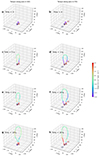 |
Fig. A.1. Torque distribution along the axis at (a) t = 0, (c) t = 5 t0, (e) t = 6 t0, and (g) t = 10 t0 in SES, and (b) t = 0, (d) t = 5 t0, (f) t = 14 t0, and (h) t = 20 t0 in FES, where the positive (negative) torque promotes the counterclockwise (clockwise) rotation is shown in red (purple). In all panels, the magnetic contours of +20 Gauss (dark red) and -20 Gauss (dark blue) are superimposed on the bottom plane. The white lines show polarity inversion lines in each panel. An animation showing the above evolutions is available online. |
All Tables
Parameters of external field charges and flux ropes in the initial setups of the two simulations.
All Figures
|
Fig. 1. Initial magnetic field configurations. (a, c) MFR and external field lines of SES in top and side views, (b, d) and those of FES in the same views. |
| In the text | |
|
Fig. 2. Global evolution of magnetic fields for the SES case (a) t = 5 t0, (c) t = 10 t0 and (e) t = 15 t0 and the FES case at (b) t = 5 t0, (d) t = 15 t0 and (f) t = 40 t0. An animation showing the evolution is available online. |
| In the text | |
|
Fig. 3. Kinematics evolution of the SES case and FES case. Panels (a) and (b) show several field lines originating from the center of the positive footpoint at (0, 28, 0) Mm in SES and FES. Panels (c) and (d) present the evolution of the flux-rope height (green lines with dots) and rotation angle (yellow lines with crosses) by measuring the height and tangential angle at the apex of the field lines in SES and FES. |
| In the text | |
|
Fig. 4. Evolution of the twist and writhe of successful and failed eruptions. Panel (a) shows the evolution of the twist Tg (the green line with dots) and writhe Wr (the yellow line with crosses) in SES. Panel (b) is similar to (a), but for the FES case. |
| In the text | |
|
Fig. 5. Distribution of the horizontal Lorentz force at t = 0. Panel (a) shows the Fx distribution in horizontal slices z = 7.5 Mm in SES, in which Fx along x+ (x−) is plotted in green (plum). (c) Fx along the axis at t = 0 in SES, where the abscissa represents the y value of the sample point on the axis. Panels (b) and (d) are similar to panels (a) and (c), respectively, but for the FES case. Panels (a) and (b) focus on the center part of the simulation with (−60, 60) Mm in the x range and (−60, 60) Mm in the y range. |
| In the text | |
|
Fig. 6. Footpoint drift in the SES case and FES case. Panel (a) presents the negative footpoints of the axis in SES, where the white circle locates the footpoint position at t = 11 t0. Panel (b) is similar to (a), but in FES, and the white circle locates the footpoint position at t = 34 t0. In both panels, rainbow colors represent different simulation times. Panel (c) shows the axis morphology evolution from t = 24 t0 to t = 32 t0 in FES, and the purple contour shows the QSL at the bottom at t = 24 t0. |
| In the text | |
|
Fig. 7. Magnetic field configuration changed by magnetic reconnection. In panels (a) and (b), field lines at two adjacent simulation times are selected to show the axis deformation caused by magnetic recconection in the second stage. The green (the former axis) and yellow lines represent field lines before the reconnection, while the red (the later axis) and plum lines represent field lines after reconnection. The reconnection location is marked by a red star. The two adjacent times in panel (a) are t = 11 t0 and t = 12 t0 in SES, and in panel (b), they are t = 34 t0 and t = 35 t0 in FES. MFRs at t = 10 t0 with QSL contours in xOy and xOz slices are shown in panel (c) in SES and in panel (d) in FES, where the cyan and red lines represent the original RBSL MFR, and the gray lines in panel (d) show the newly formed MFR in FES. |
| In the text | |
|
Fig. A.1. Torque distribution along the axis at (a) t = 0, (c) t = 5 t0, (e) t = 6 t0, and (g) t = 10 t0 in SES, and (b) t = 0, (d) t = 5 t0, (f) t = 14 t0, and (h) t = 20 t0 in FES, where the positive (negative) torque promotes the counterclockwise (clockwise) rotation is shown in red (purple). In all panels, the magnetic contours of +20 Gauss (dark red) and -20 Gauss (dark blue) are superimposed on the bottom plane. The white lines show polarity inversion lines in each panel. An animation showing the above evolutions is available online. |
| In the text | |
Current usage metrics show cumulative count of Article Views (full-text article views including HTML views, PDF and ePub downloads, according to the available data) and Abstracts Views on Vision4Press platform.
Data correspond to usage on the plateform after 2015. The current usage metrics is available 48-96 hours after online publication and is updated daily on week days.
Initial download of the metrics may take a while.