| Issue |
A&A
Volume 688, August 2024
|
|
|---|---|---|
| Article Number | A96 | |
| Number of page(s) | 22 | |
| Section | Extragalactic astronomy | |
| DOI | https://doi.org/10.1051/0004-6361/202449212 | |
| Published online | 09 August 2024 | |
Radiative and mechanical energies in galaxies
I. Contributions of molecular shocks and PDRs in 3C 326 N
1
Laboratoire de Physique de l’École Normale Supérieure, ENS, Université PSL, CNRS, Sorbonne Université, Université Paris Cité, 75005 Paris, France
e-mail: This email address is being protected from spambots. You need JavaScript enabled to view it.
2
Observatoire de Paris, PSL University, Sorbonne Université, LERMA, 75014 Paris, France
3
Sorbonne Université, CNRS, UMR 7095, Institut d’ Astrophysique de Paris, 98bis bd Arago, 75014 Paris, France
4
Université Paris-Saclay, CNRS, Institut d’Astrophysique Spatiale, 91405 Orsay, France
Received:
11
January
2024
Accepted:
2
May
2024
Abstract
Context. Atomic and molecular lines emitted from galaxies are fundamental tracers of the medium responsible for the emission and contain valuable information regarding the energy budget and the strength of the different feedback mechanisms.
Aims. The goal of this work is to provide a new framework for the interpretation of atomic and molecular lines originating from extragalactic sources and a robust method to deduce the mechanical and radiative energy budget from a set of observations.
Methods. Atomic and molecular lines detected in a given object are assumed to result from the combination of distributions of shocks and photo-dissociation regions (PDRs) within the observational beam. The emission of individual structures is computed using the Paris-Durham shock code and the Meudon PDR code over a wide range of parameters. The total emission is then calculated assuming probability distribution functions for shocks and PDRs. A distance between the observational dataset and the model is finally defined based on the ratios of the observed to the predicted intensities.
Results. As a test case scenario, we consider the radio galaxy 3C 326 N. The dataset is composed of 12 rotational and ro-vibrational lines of H2 and the fine structure lines of C+ and O. Our interpretative framework shows that both shocks and PDRs are required to explain the line fluxes. Surprisingly, viable solutions are obtained at low density only (nH < 100 cm−3), indicating that most of the emission originates from diffuse interstellar matter. The optimal solution, obtained for nH = 10 cm−3, corresponds to a distribution of low-velocity shocks (between 5 and 20 km s−1) propagating in PDR environments illuminated by a UV radiation field ten times larger than that in the solar neighborhood. This solution implies that at least 4% of the total mass carried by the PDRs is shocked. The H2 0-0 S(0) 28 μm, [CII] 158 μm, and [OI] 63 μm lines originate from the PDR components, while all the other H2 lines are mostly emitted by shocks. The total solid angles sustained by PDRs and shocks imply that the radiative and mechanical energies reprocessed by these structures are LUV = 6.3 × 10⁹ L⊙ and LK = 3.9 × 10⁸ L⊙, respectively, in remarkable agreement with the values of the IR luminosity deduced from the fit of the spectral energy distribution (SED) of 3C 326 N, and consistent with a small fraction of the active galactic nuclei (AGN) jet kinetic power dissipated in the interstellar medium (≈1%).
Conclusions. This work shows that the radiative and mechanical energy budget of galaxies can be derived from the sole observations of atomic and molecular lines. It reveals the unexpected importance of the diffuse medium for 3C 326 N, in contrast to previous studies. A last-minute comparison of the model to new JWST data obtained in 3C 326 N shows a striking agreement and demonstrates the ability of the model to make accurate predictions. This framework opens new prospects for the prediction and interpretation of extragalactic observations, in particular in the context of JWST observations.
Key words: shock waves / ISM: kinematics and dynamics / ISM: molecules / photon-dominated region (PDR) / galaxies: ISM / galaxies: jets
© The Authors 2024
 Open Access article, published by EDP Sciences, under the terms of the Creative Commons Attribution License (https://creativecommons.org/licenses/by/4.0), which permits unrestricted use, distribution, and reproduction in any medium, provided the original work is properly cited.
This article is published in open access under the Subscribe to Open model. This email address is being protected from spambots. You need JavaScript enabled to view it. to support open access publication.
1. Introduction
Galaxies are dynamic systems where diverse energy sources and sinks shape their evolution over cosmic time. The intricate interplay between dynamics, energy dissipation, and star formation constitutes the essence of galaxy formation and evolution (e.g., Pfenniger 2010). For instance, in the hypothetical absence of radiative losses, the kinetic energy released by gravitational accretion onto halos would keep the gas unbound and galaxies would not form at all (Benson 2010). It is therefore of paramount importance to understand and quantify how and where radiative and mechanical energies are reprocessed and dissipated in the multiphase gas of galaxies.
The reprocessing of radiative and mechanical energy in the interstellar medium (ISM) regulates the distribution of gas phases (e.g., Vazquez-Semadeni 2009), the formation of molecular clouds and stars (Klessen & Hennebelle 2010), and the feedback mechanisms (Cielo et al. 2018; Ostriker & Kim 2022). Mechanical processes encompass the momentum input from stellar winds (Krumholz et al. 2014), supernovae (Fierlinger et al. 2016), and active galactic nuclei (AGN) (Ciotti et al. 2010). Simultaneously, radiative processes involve cooling through thermal and nonthermal emissions across the electromagnetic spectrum, from radio waves to gamma rays. The dissipation of radiative and mechanical energy in the ISM is intricately linked to the gas heating and cooling mechanisms, governed by the microphysics. The thermodynamic and chemical states of the gas significantly influence ISM observables, including ionic, atomic, and molecular line emissions. Those gas properties depend on factors such as density, metal and dust abundance, and the strengths of heating and/or ionization sources such as the ultraviolet (UV) radiation field and cosmic rays.
Efforts to model line and continuum emission in galaxies provide a means to constrain dominant gas excitation mechanisms and to quantify the reprocessed energy required to reproduce observations. Nonetheless, the complexity of the ISM poses significant challenges in solving radiative transfer within galaxies (Kim et al. 2022). As a result, thermal equilibrium and energy balance arguments are frequently employed to simplify calculations. For instance, contemporary codes used to replicate the panchromatic spectral energy distributions (SEDs) of galaxies often assume that stellar UV and near-infrared (NIR) light is absorbed by interstellar dust and subsequently re-emitted in the far-infrared (FIR) domain (da Cunha et al. 2008; Carnall et al. 2018; Boquien et al. 2019), primarily in photo-dissociation regions (PDRs) situated at the interfaces between molecular clouds and diffuse regions of atomic and ionized gas. This assumption is commonly employed to constrain the amount of reprocessed radiative energy from FIR observations and deduce the properties of infrared (IR) galaxies (e.g., Casey et al. 2014).
The physical modeling of spectral line cooling from galaxies, arising from the de-excitation of ions, atoms, and molecules, typically focuses on specific chemical states of the gas (ionized, atomic, or molecular), ISM phases (particular temperature or density ranges), or energy types (electromagnetic radiation, cosmic rays, or mechanical dissipation). For instance, well-established photo-dissociation codes like CLOUDY (Ferland et al. 2017) or the Meudon PDR code (Le Petit et al. 2006) are commonly employed to model the reprocessing of radiative energy, thereby constraining excitation mechanisms and physical conditions of X-ray or UV-irradiated gas in galaxies (e.g., Polles et al. 2021). Conversely, the reprocessing of mechanical energy in ionized, atomic, or molecular media has been incorporated into codes such as MAPPINGS (Allen et al. 2008) or the Paris-Durham shock code (Flower 2003; Godard 2019). The majority of investigations employing the aforementioned models to characterize molecular line emissions from galaxies conclude that both radiative and mechanical processes contribute substantively to the observed gas excitation. As an illustration, the spectral line energy distribution (SLED) of the carbon monoxide (CO) molecule is frequently modeled through a mix of PDRs, X-ray dominated regions (XDRs), and shocks (Meijerink et al. 2013; Mingozzi et al. 2018; Esposito et al. 2022).
This paper addresses the reprocessing of energy in the molecular phase of the ISM. We present a method to estimate the relative contributions of shocks and PDRs to the observed line emission from galaxies, with a focus on H2 lines. Given that H2 can form on interstellar dust at elevated temperatures (≈50 to 250 K, Grieco et al. 2023) and that the H2 rotational levels are separated by a few hundred Kelvin, it emerges as a significant coolant for warm gas and, consequently, a key participant in the reprocessing of radiation within PDRs (Habart et al. 2005; Shaw et al. 2009) and the dissipation of kinetic energy within molecular shocks (Flower 1999; Kristensen et al. 2023). A previous study by Lesaffre (2013) used probability distribution functions of shock velocities to model the rotational and ro-vibrational lines of H2 in molecular gas heated by shock waves. These emission lines serve as indicators of mechanical energy dissipation (Lesaffre et al. 2020), particularly within galaxies where the total power of IR H2 line emissions exceeds what can be accounted for by the exclusive reprocessing of the available UV radiative luminosity (Guillard & Boulanger 2009; Ogle et al. 2010; Nesvadba et al. 2010; Herrera et al. 2012; Guillard et al. 2015a,b).
This paper presents an extension of the framework presented in Lehmann & Godard (2022), where we now combine distributions of shocks and PDR models. The state-of-the-art codes used to model the line emission are presented in Sect. 2. The toy model we use to describe the line fluxes from an ensemble of shocks and PDRs is described in Sect. 3, as is the methodology used to fit a suite of emission lines with grids of models. In Sect. 4 we apply this modeling to the 3C 326 N radio-galaxy, constraining UV- and shock-processed gas mass and energy budgets. In Sect. 5 and conclude in Sect. 6, we provide predictions of the suite of ro-vibrational H2 emission lines that will be observed with the JWST. Throughout this work, we assume a modern flat cosmology (Planck Collaboration VI 2020) with Ωm = 0.315, ΩΛ = 0.685, Ωb = 0.0493, and H0 = 67.4 km s−1 Mpc−1.
2. Shock and PDR models
For this paper, two publicly available codes were used to model PDR and shock emissions: the Meudon PDR code1 (Le Petit et al. 2006) and the Paris-Durham shock code2 (Flower 2003; Godard 2019).
2.1. Grids of PDR models
The Meudon PDR code is a model designed to study the thermal and chemical structures of photo-dissociation regions with a constant proton density, nH, or a constant thermal pressure. The geometry, the main assumptions, and the physical ingredients included in the code are described in Le Petit et al. (2006). In a nutshell, the model considers a 1D plane-parallel and static slab of gas and dust illuminated on both sides by semi-isotropic radiation fields, each of which is set to the standard interstellar radiation field (ISRF, Mathis et al. 1983) and scaled with a parameter G0. The size of the cloud is set by its total extinction Av max. Within this geometry, the model solves the radiative transfer, taking into account the detailed absorption and emission processes induced by dust and gas compounds, and the thermal and chemical states of matter at equilibrium, through the inclusion of an extensive chemical network.
In addition to the chemical composition of the gas, the model also solves the excitation of atomic and molecular species including the populations of 250 ro-vibrational levels of H2. In particular, the excitation of the fine structure levels of C+ and O is computed including excitation by collisions with H, H2, and electrons (for C+) and with H, H+, H2, He, and electrons (for O). The populations of the ro-vibrational levels of H2 are computed taking into account excitation by collisions with H, He, H2, and H+, the probability of exciting H2 at formation on grain surfaces, and the excitation by radiative pumping of the electronic lines of molecular hydrogen followed by fluorescence. The emerging line fluxes of all these species are finally calculated by integrating the emissivities over the entire slab up to Av max.
The grid of models used in this paper is a subsample of the precomputed models obtained with the 1.5.4 version of the Meudon PDR code and publicly available on the InterStellar Medium DataBase service (ISMDB3). We consider PDR models at constant proton density only, with a left-side illumination scaling factor G0 = 1 or 10 and a right-side illumination scaling factor G0 = 1. The range of parameters explored here is shown in Table 1.
PDR and shock model parameters.
2.2. Grids of shock models
The Paris-Durham shock code is a model designed to study the dynamical, thermal, and chemical evolution of molecular shocks propagating at a velocity vs in a magnetized and irradiated environment with an initial proton density nH and an initial magnetic field strength set by a magnetic parameter b. The geometry, the main assumptions, and the physical ingredients included in the code are described in Godard (2019). In a nutshell, the model considers a 1D plane-parallel shock wave at steady-state traveling in a photo-dissociation region. The shock is assumed to be irradiated upstream by a semi-isotropic radiation field set to the standard interstellar radiation field (ISRF, Mathis et al. 1983) and scaled with a parameter G0, and to be initially located at a position within the PDR set by a visual extinction Av = 1.0 (Kristensen et al. 2023). Within this geometry, the model follows in a Lagrangian frame, the out-of-equilibrium evolution of a fluid particle during its trajectory from the pre-shock medium to the post-shock gas, starting from initial conditions at thermal and chemical equilibrium.
In addition to the chemical composition of the gas, the model solves the excitation of atomic and molecular species and the out-of-equilibrium evolutions of the first 150 ro-vibrational levels of H2. In particular, the excitation of the fine structure levels of C+ and O and of the ro-vibrational levels of H2 are computed taking into account all the processes included in the Meudon PDR code and described in the previous section. The emerging line fluxes of all these species are finally calculated by integrating the emissivities over the entire shock up to the point where 99.9% of the input mechanical energy is dissipated (see Eq. (1) of Kristensen et al. 2023). This cutting point is chosen to prevent the inclusion of large amounts of cold post-shocked gas in the computation of line intensities and to ensure that emerging intensities mostly come from the reprocessing of mechanical energy input and not from other sources of energy (UV and IR fields, cosmic rays).
Although large grids of models obtained with the Paris-Durham shock code have been recently computed by Kristensen et al. (2023) and are publicly available on the ISMDB service, we decided here to adopt a more refined set of shock velocities. The values of the parameters covered by the grid are shown in Table 1. The shock velocity ranges between 1 and 40 km s−1 in steps of 1 km s−1.
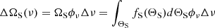
3. Ensembles of shocks and PDRs
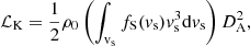
When an extragalactic object is observed, the instrumental beam captures the emission from all the phases of the ISM. As schematized in Fig. 1, these include the hot and diffuse ionized gas, the diffuse and irradiated neutral media, and the dense molecular gas. In principle, all these phases contribute to the reprocessing of the radiative energy input originating from the AGN and the stars, and the mechanical energy input originating, for instance from the interaction between the jet and the galactic disk. Since we focused on molecular lines and on typical tracers of the neutral interstellar medium, we neglected the contribution of the hot ionized phase. Under this approximation, we developed a simplified model in which the reprocessing of the input UV radiative energy occurs in idealized 1D PDRs, and the reprocessing of the input mechanical energy occurs in idealized 1D shock structures.
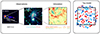 |
Fig. 1. Schematic representation of the multiphase ISM in a galaxy. Left: radio emission observed in 3C 326 N with the Westerbork Synthesis Radio Telescope (WSRT) 21 cm (Willis & Strom 1978) and Spitzer/IRAC composite image (Ogle et al. 2007) at 3.6, 4.5, and 8.0 μm, showing the 3C 326 N galaxy (and its southern companion). The 3.7″ × 3.7″ (6.4 × 6.4 kpc) square (not-to-scale) represents the solid angle Ωobs over which line emissions are observed. Center: cutout showing the projected proton density from a numerical simulation of the interaction between a radio jet and the central part of a multiphase galactic disk (from Murthy et al. 2022). The different colors show the parsec-scale multiphase structure, with the dense irradiated medium in red (nH ≥ 103 cm−3), the shock diffuse gas in yellow (i.e., nH ∼ 10 − 103 cm−3), and the hot X-ray plasma in green (nH ∼ 1 cm−3). Right: simplified model used in this paper where the observational beam is supposed to encompass distributions of shock and PDR surfaces (see Fig. A.1). |
3.1. Toy model
As described in Appendix A, we consider that an ensemble of shock and PDR surfaces, subtending total solid angles ΩS and ΩP, are captured within an observational beam of solid angle Ωobs (see Fig. 1). The cumulative fluxes originating from shock and PDR structures collectively contribute to the observed emission lines. For simplicity, the total solid angles ΩS and ΩP are assumed to follow 1D probability distribution functions denoted by fS and fP. The shock distribution is supposed to depend on the shock velocity vs and the PDR distribution is supposed to depend on the illumination factor G0, yielding the specific functional forms fS(vs) = dΩS/dvs and fP(G0) = dΩP/dG0, respectively.
Considering that the continuum absorption due to the shock and PDR surfaces is negligible and that no cross-absorption occurs between the surfaces4 (see Eqs. (A.8) and (A.9)), we derive a simple expression of the continuum subtracted line flux (see Eq. (A.11)). It follows that the integrated intensity of each line (in erg s−1 cm−2 sr−1) is given by
 (1)
(1)
where IS(vs) and IP(G0) are the line integrated intensities emitted by one shock of velocity vs and one PDR of illumination factor G0, respectively. The superscript “m” stands for model.
It should be noted that the framework can be easily extended to other types of contributions to the line emission, for instance the XDR and HII region. In such cases, the right-hand side of Eq. (1) can be partitioned into multiple components.
3.2. Comparison between model and observations: Distance minimization
This toy model can be used to interpret an ensemble of integrated intensities of unresolved emission lines. The confrontation of the model to the observations only requires defining a distance between the modeled and the observed intensities. Minimizing this distance leads to the characterization of the distributions of shocks and PDRs within the beam, in particular the number of shocks and PDRs and the distribution of shock velocities required to reproduce the observations.
We consider an ensemble of N emission lines. According to Eq. (1), the modeled intensity of each line j writes
 (2)
(2)
We define the distance between the modeled and the observed intensities of each line j as the difference between the model prediction and the observation in log space
 (3)
(3)
where  is the observed intensity of line j and Wj is the associated 1σ uncertainty. The total quadratic distance between the model and the ensemble of observations is calculated as the sum of the quadratic distances of all emission lines
 (4)
(4)
Equation (4) is nothing more than the distance, in log scale, between the model and a hypercube in N dimensions defined by the observed intensities and their associated uncertainties. This distance also bears a natural physical meaning. For instance, a distance of 1 dex implies that at most one observation is underestimated or overestimated by a factor of 10.
With this definition of the distance, the interpretation of an ensemble of atomic and molecular lines is performed using the following three-step procedure:
First, the 1D distribution functions fS(vs) and fP(G0) are assumed to have known functional forms. Based on the results of numerical studies (e.g., Lehmann et al. 2016), we adopt by default here an exponential distribution of shock velocities: fS(vs) = (ΩS/σvs)exp(−vs/σvs), where σvs is the dispersion of shock velocities. For simplicity, we consider a Dirac delta distribution of the PDR illumination factor: fP(G0) = ΩPδ(G0).
Second, the modeled intensities are computed using Eq. (2) over a wide range of the parameters ΩS, σvs, and ΩP describing the distributions fS and fP, assuming that all the other parameters (e.g., nH, b; see Table 1) are constants. The associated distances d(ΩS, σvs, ΩP) between the model and the set of observations are computed with Eq. (4).
Finally, the global and local minima of the distance are searched for to identify the distributions fS and fP that fall the closest to the observational dataset.
3.3. Mechanical an UV-reprocessed luminosities
The probability distribution functions fS and fP directly provide the amount of mechanical and radiative energies reprocessed by shocks and PDRs. The rate of dissipation of mechanical energy of a steady-state shock propagating at a velocity vs in a medium with pre-shock mass density ρ0 is
 (5)
(5)
where 𝒜 stands for the shock surface area (see Fig. A.1). The total mechanical luminosity dissipated (in erg s−1 sr) by a distribution of shocks at different velocities therefore writes
 (6)
(6)
where DA is the angular diameter distance.
As explained in Sect. 2.1, a PDR is modeled as a plane-parallel cloud illuminated by a semi-isotropic ISRF with a fixed scaling factor on the backside and a varying radiation factor G0 on the front side. The integrated flux of the Mathis et al. (1983) ISRF (in erg cm−2 sr−1) from 912 to 2400 Å (Le Petit et al. 2006) implies that the UV-reprocessed power by one PDR is
 (7)
(7)
The total reprocessed UV-luminosity for an ensemble of PDRs that follow a 1D probability distribution fP(G0), therefore writes
 (8)
(8)
3.4. Shock and PDR masses
The probability distribution functions fS and fP also directly provide the total masses of shocks and PDRs within the observational beam. The total mass of shocked material writes
 (9)
(9)
where mH is the hydrogen mass and NH(vs) is the proton column density across a shock of velocity vs. The total mass of PDR material depends on the typical PDR size or equivalently their typical visual extinction Av. This mass writes
 (10)
(10)
where NH(Av) is the proton column density evaluated at a given visual extinction Av.
4. Application to the radio galaxy 3C 326 N
Active galaxies are natural sources to investigate the importance of mechanical heating (Begelman & Ruszkowski 2005). As a test-case scenario, we therefore apply the framework developed in Sect. 3 to the radio galaxy 3C 326 N. This particular choice is motivated by the unique features of 3C 326 N, which include a notably low star formation rate (SFR) (Ogle et al. 2010, ∼0.07 M⊙ yr−1), a substantial reservoir of molecular content (Nesvadba et al. 2011, ∼2 × 10⁹ M⊙), and the conspicuous presence of H2 emission lines (see Appendix B). The low SFR in this galaxy implies that the gas is weakly irradiated by the stellar UV radiation field, and therefore favors the contributions of shocks in line emission (Guillard et al. 2012, 2015b). As described in Appendix B, we consider a dataset composed of 14 emission lines, including H2 pure-rotational and ro-vibrational transitions, alongside [CII] 158 μm and [OI] 63 μm emission lines. The observed fluxes and uncertainties used for the distance minimization (see Eq. (3)) are listed in Table B.2.
The grids of PDR and shock models are described in Table 1. Any observed emission line is assumed to result from the combination of PDRs and shocks within the observational beam.5 For simplicity, we consider that all PDRs and shocks have a unique and common density and pre-shock density nH, and are illuminated by a unique and common UV radiation field characterized by a scaling factor G0. As explained in Sect. 2, we also consider that shocks propagate in PDRs at a typical visual extinction6Av = 1.0. Finally, we assume that all shocks propagate in a medium with a constant transverse magnetic field strength B0, scaled by the magnetization parameter b that follows the relation B0 = b(nH/cm−3)1/2 μG.
As a fiducial model, we adopt nH = 10 cm−3, b = 0.1, and G0 = 10. The choice of density comes from the exploration of the parameters and the comparison with the observations shown in the following sections. The choice of the illumination factor comes from the measurements of the UV emission (Ogle et al. 2010) and of the spectral SED of dust in the IR (Guillard et al. 2015b), which suggest  and G0 = 9 ± 1, respectively.
In this section we first present the minimization process and the optimal shock and PDR distributions obtained for the fiducial model, and then show how this optimal distribution depends on the fixed parameters. In principle, the effects of all fixed parameters should be discussed. However, we find that both G0 and b have a minor impact on the distribution of shocks and PDRs required to explain the observations as long as 1 ≤ G0 ≤ 10 and b ≤ 1. We therefore limit our discussion to the effect of the gas density only.
4.1. Likelihood analysis of the fiducial model
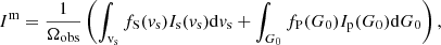
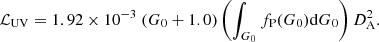
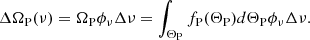
The results of the minimization procedure applied to the fiducial model are displayed in Fig. 2, which shows the distance computed with Eqs. (3) and (4) as a function of the parameters of the shock and PDR distributions, ΩS, σvs, and ΩP. This analysis highlights several key features.
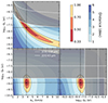 |
Fig. 2. 2D cutoff of the likelihood distributions of the main parameters describing the shock and the PDR distributions obtained for the fiducial model. The parameters are the total shock solid angle ΩS, the dispersion of the shock velocities σvs, and the PDR total solid angle ΩP. The color-coding represents the distance in dex units. The 0.5, 0.7, and 1.0 dex limits are highlighted with dashed black lines. The straight black dashed lines and the black points indicate the position of the global minimum. The gray areas represent the regions where the assumption on the radiative transfer regarding cross-absorption between surfaces breaks down. The criterion is more stringent for the [OI] 63 μm line (gray area above the white solid line) than for the [CII] 158 μm line (gray area above the white dashed line), and is always fulfilled for H2 lines (see Appendix A). |
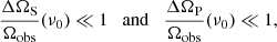
First and foremost, we find that the fiducial model leads to distances as small as 0.33 dex. As we show in Fig. 3, the value of the global minimum implies that the 14 observational constraints, which include atomic and molecular emissions, are all reproduced within a factor smaller than 2, a surprising result given the simplicity of the adopted distributions and the 1D plane-parallel geometry of the models. The global minimum is obtained for distributions of shocks and PDRs with total solid angles ΩS = 1.9 × 10⁻⁸ sr and ΩP = 1.2 × 10⁻⁹ sr, and a shock velocity distribution characterized by σvs ≈ 4 km s−1. This result implies that there are about ten shock surfaces per PDR surface in the observational beam. It also indicates that the number of shocks rapidly decreases with the shock velocity in agreement with the distribution of shock velocities derived in magnetohydrodynamic (MHD) simulations of interstellar turbulence (see Fig. 9 of Lehmann et al. 2016). Interestingly, the optimal value of  implies that the peak of dissipation of mechanical energy occurs for
  and that most of the dissipation is mediated by shocks with velocities between ∼5 and ∼20 km s−1.
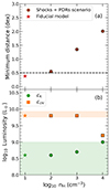 |
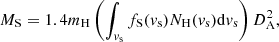
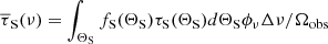
Fig. 3. Solution for a combination of shocks and PDRs, assuming an exponential probability distribution function. Panel (a): distance vs. the medium’s density. The dashed line represents a 0.5 dex limit (i.e., a factor of 3 difference between observed and modeled line intensities) to guide the eye. Panel (b): derived mechanical-reprocessed luminosity from Eq. (6) as well as the UV-reprocessed luminosity from Eq. (8) as a function of density are shown in green and orange, respectively. The green area represents < 1% of the estimated jet kinetic luminosity of 3C 326 N, while the orange area represents the SED estimation of the reprocessed UV-luminosity (see Appendix C). |
Another main feature of this analysis is the uniqueness of the optimal solution. As suggested by Fig. 2, we find that the entire parameter space is characterized by only one global minimum, which occupies a finite volume in the parameter space, and no local minima. This absence of local minima indicates that there are no complex degeneracies between the parameters of the shock and PDR distributions. In particular, the large distances obtained for small values of ΩS or ΩP imply that both shocks and PDRs are required to explain the observational dataset and that no acceptable solution (with a distance smaller than one dex) can be obtained with a sole distribution of shocks or PDRs. Nevertheless, Fig. 2 also reveals some degeneracy between ΩS and σvs: solutions with distances smaller than 0.5 dex can be obtained for ΩS varying over one order of magnitude and σvs over a factor of 2. This degeneracy comes from the fact that the emission lines of H2 mostly originate from shocks with a specific range of velocities (see Sect. 5) whose numbers are set by both ΩS and σvs.
Figure 2 finally reveals the domain of validity of the radiative transfer algorithm. As detailed in Appendix A, the radiative transfer used in this work is valid only if Eqs. (A.8) and (A.9) are satisfied. The gray area displayed in Fig. 2 shows the regions where these conditions break down for different emission lines. Remarkably, we find that the global minimum obtained for the fiducial model falls within a valid zone. This result therefore justifies, a posteriori, the fact of using a simplified radiative transfer to study the emission of ensembles of shocks and PDRs in galaxies. The simplified radiative transfer, however, is not valid for all values of ΩS and ΩP. The most stringent constraints on the validity of the radiative transfer are due to the 63 μm line of O and, to a lesser extent, to the 158 μm line of C+. This feature simply comes from the high opacities of these two lines across shock and PDR surfaces. In practice, the gray areas should be analyzed with a more sophisticated radiative transfer algorithm for [OI] emission (and if necessary [CII]) taking into account saturation effects induced by the cross-absorption between all the PDR and shock surfaces. However, such a treatment would be superfluous. As implied by the results shown in Sect. 4.3, these ranges of parameters lead to solutions in contradiction with the radiative and mechanical energy budgets of the galaxy.
4.2. Impact of the medium’s density
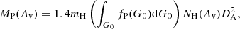
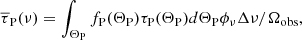
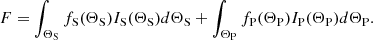
The impact of the density of the pre-shock gas and of the PDRs on the interpretation of observations is shown in Fig. 3a, which displays the minimum distance between the observations and the distribution of shocks and PDR models for a density ranging from 10 to 104 cm−3. The smallest value of the minimum distance is obtained for nH = 10 cm−3, which corresponds to the fiducial model. The corresponding intensities of the 14 emission lines used as constraints predicted by this fiducial model are presented in Fig. 4.
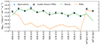 |
Fig. 4. Solution for a combination of shocks and PDRs, assuming an exponential probability distribution function. Solution for the fiducial model nH = 10 cm−3, b = 0.1, G0 = 10 shown in Fig. 3a. Observations are presented as blue stars (see Table B.2) and modeled intensities are shown as open black circles. Individual shock and PDR contributions are shown as green and orange solid lines, respectively. |
As shown in Fig. 4, the combination of shocks and PDRs reproduces all the observational lines by a factor smaller than 2. The H2 lines from 0-0 S(1) to 1-0 S(4) are mostly emitted by shocks. Conversely, the 0-0 S(1) line of H2, the 158 μm line of C+, and the 63 μm line of O are mostly emitted by PDRs.
Figure 3a shows that the minimum distance rapidly increases with the gas density. For instance, a minimum distance larger than ∼1.4 dex is obtained for nH = 103 cm−3, meaning that at most one of the observational lines is underestimated or overestimated by a factor of ∼25. This result is in contradiction with those currently presented in the literature. Fits of the excitation diagram of the H2 pure-rotational transitions with shock models performed by Nesvadba et al. (2010) for 3C 326 N lead to solutions with a density ranging between 103 and 104 cm−3. These discrepancies come from the fact that our observational dataset contains additional constraints, in particular the [CII] 158 μm, and [OI] 63 μm lines. As shown in Fig. D.2, pure shock models cannot reproduce the [OI] line emission, even at low density. Moreover, in Nesvadba et al. (2010) a density of 104 cm−3 was needed to reproduce high-excitation lines (e.g., 0-0 S(7)), but consequently, the 0-0 S(0) line was overpredicted by a factor of ≈2.5. The fact that the [CII] 158 μm line originates from the diffuse gas is in agreement with Guillard et al. (2015b) who found similar results based on the observation of the [CII]-to-FIR ratio in 3C 326 N. It is also in line with Pathak et al. 2024 who recently showed that the diffuse medium has a substantial contribution to the overall emission of the dust in main sequence galaxies.
4.3. Reprocessed radiative and mechanical energies
This new interpretation is valid only if the structures required to explain the observed intensities are in agreement with the energy budget of the source. This sanity check, which is often neglected, is paramount. The method described in Sect. 3.3 allows the computation of the mechanical energy dissipated by shocks ℒK, as well as the UV-reprocessed luminosity in PDRs ℒUV. The resulting luminosities are shown in Fig. 3b as functions of the pre-shock and PDR densities, and compared with the values estimated for 3C 326 N. For the fiducial model (nH = 10 cm−3, b = 0.1, and G0 = 10), we derive a dissipated mechanical power of ℒK = 3.9 × 10⁸ L⊙ and a UV-reprocessed luminosity of ℒUV = 6.3 × 10⁹ L⊙. The mechanical energy dissipated by the shocks is therefore as high as ∼6% of the UV-reprocessed luminosity.
The UV luminosity predicted by the model corresponds to the radiation emitted by OB stars, which is reprocessed by interstellar matter. This radiation is expected to be mostly absorbed by dust and re-emitted at IR wavelengths. To obtain an independent estimate of the amount of UV radiation reprocessed, we performed a fit of the total SED of 3C 326 N, including 14 bands covering the UV-to-FIR range (see Appendix C), using the Bayesian code CIGALE7 (Boquien et al. 2019; Yang et al. 2020, 2022). This treatment leads to a reprocessed UV luminosity LUV = (7.1 ± 1.4)×109 L⊙. This estimate is in agreement with Lanz et al. (2016), and is shown as an orange shaded region in Fig. 3b. This figure displays a remarkable agreement between the UV luminosity derived from the SED and that required to explain the atomic and molecular lines for gas densities ranging between 10–103 cm−3. Interestingly, at nH ≳ 104 cm−3 the UV-reprocessed luminosity obtained with the distribution of shocks and PDRs drops. This is due to the fact that at high densities the 0-0 S(0) line is mainly emitted by low-velocity shocks instead of PDRs.
Estimation of the available mechanical energy is less straightforward. In radio-galaxies, such as 3C 326 N, the interplay between the jet and the ISM results in a transfer of energy and momentum from large scales (the kiloparsec-sized cavities inflated by the AGN-driven outflow, Hardcastle & Croston 2020) to smaller scales through a turbulent cascade, leading to an isotropization of the energy deposited by the AGN feedback, with turbulent velocity dispersions on the order of several hundreds of km s−1 in the diffuse ionized phase (Wittor & Gaspari 2020). This cascade leads to the formation of low-velocity shocks which may account for the dissipation of a substantial fraction of the turbulent mechanical energy in the molecular gas (e.g., Lehmann et al. 2016; Park & Ryu 2019; Richard et al. 2022). According to simulations, approximately 20–30% of the kinetic energy of the jet is deposited into the ISM, depending on the AGN power (e.g., Mukherjee et al. 2016). Most of this energy is used to expand the gas along the jet and to drive gas outflows on subkiloparsec scales (Mukherjee et al. 2018; Morganti et al. 2023; Krause 2023). Recent observations obtained with the JWST suggest that only a minor fraction of this energy (less than 1%) feeds interstellar turbulence (Pereira-Santaella et al. 2022). Nesvadba et al. (2010) estimated a power of the jet of ∼1011 L⊙ from radio observations. The upper limit computed as 1% of this luminosity is shown as a green shaded area in Fig. 3b. For the fiducial model, the kinetic energy reprocessed in low-velocity shocks is found to be in agreement with the small fraction of the mechanical energy of the jet deposited in the ISM in 3C 326 N. Our results confirm that the dissipation of only a small fraction of the kinetic energy of the jet can account for the line emission of molecular hydrogen.
4.4. Total masses and volume of shocks and PDRs
The masses of shocks and PDRs in the fiducial model can be estimated using the prescription described in Sect. 3.4. The typical depth of PDRs is not known, but since the UV-impinging power needs to be entirely reprocessed in IR radiation, the associated visual extinction must be larger than 1. We assume two values of the visual extinction of PDRs, Av = 1 and Av = 10. Using Eqs. (9) and (10), we derive a total mass of shocks, MS = 7.8 × 10⁷ M⊙, and a total mass of PDR, MP = 1.9 × 10⁸ M⊙ (for Av = 1) and MP = 1.9 × 10⁹ M⊙ (for Av = 10). This result implies that between 4 and 40% of the total mass carried by the PDRs is shocked.
This estimation is in agreement with previous estimations of the molecular content of 3C 326 N. Ogle et al. (2007) and Nesvadba et al. (2010) derive a total mass of H2 of 1.1 × 10⁹ M⊙ and 1.3 − 2.7 × 10⁹ M⊙, respectively, from the excitation diagram of H2 observed in 3C 326 N. Similarly, Guillard et al. (2015b) estimate a total molecular mass of ∼2 × 10⁹ M⊙ from the modeling of the FIR emission of dust grains and the emission of the CO(1-0) line.
The volume occupied by the PDRs can be derived from their total surface area and compared with the volume of the galaxy. For the fiducial model (nH = 10 cm−3), we find that the volume of PDRs is comprised between 0.55 kpc3 (for Av = 1) and 5.5 kpc3 (for Av = 10). The volume of the galaxy is uncertain. NIR IFU spectroscopy with the VLT/SINFONI instrument show that the H2 ro-vibrational emission arises from a molecular disk of about 2 kpc in diameter (see Nesvadba et al. 2011, footnote 1 page 3). The IR continuum and optical images show dust emission over 4 kpc (see Fig. 3 in Ogle et al. 2010). In addition, we estimate that the scale height of the galactic disk is between about 0.2 kpc (see Guillard et al. 2015b) and 0.5 kpc (see Fig. 3 in Ogle et al. 2010). This implies that the molecular gas is contained in a volume between 5 and 50 kpc3. These estimations show that the models with densities nH ⩾ 10 cm−3 are coherent because they lead to a volume filling factor smaller than 1. Given the results shown in Fig. 3, the question might arise of why we do not explore gas at densities lower than 10 cm−3. However, this additional constraint shows that such models are ruled out because the molecular gas would occupy a volume larger than that of the galaxy.
4.5. Prediction of the CO(1-0) emission
The observed CO(1-0) emission line intensity given in Table B.1 is not included as a constraint in our model. Low-J CO emission is known to arise from the cold diffuse component of molecular gas (Mingozzi et al. 2018). Given that the total mass of shocks is much lower than that of PDRs, it is therefore expected that the low-J lines of CO are mostly emitted by PDRs.
The distribution of PDRs obtained in the fiducial model leads to a flux of the CO (1-0) line of 6.5 × 10⁻¹⁸ erg s−1 cm−2, a value in fair agreement, yet slightly higher than that observed in 3C 326 N (3.5 × 10⁻¹⁸ erg s−1 cm−2). This result reinforces our interpretation of this galaxy in which the 0-0 S(0), [CII] 158 μm, and [OI] 63 μm lines are mostly emitted by PDRs, while the remaining H2 lines are mostly emitted by shocks.
5. Model predictions for JWST observations
5.1. Impact of shock velocities to the H2 lines
From the fitting of observed line emission in 3C 326 N (Fig. 3), it is clear that H2 lines are mainly powered by shocks, except the lowest excitation 0-0 S(0) line where the PDR contributions dominate. For the fiducial model (nH = 10 cm−3, b = 0.1, and G0 = 10, see Sect. 4), we now investigate, among the distribution of shocks, which shock velocities are the dominant contributors to the emission of H2 lines.
Figure 5 displays the modeled shock integrated line intensities for the suite of 14 emission lines as a function of the shock velocity. A summary of the dominant velocity as a function of the upper-level energy of the H2 lines is presented in Fig. 6. For the lines accessible with JWST observations (i.e., 0-0 S(1) to the 0-0 S(7), and the ro-vibrational 1-0 S(1) to 1-0 S(4)), we show that the dominant shock velocities are remarkably low, in the vs, dom range of 6 km s−1–15 km s−1. The typical length scales over which those shocks dissipate energy is on the order of 0.001–0.01 pc (Kristensen et al. 2023). As previous studies pointed out, this suggests that a small fraction of the feedback kinetic energy cascades to very small scales in the molecular phase, powering the H2 line emission (Nesvadba et al. 2010).
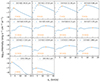 |
Fig. 5. Contributions of the different velocities of the shock distribution to the total intensities emitted by shocks in the fiducial model. The dominant shock velocity vs dom that contributes the most to powering each line is highlighted in orange. Only the range 1–20 km s−1 is shown for readability, even though the models include velocities up to 40 km s−1. |
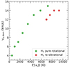 |
Fig. 6. Shock velocity that contributes the most to the H2 line emissions as a function of the upper-level energy (orange points in Fig. 5). H2 pure-rotational (green) and ro-vibrational (red) transitions are presented. vs, dom is derived for the fiducial model nH = 10 cm−3, b = 0.1, and G0 = 10. |
On the more technical side, the shocks responsible for the H2 line emission are J-type shocks, where J stands for jump (see Kristensen et al. 2023, for a discussion of the shock model grid, and in particular their Fig. 6). These shocks are strong emitters of ro-vibrational emission lines, contrary to C-type (continuous) shocks, which were favored in Nesvadba et al. (2010) with fewer observational constraints. Therefore, JWST/NIRSpec observations of 3C 326 N will be a stringent test of our model predictions.
5.2. Impact of the distribution of shock velocities
The impact of the functional form of the distribution of shock velocities is presented in Appendix D.3 where we show the comparison between the model and the observations assuming a Gaussian distribution for fS. Appendix D.3, and in particular Figs. D.3 and D.4, show that a Gaussian distribution leads to the same conclusions regarding the media responsible for the different line emissions and the energy budget required to reproduce the observations. Figure D.3 reveals that assuming a more complex distribution of shock velocities only leads to additional degeneracies. For instance, we find that a narrow distribution of shock velocities centered at μvs = 12 km s−1 leads to the same distance as a broad distribution centered at μvs = 3 km s−1. This implies that the current ensemble of observations is insufficient to discriminate between different distributions of shock velocities as long as the shocks that dominate the ro-vibrational emission of H2 (between 6 and 15 km s−1, see Fig. 5) are included.
5.3. H2 line predictions for JWST
The Paris-Durham shock and the Meudon PDR codes solve for the populations of a large number of H2 levels (see Sect. 2), and therefore provide a predicted spectrum over the entire wavelength range observed by the JWST instruments. Figure 7 displays the spectrum predicted by the fiducial model for the strongest 1000 lines of H2, accounting for the different spectral resolutions of the NIRSpec and MRS spectrographs. We fit the resolving power of the G235H NIRSpec disperser8 over the wavelength range 1.7 − 3.1 μm, finding the resolving power relation R(λ) = 1225λ − 185. For the MIRI instrument, we use the relation R(λ) = 4603 − 128λ reported in Argyriou et al. (2023) valid over the wavelength range 5 − 28 μm. Outside the validity range in wavelength of these relations, we use a uniform resolving power of λ/Δλ = 2500. We note that, although displayed on the synthetic spectrum, the ground-state 0-0 S(0) emission line is not observable with MIRI/MRS because its sensitivity drops above 26.5 μm.
 |
Fig. 7. Predicted synthetic spectrum of H2 in 3C 326 N obtained for the fiducial model (nH = 10 cm−3, b = 0.1, and G0 = 10). The specific intensities of the strongest 1000 emission lines are shown as functions of the redshifted wavelength for z = 0.089. We applied the relations described in Sect. 5.3 for the resolving power of the NIRSpec and MIRI instruments. Outside the validity wavelength range, we fixed the resolving power to a value of λ/Δλ = 2500. The NIRSpec and MIRI bandwidths correspond to the black solid lines. The wide-, medium-, and narrowband filters for NIRCam and MIRI are shown as gray and colored bars. Pure rotation lines are indicated in blue, while ro-vibrational transitions are shown in red and green. |
We predict that the 3C 326 N spectrum should be dominated by ro-vibrational lines with υup = 1 around 2 − 3 μm, as well as the strong 0-0 S(3) and 0-0 S(5) mid-infrared lines. The forest of NIR υup ≥ 1 ro-vibrational lines is thus predicted to be a major cooling channel for the dissipation of kinetic energy.
Luckily, it came to our attention, while this paper was under peer review, that new data obtained with the NIRSpec and MIRI instruments aboard the JWST had just been published (Leftley et al. 2024). These data include 19 H2 lines encompassing S, O, and Q series, as well as the pure-rotational lines 0-0 S(3), 0-0 S(5), and 0-0 S(6). It offered a unique and timely opportunity to test the predictive power of the model. The predictions of the fiducial model were taken as they were and directly compared to these new JWST data. Figure 8 displays the remarkable results that the fiducial model reproduces all the lines observed with the JWST within a factor of about 2. Also, as predicted by Fig. 7, the number of ro-vibrational lines present in the NIRSpec spectrum is abundant and is consistent with an emission powered by the reprocessing of mechanical energy from shocks.
 |
Fig. 8. Comparison of the intensities of the H2 lines predicted by the fiducial model with the new JWST data observed by Leftley et al. 2024, which are corrected here by a factor (1 + z)3 (see Eq. (B.1)). Observations are shown as blue stars and the model predictions as open black circles. We emphasize that the model is obtained by fitting the Spitzer and VLT/SINFONI data, and not the JWST data. |
6. Summary and conclusions
This paper presents a new framework for interpreting atomic and molecular emission lines observed in extragalactic sources. Emission lines collected within an observational beam are assumed to arise from distributions of shocks and PDRs. The comparison of the observations with the predictions of the model leads to the physical properties (e.g., density, UV illumination) of the emitting gas and provides the mechanical and radiative energy budget of the source. As a test case, we selected the radio galaxy 3C 326 N, a unique object with low SFR, large molecular content, and strong IR H2 line emission. A total of 14 emission lines including eight H2 rotational lines from 0-0 S(0) to 0-0 S(7) and four ro-vibrational lines from 1-0 S(1) to 1-0 S(4), as well as [CII] 158 μm and [OI] 63 μm emissions are used as observational constraints.
The framework developed in this paper is an oversimplification of the gas distribution in galaxies. Because the ISM is highly turbulent and contains a distribution of irradiation sources, both the density and G0 should spread over a wide range of values. This diversity of ISM environments is obtained in numerical simulations (e.g., Mukherjee et al. 2018; Murthy et al. 2022) and is derived from the analysis of continuum emission (e.g., Pathak et al. 2024). We designed the model and the underlying distributions to reduce the number of free parameters. This model is not a representation of the actual state of the gas, but rather describes the mean physical conditions of the emitting medium. The remarkable result is that this oversimplified picture already leads to predictions that are in excellent agreement with the observations, and fulfills the constraints on the mechanical and radiative energy budgets. A unique minimum is found with a small degree of degeneracies between the parameters (namely ΩS and σvs). This implies that adopting a distribution of density or G0, while more realistic, would only lead to additional degeneracies. The key results obtained within this framework are summarized as follows:
-
The analysis applied to 3C 326 N shows that the ensemble of observational constraints requires the combined contributions of both a distribution of shocks and a distribution of PDRs within the observational beam.
-
The predictions of the model are found to be highly dependent on the density of the gas and weakly dependent on the other parameters (the ambient radiation field and the magnetic field). Surprisingly, we find that only shocks and PDRs at low density (nH = 10 − 100 cm−3) can reproduce all the observational constraints. This is probably the most salient result of this study. It implies that both the mechanical and UV energy inputs are preferentially reprocessed in the low-density medium of this galaxy.
-
The optimal solution is obtained for nH = 10 cm−3. The likelihood, estimated from the ratios of the observed to the predicted intensities, is characterized by only one global minimum and no local minima. This global minimum provides constraints on the total solid angle of PDRs, the total solid angle of shocks, and the range of shock velocities required to explain the observations. However, the suite of spectral lines used in this work is found to be insufficient to set apart the predictions obtained for an exponential or a Gaussian probability distributions of shock velocities.
-
The H2 0-0 S(0) 28 μm, [CII] 158 μm, and [OI] 63 μm lines are mostly emitted by PDRs. The resulting UV-reprocessed luminosity, ℒUV = 6.3 × 10⁹ L⊙, is found to be in remarkable agreement with the observed IR-luminosity.
-
Conversely, the rest of the H2 lines from the 0-0 S(1) to the 1-0 S(4) are found to be emitted by low-velocity shocks (5 < vs < 20 km s−1). The resulting mechanical luminosity dissipated by shocks, ℒK = 3.9 × 10⁸ L⊙, is less than 1% of the estimated jet kinetic power, in agreement with the predictions of MHD simulations or recent JWST observations.
-
The total mass of shocks is MS = 7.8 × 10⁷ M⊙ and the total mass of PDRs is MP = 1.9 × 10⁹ M⊙. This budget is in line with previous estimations of the molecular content in 3C 326 N and implies that about 4% of the total mass carried by PDRs is shocked.
-
Finally, the predicted synthetic H2 spectrum shows prominent ro-vibrational emission lines, originating from all the vibrational levels of H2. This synthetic spectrum is found to be in excellent agreement with new JWST observations of 3C 326 N, underlining the ability of the model to make accurate predictions.
The new interpretative framework is applied here to a specific source to test the validity and relevance of the underlying method. In a companion paper, we will extend this methodology to a larger sample of objects (see, e.g., Fig. 7 in Guillard et al. 2012 and Fig. 12 in Ogle et al. 2024), such as star-forming galaxies, AGN, radio, or elliptical galaxies, and extract the radiative and mechanical energy budget of these sources from atomic and molecular line emissions.
The fact that most of the reprocessing of the input mechanical and radiative powers occurs in the diffuse gas in 3C 326 N is of particular importance. It remains to be seen whether this result holds for a larger sample of galaxies, which we will explore in a companion paper. It suggests that this methodology should be applied to ancillary interpretations of extragalactic sources. Previous studies (Meijerink et al. 2013; Mingozzi et al. 2018; Esposito et al. 2022) show that PDR and XDR models at high densities (e.g., nH ∼ 104 cm−3) could explain the CO, H2, and [CII] 158 μm emission lines observed toward a few extragalactic sources. It would therefore be interesting to apply our methodology to those sources and estimate whether a combined distribution of shocks, PDRs, and XDRs at low densities could account for the observations with an acceptable energy budget. It is indeed timely because JWST is already observing H2 and fine-structure emission lines in extragalactic sources, in particular in AGN (Pereira-Santaella et al. 2022; Buiten et al. 2024).
Meudon PDR code: https://ism.obspm.fr/pdr.html
Paris-Durham code: https://ism.obspm.fr/shock.html
Available at: http://ism.obspm.fr/index.html
Despite this assumption, the radiative transfer inside each shock and PDR structure is computed taking into account absorption processes.
We do not consider the heating of the molecular gas by the X-ray radiation from the AGN. This is not a strong limitation, as Ogle et al. (2010) showed that the H2–to–X-ray luminosity ratio (> 0.6) is so high that X-ray heating is not a primary driver of H2 line emission.
This choice of typical visual extinction has little impact on the results presented here because the predictions of the shock models regarding H2 emission are insensitive to Av as long as the shocks run in a medium that is mostly molecular (Kristensen et al. 2023).
Available at: https://cigale.lam.fr/
We use the wavelength calibration data from https://jwst-docs.stsci.edu/jwst-near-infrared-spectrograph/nirspec-instrumentation/nirspec-dispersers-and-filters
This approach can easily be expanded to multidimensional distributions. In this paper we assume a distribution of shock velocities, that is ΘS = vS, and a distribution of illumination factors for the PDRs, that is ΘP = G0.
With the adopted cosmology, the 3C 326 redshift of z = 0.089 corresponds to a luminosity distance DL = 422 Mpc, an angular diameter distance DA = 356 Mpc, and a scale of 1.725 kpc/arcsec.
The code is available at: https://cigale.lam.fr/
Acknowledgments
The research leading to these results has received funding from the European Research Council, under the European Community’s Seventh framework Programme, through the Advanced Grant MIST (FP7/2017-2022, No 742719). The grid of simulations used in this work has been run on the computing cluster Totoro of the ERC MIST, administered by MesoPSL. We would also like to acknowledge the support from the Programme National “Physique et Chimie du Milieu Interstellaire” (PCMI) of CNRS/INSU with INC/INP co-funded by CEA and CNES. PG would like to thank the Institut Universitaire de France, the Centre National d’Etudes Spatiales (CNES), and the “Programme National de Cosmologie and Galaxies” (PNCG) of CNRS/INSU, with INC/INP co-funded by CEA and CNES, for their financial supports.
References
- Allen, M. G., Groves, B. A., Dopita, M. A., Sutherland, R. S., & Kewley, L. J. 2008, ApJS, 178, 20 [Google Scholar]
- Almeida, A., Anderson, S. F., Argudo-Fernández, M., et al. 2023, ApJS, 267, 44 [NASA ADS] [CrossRef] [Google Scholar]
- Argyriou, I., Glasse, A., Law, D. R., et al. 2023, A&A, 675, A111 [NASA ADS] [CrossRef] [EDP Sciences] [Google Scholar]
- Begelman, M. C., & Ruszkowski, M. 2005, Phil. Trans. R. Soc. London Ser. A, 363, 655 [Google Scholar]
- Benson, A. J. 2010, Phys. Rep., 495, 33 [NASA ADS] [CrossRef] [Google Scholar]
- Boquien, M., Burgarella, D., Roehlly, Y., et al. 2019, A&A, 622, A103 [NASA ADS] [CrossRef] [EDP Sciences] [Google Scholar]
- Bruzual, G., & Charlot, S. 2003, MNRAS, 344, 1000 [NASA ADS] [CrossRef] [Google Scholar]
- Buiten, V. A., van der Werf, P. P., Viti, S., et al. 2024, ApJ, 966, 166 [NASA ADS] [CrossRef] [Google Scholar]
- Carnall, A. C., McLure, R. J., Dunlop, J. S., & Davé, R. 2018, MNRAS, 480, 4379 [Google Scholar]
- Casey, C. M., Narayanan, D., & Cooray, A. 2014, Phys. Rep., 541, 45 [Google Scholar]
- Chabrier, G. 2003, PASP, 115, 763 [Google Scholar]
- Charlot, S., & Fall, S. M. 2000, ApJ, 539, 718 [Google Scholar]
- Cielo, S., Bieri, R., Volonteri, M., Wagner, A. Y., & Dubois, Y. 2018, MNRAS, 477, 1336 [NASA ADS] [CrossRef] [Google Scholar]
- Ciotti, L., Ostriker, J. P., & Proga, D. 2010, ApJ, 717, 708 [Google Scholar]
- da Cunha, E., Charlot, S., & Elbaz, D. 2008, MNRAS, 388, 1595 [Google Scholar]
- Draine, B. T., Aniano, G., Krause, O., et al. 2014, ApJ, 780, 172 [Google Scholar]
- Esposito, F., Vallini, L., Pozzi, F., et al. 2022, MNRAS, 512, 686 [NASA ADS] [CrossRef] [Google Scholar]
- Ferland, G. J., Chatzikos, M., Guzmán, F., et al. 2017, Rev. Mex. A&A, 53, 385 [Google Scholar]
- Fierlinger, K. M., Burkert, A., Ntormousi, E., et al. 2016, MNRAS, 456, 710 [NASA ADS] [CrossRef] [Google Scholar]
- Flower, D. R., & Pineau des Forêts, G., 1999, MNRAS, 308, 271 [NASA ADS] [CrossRef] [Google Scholar]
- Flower, D. R., & Pineau des Forêts, G., 2003, MNRAS, 343, 390 [Google Scholar]
- Godard, B., Pineau des Forêts, G., Lesaffre, P., et al. 2019, A&A, 622, A100 [NASA ADS] [CrossRef] [EDP Sciences] [Google Scholar]
- Grieco, F., Theulé, P., De Looze, I., & Dulieu, F. 2023, Nat. Astron., 7, 541 [NASA ADS] [CrossRef] [Google Scholar]
- Guillard, P., Boulanger, F., & Pineau des Forêts, G., & Appleton, P. N., 2009, A&A, 502, 515 [NASA ADS] [CrossRef] [EDP Sciences] [Google Scholar]
- Guillard, P., Ogle, P. M., Emonts, B. H. C., et al. 2012, ApJ, 747, 95 [NASA ADS] [CrossRef] [Google Scholar]
- Guillard, P., Boulanger, F., Lehnert, M. D., Appleton, P. N., & Pineau des Forêts, G. 2015a, in SF2A-2015:Proceedings of the Annual meeting of the French Society of Astronomyand Astrophysics, 81 [Google Scholar]
- Guillard, P., Boulanger, F., Lehnert, M. D., et al. 2015b, A&A, 574, A32 [NASA ADS] [CrossRef] [EDP Sciences] [Google Scholar]
- Habart, E., Walmsley, M., Verstraete, L., et al. 2005, Space Sci. Rev., 119, 71 [Google Scholar]
- Hardcastle, M. J., & Croston, J. H. 2020, New A Rev., 88, 101539 [NASA ADS] [CrossRef] [Google Scholar]
- Herrera, C. N., Boulanger, F., Nesvadba, N. P. H., & Falgarone, E. 2012, A&A, 538, L9 [NASA ADS] [CrossRef] [EDP Sciences] [Google Scholar]
- Kim, J.-G., Gong, M., Kim, C.-G., & Ostriker, E. C. 2022, ApJS, 264, 10 [Google Scholar]
- Klessen, R. S., & Hennebelle, P. 2010, A&A, 520, A17 [NASA ADS] [CrossRef] [Google Scholar]
- Krause, M. G. H. 2023, Galaxies, 11, 29 [NASA ADS] [CrossRef] [Google Scholar]
- Kristensen, L. E., Godard, B., Guillard, P., Gusdorf, A., & Pineau des Forêts, G., 2023, A&A, 675, A86 [NASA ADS] [CrossRef] [EDP Sciences] [Google Scholar]
- Krumholz, M. R., Bate, M. R., Arce, H. G., et al. 2014, in Protostars and Planets VI, eds. H. Beuther, R. S. Klessen, C. P. Dullemond, & T. Henning, 243 [Google Scholar]
- Lanz, L., Ogle, P. M., Alatalo, K., & Appleton, P. N. 2016, ApJ, 826, 29 [NASA ADS] [CrossRef] [Google Scholar]
- Leftley, J. H., Nesvadba, N. P. H., Bicknell, G., et al. 2024, A&A, in press, https://doi.org/10.1051/0004-6361/202449848 [Google Scholar]
- Lehmann, A., Federrath, C., & Wardle, M. 2016, MNRAS, 463, 1026 [NASA ADS] [CrossRef] [Google Scholar]
- Lehmann, A., Godard, B., & Pineau des Forêts, G., Vidal-García, A., & Falgarone, E., 2022, A&A, 658, A165 [CrossRef] [EDP Sciences] [Google Scholar]
- Le Petit, F., Nehmé, C., Le Bourlot, J., & Roueff, E. 2006, ApJS, 164, 506 [NASA ADS] [CrossRef] [Google Scholar]
- Lesaffre, P., Pineau des Forêts, G., Godard, B., et al. 2013, A&A, 550, A106 [NASA ADS] [CrossRef] [EDP Sciences] [Google Scholar]
- Lesaffre, P., Todorov, P., Levrier, F., et al. 2020, MNRAS, 495, 816 [NASA ADS] [CrossRef] [Google Scholar]
- Lilly, S. J., & Longair, M. S. 1984, MNRAS, 211, 833 [NASA ADS] [CrossRef] [Google Scholar]
- Mathis, J. S., Mezger, P. G., & Panagia, N. 1983, A&A, 128, 212 [NASA ADS] [Google Scholar]
- Meijerink, R., Kristensen, L. E., Weiß, A., et al. 2013, ApJ, 762, L16 [Google Scholar]
- Mingozzi, M., Vallini, L., Pozzi, F., et al. 2018, MNRAS, 474, 3640 [NASA ADS] [CrossRef] [Google Scholar]
- Morganti, R., Murthy, S., Guillard, P., Oosterloo, T., & Garcia-Burillo, S. 2023, Galaxies, 11, 24 [NASA ADS] [CrossRef] [Google Scholar]
- Mukherjee, D., Bicknell, G. V., Sutherland, R., & Wagner, A. 2016, MNRAS, 461, 967 [NASA ADS] [CrossRef] [Google Scholar]
- Mukherjee, D., Bicknell, G. V., Wagner, A. Y., Sutherland, R. S., & Silk, J. 2018, MNRAS, 479, 5544 [NASA ADS] [CrossRef] [Google Scholar]
- Murthy, S., Morganti, R., Wagner, A. Y., et al. 2022, Nat. Astron., 6, 488 [CrossRef] [Google Scholar]
- Nesvadba, N. P. H., Boulanger, F., Salomé, P., et al. 2010, A&A, 521, A65 [NASA ADS] [CrossRef] [EDP Sciences] [Google Scholar]
- Nesvadba, N. P. H., Boulanger, F., Lehnert, M. D., Guillard, P., & Salome, P. 2011, A&A, 536, L5 [NASA ADS] [CrossRef] [EDP Sciences] [Google Scholar]
- Ogle, P., Antonucci, R., Appleton, P. N., & Whysong, D. 2007, ApJ, 668, 699 [NASA ADS] [CrossRef] [Google Scholar]
- Ogle, P., Boulanger, F., Guillard, P., et al. 2010, ApJ, 724, 1193 [NASA ADS] [CrossRef] [Google Scholar]
- Ogle, P. M., López, I. E., Reynaldi, V., et al. 2024, ApJ, 962, 196 [NASA ADS] [CrossRef] [Google Scholar]
- Ostriker, E. C., & Kim, C.-G. 2022, ApJ, 936, 137 [NASA ADS] [CrossRef] [Google Scholar]
- Park, J., & Ryu, D. 2019, ApJ, 875, 2 [NASA ADS] [CrossRef] [Google Scholar]
- Pathak, D., Leroy, A. K., Thompson, T. A., et al. 2024, AJ, 167, 39 [NASA ADS] [CrossRef] [Google Scholar]
- Pereira-Santaella, M., Álvarez-Márquez, J., García-Bernete, I., et al. 2022, A&A, 665, L11 [NASA ADS] [CrossRef] [EDP Sciences] [Google Scholar]
- Pfenniger, D. 2010, in Galaxies in Isolation: Exploring Nature Versus Nurture, eds. L. Verdes-Montenegro, A. Del Olmo, & J. Sulentic, ASP Conf. Ser., 421, 183 [Google Scholar]
- Planck Collaboration VI. 2020, A&A, 641, A6 [NASA ADS] [CrossRef] [EDP Sciences] [Google Scholar]
- Polles, F. L., Salomé, P., Guillard, P., et al. 2021, A&A, 651, A13 [NASA ADS] [CrossRef] [EDP Sciences] [Google Scholar]
- Richard, T., Lesaffre, P., Falgarone, E., & Lehmann, A. 2022, A&A, 664, A193 [NASA ADS] [CrossRef] [EDP Sciences] [Google Scholar]
- Shaw, G., Ferland, G. J., Henney, W. J., et al. 2009, ApJ, 701, 677 [NASA ADS] [CrossRef] [Google Scholar]
- Stalevski, M., Ricci, C., Ueda, Y., et al. 2016, MNRAS, 458, 2288 [Google Scholar]
- Vazquez-Semadeni, E. 2009, ArXiv e-prints [arXiv:0902.0820] [Google Scholar]
- Willis, A. G., & Strom, R. G. 1978, A&A, 62, 375 [NASA ADS] [Google Scholar]
- Wittor, D., & Gaspari, M. 2020, MNRAS, 498, 4983 [NASA ADS] [CrossRef] [Google Scholar]
- Yang, G., Boquien, M., Buat, V., et al. 2020, MNRAS, 491, 740 [Google Scholar]
- Yang, G., Boquien, M., Brandt, W. N., et al. 2022, ApJ, 927, 192 [NASA ADS] [CrossRef] [Google Scholar]
Appendix A: Conditions of validity of the toy model
The toy model presented in Sect. 3 and used throughout this paper results from a simplification of the radiative transfer of an ensemble of shocks and PDRs within an observational beam. As illustrated in Fig. A.1, we consider that an observational beam of solid angle Ωobs contains shock and PDR surfaces with a distribution of systemic velocities and with total solid angles ΩS and ΩP. For simplicity, we set that the emission from one shock or one PDR in a line with a rest frequency ν0 follows a tophat profile over a width Δν = ν0ΔV/c, with a velocity width ΔV = 5 km s−1 dominated by turbulent motions (Lehmann & Godard 2022). Both shock and PDR surfaces are assumed to have systemic velocities projected along the observed line of sight that follow a Gaussian distribution in frequency space
 (A.1)
(A.1)
 |
Fig. A.1. Schematic representation of ensembles of shocks and PDRs inside an observational beam with a solid angle Ωobs (black and white circle). Shock or PDR surfaces are represented by the filled circles and filled squares, respectively, and are randomly placed within the beam. The color represents the systemic velocities of shock and PDR surfaces projected along the line of sight. Blue (resp. red) circles and squares correspond to blueshifted (resp. redshifted) shocks and PDRs with respect to the recession velocity of the galaxy. The left and right panels represent two equivalent scenarios, where the numbers of shock (resp. PDR) surfaces are different, but subtend the same total solid ΩS (resp. ΩP). This figure is adapted from Lehmann & Godard (2022). |
where  is the observed frequency dispersion of the line. Independently of this distribution, we also assume that ΩS and ΩP follow 1D probability distribution functions, fS(ΘS) and fP(ΘP), which both depend on a unique parameter, ΘS for the shocks and ΘP for the PDRs.9 The solid angles of shock and PDR surfaces that emit within a frequency bin of size Δν centered at a frequency ν therefore write
 (A.2)
(A.2)
and
 (A.3)
(A.3)
The number of shock and PDR layers within a frequency bin or, equivalently, the beam-filling factors per frequency bin of shocks and PDRs are
 (A.4)
(A.4)
and
 (A.5)
(A.5)
Their average total opacities are
 (A.6)
(A.6)
and
 (A.7)
(A.7)
where τS(ΘS) and τP(ΘP) are the opacities across one shock layer of parameter ΘS and one PDR layer of parameter ΘP respectively (see Fig. A.2).
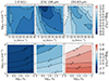 |
Fig. A.2. Opacities of the emission lines in shocks as functions of the pre-shock density and the shock velocity (top row) and in PDRs as a function of the gas density and the illumination factor (bottom row). All other parameters are set to their standard values given in Table 1. The left column is associated with the H2 1-0 S(1) line, the middle column with the [CII] 158 μm line, and the right column with [OI] 63 μm line. The color-coding indicates the central opacity of the lines τS(ν0) and τP(ν0), with a different color scale for shocks and PDRs. |
If there are no spatial overlaps of shocks and PDRs within any frequency bin, that is if
 (A.8)
(A.8)
or if the averaged line opacities across the shock and PDR layers in any frequency bin are small,
 (A.9)
(A.9)
absorption by shocks and PDRs can be neglected. The density flux (in erg cm−2 s−1 Hz−1) collected in the observational beam therefore simply writes
 (A.10)
where  is the specific intensity of the background continuum (in erg s−1 cm−2 Hz−1 sr−1) and IS(ΘS) and IP(ΘP) are the line integrated intensities emitted by one shock of parameter ΘS and one PDR of parameter ΘP, respectively (in erg s−1 cm−2 sr−1). Integrating this equation over frequency finally gives the continuum subtracted line flux (in erg s−1 cm−2)
 (A.11)
This last equation is at the root of the toy model presented in Sect. 3 (Eq. 1). It results from the assumption that the absorption induced by shock and PDR surfaces within the observational beam is negligible. Throughout the paper, we consider that Eq. A.11 is always valid and can be used to find the optimal combination of models that reproduces a given set of observations (see Sect. 4). The validity of this assumption is checked a posteriori by verifying the conditions written in Eqs. A.8 and A.9. The domain of parameters where these conditions break down are highlighted in Figs. 2 and D.3.
Appendix B: The radio galaxy 3C 326 N
3C 326 is a well-known radio source located at z ∼ 0.089 ± 0.001 (Ogle et al. 2007). Optical and IR imaging shows that it is a pair of interacting galaxies, 3C 326 N and 3C 326 S (Fig. 1). We focus on 3C 326 N, centered at α(J2000) =  , δ(J2000) =
 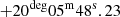 , which hosts the AGN powering the radio jet observed on large scales, with a kinetic luminosity Ljet ∼ 1011 L⊙ (Nesvadba et al. 2010). This galaxy has a remarkably low star formation rate, SFR = (7 ± 3) × 10−2 M⊙ yr−1 (Ogle et al. 2007), yet a large molecular gas content Mgas ∼ 2 × 10⁹ M⊙ (Guillard et al. 2015b). Strong IR H2 line emission has been detected, with a total luminosity L(H2) ≈ 2.4 × 10⁸ L⊙ (Ogle et al. 2007). 3C 326 N represents a perfect target to test which type of physical mechanisms (e.g., shocks and/or PDRs) are responsible for powering the ensemble of H2 lines, while putting constraints on the energy budget of the galaxy. Based on UV GALEX measurements, Ogle et al. (2010) derived a value of G
 for the radiation field in 3C 326 N. Similarly, Guillard et al. (2015b) reported a value of G0 = 9 ± 1 from a fit of the SED in the IR range.
Table B.1 provides a summary of the relevant physical parameters of 3C 326 N.10 The observational solid angle is estimated from the source diameter in optical and IRAC images (Nesvadba et al. 2010). The bulk of the H2 emission is contained inside this beam (Ogle et al. 2010; Nesvadba et al. 2011) as well as the [CII] 158 μm and [OI] 63 μm emissions (Guillard et al. 2015b). The observed fluxes given in Table B.2 are corrected for redshift as
 (B.1)
(B.1)
Observational parameters of 3C 326 N.
and transformed into integrated intensities using the observational solid angle Ωobs. We note that the total observed luminosity of the H2, [CII] 158 μm, and [OI] 63 μm lines is 2.5 × 10⁸ L⊙, which corresponds to about 3% of the IR luminosity and 0.25% of the jet’s luminosity.
B.1. H2 pure rotational and ro-vibrational lines
The observed fluxes and relevant information on the emission lines of molecular hydrogen are given in Table B.2. A total of 12 H2 emission lines have been measured in 3C 326 N. Eight of these are the pure-rotational lines from H2 0-0 S(0) to H2 0-0 S(7), obtained with the mid-infrared Spitzer IRS low-resolution spectroscopy (R ∼ 60 − 120), which did not resolve the lines (Ogle et al. 2010). Four ro-vibrational emission lines, from H2 1-0 S(1) to H2 1-0 S(4), were spatially and spectrally resolved by the VLT/SINFONI spectrograph (Nesvadba et al. 2011). However, since the main goal is to fit the observed integrated intensity of each line, the spectral resolution does not have any impact on our analysis.
Emission line properties of 3C 326 N.
B.2. [CII] 158 μm, [OI] 63 μm, and CO(1-0)
The observed fluxes and relevant information on the emission lines of C+, O, and CO are given in Table B.2. The [CII] 158 μm and the [OI] 63 μm emission lines are taken from observations obtained with Herschel/PACS and reported in Guillard et al. (2015b). The CO(1-0) line intensity is taken from observations performed with the IRAM PdBI and provided by Nesvadba et al. (2010). As explained in the main text, this CO(1-0) emission is not used to constrain the parameters of the model, but is used as a sanity check to test the validity of the solutions obtained.
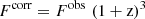
Appendix C: Spectral energy distribution
The SED of 3C 326 N is constrained using the photometric data spanning from the X-ray to the radio bands and available on the NASA/IPAC Extragalactic Database (NED). In this paper we use the measurements of 14 photometric bands obtained, in particular, by Lilly & Longair (1984), Ogle et al. (2010), and Guillard et al. (2015b), and given in Table C.1. These bands include the near-ultraviolet (NUV) GALEX band; the Sloan Digital Sky Surveys u, g, r, i, and z bands (Almeida et al. 2023); and the UKIRT J, UKIRT H, and UKIRT Ks NIR density fluxes. We finally include the Spitzer MIPS 24 μm and MIPS 70 μm bands, the Herschel PACS 100 μm and 160 μm bands, and the Herschel SPIRE 250 μm band.
Photometry of 3C 326 N. The photometric bands derived from the Sloan Digital Sky Surveys (SDSS) were obtained using a circular aperture with a diameter of 8 arcsec on the SDSS DR18 (Almeida et al. 2023).
C.1. SED Fitting
The multiwavelength SED of 3C 326 N covering the UV to FIR range is fitted using the Code Investigating GALaxy Emission (CIGALE11; Boquien et al. 2019; Yang et al. 2020, 2022). CIGALE is based on an energy balance principle where ultraviolet-optical emission is partially absorbed by the dust and subsequently re-emitted in the IR. The code is based on a Bayesian statistical analysis approach that compares millions of models of the panchromatic emission of galaxies with the observations and provides estimates of the mean values and the standard deviations of the physical parameters of the galaxy.
A delayed star formation history without a burst is adopted to model this galaxy based on its low SFR with the simple stellar population models of Bruzual & Charlot (2003) and the initial mass function of Chabrier (2003). We adopt the attenuation law recipe of Charlot & Fall (2000) and the dust IR spectral templates from Draine et al. (2014). In contrast with the results presented in Lanz et al. (2016), we include the IR contribution of the AGN using the SKIRTOR clumpy torus models of Stalevski et al. (2016) and following the configuration reported in Yang et al. (2022) with a fixed opening angle of 40° and varying type-2 viewing angles (θ). All the parameters used for the fit are summarized in Table C.2.
CIGALE modules and input parameters
C.2. Physical parameters: 3C 326 N
Figure C.1 shows the results of the fit of the SED. The black solid line corresponds to the best SED and the different colored lines show the contribution of the stellar, dust, and AGN emission to the overall SED of the galaxy. We obtain a reduced χ2 of 1.2. The Bayesian estimated values of the stellar mass and SFR are presented in Table C.3 with new estimations of the UV and IR luminosities integrated between 0.0912 and 0.24 μm and between 1 and 1000 μm, respectively. The visual attenuation Av and the relative contribution of the AGN to the IR emission fAGN are also reported. The derived stellar mass and SFR are in good agreement (within 30%) with the values reported in the literature (Ogle et al. 2010; Nesvadba et al. 2010; Guillard et al. 2015b). The IR luminosity is also consistent with the fits performed by Guillard et al. (2015b).
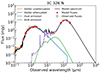 |
Fig. C.1. Spectral energy distribution of 3C 326 N. The MIR-to-FIR photometry is fitted using CIGALE. The stellar attenuated and unattenuated contributions are shown in blue and orange, respectively. The reprocessed IR emission is presented in purple and the AGN emission is in green. The best model is shown as a solid black line. The observed uncertainties are added in quadrature with a 10% floor value to account for possible instrumental errors. |
Physical parameters derived from the fit of the SED.
Appendix D: Alternative scenarios
D.1. PDR-only scenario
We test the possibility of reproducing the ensemble of observations in 3C 326 N using only PDR models. The impact of the PDR density on the interpretation of observations is shown in panel (a) of Fig. D.1, which displays the minimum distance between the observations and the distribution of PDR models for a density ranging from 10 to 104 cm−3. Panel (b) shows the UV-reprocessed luminosity as a function of the density and panel (c) displays the comparisons between the observations and the intensities of the lines predicted by the model at nH = 103 cm−3 (which corresponds to the smallest distance). Figure D.1 shows that PDR-only models cannot explain the observational dataset, and raise two main issues. First, the minimum value of the distance is large (∼2.3). As shown in panel (c), the need to reproduce the observed intensities of all the ro-vibrational lines of H2 leads to overestimations of the intensities of the [CII] 158 μm and [OI] 63 μm lines by one to two orders of magnitude. Second, the predicted UV-reprocessed luminosity is found to be more than one order of magnitude higher than that deduced from the IR luminosity of the galaxy (see panel b). This result demonstrates the importance of estimating the radiative energy budget of galaxies for the interpretation of atomic and molecular emission lines.
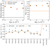 |
Fig. D.1. Summary of the minimum distance, the UV-reprocessed luminosity, and the intensities predicted with a sole distribution of PDR models for the PDR-only scenario. Panel (a): Minimum distance as a function of the gas density. The dashed line represents a 0.5 dex limit (i.e., a factor of three difference between observed and modeled line intensities) to guide the eye. Panel (b): UV-reprocessed luminosity as a function of the gas density. The orange shaded area represents the SED estimation of the reprocessed UV-luminosity (see Appendix C). Panel (c): Comparison between the observed line intensities and those obtained for the model at nH = 103 cm−3, b = 0.1, G0 = 10. The observations are presented as blue stars (see Table B.2) and the modeled intensities are shown as open black circles. In the lower panel, the residuals are shown as orange squares. The dashed and solid lines give the ± 0.5, 1 dex limits, respectively. |
D.2. Shock-only scenario
We also consider the possibility of reproducing all the observations using only shock models. The impact of the density of the pre-shock gas on the interpretation of observations is shown in Fig. D.2 (panel a) which displays the minimum distance between the observations and the distribution of shocks models for a density ranging from 10 to 104 cm−3. Panel (b) shows the mechanical luminosity as a function of the density and panel (c) displays the comparisons between the observations and the intensities of the lines predicted by the model at nH = 10 cm−3 (which corresponds to the smallest distance). Interestingly, the predicted mechanical luminosity is found to be in agreement with the available energy deduced from the jet’s power as long as the density is below 103 cm−3 (see panel b). However, Fig. D.1 shows that a shock-only distribution cannot explain the entire observational dataset. As shown in panel (c), the need to reproduce the observed intensities of the ro-vibrational lines of H2 and of the fine structure line of C+ leads to an underestimation of the [OI] emission by about one order of magnitude. This result demonstrates the importance of including both atomic and molecular lines for the interpretation of extragalactic observations.
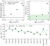 |
Fig. D.2. Summary of the minimum distance, the mechanical luminosity, and the intensities predicted with a sole distribution of shock models for the shock-only scenario. Panel (a): Minimum distance as a function of the pre-shock density. The dashed line represents a 0.5 dex limit (i.e., a factor of three difference between observed and modeled line intensities) to guide the eye. Panel (b): Mechanical luminosity as a function of the pre-shock density. The green area represents < 1% of the estimated jet kinetic luminosity of 3C 326 N (see Sect. 4.3). Panel (c): Comparison between the observed line intensities and those obtained for the model at nH = 10 cm−3, b = 0.1, G0 = 10. Observations are presented as blue stars (see Table B.2) and modeled intensities are shown as open black circles. |
D.3. Gaussian distribution of the shock velocities
We finally explore the impact of the form of the probability distribution function fS assuming that the shock velocities follow a Gaussian distribution
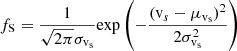 (D.1)
(D.1)
rather than an exponential distribution. Figure D.3 shows the distance computed with Eqs. 3 and 4 as a function of the parameters of the Gaussian distribution of shocks (ΩS, μvs, and σvs) and the parameter of the Dirac distribution of PDRs (ΩP).
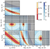 |
Fig. D.3. 2D cutoff of the likelihood distributions of the parameters describing the shock and the PDR distributions obtained for a Gaussian distribution of shock velocities. The parameters are the total shock solid angle ΩS, the central shock velocity μvs and the dispersion of the shock velocities σvs, and the PDR total solid angle ΩP. The color code represents the distance in dex units. The 0.5, 0.7, and 1.0 dex limits are highlighted with dashed black lines. The straight black dashed lines and the black points indicate the position of the global minimum. The gray areas represent the regions where the assumption on the radiative transfer regarding cross-absorption between surfaces breaks down. The criterion is more stringent for the [OI] 63 μm line (gray area above the white solid line) than for the [CII] 158 μm line (gray area above the white dashed line), and is always fulfilled for the H2 lines (see Appendix A). |
The most striking feature of Fig. D.3 is the strong degeneracy between ΩS, μvs, and σvs. A narrow distribution of shock velocities (σvs ∼ 6 km s−1) centered at μvs = 12 km s−1 leads to the same distance as a broad distribution (σvs ∼ 15 km s−1) centered at μvs = 3 km s−1. This strong degeneracy is not surprising and is simply due to the fact that the intensities of the ro-vibrational lines of H2 are mostly emitted by shocks with velocities between 6 and 15 km s−1, regardless of the number of shocks below 6 km s−1 (see Fig. 5).
The impact of the gas density on the interpretation of observations is shown in Fig. D.4 (panel a) which displays the minimum distance between the observations and the distribution of shocks and PDRs for a density ranging from 10 to 104 cm−3. Panel (b) shows the UV-reprocessed luminosity and the mechanical luminosity as functions of the density and panel (c) displays the comparisons between the observations and the intensities of the lines predicted by the model at nH = 10 cm−3 (which corresponds to the smallest distance).
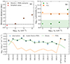 |
Fig. D.4. Summary of the minimum distance, the UV-reprocessed and mechanical luminosities, and the intensities predicted for the PDR and shock scenario with a Gaussian distribution of shock velocities. Panel (a): Minimum distance as a function of the gas density. The dashed line represents a 0.5 dex limit (i.e., a factor of three difference between observed and modeled line intensities) to guide the eye. Panel (b): UV-reprocessed luminosity (orange) and mechanical luminosity (green) as functions of the gas density. The orange shaded area represents the SED estimation of the reprocessed UV-luminosity (see Appendix C). The green area represents < 1% of the estimated jet kinetic luminosity of 3C 326 N (see Sect. 4.3). Panel (c): Comparison between the observed line intensities and those obtained for the model at nH = 10 cm−3, b = 0.1, G0 = 10. The observations are presented as blue stars (see Table B.2) and the modeled intensities are shown as open black circles. |
This ensemble of figures is remarkably similar to those obtained for an exponential distribution of shock velocities (see Fig. 3). In particular, they indicate that the emission likely originates from the diffuse interstellar gas (nH ⩽ 100 cm−3) and that the 0-0 S(0) line of H2 and the fine structure lines of C+ and O are mostly emitted by PDRs, while all the other H2 lines are emitted by shocks, with radiative and mechanical energy budgets in agreement with observational constraints. All these results confirm the interpretation obtained in the main text with an exponential distribution of shock velocities. Figure D.3 reveals that assuming a more complex distribution only leads to additional degeneracies. This means that the current ensemble of observations is insufficient to discriminate between different distributions of shock velocities.
All Tables
Photometry of 3C 326 N. The photometric bands derived from the Sloan Digital Sky Surveys (SDSS) were obtained using a circular aperture with a diameter of 8 arcsec on the SDSS DR18 (Almeida et al. 2023).
All Figures
|
Fig. 1. Schematic representation of the multiphase ISM in a galaxy. Left: radio emission observed in 3C 326 N with the Westerbork Synthesis Radio Telescope (WSRT) 21 cm (Willis & Strom 1978) and Spitzer/IRAC composite image (Ogle et al. 2007) at 3.6, 4.5, and 8.0 μm, showing the 3C 326 N galaxy (and its southern companion). The 3.7″ × 3.7″ (6.4 × 6.4 kpc) square (not-to-scale) represents the solid angle Ωobs over which line emissions are observed. Center: cutout showing the projected proton density from a numerical simulation of the interaction between a radio jet and the central part of a multiphase galactic disk (from Murthy et al. 2022). The different colors show the parsec-scale multiphase structure, with the dense irradiated medium in red (nH ≥ 103 cm−3), the shock diffuse gas in yellow (i.e., nH ∼ 10 − 103 cm−3), and the hot X-ray plasma in green (nH ∼ 1 cm−3). Right: simplified model used in this paper where the observational beam is supposed to encompass distributions of shock and PDR surfaces (see Fig. A.1). |
| In the text | |
|
Fig. 2. 2D cutoff of the likelihood distributions of the main parameters describing the shock and the PDR distributions obtained for the fiducial model. The parameters are the total shock solid angle ΩS, the dispersion of the shock velocities σvs, and the PDR total solid angle ΩP. The color-coding represents the distance in dex units. The 0.5, 0.7, and 1.0 dex limits are highlighted with dashed black lines. The straight black dashed lines and the black points indicate the position of the global minimum. The gray areas represent the regions where the assumption on the radiative transfer regarding cross-absorption between surfaces breaks down. The criterion is more stringent for the [OI] 63 μm line (gray area above the white solid line) than for the [CII] 158 μm line (gray area above the white dashed line), and is always fulfilled for H2 lines (see Appendix A). |
| In the text | |
|
Fig. 3. Solution for a combination of shocks and PDRs, assuming an exponential probability distribution function. Panel (a): distance vs. the medium’s density. The dashed line represents a 0.5 dex limit (i.e., a factor of 3 difference between observed and modeled line intensities) to guide the eye. Panel (b): derived mechanical-reprocessed luminosity from Eq. (6) as well as the UV-reprocessed luminosity from Eq. (8) as a function of density are shown in green and orange, respectively. The green area represents < 1% of the estimated jet kinetic luminosity of 3C 326 N, while the orange area represents the SED estimation of the reprocessed UV-luminosity (see Appendix C). |
| In the text | |
|
Fig. 4. Solution for a combination of shocks and PDRs, assuming an exponential probability distribution function. Solution for the fiducial model nH = 10 cm−3, b = 0.1, G0 = 10 shown in Fig. 3a. Observations are presented as blue stars (see Table B.2) and modeled intensities are shown as open black circles. Individual shock and PDR contributions are shown as green and orange solid lines, respectively. |
| In the text | |
|
Fig. 5. Contributions of the different velocities of the shock distribution to the total intensities emitted by shocks in the fiducial model. The dominant shock velocity vs dom that contributes the most to powering each line is highlighted in orange. Only the range 1–20 km s−1 is shown for readability, even though the models include velocities up to 40 km s−1. |
| In the text | |
|
Fig. 6. Shock velocity that contributes the most to the H2 line emissions as a function of the upper-level energy (orange points in Fig. 5). H2 pure-rotational (green) and ro-vibrational (red) transitions are presented. vs, dom is derived for the fiducial model nH = 10 cm−3, b = 0.1, and G0 = 10. |
| In the text | |
|
Fig. 7. Predicted synthetic spectrum of H2 in 3C 326 N obtained for the fiducial model (nH = 10 cm−3, b = 0.1, and G0 = 10). The specific intensities of the strongest 1000 emission lines are shown as functions of the redshifted wavelength for z = 0.089. We applied the relations described in Sect. 5.3 for the resolving power of the NIRSpec and MIRI instruments. Outside the validity wavelength range, we fixed the resolving power to a value of λ/Δλ = 2500. The NIRSpec and MIRI bandwidths correspond to the black solid lines. The wide-, medium-, and narrowband filters for NIRCam and MIRI are shown as gray and colored bars. Pure rotation lines are indicated in blue, while ro-vibrational transitions are shown in red and green. |
| In the text | |
|
Fig. 8. Comparison of the intensities of the H2 lines predicted by the fiducial model with the new JWST data observed by Leftley et al. 2024, which are corrected here by a factor (1 + z)3 (see Eq. (B.1)). Observations are shown as blue stars and the model predictions as open black circles. We emphasize that the model is obtained by fitting the Spitzer and VLT/SINFONI data, and not the JWST data. |
| In the text | |
|
Fig. A.1. Schematic representation of ensembles of shocks and PDRs inside an observational beam with a solid angle Ωobs (black and white circle). Shock or PDR surfaces are represented by the filled circles and filled squares, respectively, and are randomly placed within the beam. The color represents the systemic velocities of shock and PDR surfaces projected along the line of sight. Blue (resp. red) circles and squares correspond to blueshifted (resp. redshifted) shocks and PDRs with respect to the recession velocity of the galaxy. The left and right panels represent two equivalent scenarios, where the numbers of shock (resp. PDR) surfaces are different, but subtend the same total solid ΩS (resp. ΩP). This figure is adapted from Lehmann & Godard (2022). |
| In the text | |
|
Fig. A.2. Opacities of the emission lines in shocks as functions of the pre-shock density and the shock velocity (top row) and in PDRs as a function of the gas density and the illumination factor (bottom row). All other parameters are set to their standard values given in Table 1. The left column is associated with the H2 1-0 S(1) line, the middle column with the [CII] 158 μm line, and the right column with [OI] 63 μm line. The color-coding indicates the central opacity of the lines τS(ν0) and τP(ν0), with a different color scale for shocks and PDRs. |
| In the text | |
|
Fig. C.1. Spectral energy distribution of 3C 326 N. The MIR-to-FIR photometry is fitted using CIGALE. The stellar attenuated and unattenuated contributions are shown in blue and orange, respectively. The reprocessed IR emission is presented in purple and the AGN emission is in green. The best model is shown as a solid black line. The observed uncertainties are added in quadrature with a 10% floor value to account for possible instrumental errors. |
| In the text | |
|
Fig. D.1. Summary of the minimum distance, the UV-reprocessed luminosity, and the intensities predicted with a sole distribution of PDR models for the PDR-only scenario. Panel (a): Minimum distance as a function of the gas density. The dashed line represents a 0.5 dex limit (i.e., a factor of three difference between observed and modeled line intensities) to guide the eye. Panel (b): UV-reprocessed luminosity as a function of the gas density. The orange shaded area represents the SED estimation of the reprocessed UV-luminosity (see Appendix C). Panel (c): Comparison between the observed line intensities and those obtained for the model at nH = 103 cm−3, b = 0.1, G0 = 10. The observations are presented as blue stars (see Table B.2) and the modeled intensities are shown as open black circles. In the lower panel, the residuals are shown as orange squares. The dashed and solid lines give the ± 0.5, 1 dex limits, respectively. |
| In the text | |
|
Fig. D.2. Summary of the minimum distance, the mechanical luminosity, and the intensities predicted with a sole distribution of shock models for the shock-only scenario. Panel (a): Minimum distance as a function of the pre-shock density. The dashed line represents a 0.5 dex limit (i.e., a factor of three difference between observed and modeled line intensities) to guide the eye. Panel (b): Mechanical luminosity as a function of the pre-shock density. The green area represents < 1% of the estimated jet kinetic luminosity of 3C 326 N (see Sect. 4.3). Panel (c): Comparison between the observed line intensities and those obtained for the model at nH = 10 cm−3, b = 0.1, G0 = 10. Observations are presented as blue stars (see Table B.2) and modeled intensities are shown as open black circles. |
| In the text | |
|
Fig. D.3. 2D cutoff of the likelihood distributions of the parameters describing the shock and the PDR distributions obtained for a Gaussian distribution of shock velocities. The parameters are the total shock solid angle ΩS, the central shock velocity μvs and the dispersion of the shock velocities σvs, and the PDR total solid angle ΩP. The color code represents the distance in dex units. The 0.5, 0.7, and 1.0 dex limits are highlighted with dashed black lines. The straight black dashed lines and the black points indicate the position of the global minimum. The gray areas represent the regions where the assumption on the radiative transfer regarding cross-absorption between surfaces breaks down. The criterion is more stringent for the [OI] 63 μm line (gray area above the white solid line) than for the [CII] 158 μm line (gray area above the white dashed line), and is always fulfilled for the H2 lines (see Appendix A). |
| In the text | |
|
Fig. D.4. Summary of the minimum distance, the UV-reprocessed and mechanical luminosities, and the intensities predicted for the PDR and shock scenario with a Gaussian distribution of shock velocities. Panel (a): Minimum distance as a function of the gas density. The dashed line represents a 0.5 dex limit (i.e., a factor of three difference between observed and modeled line intensities) to guide the eye. Panel (b): UV-reprocessed luminosity (orange) and mechanical luminosity (green) as functions of the gas density. The orange shaded area represents the SED estimation of the reprocessed UV-luminosity (see Appendix C). The green area represents < 1% of the estimated jet kinetic luminosity of 3C 326 N (see Sect. 4.3). Panel (c): Comparison between the observed line intensities and those obtained for the model at nH = 10 cm−3, b = 0.1, G0 = 10. The observations are presented as blue stars (see Table B.2) and the modeled intensities are shown as open black circles. |
| In the text | |
Current usage metrics show cumulative count of Article Views (full-text article views including HTML views, PDF and ePub downloads, according to the available data) and Abstracts Views on Vision4Press platform.
Data correspond to usage on the plateform after 2015. The current usage metrics is available 48-96 hours after online publication and is updated daily on week days.
Initial download of the metrics may take a while.