| Issue |
A&A
Volume 688, August 2024
|
|
|---|---|---|
| Article Number | A212 | |
| Number of page(s) | 14 | |
| Section | Catalogs and data | |
| DOI | https://doi.org/10.1051/0004-6361/202348480 | |
| Published online | 23 August 2024 | |
An extended and refined grid of 3D STAGGER model atmospheres
Processed snapshots for stellar spectroscopy★
1
Stellar Astrophysics Centre, Department of Physics and Astronomy, Aarhus University
Ny Munkegade 120,
8000
Aarhus C,
Denmark
e-mail: This email address is being protected from spambots. You need JavaScript enabled to view it.
2
Department of Astronomy, Stockholm University Albanova University Center,
106 91
Stockholm,
Sweden
3
Theoretical Astrophysics, Department of Physics and Astronomy, Uppsala University,
Box 516,
751 20
Uppsala,
Sweden
4
Université Côte d’Azur, Observatoire de la Côte d’Azur, CNRS,
Lagrange UMR 7293, CS 34229,
06304
Nice Cedex 4,
France
5
DARK, Niels Bohr Institute, University of Copenhagen
Jagtvej 128,
2200
Copenhagen,
Denmark
6
Space Science Institute
4750 Walnut Street, Suite 205,
Boulder,
CO
80301,
USA
Received:
2
November
2023
Accepted:
13
May
2024
Abstract
Context. Traditional one-dimensional hydrostatic model atmospheres introduce systematic modelling errors into spectroscopic analyses of FGK-type stars.
Aims. We present an updated version of the STAGGER-grid of three-dimensional model atmospheres, and explore the accuracy of postprocessing methods in preparation for spectral synthesis.
Methods. New and old models were (re)computed following an updated workflow, including an updated opacity binning technique. Spectroscopic tests were performed in three-dimensional local thermodynamic equilibrium for a grid of 216 fictitious Fe I lines, spanning a wide range of oscillator strengths, excitation potentials, and central wavelengths, and eight model atmospheres that cover the stellar atmospheric parameter range (Teff, log g, and [Fe/H]) of FGK-type stars. Using this grid, the impact of vertical and horizontal resolutions, and temporal sampling of model atmospheres on spectroscopic diagnostics, was tested.
Results. We find that downsampling the horizontal mesh from its original size of 240 × 240 grid cells to 80 × 80 cells, in other words, sampling every third grid cell, introduces minimal errors on the equivalent width and normalised line flux across the line and stellar parameter space. Regarding temporal sampling, we find that sampling ten statistically independent snapshots is sufficient to accurately model the shape of spectral line profiles. For equivalent widths, a subsample consisting of only two snapshots is sufficient, introducing an abundance error of less than 0.015 dex.
Conclusions. We have computed 32 new model atmospheres and recomputed 116 old ones present in the original grid. The public release of the STAGGER-grid contains 243 models and the processed snapshots can be used to improve the accuracy of spectroscopic analyses.
Key words: convection / hydrodynamics / radiative transfer / stars: abundances / stars: atmospheres
© The Authors 2024
 Open Access article, published by EDP Sciences, under the terms of the Creative Commons Attribution License (https://creativecommons.org/licenses/by/4.0), which permits unrestricted use, distribution, and reproduction in any medium, provided the original work is properly cited.
This article is published in open access under the Subscribe to Open model. This email address is being protected from spambots. You need JavaScript enabled to view it. to support open access publication.
1 Introduction
Three-dimensional (3D) compressible radiation-hydrodynamics simulations of stellar atmospheres, known as box-in-a-star models, represent the very essence of stellar atmosphere modelling and thereby spectroscopy for FGK-type stars. After the first studies on solar and stellar granulation and spectral line profiles (Dravins et al. 1981; Nordlund 1982, 1985; Dravins & Nord-lund 1990), the field evolved quickly, with contributions from non-local thermodynamic equilibrium (non-LTE) spectroscopic analyses of the composition of the Sun (Nordlund 1985; Kisel-man & Nordlund 1995; Asplund et al. 2000b, 2003, 2004; Caffau et al. 2008). This led to, among other things, a significant revision of our understanding of the solar chemical composition (Asplund et al. 2009, 2021; Caffau et al. 2011), triggering a debate about the standard model of the Sun that persists to the present day (Serenelli et al. 2009; Christensen-Dalsgaard 2021; Buldgen et al. 2023, 2024).
In addition, 3D atmosphere models coupled with LTE and non-LTE radiative transfer have been applied to determine stellar parameters (Amarsi et al. 2018b; Bonifacio et al. 2018; Bertran de Lis et al. 2022) and stellar abundances in metal-poor stars (e.g. Shchukina et al. 2005; Lind et al. 2013; Amarsi et al. 2016b; Nordlander et al. 2017; Bergemann et al. 2019; Lagae et al. 2023). Grids of 3D LTE (e.g. Chiavassa et al. 2018) and non-LTE spectra are now being calculated (e.g Amarsi et al. 2016a; Mott et al. 2020; Wang et al. 2021) and used to study Galactic chemical evolution and Galactic archaeology for larger samples of stars (e.g. Sbordone et al. 2010; Amarsi et al. 2015, 2019b; Giribaldi et al. 2021,2023). Continuum limb-darkening and centre-to-limb variations of spectral lines have been studied in the Sun with 3D models (e.g. Wedemeyer-Böhm & Rouppe van der Voort 2009; Pereira et al. 2013; Lind et al. 2017), and have been used to constrain atomic data (Amarsi et al. 2018a, 2019a). Furthermore, with the aid of these 3D models, interpolation becomes possible for spectra and limb-darkening coefficients (e.g. Amarsi et al. 2018b; Wang et al. 2021; Bertran de Lis et al. 2022), for equivalent widths and abundance corrections (e.g. Amarsi et al. 2016a, 2019b, 2022; Wang et al. 2021; Gallagher et al. 2016; Harutyunyan et al. 2018; Mott et al. 2020), for photometric corrections (Bonifacio et al. 2018; Chiavassa et al. 2018), and for line shifts and convective blueshifts (Allende Prieto et al. 2013; Chiavassa et al. 2018).
Recent studies have also extended the use of 3D model atmospheres to help with the interpretation of exoplanet transmission spectra (Flowers et al. 2019; Chiavassa & Brogi 2019; Canocchi et al. 2024). Moreover, 3D model atmospheres allow us to accurately model the granulation noise in stars (Rodríguez Díaz et al. 2022), provide an improved theoretical understanding of the properties (e.g. excitation and asymmetry) of pressure-mode oscillations (e.g. Nordlund & Stein 2001; Stein & Nordlund 2001; Georgobiani et al. 2003; Samadi & Goupil 2001; Samadi et al. 2003; Philidet et al. 2020; Belkacem et al. 2021), as well as the so-called ‘surface effect’(Houdek et al. 2017; Trampedach et al. 2017; Sonoi et al. 2019; Zhou et al. 2020, 2021) and calibrate stellar structure models (Trampedach et al. 2014a,b).
The main advantage of 3D model atmospheres over 1D ones is that they do not need parameterised, approximate descriptions of the convective motions and their effects. Convection arises naturally in 3D model atmospheres through heating from the bottom layers. Similarly, radiative cooling near the photosphere leads to the formation of a characteristic granulation pattern, consisting of hot upflows bounded by cool downdrafts. In contrast, 1D models typically invoke mixing-length theory (MLT; Böhm-Vitense 1958) or some variant of it (Canuto & Mazzitelli 1991) to attempt to describe energy transfer due to convection, reproduce temperature gradients in the star’s atmospheres, and influence the properties of spectral lines present in the atmosphere, to name a few examples. This theory cannot fully describe the broadening of spectral lines, or line asymmetries or wavelength shifts, that we observe in stars and that are attributed to stellar surface convection (Dravins et al. 1981). As such, spectroscopic analyses based on one-dimensional (1D) models invoke various other ad hoc parameters, not least so-called microturbulence and macroturbulence, which are assumed to be constants for a given atmosphere, but which turn out to be line-dependent (see more details in e.g. Steffen et al. 2013; Jofré et al. 2014; Slumstrup et al. 2019). In contrast, spectroscopy based on 3D modelling does not need to invoke these parameters (e.g. Asplund et al. 2000b).
An important result from 3D modelling is that the upper atmospheres in 3D models of low-metallicity stars are far cooler than predicted by 1D hydrostatic models in radiative equilibrium (e.g. Asplund et al. 1999). Inefficient radiative cooling in this regime means that the balance between radiative heating and adiabatic cooling is dominated by the latter, which cannot be predicted by 1D models. This can translate to large effects for molecular lines in metal-poor stars, with abundance differences possibly reaching 1 dex (e.g. Collet et al. 2006, 2007; Gallagher et al. 2016).
The major downside of 3D models compared to 1D ones is the increased computational complexity and cost. A symptom of this complexity is the variety of numerical parameters controlling the time step, numerical viscosity, grid size and resolution, and boundary conditions (Asplund et al. 2000a; Grimm-Strele et al. 2015; Collet et al. 2018). The main approximation invoked to deal with the cost is ‘opacity binning’ or multi-group formalism (Nordlund 1982; Skartlien 2000), whereby the radiative heating and cooling rates are computed for just a handful of averaged opacities. The 1D codes, on the other hand, can afford to perform a proper monochromatic opacity sampling, and solve the radiative transfer equation for hundreds of thousands or even millions of individual frequencies. Such a 1D calculation is also needed in order to assign individual wavelengths to bins in the opacity binning method.
Driven by the groundbreaking results above yet hindered by the computational challenges, the construction of extensive grids of 3D model atmospheres is both a necessity and a priority to further advance the field. The CIFIST-grid (Ludwig et al. 2009b; Tremblay et al. 2013) and the STAGGER-grid (Magic et al. 2013a; Stein et al. 2024) reflect this. Both have enabled 3D (non-) LTE spectroscopic analyses of much larger samples of stars as referenced above.
In parallel to these fundamental developments in understanding and modelling of stellar atmospheres, the last 20 years have seen a boom in large stellar surveys. These include photometric missions like CoRoT (Baglin et al. 2006), Kepler (Borucki et al. 2010), and TESS (Ricker et al. 2015), and spectroscopic surveys such as RAVE (Steinmetz et al. 2006), LAMOST (Cui et al. 2012), GALAH (De Silva et al. 2015), Gaia (Gaia Collaboration 2016b), and APOGEE (Majewski et al. 2017). However, 3D model atmospheres have not seen much use in these surveys or in similar stellar surveys - although a notable exception is Gaia Coordination Unit (CU6) (Gaia Collaboration 2016a) and the recent application of the STAGGER-grid to GALAH DR3 (Wang et al. 2024). In the first case, the Gaia/RVS pipeline implemented radial velocity corrections due to convective line-shifts (Asplund et al. 2000b; Chiavassa et al. 2018), by using spectra computed with the STAGGER-grid (Bigot & Thévenin 2008; Chiavassa et al. 2018).
With ever larger stellar surveys on the horizon including 4MOST (de Jong et al. 2019), WEAVE (Jin et al. 2024), and PLATO (Rauer et al. 2014), there is a growing need for extensive grids of 3D model atmospheres. Here we present our efforts to refine and extend the STAGGER-grid, describing our workflow in detail (Sect. 2). We have recomputed 116 models of the original grid, and also computed 32 new models such that the final updated and refined version of the STAGGER-grid contains 243 unique model atmospheres. These models are characterised by their effective temperature (Teff), logarithmic surface gravity (log g), and logarithmic iron abundance relative to the sun ([Fe/H]1). In addition, we discuss how to process these snapshots for stellar spectroscopy applications (Sect. 4), namely, by resampling horizontally and temporally, and by refining the vertical mesh. For the first time, we make a grid of processed snapshots of 3D RHD models available to the community2 (Sect. 5).
2 Method
2.1 The STAGGER-code
In this section, we briefly describe the STAGGER-code. The STAGGER compressible radiation-magnetohydrodynamic (R-MHD) code was originally developed by Nordlund & Galsgaard (1995) – although the grid of models presented in this work does not include magnetic fields – with more recent improvements by Magic et al. (2013a) and Collet et al. (2018), which can be consulted for further details. Additionally, a comprenhen-sive description of the code can be found in Stein et al. (2024). STAGGER solves the time-dependent hydrodynamic equations for the conservation of mass, momentum, and energy, together with the radiative transfer equation assuming LTE. The latter is solved along a total of nine rays, one vertical plus the combination of two inclined polar angles (µ = cos θ) and four azimuthal angles (ϕ-angles), in other words, eighteen directions on the unit sphere (Stein & Nordlund 2003). Computing the full radiative transfer solution for all wavelengths and all grid cells, at every hydrodynamic time step, is computationally unfeasible. Hence, STAGGER employs the opacity binning method (Nordlund 1982; Skartlien 2000; Ludwig & Steffen 2013; Collet et al. 2018) to approximate the full monochromatic problem. In summary, this method associates an average opacity strength with a subsample or ‘bin’ of wavelengths, selected according to their formation depth. The line opacities are taken from Gustafsson et al. (2008) and the sample of continuum absorption and scattering coefficients are taken from Hayek et al. (2010). We used the Mihalas-Hummer-Däppen (MHD) equation of state (EOS) (Mihalas et al. 1988), as it was implemented by (Trampedach et al. 2013). This EOS explicitly includes all ionisation and excitation stages of all included elements, and a realistic treatment of plasma effects on bound states, via the so-called occupation probabilities. All the atomic physics is explicitly calculated for the required abundances, and is identical to that used for the original STAGGER-grid.
In Magic et al. (2013a, Sect. 2.3.2) it was discussed how the wavelengths are sorted into each bin, prioritising a fast and automatic selection of opacity bins for all models, despite the fact that they have different stellar parameters, especially metallic-ities. However, the distribution and limits of the bins directly affect the radiative heating and cooling, which in turn affects the temperature-density stratification of the simulation (Collet et al. 2018). This implies that the automated selection of bin sizes and their boundaries could have an important influence on the models. Therefore, we implemented a new distribution of the 12 bins, chosen because it best replicated the temperature stratification observed in the 48-bin configuration as shown in Collet et al. (2018). An example of the new 12-bin distribution is shown in Fig. 1, where the bin limits are defined by the black lines and have been individually optimised for each model manually.
The differences between the original and the updated opacity binning can be seen in the temperature stratification in the upper atmosphere shown in Fig. 9 in Collet et al. (2018) and will be further discussed in Sect. 2.2.2.
The 3D models generated with the STAGGER-code are of the box-in-a-star type, covering a small region of the stellar atmosphere. Specifically, the box includes the top layers of the convective zone, the super-adiabatic region (SAR), the photosphere, and the upper atmosphere excluding the chromosphere. All models follow a Cartesian geometry with a constant gravity. The horizontal size was specified such that the box contains at least ten granules (see for example Fig. 2). The horizontal boundary conditions are periodic, while the vertical boundaries are transmitting. Specifically, the inflowing gas at the bottom boundary has a constant value of specific entropy per unit mass, s which is specified through the values of density, ρ, and internal energy per mass, є, of the inflows at the bottom (ρbot and ɛbot). The value of sbot(ρbot, ɛbot) does not need to be known3, but is maintained via the first law of thermodynamics:
 (1)
(1)
where ρ is density and є the internal energy, with the gas pressure pth, and temperature, T , calculated from the EOS. The internal energy per unit mass and density are user-specified and model-specific, and directly determine the emergent Teff of the simulation resulting from the complex, non-linear interactions between hydrodynamics, radiative transfer and thermodynamics.
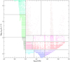 |
Fig. 1 Improved distribution of the 12 opacity bins based on the results of Collet et al. (2018). The Rosseland optical depth at the monochromatic photosphere, τλ = 1, in the average 3D (〈3D〉) reference atmosphere is plotted against the wavelength, where each bin has been assigned a different colour. This representation is for a model with Teff=4500 K, log = 5.0 and [Fe/H]= +0.0. |
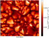 |
Fig. 2 2D colour plot of a snapshot of the bolometric surface intensity of the solar model with dimensions 8 Mm × 8 Mm. |
2.2 Initialising and running a STAGGER model
2.2.1 Initialising a new model
The procedure to start a new 3D stellar atmosphere model was based on similar principles, described in Magic et al. (2013a, see Sect. 2.3.1). The goal is to produce an initial snapshot that is as close to the final, new, relaxed simulation as possible, balanced by the requirements of a robust method that is generally applicable for any late-type stellar atmospheric parameters. This was accomplished with a plane-parallel atmospheric model with adiabatic stratification in (quasi-) hydrostatic equilibrium.
To do so, a relaxed snapshot from another existing 3D model with equal [Fe/H] and close Teff and log g was used, which we refer to as the reference model. The key point is that the reference model should have a similar specific entropy per unit mass at the bottom boundary, as this will determine the emergent Teff of the model. Moreover, a suitable 3D reference model will allow for a better and more efficient scaling and relaxation of a new model (Magic et al. 2013a). Due to the adiabatic nature of the stellar sub-surface convection, the mean entropy in these layers is approximately constant Steffen (1993). Subsequently, from the EOS and the given entropy value at the bottom boundary, an adiabatic density and pressure stratification could be computed, which was in turn used to determine a geometrical depth scale that fulfilled the hydrostatic equilibrium. This resulted in an initial guess for the profiles of the main thermodynamic variables and the geometrical depth scale of the new 3D model, based on the reference model. In addition, the opacity binning scheme of the reference model was copied for the new model, which is refined in a later step (see Sect. 2.2.2). The final initial snapshot is then a plane-parallel atmospheric model with adiabatic stratification in (quasi-) hydrostatic equilibrium.
The horizontal dimensions of the model, l×l, were calculated as follows:
 (2)
(2)
where l⊙ is the horizontal dimension of the solar model. In other words, we re-scaled the horizontal dimensions by an approximate, surface pressure scale height, at constant metallicity. These dimensions are sufficient to capture at least ten granules at any given time. The vertical extent of a new 3D model was chosen to be of the order of ten times the surface pressure scale height and was set on a uniform mesh.
2.2.2 Relaxing a model
Allowing the simulation to settle into its dynamic, but quasi-static ‘natural’ state is known as the relaxation of the simulation. In addition, trying to impose a model with a pre-defined (target) value of the effective temperature demands some adjustments and more iterations, since Teff is an output of the simulation. Hence, a major part of the relaxation process was spent adjusting the bottom boundary conditions to achieve the desired effective temperature. The procedure outlined in this work builds upon the original workflow described in Sect. 2.3 in Magic et al. (2013a).
Step 1. First, we ran the initial snapshot (a ‘low’ grid resolution of 1203) for multiple turnover times with only one vertical ray to compute the radiative heating and cooling rates. We frequently saved snapshots of the model, roughly every Hp/c time, which is the ratio of surface pressure scale height and the sound speed. For the Sun, this value is approximately 20s. This quick first run essentially checks that the simulation allows convective motions to emerge and does not evolve away from quasi-hydrostatic equilibrium.
Step 2. We increased the number of rays used in the radiative transfer solver to three µ = cos θ angles (two inclined and one vertical) and four ϕ-angles. This new set-up provides a more accurate representation of radiative heating and cooling in the atmosphere, without being too computationally expensive Stein & Nordlund (2003). After this change, we ran the simulation for at least three turnover times. Since the radiative transfer is now more accurately treated, the model has a Teff that is close to its true Teff, where true means the one corresponding to the injected heat flux from below (internal energy, density), the gravity and the metallicity.
Step 3. At this point, we checked if the Teff of the model was reasonably close to the target Teff. If yes, then no change of the incoming heat flux was needed. Otherwise, we slightly adjusted the entropy at the bottom by changing the value of either the inflowing internal energy per unit mass or the density at the lower boundary. If the initial model was correctly defined, the change in those quantities had to be small and thereby we assumed that running the model several turnover times is enough to obtain the thermal relaxation. The Kelvin-Helmoltz time that describes this timescale is longer than the turnover time; typically, for the Sun it is roughly a few hours at the depth that corresponds to the bottom of our simulations (e.g. Kupka & Muthsam 2017). Therefore, running a long sequence with many turnover times (≥ 10–20) ensures the thermal equilibrium. In the whole workflow, as is described in this subsection, we reached such duration. The thermal relaxation was nonetheless checked by looking to see if there was any drift in the effective temperature (Fig. 4; see also Sect. 2.3).
Step 4. We proceeded to refine the geometrical depth scale. Initially, the grid points were uniformly distributed in the vertical direction, but to resolve the steep temperature gradients in the SAR, at the moderate mesh resolution used for the STAGGER-grid, more grid points were needed in this region. The idea behind this method is to distribute the mesh points as evenly as possible on the optical-depth scale (Magic et al. 2013a). We suggest that the reader consults Sect. 2.3.1 of Magic et al. (2013a) for details about this step. In contrast to their approach, we no longer automated this step. Instead, the process to refine the geometrical depth scale was done individually and manually for every model, to properly follow the atmospheric stratification of the model, which varies greatly with stellar parameters. An example of a main sequence model and a model in the red giant branch is shown in Fig. 3.
Step 5. To further improve the model, the opacity binning scheme was updated. The overall bin distribution was kept the same, but individual bin boundaries were adjusted as the simulation had reached a new thermal state compared to the initial snapshot. As was mentioned in Sect. 2.1, the opacity binning method was implemented to distribute wavelengths into a small number of groups of bins, each with its own opacity and source function.
To do so, we computed the mean density and temperature stratifications of the model atmosphere, carried out a full monochromatic radiative transfer calculation as a reference case, and perform an optimisation of the bin limits based on the obtained monochromatic heating rates. The optimisation was done for each bin limit individually, where we chose the solution (i.e. the bin boundary location) that resulted in the smallest relative difference between the total heating rates as a result of opacity binning and the full monochromatic solution, as was mentioned in (Magic et al. 2013a, see their Eq. (13)). To obtain the optimal configuration, we iterated over all the bin limits until the position of the bin limits stopped changing.
Step 6. Convective fluctuations excite acoustic modes naturally in the simulation as they do in real stars. However, extra acoustic modes are generated during the relaxation process. They arise in response to changes made to the model (mesh, inflowing internal energy), which in turn adjusts to converge towards its new hydrostatic equilibrium by generating extra pressure perturbations. Since our simulations are very shallow, these acoustic modes have low inertia, and therefore can have sufficiently large amplitudes that can crash the simulations. They need to be damped during the relaxation process. We achieved this by damping the vertical mass flux in the following way:
 (3)
(3)
where 〈…〉 are horizontal averages, py is the vertical component of momentum density, and tdamp is the damping time that corresponds to the period of the fundamental mode. The value depends on the star (Teff, log 𝑔, [Fe/H]) and the vertical extent of the simulation box, and was computed from the Fourier spectrum of the time series of the vertical mass flux during the relaxation stage.
Then, we proceeded to decrease the damping by twice and four times the original value - each time running for only one convective turnover time – so that the box modes of the simulation could emerge at their ‘natural’ amplitude (i.e. the amplitude of the modes of the relax model). Next, we switched the damping off completely and let the simulation run for two convective turnover times.
In the last step, we increased the number of grid points from 120 to 240 in all directions. We ran the model again for several convective turnover times, updated the opacity table and once again damped the box modes. Finally, we initiated the final run of the fully relaxed model, without mode damping, which extended for at least three convective turnover times.
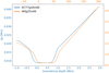 |
Fig. 3 Example of the non-uniform vertical spacing of grid cells for the solar model Teff =5777 K, log = 4.4 and [Fe/H] = +0.0, and a cool giant Teff = 4000 K, log = 2.5 and [Fe/H] = +0.0. |
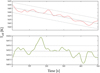 |
Fig. 4 Time evolution of Teff for the same model with Teff = 5500 K, log 𝑔 = 5.0, and [Fe/H] = −4.0. The top panel shows the original non-relaxed model from the grid, with Teff decreasing quite quickly, while the new relaxed model is shown in the bottom panel. The solid grey lines indicate the mean Teff at a given time step, while the dashed lines are spaced out by 1–σ (standard deviation). |
2.3 Criteria for relaxation
In order to check whether a simulation was relaxed, we defined three methods based on earlier work by Magic et al. (2013a) and Trampedach et al. (2013, Sect. 2.4). First, we checked the temporal evolution of the mean bottom boundary internal energy per unit mass and density, effective temperature and box-mode oscillations. While the bottom boundary internal energy per unit mass and density of the upflows are fixed, the mean value, including both downflows and upflows of these quantities at the bottom boundary, can vary slightly due to the convective motions present in the model. If the model is relaxed, the mean bottom boundary internal energy per unit mass and density should fluctuate around a constant value over time. Similarly, the emergent effective temperature should not display a gradient with respect to time. These quick but important checks can immediately show if a model is relaxed or not. An example of this is shown in Fig. 4, where the top panel shows a non-relaxed model, while the bottom one shows a new relaxed version of the same model.
Secondly, we inspected the temporal evolution of several horizontally averaged quantities of a simulation. These include temperature, density, internal energy per unit volume, and vertical and root-mean-square (rms) velocity. These horizontally averaged quantities were computed on layers of constant geometrical and optical depth for all individual snapshots (≈300) of the final run, covering three convective turnover times, following the methodology described in Sect. 4.4. Finally, these quantities were averaged over all snapshots, creating a temporal mean of the full time series. If the model is relaxed, the horizontally averaged quantities of all individual snapshots should be consistent with that of the full time series and there should be no clear trend with respect to time. The latter was checked by comparing the horizontally averaged quantities of the first 20 snapshots to the last 20 snapshots of the simulation.
The third and final step was to inspect the horizontally averaged entropy, to verify that it had a constant value with depth in the convective zone, and verify that hydrostatic equilibrium was fulfilled.
3 An extended and refined STAGGER-grid
3.1 Description of the grid
The original STAGGER-grid computed by Magic et al. (2013a) consisted of 217 models covering a broad range of stellar effective temperatures and surface gravities for seven metallicities. Since its production, the grid has been widely used for several applications, which is a testament to the usefulness, importance, and need for this grid in the astronomical community. Nonetheless, based on the criteria for relaxation discussed in the previous section, some deficiencies were found; namely, multiple model atmospheres showed signs of non-relaxation and a few were missing from the grid. Motivated by this and the need for a grid with more coverage, we have worked on a new version of the STAGGER-grid with fully converged models.
For the majority of the flawed models, relaxation was achieved by running the model for several more convective turnover timescales. Some models required small adjustments to the bottom boundary internal energy, to obtain an effective temperature closer to the target value. Wherever possible, missing models were computed from scratch. Furthermore, we aimed to refine the grid by adding 32 models in the parameter space of particular relevance for upcoming space missions such as PLATO:
Teff = 3500 K, log g = 4.50, [Fe/H] = 0.0
Teff = 4000 K, log g = 4.50, [Fe/H] = 0.0
Teff = 4750 K, log g = 3.25, [Fe/H] = 0.0
Teff = 4750 K, log g = 4.25, all seven metallicities
Teff = 4750 K, log g = 4.75, all seven metallicities
Teff = 5250 K, log g = 4.25, all seven metallicities
Teff = 5250 K, log g = 4.75, all seven metallicities
Teff = 6000 K, log g = 5.00, [Fe/H] = 0.0.
The result of this work is a new extended and refined grid of 3D model atmospheres containing 243 models. Fig. 5 shows an overview of the new grid, where the new and updated models are in green (148), missing or not planned models are in grey, and white represents the unchanged models from the original grid.
The published grid will contain ten snapshots for each model atmosphere, selected using the procedure defined in Sect. 4.4, both in their original format and a processed format that is ready to be used in spectrum synthesis codes. The latter will be discussed in more detail in Sect. 4. Every snapshot contains information on gas temperature, density, internal energy and momentum at each grid point, corresponding to 316 MB or 35 MB memory for both formats, respectively. The mesh information (size and spacing) are stored in two separate files that are provided together with the snapshots. In addition, the EOS is stored in a separate binary file, which can be used to compute additional variables such as the pressure and optical depth at 500 nm. All snapshots, mesh files and complementary analysis scripts are accessible from the new STAGGER website4.
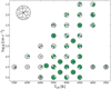 |
Fig. 5 Status of the new and updated STAGGER-grid, where green indicates the new or updated models, grey the missing or not planned models, and white the unchanged models from the original grid. |
3.2 Flagging of peculiar models
In this study, we identified peculiar temperature structures in the outermost layers of both old and new model atmospheres. Specifically, we observed an outward increase in the geometrically and temporally averaged temperatures of several hundred kelvin in the optical thin layers (log τ500 ⪅ − 4)of 31 models. These models are not limited to a certain region of the Hertzsprung-Russell (HR) diagram and range from solar to ultra-metal-poor ([Fe/H] = −4.0). Some heating of the upper atmospheric layers is expected through the energy deposition of acoustic waves generated at the surface by convective motions. Combined with the magnetic fields in the Sun, this gives rise to magneto-acoustic heating of the chromosphere, which is well studied for the Sun (Carlsson & Stein 1992, 1995; Fawzy et al. 2002; Abbasvand et al. 2020; Murawski et al. 2020; Wójcik et al. 2020), but which has gotten limited attention in the case of other stars. For example, Wedemeyer et al. (2017) computed a vertically extended 3D model atmosphere of a red giant star, omitting magnetic fields, using CO5BOLD. Their model developed a highly dynamical chromosphere characterised by acoustic waves evolving into strong shock fronts, heating the gas up to 5000 K. However, these hot regions were not represented in the geometrically averaged temperature stratification, which did not show a significant temperature increase in the chromospheric layers. We observe similar behaviour in the majority of our models that extend into higher atmospheric layers (− 4> log τ500 ⪆ − 10); that is, acoustic waves heating up the gas locally up to 5000–6000 K without a corresponding increase in the mean temperature stratification.
Regarding the 31 models that do show a significant increase in the mean temperature profile, further investigation is required to understand if these layers are a physical or numerical artefact; for example, due to badly constructed opacity binning tables. Regardless, since these ‘chromospheric’ structures occur at small optical depths, we expect no significant impact for most spectroscopic applications such as photospheric line formation. Specifically, for several individual models it was already seen that these layers do not impact spectral line formation and hence could be ignored in subsequent abundance analysis (Lagae et al. 2023). These extremely optically thin layers typically only impact the cores of the strongest lines. Weak metal lines (key diagnostics for chemical compositions, as well as for stellar parameters via excitation and ionisation equilibrium) and the wings of strong lines (important diagnostics of effective temperature and surface gravity) are unaffected. As such, we proceeded to release these models in tandem with the rest of the grid with an added flag (pec_outer) to inform users.
4 Processed snapshots
4.1 Overview
A major hurdle in performing spectrum synthesis in 3D and non-LTE is the computational cost, both in terms of computing time and the memory requirement. The cost of such calculations scales with the size of the model atmosphere NxNYNz times the number of rays, Nray, the number of frequencies, Nv, and the number of iterations, Niter. A simple estimate shows that the computational time of 3D non-LTE spectrum synthesis is at least a factor of 105 larger than corresponding 1D non-LTE calculations (Nordlander et al. 2017; Asplund et al. 2021; Lind & Amarsi 2024). In addition, it is necessary to compute a spectrum for several snapshots of the hydrodynamic simulation to capture the spatial variation in the convective stellar surface. Therefore, it is desirable to post-process the model atmospheres to reduce the computational cost without sacrificing accuracy. In the next subsection, we will go into the details of three methods to post-process model atmospheres and test their corresponding impact on spectral diagnostics using the 3D LTE radiative transfer code Scate (Hayek et al. 2011).
4.2 Trimming
The deep layers of the model atmosphere where the radiation field satisfies Iv ≈ Bv do not contribute to the spectral line formation but do add to the computational cost. Therefore, we can safely cut away these layers prior to performing the radiative transfer calculations. Previous tests to ensure this has minimal effect on the line formation have been performed by Asplund et al. (2000b,a, 2003), Collet et al. (2006) and Amarsi et al. (2016a). In this work we aim to reduce the vertical extent of the models to a size similar to MARCS atmospheres: −5 < log τ < 2 (Gustafsson et al. 2008). However, since every column in the 3D model atmosphere has a different optical depth scale τ(z), we removed all layers with geometrical height, z, that satisfy
 (4)
(4)
and
 (5)
(5)
The resulting atmosphere was then interpolated onto a new grid that was more refined near the optical surface of the star based on the vertical gradient of T4. This new depth scale allows for better accuracy in subsequent radiative transfer calculations and spectral synthesis. As an example, for a random snapshot of the solar simulation, of size 240 × 240 × 240, this procedure removed 118 layers from the bottom and zero layers from the top of the model atmosphere. The remaining 122 layers were then interpolated onto the new depth scale, with a user-specified number of grid points. In the next section, we investigate the effect of interpolating the trimmed atmosphere on the new depth scale, but with a varying number of grid points: 240, 120, and 80.
4.3 Horizontal and vertical grid sampling
The high-resolution STAGGER models were set on a cubic mesh of 240 cells. Such a high resolution is needed in order to resolve features in the simulations when running them, and is therefore crucial for the reliability of any post-processing calculations (Asplund et al. 2000a). With the simulations already established, however, computationally expensive post-processing such as spectral synthesis can greatly benefit from down-sampling the simulations, with little loss in accuracy. For example, 3D non-LTE spectrum synthesis with full-resolution stagger models is unfeasible for large atoms such as Fe due to the excessive computational cost and memory requirements. One possible solution to reduce the computational cost is to downsample the horizontal and vertical mesh while retaining the physical extent of the model atmosphere. This method has been extensively used in previous spectrum synthesis calculations, both 3D LTE (Asplund et al. 2000b; Asplund & García Pérez 2001; Collet et al. 2006; Frebel et al. 2008; Kučinskas et al. 2013) and 3D non-LTE (Asplund et al. 2003; Amarsi et al. 2015, 2016a; Steffen et al. 2015; Bergemann et al. 2019, 2021; Nordlander et al. 2017; Wang et al. 2021; Lagae et al. 2023). Specifically, Nordlander et al. (2017) downsampled a single relaxed STAGGER model to a range of resolutions that were subsequently used in 3D non-LTE spectrum synthesis. They found that downsampling the horizontal mesh of the model atmosphere from 2402 to 602 grid points introduced an error in the equivalent width of less than 0.03 dex. Steffen et al. (2015) found that downsampling the horizontal direction of their 3D solar model by a factor of three resulted in a flux difference of less than 0.1% and an equivalent width error of δWλ/Wλ ≈ 12 × 10−4 for the OI IR triplet. Similarly, Bergemann et al. (2021) study the effect of the horizontal resolution of the solar O I lines in 3D LTE for both a STAGGER and bifrost model atmosphere. They downsampled the original horizontal mesh of size 2402 to 52, 102, 202, 302 and 1202, yielding flux errors less than 2% and abundance errors of 0.01 dex in the case of 302.
In this work, we build on these previous studies by investigating the effect of the horizontal and vertical resolution over a large parameter space. We synthesised a grid of 216 fictitious Fe I lines in 3D LTE covering: log 𝑔f = 0, −1, −2, −3, −4, −5 dex, an excitation potential El = 0−5 eV (∆ = 1eV), and a wavelength of λ = 300–1300 nm (∆ = 200 nm). This grid was computed using Scate for nine different STAGGER models (Table 1) that were trimmed according to Sect. 4.2 and subsequently interpolated to six spatial resolutions (Table 2). The Fe abundance was set to solar (Asplund et al. 2021) or solar-scaled [Fe/H] = -2, depending on the model atmosphere. In these tests, we treated the trimmed and interpolated high-resolution STAGGER model, of size 2402 × 240, as the reference model. To quantify the impact of reducing the horizontal and vertical resolution on the spectral synthesis, we compared the normalised flux and equivalent width of the lower-resolution models to the high-resolution reference model. We limited this analysis to lines that lie on the linear part of the curve of growth,
 (6)
(6)
which we refer to as weak lines, and those lying on the flat part of the curve of growth,
 (7)
(7)
which we refer to as saturated lines in the rest of the paper.
We quantified the impact of the lower-resolution models on the equivalent width by taking the log of the ratio:
 (8)
(8)
as this directly translates into an abundance difference for lines on the linear part of the curve of growth. For the saturated lines, we constructed curve of growths for a single line (λ = 5000 Å, El = 2 eV, log 𝑔f = −4) for all model atmospheres in Table 1 and performed linear regression on the flat part (i.e. −5 < W/λ < −4.5). Since the curve of growth varies depending on the stellar parameters, we adopt the worst case as a uniform relationship between equivalent width and abundance, for all stellar parameters and spectral lines:
 (9)
(9)
The results are visualised in Fig. 6 using box plots for both the saturated and weak lines separately, and six model atmospheres. The box size was set by the first (q1) and third (q3) quartiles, containing 50% of all data points centred around the median. The two whiskers each extend to the smallest and largest data point that are not outliers, with outliers defined as points that are at a distance of >1.5 × (q3 − q1) from the box.
From Fig. 6, we deduce that in general, saturated lines show a larger dependency on resolution. For the saturated lines the abundance error has to be multiplied by a factor of five (see Eq. (9)). However, weak lines become more sensitive to resolution for models at lower metallicity, while the opposite is true for saturated lines. In addition, the error in the equivalent width increases with decreasing surface gravity and increasing stellar effective temperature, as in seen by the large abundance errors for t65g40m20 and t45g20m00. Regarding only weak lines, downsampling the vertical mesh to 120 grid points results in an abundance error of less than 0.02 dex for cool dwarfs and giants. For hotter models such as t65g40m20, the abundance error is at most 0.03 dex. On the other hand, downsampling the horizontal mesh seems to have a minimal impact on the equivalent widths with abundance errors less than 0.007 dex. These results are in line with what has been observed by Steffen et al. (2015), Nordlander et al. (2017), Amarsi & Asplund (2017) and Bergemann et al. (2021).
Next, we investigated the impact of downsampling the mesh on the shape of the normalised line profile. Quantifying the change in line shape is of interest when fitting weak or heavily blended spectral lines, or in the case of transmission spec-troscopy when trying to constrain the presence of planetary spectral features (Canocchi et al. 2024). In addition, constraining the Li isotopic ratio relies critically on the shape of the Li 670.8 nm line itself (Cayrel et al. 2007; Wang et al. 2022). First, the maximum difference in the normalised flux, over the complete line profile, between the downsampled and reference model atmosphere is shown in Fig. 7 for the same lines and model atmospheres discussed above. In this case, the flux difference increases with increasing stellar effective temperature, metal-licity and decreasing surface gravity. Similar to the equivalent widths, stronger lines show larger flux errors compared to weak lines across the stellar parameter space. Moreover, the line profile of weak lines are minimally affected by both the vertical and horizontal resolution with maximum differences in the normalised flux of less than 0.02. In the case of saturated lines, downsampling the vertical mesh to 120 grid points leads to differences in the normalised flux of less than 0.08 for t45g20m00 and less than 0.03 for all other models. Downsampling the horizontal mesh has minimal impact, with typical differences in the normalised flux of less than 0.005 for all model atmospheres. Secondly, the impact of resolution on the shape of the line profile itself is shown in Fig. 8 for two weak and two saturated fictitious Fe I lines with the largest and smallest maximum flux difference, respectively. Downsampling the vertical mesh (red, blue and cyan lines) results in a weaker line core and stronger wings.
From these results, we conclude that, at least for typical applications in stellar spectroscopy, one can safely downsample the horizontal mesh of 3D model atmospheres to 802 × 240, reducing the computational cost by a factor of nine, introducing abundance errors of <0.007 dex and differences in the normalised flux of <0.005. Downsampling both the horizontal and vertical mesh of the model atmosphere to 802 × 120 can be reasonable for certain choices of stellar parameters and spectral lines, such as weak lines in cool dwarfs. However, this only results in an additional factor-two decrease in the computational cost.
Summary of the STAGGER models used in the spatial sampling tests.
Summary of the grid sizes used in the spatial sampling tests.
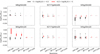 |
Fig. 6 Overview of the relative difference in reduced equivalent width for five different spatial resolutions compared to the reference 2402 × 240 resolution, computed from the 3D LTE flux spectrum. Each box plot contains information from all lines that satisfy the reduced equivalent width requirement shown in the legend. The median of the box plot is represented by a horizontal white line and outliers with a black or red dot. The vertical grey line divides the models with reduced vertical and horizontal resolution. |
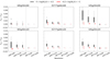 |
Fig. 7 Overview of the maximum difference in normalised flux, over the complete line profile, for five different spatial resolutions compared to the reference 2402 × 240 resolution. Each box plot contains information from all lines that satisfy the reduced equivalent width requirement shown in the legend. The median of the box plot is represented by a horizontal white line and outliers with a black or red dot. The vertical grey line divides the models with reduced vertical and horizontal resolution. |
4.4 Temporal sampling
The 3D simulations only sample a small part of the stellar surface. For example, the stagger solar simulation has a horizontal extent of 8 Mm corresponding to 0.004% of the total surface area. However, stars are observed as point sources and spectral diagnostics are therefore averages over the full stellar disk. Therefore, to accurately model spectral lines, it is necessary to perform spectral synthesis for multiple ‘statistically independent’ snapshots of the simulation, to sample multiple uncorrelated surface granulation patterns of the simulation (Thygesen et al. 2016). In practice, this comes down to performing spectral line calculations for a limited number of snapshots and averaging the resulting line profiles, assuming that the average taken over the sampled snapshots is equivalent to an average over the full stellar disk (Thygesen et al. 2017). The question then becomes, how many snapshots are necessary and how these are selected.
The first tests performed by Asplund et al. (2000a,c) in 3D LTE consisted of computing synthetic line profiles every 30 s for a ‘short’ time series of 10 min solar time. This approach resulted in an abundance error of less than 0.02 dex compared to the full time series.
Later studies expanded on the temporal sampling; for example, by spreading snapshots sufficiently in time for them to be assumed to be statistically uncorrelated (Kučinskas et al. 2013; Thygesen et al. 2016) while simultaneously requiring that the statistical hydrodynamic properties (temperature, density, and velocity) of the subsample resemble that of the full time series (Ludwig et al. 2009b; Kučinskas et al. 2013; Steffen et al. 2015). Subsequent tests by Nordlander et al. (2017) and Wang et al. (2021) in 3D LTE and 3D non-LTE, using equivalent widths, report an abundance error between snapshots of less than 0.03 dex and 0.02 dex, respectively. Other temporal sampling tests include the estimation of effective temperature using Balmer lines (Amarsi et al. 2018b), finding that five snapshots are sufficient to obtain a precision of 10 K. Wang et al. (2022) studied Li, Fe and K lines in three metal-poor dwarf stars, finding that the variation in radial velocity between snapshots in 3D non-LTE is at most 150 m/s and in the best case 7 m/s. Besides these tests, we can summarise the temporal sampling methods used in previous literature work on 3D (non-)LTE spectrum synthesis. Studies with CO5BOLD models, from the CIFIST grid, consistently aim to use 20 snapshots in the analysis (Ludwig et al. 2009b,a; González Hernández et al. 2010; Bonifacio et al. 2010; Caffau et al. 2011; Dobrovolskas et al. 2012, 2013, 2014, 2015; Kučinskas et al. 2013; Siqueira Mello et al. 2013; Klevas et al. 2013; Prakapavičius et al. 2013, 2017; Gallagher et al. 2015, 2016; Steffen et al. 2015; Thygesen et al. 2016, 2017; Černiauskas et al. 2017; Mott et al. 2017; Harutyunyan et al. 2018). On the other hand, studies with STAGGER models usually use between three to five snapshots when performing 3D non-LTE spectrum synthesis (Lind et al. 2013; Amarsi et al. 2015, 2016a, 2018b, 2019b, 2020; Amarsi & Asplund 2017; Nordlander et al. 2017; Lind et al. 2017; Bergemann et al. 2019; Wang et al. 2021, 2022; Lagae et al. 2023; Canocchi et al. 2024) or up to 50 snapshots for 3D LTE spectrum synthesis (Collet et al. 2018; Amarsi et al. 2021). For the purpose of selecting snapshots in the STAGGER grid, we developed a selection method in Python that randomly selects a subsample of Nt snapshots, of which the mean hydrodynamic structure is consistent with that of the complete time series, based on earlier work by Ludwig et al. (2009b), Magic et al. (2013b), Kučinskas et al. (2013) and Steffen et al. (2015). Specifically, we selected a subsample for which the mean vertical stratification, on iso-tau surfaces, of temperature, density, and rms velocity, and the mean of the bolometric surface intensity distribution is consistent with that of the full time series. Here, the rms velocity was calculated as follows:
 (10)
(10)
The mean depth-dependent quantities were first computed for each individual snapshot on horizontal layers of equal optical depth at 500 nm in the range of −5 < log τ500 < 5:
 (11)
(11)
with
 (12)
(12)
and Nx, Ny the number of horizontal grid points. From now on, we shall simply use τ to refer to τ500. Subsequently, the mean quantities were averaged over all of the snapshots in the subsample (Magic et al. 2013b, Sect. 2):
 (13)
(13)
A subsample was deemed acceptable if its mean temperature, density, rms velocity all fell within one standard deviation,  , of the mean quantities of the complete time series:
 (14)
(14)
Here the standard deviation was calculated as follows:
 (15)
(15)
with the sum extending over the full time series. Besides, an additional constraint was placed on each individual snapshot in the subsample to exclude statistical outliers:
 (16)
(16)
In addition, the probability density distribution (PDF) of the bolometric surface intensity at disk centre normalised to its mean value was computed for each subsample and compared to the total time series.
To make sure that the snapshots in each subsample (with Nt > 3) were sampled at different times, to ensure that they were statistically uncorrelated, we enforced a time constraint during the snapshot selection process. Specifically, the method requires that there is at least one snapshot chosen in the following intervals: t < 1/3 ttot, 1/3 ttot < t < 2/3 · ttot, and t > 2/3 ttot, with ttot the total time of the time series. From numerous test runs we conclude that this simple conditions proves sufficient to spread snapshots in time. An example of this selection procedure is shown in Fig. 9 for the STAGGER solar model and a subsample consisting of five snapshots Nt = 5. The mean hydrodynamic quantities from individual snapshots are allowed to deviate from the total mean, but the subsample mean is consistent with the total mean.
Besides the variables mentioned previously, the amplitude of variations around the mean for temperature, density, and rms velocity at every depth layer were also calculated:
 (17)
(17)
where the sum is over all of the grid points, Nx, Ny, in a single layer, with 〈X〉τ the mean quantity of that layer. These variables were not taken into account in the selection method but served as an additional tool with which to review the selected snapshots.
To investigate how many snapshots are necessary to accurately model spectral diagnostics, we selected five subsamples of the solar model (t5777g44m00) consisting of 2, 3, 5, 10 and 20 snapshots respectively, using the selection method discussed previously. For each snapshot in these subsamples, we computed a grid of synthetic spectra, similar to Sect. 4.3. Subsequently, the mean line profile and equivalent width of a subsample were computed by averaging the continuum and line flux separately before normalisation:
 (18)
(18)
with N the number of snapshots in the subsample and F the normalised flux. In the following comparison, we treated the mean normalized flux and equivalent width of all subsamples combined, equal to a total of 40 snapshots, as the reference value.
Figure 10 compares the equivalent width and normalized line flux of the subsample to that of the reference sample. We reiterate that for saturated lines the abundance error has to be multiplied by a factor of five (see Eq. (9)). Subsamples of size N < 10 lead to a maximum abundance error of ≈ 5 × 0.01 dex for saturated lines and ≈0.005 dex for weak lines. Similarly, these subsample sizes show variations of up to 0.015 in the normalised flux of the line compared to the reference spectral line. We conclude that performing an abundance analysis using equivalent widths for weak lines, with at least two suitably selected snapshots, seems sufficient to reach an accuracy smaller than 0.01 dex. On the other hand, to perform an accurate spectral fitting it is advised to use at least ten snapshots corresponding to a maximum difference in the normalised flux of 0.005. For example, such accuracy is necessary to accurately fit the 6Li/7Li line at 6707 Å, which requires residual flux errors lower than ≈0.005 (Mott et al. 2017; Wang et al. 2022).
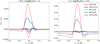 |
Fig. 8 Overview of the relative difference in normalised line profile between the lower-resolution solar models and the reference high-resolution solar model for two weak and two saturated fictitious Fe I lines with the largest and smallest maximum flux difference, respectively. |
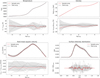 |
Fig. 9 Overview of the subsample selection for the STAGGER model t5777g44m00 of size N = 5. Each panel shows the mean of the total time series (black line), its standard deviation (shaded grey area), the mean of the subsample (red line), and individual snapshots (grey lines), for the variables discussed in the text. From top to bottom and left to right, these are temperature, density, rms velocity, and the normalized probability distribution of surface intensity. |
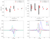 |
Fig. 10 Overview of the relative difference in reduced equivalent width and (maximum) difference in normalised flux for five subsamples compared to the reference sample (N = 40). Each box plot contains information from all lines that satisfy the reduced equivalent width requirement shown in the legend. The bottom two panels show the relative difference in normalised line flux profile between the subsamples and the reference sample for two weak and two saturated fictitious Fe I lines with the largest and smallest maximum flux difference, respectively. |
5 Conclusion
We present an updated version of the STAGGER-grid originally developed by Magic et al. (2013a), in which we have improved the process of scaling, running, and relaxing 3D stellar atmosphere models. The majority of model atmospheres that suffered relaxation problems have been corrected and new dwarf models have been added at intermediate grid points in light of upcoming surveys such as PLATO. This brings the STAGGER-grid to a total of 243 models, excluding all models with [Fe/H] = −4.00 from the original grid, spanning a wide range in Teff, log 𝑔 and metallicity, and covering a large fraction of late-type stars.
Besides updating the STAGGER-grid, we have extensively tested the impact of post-processing procedures such as spatial and temporal sampling, on spectroscopic signatures across a six-dimensional parameter space (Teff, log 𝑔 and [Fe/H], log 𝑔f, E1, λ). These procedures are necessary to make spectrum synthesis feasible in 3D non-LTE. Hence, it is important to characterise their corresponding systematic errors, providing a theoretical basis for future studies. We find that in general, stronger lines in warm evolved stars are the most sensitive to the spatial resolution of model atmospheres. Downsampling the horizontal mesh from 2402 to 802 grid points introduces minimal errors on both abundances of <0.007 dex and fluxes of <0.005, while reducing the computational cost by a factor of nine. Additionally, we find that two snapshots are already sufficient to perform an abundance analysis with equivalent width, introducing a maximum error of 0.01 dex. On the other hand, we recommend using at least ten snapshots when trying to accurately fit line profiles, corresponding to a maximum flux error of 0.005. We remind the reader that these tests have been performed in 3D LTE, although we do expect these results to also be approximately valid in 3D non-LTE. Nevertheless, future studies performing 3D non-LTE spectrum synthesis should investigate the impact of downsampling and temporal sampling in that specific case.
In light of these results, we publicly release ten snapshots for all model atmospheres both in their original format and a downsampled format with mesh dimensions of 802 × 240, occupying 316 MB and 35 MB of memory per snapshot for the two formats, respectively. These snapshots will contribute significantly to several applications in the astronomy community, from spectroscopic studies and abundance determinations to stellar characterization. With upcoming space missions, such as PLATO, the more refined grid will provide even more possibilities for different studies.
Acknowledgements
We thank the anonymous referee for their constructive feedback, which has improved the manuscript. In addition, we thank H.G. Ludwig and B. Freytag for many fruitful discussions and insights on acoustic wave heating in 3D model atmospheres. The numerical results presented in this work were obtained at the Centre for Scientific Computing, Aarhus: https://phys.au.dk/en/research/facilities/centre-for-scientific-computing-aarhus-cscaa. In addition, computational resources were used from the Swedish National Infrastructure for Computing (SNIC) at UPPMAX and the PDC Center for High Performance Computing, partially funded by the Swedish Research Council through grant agreement no. 2018-05973. A.M.A. acknowledges support from the Swedish Research Council (VR 2020-03940). C.L. and K.L. acknowledge funds from the European Research Council (ERC) under the European Union’s Horizon 2020 research and innovation program (Grant Agreement No. 852977). RT acknowledges funding by NASA grants 80NSSC20K0543 and 80NSSC22K0829. This work was supported by the Ministry of Education, Youth and Sports of the Czech Republic through the e-INFRA CZ (ID:90254). This research was supported by computational resources provided by the Australian Government through the National Computational Infrastructure (NCI) under the National Computational Merit Allocation Scheme and the ANU Merit Allocation Scheme (project y89).
References
- Abbasvand, V., Sobotka, M., Švanda, M., et al. 2020, A&A, 642, A52 [EDP Sciences] [Google Scholar]
- Allende Prieto, C., Koesterke, L., Ludwig, H. G., Freytag, B., & Caffau, E. 2013, A&A, 550, A103 [NASA ADS] [CrossRef] [EDP Sciences] [Google Scholar]
- Amarsi, A. M., & Asplund, M. 2017, MNRAS, 464, 264 [Google Scholar]
- Amarsi, A. M., Asplund, M., Collet, R., & Leenaarts, J. 2015, MNRAS, 454, L11 [NASA ADS] [CrossRef] [Google Scholar]
- Amarsi, A. M., Asplund, M., Collet, R., & Leenaarts, J. 2016a, MNRAS, 455, 3735 [NASA ADS] [CrossRef] [Google Scholar]
- Amarsi, A. M., Lind, K., Asplund, M., Barklem, P. S., & Collet, R. 2016b, MNRAS, 463, 1518 [NASA ADS] [CrossRef] [Google Scholar]
- Amarsi, A. M., Barklem, P. S., Asplund, M., Collet, R., & Zatsarinny, O. 2018a, A&A, 616, A89 [NASA ADS] [CrossRef] [EDP Sciences] [Google Scholar]
- Amarsi, A. M., Nordlander, T., Barklem, P. S., et al. 2018b, A&A, 615, A139 [NASA ADS] [CrossRef] [EDP Sciences] [Google Scholar]
- Amarsi, A. M., Barklem, P. S., Collet, R., Grevesse, N., & Asplund, M. 2019a, A&A, 624, A111 [NASA ADS] [CrossRef] [EDP Sciences] [Google Scholar]
- Amarsi, A. M., Nissen, P. E., & Skúladóttir, Á. 2019b, A&A, 630, A104 [NASA ADS] [CrossRef] [EDP Sciences] [Google Scholar]
- Amarsi, A. M., Grevesse, N., Grumer, J., et al. 2020, A&A, 636, A120 [NASA ADS] [CrossRef] [EDP Sciences] [Google Scholar]
- Amarsi, A. M., Grevesse, N., Asplund, M., & Collet, R. 2021, A&A, 656, A113 [NASA ADS] [CrossRef] [EDP Sciences] [Google Scholar]
- Amarsi, A. M., Liljegren, S., & Nissen, P. E. 2022, A&A, 668, A68 [NASA ADS] [CrossRef] [EDP Sciences] [Google Scholar]
- Asplund, M., & García Pérez, A. E. 2001, A&A, 372, 601 [NASA ADS] [CrossRef] [EDP Sciences] [Google Scholar]
- Asplund, M., Nordlund, Å., Trampedach, R., & Stein, R. F. 1999, A&A, 346, L17 [NASA ADS] [Google Scholar]
- Asplund, M., Ludwig, H. G., Nordlund, Å., & Stein, R. F. 2000a, A&A, 359, 669 [NASA ADS] [Google Scholar]
- Asplund, M., Nordlund, Å., Trampedach, R., Allende Prieto, C., & Stein, R. F. 2000b, A&A, 359, 729 [NASA ADS] [Google Scholar]
- Asplund, M., Nordlund, Å., Trampedach, R., & Stein, R. F. 2000c, A&A, 359, 743 [NASA ADS] [Google Scholar]
- Asplund, M., Carlsson, M., & Botnen, A. V. 2003, A&A, 399, L31 [NASA ADS] [CrossRef] [EDP Sciences] [Google Scholar]
- Asplund, M., Grevesse, N., Sauval, A. J., Allende Prieto, C., & Kiselman, D. 2004, A&A, 417, 751 [NASA ADS] [CrossRef] [EDP Sciences] [Google Scholar]
- Asplund, M., Grevesse, N., Sauval, A. J., & Scott, P. 2009, ARA&A, 47, 481 [NASA ADS] [CrossRef] [Google Scholar]
- Asplund, M., Amarsi, A. M., & Grevesse, N. 2021, A&A, 653, A141 [NASA ADS] [CrossRef] [EDP Sciences] [Google Scholar]
- Baglin, A., Auvergne, M., Boisnard, L., et al. 2006, in 36th COSPAR Scientific Assembly, 36, 3749 [Google Scholar]
- Belkacem, K., Kupka, F., Philidet, J., & Samadi, R. 2021, A&A, 646, A5 [NASA ADS] [CrossRef] [EDP Sciences] [Google Scholar]
- Bergemann, M., Gallagher, A. J., Eitner, P., et al. 2019, A&A, 631, A80 [NASA ADS] [CrossRef] [EDP Sciences] [Google Scholar]
- Bergemann, M., Hoppe, R., Semenova, E., et al. 2021, MNRAS, 508, 2236 [NASA ADS] [CrossRef] [Google Scholar]
- Bertran de Lis, S., Allende Prieto, C., Ludwig, H. G., & Koesterke, L. 2022, A&A, 661, A76 [NASA ADS] [CrossRef] [EDP Sciences] [Google Scholar]
- Bigot, L., & Thévenin, F. 2008, in SF2A-2008, eds. C. Charbonnel, F. Combes, & R. Samadi, 3 [Google Scholar]
- Böhm-Vitense, E. 1958, ZAp, 46, 108 [NASA ADS] [Google Scholar]
- Bonifacio, P., Caffau, E., & Ludwig, H. G. 2010, A&A, 524, A96 [NASA ADS] [CrossRef] [EDP Sciences] [Google Scholar]
- Bonifacio, P., Caffau, E., Ludwig, H. G., et al. 2018, A&A, 611, A68 [NASA ADS] [CrossRef] [EDP Sciences] [Google Scholar]
- Borucki, W. J., Koch, D., Basri, G., et al. 2010, Science, 327, 977 [Google Scholar]
- Buldgen, G., Eggenberger, P., Noels, A., et al. 2023, A&A, 669, L9 [NASA ADS] [CrossRef] [EDP Sciences] [Google Scholar]
- Buldgen, G., Noels, A., Baturin, V. A., et al., 2024, A&A, 681, A57 [NASA ADS] [CrossRef] [EDP Sciences] [Google Scholar]
- Caffau, E., Ludwig, H. G., Steffen, M., et al. 2008, A&A, 488, 1031 [CrossRef] [EDP Sciences] [Google Scholar]
- Caffau, E., Ludwig, H. G., Steffen, M., Freytag, B., & Bonifacio, P. 2011, Sol. Phys., 268, 255 [Google Scholar]
- Canocchi, G., Lind, K., Lagae, C., et al. 2024, A&A, 683, A242 [NASA ADS] [CrossRef] [EDP Sciences] [Google Scholar]
- Canuto, V. M., & Mazzitelli, I. 1991, ApJ, 370, 295 [NASA ADS] [CrossRef] [Google Scholar]
- Carlsson, M., & Stein, R. F. 1992, ApJ, 397, L59 [Google Scholar]
- Carlsson, M., & Stein, R. F. 1995, ApJ, 440, L29 [Google Scholar]
- Cayrel, R., Steffen, M., Chand, H., et al. 2007, A&A, 473, L37 [NASA ADS] [CrossRef] [EDP Sciences] [Google Scholar]
- Černiauskas, A., Kucinskas, A., Klevas, J., et al. 2017, A&A, 604, A35 [NASA ADS] [CrossRef] [EDP Sciences] [Google Scholar]
- Chiavassa, A., & Brogi, M. 2019, A&A, 631, A100 [NASA ADS] [CrossRef] [EDP Sciences] [Google Scholar]
- Chiavassa, A., Casagrande, L., Collet, R., et al. 2018, A&A, 611, A11 [NASA ADS] [CrossRef] [EDP Sciences] [Google Scholar]
- Christensen-Dalsgaard, J. 2021, Living Rev. Solar Phys., 18, 2 [Google Scholar]
- Collet, R., Asplund, M., & Trampedach, R. 2006, ApJ, 644, L121 [NASA ADS] [CrossRef] [Google Scholar]
- Collet, R., Asplund, M., & Trampedach, R. 2007, A&A, 469, 687 [NASA ADS] [CrossRef] [EDP Sciences] [Google Scholar]
- Collet, R., Nordlund, Å., Asplund, M., Hayek, W., & Trampedach, R. 2018, MNRAS, 475, 3369 [NASA ADS] [CrossRef] [Google Scholar]
- Cui, X.-Q., Zhao, Y.-H., Chu, Y.-Q., et al. 2012, Res. Astron. Astrophys., 12, 1197 [Google Scholar]
- de Jong, R. S., Agertz, O., Berbel, A. A., et al. 2019, The Messenger, 175, 3 [NASA ADS] [Google Scholar]
- De Silva, G. M., Freeman, K. C., Bland-Hawthorn, J., et al. 2015, MNRAS, 449, 2604 [NASA ADS] [CrossRef] [Google Scholar]
- Dobrovolskas, V., Kucinskas, A., Andrievsky, S. M., et al. 2012, A&A, 540, A128 [NASA ADS] [CrossRef] [EDP Sciences] [Google Scholar]
- Dobrovolskas, V., Kucinskas, A., Steffen, M., et al. 2013, A&A, 559, A102 [NASA ADS] [CrossRef] [EDP Sciences] [Google Scholar]
- Dobrovolskas, V., Kucinskas, A., Bonifacio, P., et al. 2014, A&A, 565, A121 [NASA ADS] [CrossRef] [EDP Sciences] [Google Scholar]
- Dobrovolskas, V., Kucinskas, A., Bonifacio, P., et al. 2015, A&A, 576, A128 [NASA ADS] [CrossRef] [EDP Sciences] [Google Scholar]
- Dravins, D., & Nordlund, A. 1990, A&A, 228, 203 [NASA ADS] [Google Scholar]
- Dravins, D., Lindegren, L., & Nordlund, A. 1981, A&A, 96, 345 [NASA ADS] [Google Scholar]
- Fawzy, D., Rammacher, W., Ulmschneider, P., Musielak, Z. E., & Stepien, K. 2002, A&A, 386, 971 [NASA ADS] [CrossRef] [EDP Sciences] [Google Scholar]
- Flowers, E., Brogi, M., Rauscher, E., Kempton, E. M. R., & Chiavassa, A. 2019, AJ, 157, 209 [Google Scholar]
- Frebel, A., Collet, R., Eriksson, K., Christlieb, N., & Aoki, W. 2008, ApJ, 684, 588 [NASA ADS] [CrossRef] [Google Scholar]
- Gaia Collaboration (Brown, A. G. A., et al.) 2016a, A&A, 595, A2 [NASA ADS] [CrossRef] [EDP Sciences] [Google Scholar]
- Gaia Collaboration (Prusti, T., et al.) 2016b, A&A, 595, A1 [NASA ADS] [CrossRef] [EDP Sciences] [Google Scholar]
- Gallagher, A. J., Ludwig, H. G., Ryan, S. G., & Aoki, W. 2015, A&A, 579, A94 [NASA ADS] [CrossRef] [EDP Sciences] [Google Scholar]
- Gallagher, A. J., Caffau, E., Bonifacio, P., et al. 2016, A&A, 593, A48 [NASA ADS] [CrossRef] [EDP Sciences] [Google Scholar]
- Georgobiani, D., Stein, R. F., & Nordlund, Å. 2003, ApJ, 596, 698 [CrossRef] [Google Scholar]
- Giribaldi, R. E., da Silva, A. R., Smiljanic, R., & Cornejo Espinoza, D. 2021, A&A, 650, A194 [NASA ADS] [CrossRef] [EDP Sciences] [Google Scholar]
- Giribaldi, R. E., Van Eck, S., Merle, T., et al. 2023, A&A, 679, A110 [NASA ADS] [CrossRef] [EDP Sciences] [Google Scholar]
- González Hernández, J. I., Bonifacio, P., Ludwig, H. G., et al. 2010, A&A, 519, A46 [NASA ADS] [CrossRef] [EDP Sciences] [Google Scholar]
- Grimm-Strele, H., Kupka, F., Löw-Baselli, B., et al. 2015, New A, 34, 278 [NASA ADS] [CrossRef] [Google Scholar]
- Gustafsson, B., Edvardsson, B., Eriksson, K., et al. 2008, A&A, 486, 951 [NASA ADS] [CrossRef] [EDP Sciences] [Google Scholar]
- Harutyunyan, G., Steffen, M., Mott, A., et al. 2018, A&A, 618, A16 [NASA ADS] [CrossRef] [EDP Sciences] [Google Scholar]
- Hayek, W., Asplund, M., Carlsson, M., et al. 2010, A&A, 517, A49 [NASA ADS] [CrossRef] [EDP Sciences] [Google Scholar]
- Hayek, W., Asplund, M., Collet, R., & Nordlund, Å. 2011, A&A, 529, A158 [NASA ADS] [CrossRef] [EDP Sciences] [Google Scholar]
- Houdek, G., Trampedach, R., Aarslev, M. J., & Christensen-Dalsgaard, J. 2017, MNRAS, 464, L124 [Google Scholar]
- Jin, S., Trager, S. C., Dalton, G. B., et al. 2024, MNRAS, 530, 2688 [NASA ADS] [CrossRef] [Google Scholar]
- Jofré, P., Heiter, U., Soubiran, C., et al. 2014, A&A, 564, A133 [NASA ADS] [CrossRef] [EDP Sciences] [Google Scholar]
- Kiselman, D., & Nordlund, A. 1995, A&A, 302, 578 [Google Scholar]
- Klevas, J., Ludwig, A. K. H. G., Bonifacio, P., & Steffen, M. 2013, Mem. Soc. Astron. Ital. Suppl., 24, 78 [Google Scholar]
- Kupka, F., & Muthsam, H. J. 2017, Living Rev. Computat. Astrophys., 3, 1 [CrossRef] [Google Scholar]
- Kučinskas, A., Steffen, M., Ludwig, H. G., et al. 2013, A&A, 549, A14 [Google Scholar]
- Lagae, C., Amarsi, A. M., Rodríguez Díaz, L. F., et al. 2023, A&A, 672, A90 [NASA ADS] [CrossRef] [EDP Sciences] [Google Scholar]
- Lind, K., & Amarsi, A. M. 2024, ARA&A, submitted [arXiv:2401.00697] [Google Scholar]
- Lind, K., Melendez, J., Asplund, M., Collet, R., & Magic, Z. 2013, A&A, 554, A96 [NASA ADS] [CrossRef] [EDP Sciences] [Google Scholar]
- Lind, K., Amarsi, A. M., Asplund, M., et al. 2017, MNRAS, 468, 4311 [NASA ADS] [CrossRef] [Google Scholar]
- Ludwig, H. G., & Steffen, M. 2013, Mem. Soc. Astron. Ital. Suppl., 24, 53 [Google Scholar]
- Ludwig, H. G., Behara, N. T., Steffen, M., & Bonifacio, P. 2009a, A&A, 502, L1 [NASA ADS] [CrossRef] [EDP Sciences] [Google Scholar]
- Ludwig, H. G., Caffau, E., Steffen, M., et al. 2009b, Mem. Soc. Astron. Italiana, 80, 711 [NASA ADS] [Google Scholar]
- Magic, Z., Collet, R., Asplund, M., et al. 2013a, A&A, 557, A26 [NASA ADS] [CrossRef] [EDP Sciences] [Google Scholar]
- Magic, Z., Collet, R., Hayek, W., & Asplund, M. 2013b, A&A, 560, A8 [NASA ADS] [CrossRef] [EDP Sciences] [Google Scholar]
- Majewski, S. R., Schiavon, R. P., Frinchaboy, P. M., et al. 2017, AJ, 154, 94 [NASA ADS] [CrossRef] [Google Scholar]
- Mihalas, D., Dappen, W., & Hummer, D. G. 1988, ApJ, 331, 815 [NASA ADS] [CrossRef] [Google Scholar]
- Mott, A., Steffen, M., Caffau, E., Spada, F., & Strassmeier, K. G. 2017, A&A, 604, A44 [NASA ADS] [CrossRef] [EDP Sciences] [Google Scholar]
- Mott, A., Steffen, M., Caffau, E., & Strassmeier, K. G. 2020, A&A, 638, A58 [EDP Sciences] [Google Scholar]
- Murawski, K., Musielak, Z. E., & Wójcik, D. 2020, ApJ, 896, L1 [NASA ADS] [CrossRef] [Google Scholar]
- Nordlander, T., Amarsi, A. M., Lind, K., et al. 2017, A&A, 597, A6 [NASA ADS] [CrossRef] [EDP Sciences] [Google Scholar]
- Nordlund, A. 1982, A&A, 107, 1 [Google Scholar]
- Nordlund, A. 1985, in NATO Advanced Study Institute (ASI) Series C, Vol. 152, Progress in Stellar Spectral Line Formation Theory, eds. J. E. Beckman, & L. Crivellari, 215 [Google Scholar]
- Nordlund, Å., & Galsgaard, K. 1995, A 3D MHD code for Parallel Computers, Tech. rep. Niels Bohr Institute, University of Copenhagen [Google Scholar]
- Nordlund, Å., & Stein, R. F. 2001, ApJ, 546, 576 [Google Scholar]
- Pereira, T. M. D., Asplund, M., Collet, R., et al. 2013, A&A, 554, A118 [NASA ADS] [CrossRef] [EDP Sciences] [Google Scholar]
- Philidet, J., Belkacem, K., Samadi, R., Barban, C., & Ludwig, H. G. 2020, A&A, 635, A81 [NASA ADS] [CrossRef] [EDP Sciences] [Google Scholar]
- Prakapavičius, D., Steffen, M., Kucinskas, A., et al. 2013, Mem. Soc. Astron. Ital. Suppl., 24, 111 [Google Scholar]
- Prakapavičius, D., Kucinskas, A., Dobrovolskas, V., et al. 2017, A&A, 599, A128 [NASA ADS] [CrossRef] [EDP Sciences] [Google Scholar]
- Rauer, H., Catala, C., Aerts, C., et al. 2014, Exp. Astron., 38, 249 [Google Scholar]
- Ricker, G. R., Winn, J. N., Vanderspek, R., et al. 2015, J. Astron. Telescopes Instrum. Syst., 1, 014003 [Google Scholar]
- Rodríguez Díaz, L. F., Bigot, L., Aguirre Børsen-Koch, V., et al. 2022, MNRAS, 514, 1741 [CrossRef] [Google Scholar]
- Samadi, R., & Goupil, M. J. 2001, A&A, 370, 136 [NASA ADS] [CrossRef] [EDP Sciences] [Google Scholar]
- Samadi, R., Nordlund, Å., Stein, R. F., Goupil, M. J., & Roxburgh, I. 2003, A&A, 404, 1129 [NASA ADS] [CrossRef] [EDP Sciences] [Google Scholar]
- Sbordone, L., Bonifacio, P., Caffau, E., et al. 2010, A&A, 522, A26 [NASA ADS] [CrossRef] [EDP Sciences] [Google Scholar]
- Serenelli, A. M., Basu, S., Ferguson, J. W., & Asplund, M. 2009, ApJ, 705, L123 [Google Scholar]
- Shchukina, N. G., Trujillo Bueno, J., & Asplund, M. 2005, ApJ, 618, 939 [NASA ADS] [CrossRef] [Google Scholar]
- Siqueira Mello, C., Spite, M., Barbuy, B., et al. 2013, A&A, 550, A122 [NASA ADS] [CrossRef] [EDP Sciences] [Google Scholar]
- Skartlien, R. 2000, ApJ, 536, 465 [NASA ADS] [CrossRef] [Google Scholar]
- Slumstrup, D., Grundahl, F., Silva Aguirre, V., & Brogaard, K. 2019, A&A, 622, A111 [NASA ADS] [CrossRef] [EDP Sciences] [Google Scholar]
- Sonoi, T., Ludwig, H. G., Dupret, M. A., et al. 2019, A&A, 621, A84 [NASA ADS] [CrossRef] [EDP Sciences] [Google Scholar]
- Steffen, M. 1993, in ASP Conf. Ser., 40, IAU Colloq. 137: Inside the Stars, eds. W. W. Weiss, & A. Baglin, 300 [Google Scholar]
- Steffen, M., Caffau, E., & Ludwig, H. G. 2013, Mem. Soc. Astron. Ital. Suppl., 24, 37 [Google Scholar]
- Steffen, M., Prakapavicius, D., Caffau, E., et al. 2015, A&A, 583, A57 [NASA ADS] [CrossRef] [EDP Sciences] [Google Scholar]
- Stein, R. F., & Nordlund, Å. 2001, ApJ, 546, 585 [Google Scholar]
- Stein, R. F., & Nordlund, Å. 2003, in ASP Conf. Ser., 288, Stellar Atmosphere Modeling, eds. I. Hubeny, D. Mihalas, & K. Werner, 519 [Google Scholar]
- Stein, R. F., Nordlund, Å., Collet, R., & Trampedach, R. 2024, ApJ, accepted [arXiv:2405.02483] [Google Scholar]
- Steinmetz, M., Zwitter, T., Siebert, A., et al. 2006, AJ, 132, 1645 [Google Scholar]
- Thygesen, A. O., Sbordone, L., Ludwig, H. G., et al. 2016, A&A, 588, A66 [NASA ADS] [CrossRef] [EDP Sciences] [Google Scholar]
- Thygesen, A. O., Kirby, E. N., Gallagher, A. J., et al. 2017, ApJ, 843, 144 [CrossRef] [Google Scholar]
- Trampedach, R., Asplund, M., Collet, R., Nordlund, Å., & Stein, R. F. 2013, ApJ, 769, 18 [NASA ADS] [CrossRef] [Google Scholar]
- Trampedach, R., Stein, R. F., Christensen-Dalsgaard, J., Nordlund, Å., & Asplund, M. 2014a, MNRAS, 442, 805 [NASA ADS] [CrossRef] [Google Scholar]
- Trampedach, R., Stein, R. F., Christensen-Dalsgaard, J., Nordlund, Å., & Asplund, M. 2014b, MNRAS, 445, 4366 [CrossRef] [Google Scholar]
- Trampedach, R., Aarslev, M. J., Houdek, G., et al. 2017, MNRAS, 466, L43 [Google Scholar]
- Tremblay, P. E., Ludwig, H. G., Freytag, B., Steffen, M., & Caffau, E. 2013, A&A, 557, A7 [NASA ADS] [CrossRef] [EDP Sciences] [Google Scholar]
- Wang, E. X., Nordlander, T., Asplund, M., et al. 2021, MNRAS, 500, 2159 [Google Scholar]
- Wang, E. X., Nordlander, T., Asplund, M., et al. 2022, MNRAS, 509, 1521 [Google Scholar]
- Wang, E. X., Nordlander, T., Buder, S., et al. 2024, MNRAS, 528, 5394 [CrossRef] [Google Scholar]
- Wedemeyer, S., Kucinskas, A., Klevas, J., & Ludwig, H.-G. 2017, A&A, 606, A26 [NASA ADS] [CrossRef] [EDP Sciences] [Google Scholar]
- Wedemeyer-Böhm, S., & Rouppe van der Voort, L. 2009, A&A, 503, 225 [NASA ADS] [CrossRef] [EDP Sciences] [Google Scholar]
- Wójcik, D., Kuzma, B., Murawski, K., & Musielak, Z. E. 2020, A&A, 635, A28 [NASA ADS] [CrossRef] [EDP Sciences] [Google Scholar]
- Zhou, Y., Asplund, M., Collet, R., & Joyce, M. 2020, MNRAS, 495, 4904 [CrossRef] [Google Scholar]
- Zhou, Y., Nordlander, T., Casagrande, L., et al. 2021, MNRAS, 503, 13 [NASA ADS] [CrossRef] [Google Scholar]
Defined as: [A/B] = log10(NA/NB)★ − log10(NA/NB)⊙ where NA and NB are the number densities of element A and B, respectively.
The specific entropy is computed as an integration of (∂s/∂ ln ρ)ε = −pgas/(ρT) along isochores in the EOS table, but is not needed for running simulations.
STAGGER-website: https://3dsim.oca.eu
All Tables
All Figures
|
Fig. 1 Improved distribution of the 12 opacity bins based on the results of Collet et al. (2018). The Rosseland optical depth at the monochromatic photosphere, τλ = 1, in the average 3D (〈3D〉) reference atmosphere is plotted against the wavelength, where each bin has been assigned a different colour. This representation is for a model with Teff=4500 K, log = 5.0 and [Fe/H]= +0.0. |
| In the text | |
|
Fig. 2 2D colour plot of a snapshot of the bolometric surface intensity of the solar model with dimensions 8 Mm × 8 Mm. |
| In the text | |
|
Fig. 3 Example of the non-uniform vertical spacing of grid cells for the solar model Teff =5777 K, log = 4.4 and [Fe/H] = +0.0, and a cool giant Teff = 4000 K, log = 2.5 and [Fe/H] = +0.0. |
| In the text | |
|
Fig. 4 Time evolution of Teff for the same model with Teff = 5500 K, log 𝑔 = 5.0, and [Fe/H] = −4.0. The top panel shows the original non-relaxed model from the grid, with Teff decreasing quite quickly, while the new relaxed model is shown in the bottom panel. The solid grey lines indicate the mean Teff at a given time step, while the dashed lines are spaced out by 1–σ (standard deviation). |
| In the text | |
|
Fig. 5 Status of the new and updated STAGGER-grid, where green indicates the new or updated models, grey the missing or not planned models, and white the unchanged models from the original grid. |
| In the text | |
|
Fig. 6 Overview of the relative difference in reduced equivalent width for five different spatial resolutions compared to the reference 2402 × 240 resolution, computed from the 3D LTE flux spectrum. Each box plot contains information from all lines that satisfy the reduced equivalent width requirement shown in the legend. The median of the box plot is represented by a horizontal white line and outliers with a black or red dot. The vertical grey line divides the models with reduced vertical and horizontal resolution. |
| In the text | |
|
Fig. 7 Overview of the maximum difference in normalised flux, over the complete line profile, for five different spatial resolutions compared to the reference 2402 × 240 resolution. Each box plot contains information from all lines that satisfy the reduced equivalent width requirement shown in the legend. The median of the box plot is represented by a horizontal white line and outliers with a black or red dot. The vertical grey line divides the models with reduced vertical and horizontal resolution. |
| In the text | |
|
Fig. 8 Overview of the relative difference in normalised line profile between the lower-resolution solar models and the reference high-resolution solar model for two weak and two saturated fictitious Fe I lines with the largest and smallest maximum flux difference, respectively. |
| In the text | |
|
Fig. 9 Overview of the subsample selection for the STAGGER model t5777g44m00 of size N = 5. Each panel shows the mean of the total time series (black line), its standard deviation (shaded grey area), the mean of the subsample (red line), and individual snapshots (grey lines), for the variables discussed in the text. From top to bottom and left to right, these are temperature, density, rms velocity, and the normalized probability distribution of surface intensity. |
| In the text | |
|
Fig. 10 Overview of the relative difference in reduced equivalent width and (maximum) difference in normalised flux for five subsamples compared to the reference sample (N = 40). Each box plot contains information from all lines that satisfy the reduced equivalent width requirement shown in the legend. The bottom two panels show the relative difference in normalised line flux profile between the subsamples and the reference sample for two weak and two saturated fictitious Fe I lines with the largest and smallest maximum flux difference, respectively. |
| In the text | |
Current usage metrics show cumulative count of Article Views (full-text article views including HTML views, PDF and ePub downloads, according to the available data) and Abstracts Views on Vision4Press platform.
Data correspond to usage on the plateform after 2015. The current usage metrics is available 48-96 hours after online publication and is updated daily on week days.
Initial download of the metrics may take a while.