| Issue |
A&A
Volume 688, August 2024
|
|
|---|---|---|
| Article Number | A188 | |
| Number of page(s) | 17 | |
| Section | Interstellar and circumstellar matter | |
| DOI | https://doi.org/10.1051/0004-6361/202346955 | |
| Published online | 20 August 2024 | |
Gas phase Elemental abundances in Molecular cloudS (GEMS)
X. Observational effects of turbulence on the chemistry of molecular clouds
1
Departamento de Estadística e Investigación Operativa, Facultad de Ciencias Matemáticas, Universidad Complutense de Madrid,
Spain
e-mail: This email address is being protected from spambots. You need JavaScript enabled to view it.
2
Centro de Astrobiología (CAB), CSIC-INTA,
Ctra. de Ajalvir Km. 4, Torrejón de Ardoz,
28850
Madrid,
Spain
3
Université Paris-Saclay, Université Paris Cité, CEA, CNRS, AIM,
91191
Gif-sur-Yvette,
France
4
Joint Center for Ultraviolet Astronomy, Universidad Complutense de Madrid,
Avda Puerta de Hierro s/n,
28040
Madrid,
Spain
5
Sección Departamental, Departamento de Física de la Tierra y Astrofísica, Facultad de Ciencias Matemáticas, Universidad Complutense de Madrid,
Plaza de Ciencias 3,
28040
Madrid,
Spain
6
Laboratoire d’astrophysique de Bordeaux, Univ. Bordeaux, CNRS,
B18N, allée Geoffroy Saint-Hilaire,
33615
Pessac,
France
7
Centre for Astrochemical Studies, Max-Planck-Institute for Extraterrestrial Physics,
Giessenbachstrasse 1,
85748
Garching,
Germany
8
Institut de Planétologie et d’Astrophysique de Grenoble (IPAG), Université Grenoble Alpes, CNRS,
38000
Grenoble,
France
9
Institut de Radioastronomie Millimétrique (IRAM),
300 Rue de la Piscine,
38406
Saint-Martin-d’Hères,
France
10
Observatorio Astronómico Nacional (OAN, IGN),
Alfonso XII, 3,
28014
Madrid,
Spain
11
Instituto de Física Fundamental (CSIC),
Calle Serrano 121-123,
28006
Madrid,
Spain
Received:
19
May
2023
Accepted:
7
June
2024
Abstract
Context. We explore the chemistry of the most abundant C-, O-, S-, and N-bearing species in molecular clouds, in the context of the IRAM 30 m Large Programme Gas phase Elemental abundances in Molecular Clouds (GEMS). Thus far, we have studied the impact of the variations in the temperature, density, cosmic-ray ionisation rate, and incident UV field in a set of abundant molecular species. In addition, the observed molecular abundances might be affected by turbulence which needs to be accounted for in order to have a more accurate description of the chemistry of interstellar filaments.
Aims. In this work, we aim to assess the limitations introduced in the observational works when a uniform density is assumed along the line of sight for fitting the observations, developing a very simple numerical model of a turbulent box. We searched for any observational imprints that might provide useful information on the turbulent state of the cloud based on kinematical or chemical tracers.
Methods. We performed a magnetohydrodynamical (MHD) simulation in order to reproduce the turbulent steady state of a turbulent box with properties typical of a molecular filament before collapse. We post-processed the results of the MHD simulation with a chemical code to predict molecular abundances, and then post-processed this cube with a radiative transfer code to create synthetic emission maps for a series of rotational transitions observed during the GEMS project.
Results. From the kinematical point of view, we find that the relative alignment between the observer and the mean magnetic field direction affect the observed line profiles, obtaining larger line widths for the case when the line of sight is perpendicular to the magnetic field. These differences might be detectable even after convolution with the IRAM 30 m efficiency for a nearby molecular cloud. From the chemical point of view, we find that turbulence produces variations for the predicted abundances, but they are more or less critical depending on the chosen transition and the chemical age. When compared to real observations, the results from the turbulent simulation provides a better fit than when assuming a uniform gas distribution along the line of sight.
Conclusions. In the view of our results, we conclude that taking into account turbulence when fitting observations might significantly improve the agreement with model predictions. This is especially important for sulfur bearing species which are very sensitive to the variations of density produced by turbulence at early times (0.1 Myr). The abundance of CO is also quite sensitive to turbulence when considering the evolution beyond a few 0.1 Myr.
Key words: astrochemistry / magnetohydrodynamics (MHD) / turbulence / ISM: clouds
© The Authors 2024
 Open Access article, published by EDP Sciences, under the terms of the Creative Commons Attribution License (https://creativecommons.org/licenses/by/4.0), which permits unrestricted use, distribution, and reproduction in any medium, provided the original work is properly cited.
This article is published in open access under the Subscribe to Open model. This email address is being protected from spambots. You need JavaScript enabled to view it. to support open access publication.
1 Introduction
Molecular clouds are highly turbulent (Hennebelle & Falgarone 2012; Heyer & Brunt 2004) and although the nature of this turbulence is not fully understood, it seems to be a mixture of solenoidal (divergence-free) and compressive (curl-free) modes, where the contribution of each mode depends on the local conditions (Federrath et al. 2010): regions with a low star-formation rate seem to be dominated by solenoidal modes, while massive star-forming complexes with strong feedback present a non-negligible contribution of compressive modes. Despite our limited knowledge on the properties of turbulence, it has been put forward many times as a likely explanation for unexpected observational results. For instance, Tokuda et al. (2018) found structures in molecular gas that were thought to be caused by supersonic turbulence. One of the most puzzling findings was the high abundance of some molecular species in the diffuse phase of the interstellar medium (ISM, Crane et al. 1995; Lucas & Liszt 1996; Neufeld et al. 2012), where according to the predictions of chemical models they should not be able to survive. In order to determine why this occurred, some theories have been developed based on the intermittency of turbulence (Godard et al. 2014) that aim at linking the properties of turbulence with the observations. More recently, the advent of modern computation has made it possible to follow the chemical evolution of the diffuse phase in 3D magnetohydrodynamical (MHD) simulations, either simultaneously to the MHD evolution (Franeck et al. 2018; Moseley et al. 2021) or in a post-processing stage (Myers et al. 2015; Bisbas et al. 2017; Bialy et al. 2019; Godard et al. 2023).
The simultaneous study of the chemical and dynamical evolution of molecular clouds has a huge potential that only recently has been able to be exploited thanks to the widespread access to supercomputers. Generally speaking, there are three alternatives for coupling chemistry and MHD simulations. The first one relies on the implementation of a reduced chemical network where only a set of species is followed (Seifried et al. 2017b; Katz 2022). Depending on the problem to be studied, the number of species varies and specific chemical networks can be selected for particular cases, for instance, for the study of deuterium frac-tionation in turbulent cloud cores (Körtgen et al. 2017; Hsu et al. 2021), for the chemistry in star-forming filaments (Seifried & Walch 2016), or for assessing the reliability of determining filament masses and widths from CO emission maps (Seifried et al. 2017a). A second approach consists of post-processing a numerical simulation with a chemistry code, which is less expensive in terms of computation time. This technique has proved to be useful for tasks such as the calibration of the HCN-star formation correlation (Onus et al. 2018) or the analysis of the interface of colliding molecular clouds (Bisbas et al. 2017). Finally, the third approach that is also computationally expensive but allows the chemo-dynamical evolution of the gas to be solved relies on evolving a set of tracer particles that store the local properties of the gas at fixed times that can be later post-processed with chemical codes (Hincelin et al. 2013, 2016; Coutens et al. 2020; Ferrada-Chamorro et al. 2021; Navarro-Almaida et al. 2024).
It is extremely complicated to establish a direct link between observations and predictions from numerical models; a recent example is the work by Koch et al. (2017), where they introduce several statistical tracers that can be used for the comparison of simulations and observations; however, when applied to real datasets they obtained nonconclusive results. In this article, we present a detailed analysis of the observational effects of turbulence as predicted by a simple MHD model of a molecular cloud that we post-processed with a chemical model plus a radiative transfer code to analyse the predicted chemical variations of the main set of molecules observed during the IRAM 30 m Large Programme Gas phase Elemental abundances in Molecular cloudS (GEMS; Fuente et al. 2019, 2023; Navarro-Almaida et al. 2020; Rodríguez-Baras et al. 2021; Bulut et al. 2021; Spezzano et al. 2022; Esplugues et al. 2022). First, in Sect. 2 we present the setup of the MHD simulation. Then, in Sect. 3 we give the details on the chemistry and radiative transfer codes used for post-processing the simulations in order to derive chemical abundances. The results are presented in the following sections focussing on: (i) the kinematic tracers in Sect. 4, with a special focus on the effects on the spectral line profiles; and (ii) the effects on the estimated chemical abundances (Sect. 5). In Sect. 6 we provide a comparison between our predictions and a subset of the full GEMS observational sample, and in Sect. 7 we discuss the limitations of the paper. Finally, in Sect. 8 we provide the conclusions of our work.
2 MHD model
Ideally, we would like to simulate the evolution of a molecular cloud from the moment of its formation up to the point where star formation might occur, just before collapse, taking into account all the physics and chemistry involved. However, this kind of simulation is highly expensive in terms of computational time and requires implementing a reduced chemical network that reproduces properly the abundances of the main sulfur reservoirs, which does not exist at this point. Therefore, the aim of this paper was to develop a very simple numerical model that allowed us to assess the extent of the influence of turbulence on real single-dish observations. In particular, our goal was to analyse the results of these simulations in the context of the GEMS project. Therefore, although numerical models without chemistry can be generalised and do not have an inherent physical scale unless some microphysics is included, we wanted to choose the parameters such as they could be representative of the interior of a low-mass star formation filament such as the Taurus molecular cloud, which we have extensively studied in previous papers of the GEMS series. If we were to model a molecular filament of width 0.5 pc, according to the following equation (Hacar et al. 2023):
 (1)
(1)
corresponds to a particle density of n = 2.57 × 104 cm−3, and a magnetic field strength of 92.60 µG (B = 10 µG (n/300 cm−3)0.5, Tritsis et al. 2015). In principle, modelling the MHD evolution of such filament is trivial, but in a post-processing stage we are aiming to recover molecular line emission maps for the transitions observed in GEMS. Considering that the nominal resolution of IRAM 30 m telescope for most of the transitions observed in GEMS is around 25″, for the case of a nearby cloud at the distance of Taurus (~ 140 pc, Loinard et al. 2007) roughly corresponds to 0.01 pc. For the study of observational dilution effects of small scale turbulent patches we consider that in order to derive robust statistical estimates, we need to average at least 20 cells per beam so that we reproduce the same ‘loss’ of resolution than observations, and therefore the optimal resolution for the simulation would be 10243 cells, which is highly expensive in terms of computer time for both the MHD simulation and the post-processing stage with radiative transfer. Instead, we opted for performing small scale simulations (box size of 0.05 pc and numerical resolution of 2563) representative of a portion of the full filament. Depending on the observed frequency, this box contains 2–3 beams of the IRAM 30 m telescope assuming the distance of Taurus. This resolution, although quite low for standard MHD turbulence models, is enough to account for the observational effects since we will be averaging the density values contained in a beam. This, of course, will bias our study to large-scale density fluctuations as discussed in Sect. 7.
For the MHD model, we adopt the turbulent-box approximation. This framework is very common for studying turbulent mixing in the ISM (Bialy et al. 2017; Moseley et al. 2021, Godard et al. 2023) and assumes a medium initially at rest in which turbulence is injected over time via a forcing source. In this paper, we use the Athena++1 (Stone et al. 2020) MHD code, with a second-order Van-Leer time integrator, the Harten-Lax-van Leer-Discontinuities (HLLD) Riemann solver and second-order spatial reconstruction (Picewise-Linear-Mesh, PLM). In the current public version of Athena++, a turbulence driver based on the Ornstein-Uhlenbeck process (Lynn et al. 2012) is implemented; the full details of this implementation can be found in Lynn et al. (2012), but we will provide here a simple explanation for the general reader. In a nutshell, the turbulence driver injects velocity ‘kicks’ through a velocity perturbation which amplitude is chosen randomly in the Fourier space normalised by a decreasing power-law in k, ensuring that the majority of the energy is injected in the largest scale, which is L/2, where L is the domain length. This random velocity field which is injected in the domain allows for a combination of solenoidal and compressive modes, and the net energy input can be also controlled so that the desired turbulent Mach number is achieved.
In this initial exploratory work, we assumed an isothermal medium that evolves according to the equations of ideal MHD. Although this approach is rather simplistic because we are ignoring the ion-neutral drift and assuming no heating or cooling effects, this model can be regarded as a starting point for estimating the effects of turbulence in the predicted molecular abundances of a molecular filament; in a future work, we will refine it including more physics as well as active chemistry. Besides, as pointed out by Bialy et al. (2017) for moderate mach numbers (𝓜 ≲ 5) the gas distribution for isothermal and non-isothermal simulations is similar, and since observations of non-fragmenting molecular filaments are compatible with a roughly transonic state (Hacar et al. 2023), we can safely adopt these assumptions as long as we keep in mind that the estimates will be somewhat limited; we discuss the current limitations of our model in Sect. 7.
As we have already mentioned, the MHD simulations are scale-free and the main parameters could be chosen based on the required Mach number, the plasma β parameter, and some characteristic length. However, in order to provide an easier guide for observers and to ensure that the environment is as representative for Taurus as possible, we set up the numerical parameters based on physical quantities for gas density, temperature and box length. We assume that we have an isothermal medium at T = 12 K, n = 2.57 × 104 cm−3 and a box size of L = 0.05 pc at a resolution of 2563 with periodic boundary conditions. We choose a wavenumber for the turbulent spectrum between 2π/L and 4π/L following a power law P(k) ∝ k−2, and assuming a scenario where we have both solenoidal and compressive modes in the same proportion (mixed turbulence). This is a reasonable assumption since Taurus is a low-mass star formating region, and compressive turbulence is more characteristic of high-mass star forming regions, but we cannot discard the presence of some shock waves propagating in the cloud due to former stellar feedback. In any case, in Sect. 7 we discuss the differences between this model of mixed turbulence with other similar ones with different turbulent mixing modes and magnetic field strengths, which are negligible.
We start from a uniform medium at rest with magnetic field parallel to the x-axis and a strength of B0 = 40 µG which is less than the roughly 90 µG predicted by Tritsis et al. (2015), but compatible with observations (see Fig. 5 in Hacar et al. 2023). In order to reproduce the steady-state of a real cloud, we continuously drive turbulence until equilibrium is reached between injection and dissipation rates, which typically occurs after two crossing times, where we define tcross = L/2cs𝓜 as in Federrath (2013) and Lane et al. (2022), and we let the simulation to evolve for three crossing times, resulting in a trans-sonic turbulent box evolved for roughly 0.36 Myr with velocity dispersions of the order of 0.23 km s−1 (see Fig. 1), comprised in the range 0.1–0.5 km s−1 typical of Taurus (Dobashi et al. 2018). The resulting density and velocity probability density functions (PDFs) are shown in Fig. 1. In the density PDF, the values range from 0.06n0 and 5.95n0, where n0 = 2.57 × 104 cm−3 is the initial molecular hydrogen density. Other important quantities that will be used later in the paper are the 1.5% and 98.5% percentiles, which correspond to P1.5 = 0.27n0 and P98.5 = 2.41n0. We want to note that in our simulation, the mean direction of the magnetic field barely changes due to turbulence (mean deviation of 1.5circ), providing a scenario coherent with Taurus observations reporting that the magnetic field is relatively uniform in scales of pc and roughly perpendicular to the molecular filaments (Messinger et al. 1997; Chapman et al. 2011). The apparent differences in the velocity PDFs are not physical but a consequence of the moderate numerical resolution.
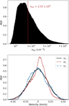 |
Fig. 1 Density and velocity probability density functions (PDFs) at the final stage of the simulation (~0.36 Myr). |
3 Chemical models and post-processing
As in previous GEMS works (Navarro-Almaida et al. 2020, hereafter GEMS II; Rodríguez-Baras et al. 2021, hereafter GEMS IV), for the chemical modelling we use NAUTILUS (Ruaud et al. 2016), a three-phase model that solves the kinetic equations for gas phase and grain surface/mantle reactions and allows to compute the time-evolution of chemical species for a given physical structure. Among the numerous input parameters of the model, there are few that are critical and mostly determine the results: gas and dust temperatures, visual extinction (AV), particle density (in hydrogen nuclei, nH), the cosmic-ray ionisation rate (ζ), the incident ultraviolet radiation field (χ), and dust-related properties such as the dust-to-gas ratio, and the size and composition of dust particles. For our chemical model we take values compatible with those derived in Fuente et al. (2023; hereafter GEMS VII) for Taurus: a radiation field of χ = 5 (where a radiation field of χ = 1 corresponds to the interstellar radiation field as parametrised in Weingartner & Draine 2001), a cosmic-ray ionisation rate per H2 of ζ = 10−16 s−1, and the initial abundances with respect to H displayed in Table 1. We also explored the influence of starting from different initial abundances based on a prephase model and have found little differences for the case analysed in this work (see the full discussion in Appendix A). We assume that the gas density for the simulations in Sect. 2 corresponds to molecular hydrogen, so we have nH = 5.14 × 104 cm−3 and therefore can assume that gas and dust are thermalised (Friesen et al. 2017) with T = 12 K. Finally, we set the visual extinction value at AV = 4 mag, a value that is consistent given the column densities obtained (see Fig. 3) and that is valid for comparison with observations with a total line-of-sight visual extinction up to AV = 8 mag. With respect to the dust properties, we considered a population of silicate grains with internal density ρint = 3.5 g cm−3 and a size of 0.1 µm. For the time being, we assumed a constant dust-to-gas ratio of 0.01, although we have strong evidence that a perfect correlation is not realistic (Ge et al. 2016; Beitia-Antero et al. 2021); we defer for a future work the analysis of the effects of varying dust-to-gas ratio on the chemistry of molecular clouds. The remaining input parameters of the chemical network, namely the surface parameters, gas and solid species, reactions on solid and gas phase, and activation energies are taken from the standard chemical network provided together with the public version of NAUTILUS2 which makes use of the KIDA3 database.
Deriving the chemical abundances for a given set of physical parameters with NAUTILUS is relatively easy and takes only a few (~30) seconds. However, if we run NAUTILUS for each of the simulation cells (2563), post-processing a simulation would take almost 6000 h, which is unfeasible. Instead, we analysed the behaviour of some of the molecules observed during the GEMS project at the densities of interest for our simulation, in order to ascertain if some kind of interpolation was possible. In the view of the results displayed in Fig. 2, we concluded that a chemical network of 20 density nodes (in logarithmic scale) was enough to derive the chemical abundances for our simulation, considering a linear interpolation at intermediate values. Besides, during the development of the GEMS project we also found that most of the times it was impossible to fit all the observations with a unique chemical age; in fact, low-extinction lines of sight in Taurus are better fitted with models of 1 Myr, while higher visual extinctions are better modelled by 0.1 Myr (GEMS VII). In consequence, we also considered two chemical ages for the postprocessing (1 Myr and 0.1 Myr) as they are bound to produce fundamentally different results in the view of the curves shown in Fig. 2. Of special importance is the large variance of the predicted CO abundance for the chemical model at 1 Myr, since it spans more than two orders of magnitude for most of the simulation cells (shaded regions). Other molecules typically observed such as HCN, HNC or HCO+ also present a slightly variable behaviour, being more pronounced again for the model at 1 Myr. In this study, we also included a series of sulfurated molecules (CS, OCS, SO, HCS+ and H2S) relevant for the GEMS project; for these molecules, the chemical variations are stronger for the 0.1 Myr model, especially for SO and OCS. The observational effects will be largely discussed in the following sections.
Up to this point, we have presented the results of the MHD simulation, which provides cubes of density, magnetic field and gas velocity field, and the chemical post-processing with NAUTILUS, which provides cubes with the chemical abundances. However, we still need to perform a last post-processing of these cubes to recover the observational imprint (spectral cubes), and with that purpose we used RADMC-3D (Dullemond et al. 2012) v2.0. RADMC-3D is a multi-purpose radiative transfer code for astrophysics that allows, among other things, to create line radiative transfer images and spectra of molecular lines, or in other words, synthetic spectral cubes of rotational line emission. For each of the molecules studied in this work, we generate synthetic spectral cubes for only one rotational transition that was observed during the GEMS programme; the full list of rotational transitions and corresponding references for the collisional coefficients is shown in Table 2. We use as input parameters the chemical abundances of the desired species computed by NAUTILUS assuming an isotopic ratio 12CO/13CO = 60 (Savage et al. 2002; Gratier et al. 2016) for the isotopologues 13CO, H13CO+ and H13CN, and also assuming that the abundance of ortho-H2S (o-H2S, which is the simulated species) is 3/4 of the total abundance of H2S (GEMS IV). The velocity field is taken from the MHD cube, and we adopt a constant temperature of T = 12 K for consistency with our previous calculations. We perform the line radiative transfer with the Large Velocity Gradient + escape probability method available in RADMC-3D (Shetty et al. 2011), and retrieve as a general rule three different views of the domain, two perpendicular to the magnetic field and a third one where the magnetic field is parallel to the line of sight (one per cube face). Since we have the full turbulent velocity field, we do not include any further widening of the lines via the microturbulence parameter (υmicro = 0). Finally, we assume an ortho-para H2 ratio of 10−4 (Sipilä et al. 2022) and choose a velocity window with a typical width of 5 km s−1 but for a H13CN, which presents hyperfine structure, for which we set a width of 25 km s−1.
Apart from considering three different lines of sight for each simulation in order to explore any effects of the projected magnetic field, it is also important to explore the influence of the hypothesis made on the molecular abundances for the analysed transitions. When trying to fit an observed spectrum, one usually has to assume an average gas density in the line of sight that is translated into a chemical abundance via a radiative transfer programme such as RADEX (van der Tak et al. 2007). Therefore, apart from the three-dimensional abundances obtained as explained at the beginning of this section (which will be referred in the rest of the article as the ‘turbulent’ abundances), we considered the case when the gas density is taken as the average gas density (nH = 5.14 × 104 cm−3) and the corresponding molecular abundance is computed with NAUTILUS, in other words, we are considering that the medium is uniform, an hypothesis usually adopted when trying to fit observations.
Initial elemental abundances for the chemical model with respect to H.
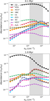 |
Fig. 2 Chemical models computed with NAUTILUS for 0.1 Myr (top) and 1.0 Myr (bottom). The densities covered by the grids are defined so that the minimum and maximum values reached by the simulations are included. The shaded region in both plots corresponds to the density range P1.5 ≤ ρ ≤ P98.5, so most of the simulation cells (97%) are included in this interval. |
Rotational transitions considered for the line radiative transfer.
4 Kinematics: Line profiles
First, we explored the influence of the relative alignment between the line of sight (LoS) and the global magnetic field direction, which is mostly parallel to the x-axis, on the predicted line profiles. For better illustrating this situation, in Fig. 3 we show the column density maps  for the simulation on each of the three faces of the cube; two of the faces (xy, xz) are perpendicular to the magnetic field direction, while the third face (yz) shows the column density map when integrating along the direction of the mean magnetic field. On each map, there are three individual lines of sight represented by symbols: the black circle corresponds to the line of sight with the highest column density, the white triangle to the lowest one, and the grey cross is the point of the map where the column density equals the mean column density. Also included in these plots is the IRAM beam size for 13CO (1 → 0) assuming a nominal distance of 140 pc for the cloud, which is the transition chosen for the discussion of the effects of turbulence on the kinematics. We chose 13CO instead of 12CO for this discussion because our observations as well as the post-processed simulations showed evidence to be optically thick. Besides, we decided to focus this discussion on 13CO instead of on other molecules because its emission was stronger, although other transitions should present a similar behaviour.
In Fig. 4 we show the line profiles for 13CO (1 → 0) – assuming a chemical age of 1 Myr – for these three lines of sight and for two faces of the cube, one parallel and one perpendicular to the magnetic field, as predicted by RADMC-3D for the simulation (label ‘MHD’) and after convolution with the IRAM 30 m beam (label ‘IRAM’); we include in the discussion only one of the lines of sight perpendicular to the magnetic field because the results in both cases are similar. From these plots, it is evident that the relative alignment between the line of sight and the magnetic field makes a difference in the observed line profiles, and in order to quantify these effects we computed the second-order moment (M2) of the integrated intensity maps, which gives an estimate of the spectral line width. This second-order moment is computed as:
 (2)
(2)
where Tb is the temperature of the line in K, υ is the velocity in km s−1, and M1 is the first-order moment also in km s−1:
 (3)
(3)
By definition, the units of M2 are km2 s−2, but in order to provide a quantity in spectral units (km s−1), we assume that M2 represents the variance of a Gaussian distribution, and therefore the dispersion can be computed as  , and the corresponding line width (or full width at half maximum, FWHM) is
  .
.
In Table 3, we provide some statistical measurements of the line widths of 13CO (1 → 0) for the two faces of the cube shown in Fig. 4. As first appreciated from this plot, the quantities in Table 3 show that in the ‘MHD’ case the median line widths for lines of sight perpendicular to the magnetic field are two to three times larger than for the case when the line of sight is parallel to the magnetic field. However, this dependency of line width with respect to the direction of the magnetic field might be lost when observing with a telescope due to its lower resolution. For this discussion, we assumed that our simulations correspond to a cloud located at a distance of 140 pc, providing a spatial resolution of 0.28″; on the other hand, the IRAM 30 m beam for the transition 13CO (1 → 0) is 22.32″, and we used this value to degrade the post-processed maps to the IRAM 30 m resolution. If we compare the median4 line widths for the MHD and IRAM cases, we see that for the line of sight perpendicular to the magnetic field, the IRAM line width is 1.21 times wider than in the MHD case, while for line of sight parallel to the magnetic field the difference between MHD and IRAM line widths is 2.41. This is natural, since lines of sight parallel to the magnetic field result in narrow, single line profiles for the MHD case that suffer more from convolution, while perpendicular lines of sight show a large number of discrete components, and hence a wider line width; as a consequence, convolution of lines of sight perpendicular to the magnetic field results in a lower loss of information. This difference in line structure depending on the simulation parameters is also reflected in the position velocity diagrams, provided in Appendix B.
In view of these results, it is tempting to try to establish some criterion to determine relative alignment with respect to the magnetic field based on the observed line profiles. However, we want to note that although promising, we cannot draw firm conclusions since we made many assumptions that limit our conclusions; a further discussion on the limitations of this work is provider later in the paper. Nevertheless, we want to remark that this line of research seems promising and we will properly address it in the future.
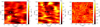 |
Fig. 3 Molecular hydrogen column density maps for the three faces of the simulation before convolution. Depending on the plane chosen the value range varies slightly, being the yz plane the one with the less appreciable differences. In the first panel, a hatched white circle represents the IRAM 30 m beam efficiency for 13CO (1 → 0), which is the molecule used for the discussion of the kinematics. On each plot, the black circle represents the line of sight with the higher column density, the white triangle the one with lower column density, and the grey cross indicates the position where the column density is equal to the mean value (3.97 × 1021 cm−2), which corresponds to a line of sight with a mean particle density of |

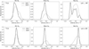 |
Fig. 4 Line profiles predicted by RADMC-3D for 13CO (1 → 0) for two faces of the cube and three lines of sight. The solid black line corresponds to the post-processed simulation, which assuming a nominal distance of d = 140 pc corresponds to a scale of 0.28″ per cell; the dashed grey line corresponds to the line profile convolved to the IRAM 30 m resolution for the selected transition, which is 22.32″. The difference in velocity range for both the upper and lower panels, which corresponds to lines of sight perpendicular (xy plane, left panel in Fig. 3) and parallel to the magnetic field (yz plane, right panel in Fig. 3) respectively. |
Statistical measurements of the line widths for13 CO (1 → 0) based on the second-order moment map.
5 Chemical abundances
The main goal of this article is to determine to what extent turbulence alone can produce significant variations on the chemistry that might explain the difficulties when fitting observations of different molecules to a single 0D chemical model. For that purpose, we post-processed our simulations as explained in Sect. 3 under the assumption that the medium is uniform (label ‘UNIF’) and post-processing the simulation with the chemical networks for 0.1 Myr, similar to the time needed to reach the stationary turbulent state, and 1.0 Myr (label ‘TURB’). In Sect. 7, we will discuss the limitations and possible uncertainties of this approach. In practice, observations are fitted assuming a single hydrogen density that may allow to retrieve a single chemical abundance, so our ‘UNIF’ case corresponds to the procedure applied in our previous observational works (GEMS I; GEMS II; GEMS IV; Bulut et al. 2021; Spezzano et al. 2022; Esplugues et al. 2022; GEMS VII).
We worked with the integrated intensity maps built from the RADMC-3D spectral cubes for each case, which will be denoted as IUNIF and ITURB; the details of how these maps are obtained for each transition can be found in Appendix C. In Fig. 5, we show the box plot for the ratio of turbulent to uniform integrated intensity maps for the case of the magnetic field perpendicular to the line of sight. We show each molecule and transition listed in Table 2 and for the two chemical ages considered, 0.1 Myr (white boxes) and 1.0 Myr (filled boxes). In this plot, each box extends from quartile Q1 (25%) to quartile Q3 (75%), and the horizontal line inside the box is the median value; the whiskers extend up to 1.5 the interquartile range (IQR, Q3–Q1), and flier points have been excluded from the plot in order to help the visualisation.
There are many conclusions that can be drawn by inspection of Fig. 5. First, as we anticipated in the view of the predicted NAUTILUS abundances for the density range and local properties considered in this work (Fig. 2), the predicted line intensities for 13CO (1 → 0) depend strongly on the chemical age. While for models with 0.1 Myr the integrated intensities computed from the simulations are slightly lower than those predicted under the uniform assumption, turbulence can only induce a slight dispersion on the integrated intensity map that is very close to the uniform value. However, at 1.0 Myr the predicted integrated intensities under the uniform assumption are a factor of ~2 lower than those predicted for the turbulent case (note the extension of the black filled box). It is known that the CO abundance is very sensitive to the chemical age in regions where the dust temperature is below 15 K (Bulut et al. 2021). This means that as long as the density is known, the CO abundance is a good chemical clock. Our results show that turbulence has a strong impact on the mean CO abundance and therefore, on the observed line intensities. To ignore the fluctuations that turbulence produces on the CO abundance would lead to an overestimation of the chemical age in dark clouds.
A similar striking behaviour is shown at 0.1 Myr for two SO (2, 3 → 1, 2) and o-H2S (110 → 101). As shown in Fig. 2, the abundance of these sulfur-bearing species are very sensitive to density, increasing by more than one order of magnitude. This translates into integrated line intensities a factor of approximately 1.5 larger in the turbulent than in the uniform case. These two species have been widely observed, especially in warm regions (Crockett et al. 2014;Esplugues etal. 2013;el Akel et al. 2022) and in bipolar outflows (Holdship et al. 2019; Schutzer et al. 2022). Also abundant in dark clouds, chemical models usually failed to reproduce their abundances in these dense and cold regions (see e.g. GEMS II). Our results show that turbulence has a large impact on their chemical abundances, especially at chemical ages of a few 0.1 Myr which best reproduce the observations of less evolved starless cores (Spezzano et al. 2022; Esplugues et al. 2022; Hily-Blant et al. 2022). We recall that our model is isothermal, thus neglecting any heating of the gas due to turbulence dissipation. The differences observed in the SO (2, 3 → 1, 2) and o-H2S (110 → 101) line intensities are only due to the variations of the density and kinematical structure in a turbulent filament.
The rest of the molecular species do not present significant variations when comparing the turbulent and uniform cases, but it is worth noting some minor dependencies. On the one hand, the integrated intensities for H13CO+ (1 → 0) are roughly similar to the uniform case for 0.1 Myr, but when fitting with a 1.0 Myr model integrated intensities for the turbulent case are larger by a factor of ~1.2. On the other hand, transitions such as H13CN (1 → 0), HNC (1 → 0), CS (2 → 1), and HCS+ (2 → 1) do not present strong dependencies on the chemical age, and the trend of the medians is similar, what may indicate that a simultaneous fitting of these four molecules to the same chemical model should produce compatible results, although if we assume again a uniform hydrogen density and molecular abundance the integrated line intensities will be overestimated by a factor of ~10–20%.
Up to this point, the discussion on the effects of turbulence on the chemistry has been mainly qualitative based on the results displayed in Fig. 5. However, in Table 4 we provide medians and interquartile ranges for all the analysed transitions and the two chemical ages considered, as well as for the post-processed simulation (MHD) and the convolved maps (IRAM), for the line of sight perpendicular and parallel to the magnetic field direction. As already discussed from the plot, most of the integrated intensities are a factor of ~10% larger when assuming a uniform gas distribution along the line of sight, with median values of the ITURB/IUNIF ratio around 0.9. However, the main exceptions are SO (2, 3 → 1, 2), and o-H2S (110 → 101) for the 0.1 Myr model, and 13CO (1 → 0) for the 1.0 Myr model, for which the post-processed simulations indicate that the line intensities should be between a factor of 1.5 and 2 higher than when assuming a uniform gas density, with large dispersions. One could argue that these statistical variations arising from turbulence could be diluted when observing with a telescope, but as can be seen from the comparison between the MHD and IRAM values in Table 4 the medians are equivalent; the main effect when degrading the resolution to the beam size is the decrease of the interquartile range (the dispersion) by an order of magnitude, which is quite significant but does not affect the main results: turbulent motions in the gas may introduce a significant dispersion in the chemistry that depends on chemical age and on the molecular species chosen.
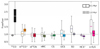 |
Fig. 5 Box plot for the ratio of integrated intensity maps ITURB /IUNIF for the case of the magnetic field perpendicular to the line of sight, where ITURB is the integrated intensity map for the full post-processed simulation and IUNIF is the intensity map assuming a constant hydrogen density (and therefore constant molecular abundance) along the line of sight. For each molecule we have two box plots: the left one corresponds to the chemical network at 0.1 Myr, and the right one at 1 Myr. The y-axis has been scaled so that the main box ranging from quartiles Q1 (25%) to Q3 (75%) is always shown and differences among all molecules can be appreciated, although in some cases the whiskers extend outside the plot. This figure corresponds to the case where the line of sight is perpendicular to the mean magnetic field direction. An analogous figure for the line of sight parallel to the magnetic field is provided in Appendix D. |
6 Comparing with single-dish observations
So far, we have focussed the discussion on the theoretical results. However, it is also important to highlight the impact that our study may have on the observations. With that purpose, we selected a subsample of the positions observed within the GEMS project in Taurus: 3 cuts in TMC-1 and 9 in B213 (GEMS IV). The cuts were selected based on their estimated temperature (around 12 K) and molecular hydrogen densities (a few 104 cm−3). As an additional constraint, we imposed a non-null detection of H13CN (1 → 0) in order to be able to do a more complete and meaningful comparison. After applying these criteria, we ended up with a sample of 37 positions with non-null detections for essentially all the transitions. The main exception is OCS (7 → 6), a transition for which we do not detect emission for 19 positions; additionally, two positions are lacking o-H2S (110 → 101) emission, and another four do not present emission of the HCS+ (2 → 1) line.
A direct comparison between our synthetic observations and real data is not easy because our simulation box represents a fraction of the cloud while observations account for emission from all the material along the line of sight. For that reason, we opted for comparing integrated line intensity ratios that are less sensitive to the length of the line of sight in the optically thin case and that are commonly used by observational astronomers (GEMS I, GEMS VII, Semenov et al. 2018; Jiménez-Donaire et al. 2019; Hacar et al. 2020; García-Rodríguez et al. 2023): 13CO (1 → 0)/H13CO+ (1 → 0), o-H2S (110 → 101)/CS (2 → 1), CS (2 → 1)/HCS+ (2 → 1), OCS (7 → 6)/SO (2, 3 → 1, 2), CS (2 → 1)/SO (2, 3 → 1, 2), 13CO (1 → 0)/H13CN (1 → 0), and H13CN (1 → 0)/HNC (1 → 0). In the case of optically thin emission, the integrated line intensity is proportional to the column density and excitation temperature of a given species in a given interval of the projected velocity along the line of sight. Therefore, it depends on the density and kinematical structure of the cloud as well as on the physical conditions of the emitting gas (i.e. its temperature). Trying to evaluate the impact of the turbulence on the chemistry, we considered: (i) the uniform case with constant density and molecular abundances explained above; and (ii) turbulent case with the densities and the chemical abundances obtained in Sect. 5. In the two cases, we used the velocity field provided when considered that the line of sight is perpendicular to the magnetic field. We are aware that some of the selected lines might be optically thick towards some positions. In order to minimise this problem we used the 13C isotopologues for HCN and HCO+. The comparison between the output of these simulations and GEMS observations is made under a descriptive approach since our observational sample is quite limited in size. For the sake of interpretation, we computed the credible regions for each simulation with a credibility level of 95% and counted the number of observational points that lay inside them, without taking into account the observational errors that arise from the line fitting process; the results are listed in Table 5. These regions are, in practice, intervals which contain the data corresponding to our synthetic populations with a probability of 95%, and are the bayesian equivalent to confidence intervals. As a complementary visual support, we computed the median and interquartile range of these synthetic distributions and the results, together with the observational measurements, are shown in Figs. 6 and 7, where we plot the predicted values for the uniform and turbulent cases coded in blue and red respectively together with the GEMS integrated intensities towards TMC-1 (circles) and B213 (triangles).
In agreement with our previous fits (GEMS VII), most of the line integrated intensity ratios are better fitted with t = 0.1 Myr. At this chemical time, the difference between the median of the 13CO/H13CO+, CS/HCS+, 13CO/H13CN, and H13CN/HNC values obtained in the uniform and turbulent cases are shallow. This is expected taking into account the results shown in Fig. 5. The differences in the integrated line intensities of these transitions between the uniform and turbulent cases are less than 50%. However, we would like to comment that this difference goes in the direction of improving the agreement between simulations and observations, indicating that our approach goes in the right direction. Moreover, this improvement is more significative if we consider the range of values (shaded red area in Figs. 6 and 7) obtained in our synthetic grid, as well as the credible regions in Table 5. For instance, all the positions in TMC-1 and a large fraction of those in B 213 lie in the shaded red area of the 13CO/H13CO+ panel, which accounts for the 54.05% of the observational data. There are three cases in which we found a large difference (larger than 50%) between the uniform and turbulent simulations. These are o-H2S/CS, OCS/SO, and CS/SO. In the case of o-H2S/CS, the inclusion of turbulence definitely improves the agreement with Taurus observations, in the sense that more observational points are contained in the credible regions for the turbulent case than for the uniform case, but in the view of the plots we do not obtain a good result yet because the median value is still quite far from the centre of the cloud of observational points. We do obtain a reasonable agreement with observations in the case of the OCS/SO ratio when considering the turbulent case at early ages (0.1 Myr). In the case of the CS/SO ratio, the dispersion in the observed values hinders to establish any conclusion, but taking turbulence into consideration increases the number of points inside the credible region from 35.14% for the uniform case up to 56.76% for the turbulent one.
Only the CS/HCS+ and o-H2S/CS ratios are better explained using t = 1 Myr. This difficulty to explain the observations of all species using the same chemical time has been previously discussed (see e.g. Bulut et al. 2021, GEMS VII and Taillard et al. 2023). Indeed, in GEMS VII we already proposed that the positions located at low extinction are better fitted with t = 1 Myr while those at higher extinctions (and densities) were fitted with shorter chemical times. Taillard et al. (2023) obtained a similar result based on methanol observations and suggested that this might be related with the dynamical evolution of the cloud contraction which is accelerated as the density increase. Regarding this interpretation, it is interesting to comment that HCS+ and H2S can be considered tracers of the most diffuse part of the gas since their emission is dominated by the outer layers of the cloud (GEMS I; GEMS II). We would also like to mention the behavior of the 13CO/H13CO+ ratio, which increases a factor of ~2 in the turbulent case compared with the uniform one. Still, the values predicted by our simulations are far from those observed in Taurus, and this is a significant difference that should be taken into account.
As a final conclusion, it is evident that, when including turbulence, model predictions approach better the observational values. The predicted median for the turbulent case always follows better the mean observational value than the uniform case, and the range it spans is always broader. This difference is especially important for the sulfur-bearing species SO, OCS, and o-H2S at early times, and for CO at ages later than a few 0.1 Myr. As a consequence, it is important to take into account turbulence when fitting the observations of these species, for instance via numerical modelling.
Statistics of relative intensity maps ITURB/IUNIF for the lines of sight considered in the discussion.
Credible regions (95%) derived from our synthetic data for the turbulent and uniform cases and percentage of observational points contained in the interval.
7 Limitations of the model
The scope of this paper was to assess if small scale structure not resolved in single-dish molecular observations could be of importance when fitting the data, and how biased the results are if a uniform medium is assumed. Therefore, we built a very simple model that responded to our needs as a first approximation, but we want to remark that there are several limitations that we disregarded for the sake of the discussion but that could be biasing our interpretation.
First of all, the numerical model presented here has not enough spatial resolution to correctly analyse the properties of the turbulence. Since we are considering quite a strong magnetic field (40 µG), Lemaster & Stone (2009) showed that for the turbulence to fully converge, we should reach a resolution of at least 5123. However, analysing the small-scale properties of the turbulence is out of the scope of this paper, and we refer the reader to the recent work by Grete et al. (2023) for a deeper discussion on that topic. In our case, we confirmed that increasing the resolution from 2563 to 5123 resulted in smoother density and velocity PDFs, but the general behaviour of the fluid is the same: the PDFs become stable after two crossing times and the differences in density distribution would be important if we were analysing the chemical evolution of the cloud at the same time as its dynamical evolution, but that is not the case. Actually, these differences in density would be lost in the step of degrading the maps at the IRAM resolution, since an IRAM beam contains ~853 cells, so we expect the comparison with observations not to be significantly biased due to the numerical resolution, although the analysis of the original MHD simulation is likely biased towards large-scale density fluctuations.
Then, we are considering separately the dynamical and chemical evolution of the cloud. In fact, we evolve our numerical model until a stage that would correspond to a physical age of 0.35 Myr, but then we post-processed this density cube with chemical models at 0.1 Myr and 1 Myr. We acknowledge that chemical stability is reached later than dynamical stability in a turbulent box (López-Dones et al., in prep.) but, on the other hand, since we are post-processing a stable density PDF with chemical models and the density in our simulations is not affected by the chemistry, it is reasonable to consider both chemical models.
Another limitation could arise from the LVG approximation for computing the molecular emission. With this approximation, we are only taking into account the density and velocity distribution of the gas, but more sophisticated methods could be followed to consider other effects apart from non-LTE (see for instance the recent work by Hegmann et al. 2006 and references therein). However, given the moderate column densities considered in this work and provided we did not observe any saturation of the lines for the chosen transitions, we assume the LVG approximation to hold for our analysis.
Finally, we want to mention that even if we are working with a limited resolution at which the turbulence is not fully resolved, we also explored other cases with different turbulent mixing modes (purely solenoidal) and magnetic field strength (90 µG) at the same resolution as the model analysed in the main core of the paper. We did not find any strong differences in the density PDFs, and the same trend of narrower line widths for lines of sight parallel to the magnetic field was observed in all cases, with increasing line widths at lines of sight perpendicular to the magnetic field as we considered stronger magnetic fields.
All in all, even if we are working with a low-resolution model we do not expect that the comparison with observations performed in Sect. 6 will be inconsistent, since we are comparing with single-dish observations. However, we aim to develop more realistic models in the future where we evolve the chemistry together with the MHD evolution at a resolution as high as possible that could serve to define new constraints when fitting observations, especially for the analysis of future interferometric data.
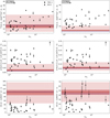 |
Fig. 6 Comparison between predicted and observed values of the ratios 13CO (1 → 0)/H13CO+ (1 → 0), o-H2S (110 → 101)/CS (2 → 1), and CS (2 → 1)/HCS+ (2 → 1). The left panels correspond to the post-processed simulations at 0.1 Myr while the right panels correspond to 1.0 Myr. On each panel, the median value for the turbulent (uniform) case is highlighted by the solid (dashed) line, the IQR is represented by the dark area and the full range (from minimum to maximum) is represented by the light-coloured area. The uniform and turbulent cases are coded in blue and red, respectively. TMC-1 points are represented by circles and B213 by triangles, and error bars are always plotted although in most cases they are smaller than the marker. The error bars correspond to the statistical errors from fitting the lines and do not include systematics (GEMS IV). |
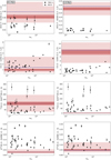 |
Fig. 7 Same as Fig. 6 but for the ratios OCS (7 → 6)/SO (2, 3 → 1, 2), CS (2 → 1)/SO (2, 3 → 1, 2), 13CO (1 → 0)/H13CN (1 → 0), and H13CN (1 → 0)/HNC (1 → 0). |
8 Conclusions
In this work, we present a study on the influence of turbulence on the chemical evolution of a molecular cloud, focussing our analysis in the density fluctuations and velocity fields induced by such turbulence. Based on a numerical MHD simulation that reproduces the steady-state of a transonic, turbulent molecular filament before collapse, we derive chemical abundances with the NAUTILUS chemistry code and retrieve synthetic maps of rotational emission for some molecules observed during the IRAM 30 m Large Programme GEMS. We explore a turbulent model with both compressive and solenoidal modes and a magnetic field strength of 40 µG, as well as two chemical ages (0.1 Myr and 1.0 Myr), and we analyse the synthetic emission maps based on the relative alignment between the observer and the mean magnetic field direction. Our main results can be summarised as follows:
When the 3D cubes of densities, velocities and abundances are post-processed with RADMC-3D for obtaining synthetic molecular line emission maps, even after convolution with the IRAM 30 m beam we observe that the line profiles for lines of sight perpendicular to the magnetic field are wider than in the case when it is parallel;
In our analysis, we computed the chemical abundances using NAUTILUS under two assumptions: that the medium is homogeneous in density along the line of sight, and that the density distribution is turbulent as given by the simulations. When turbulence is taken into account, the predicted integrated intensities are different from those derived assuming a uniform gas density along the line of sight. The differences are critical for some sulfur-bearing molecules (SO, H2S) at early ages and 13CO at 1.0 Myr (Fig. 5);
When comparing our predictions with real observations of Taurus, we find that the inclusion of turbulence always improves the results, and most of the analysed molecular ratios are compatible with the model at 0.1 Myr, the observationally derived chemical age (GEMS VII).
We conclude that turbulence may induce density variations which play an important role in shaping the chemistry of molecular clouds, especially for those molecules sensitive to hydrogen density - mainly CO and some sulfur-bearing species in the cases analysed here. Therefore, turbulence should be taken into account when trying to derive chemical abundances from observations, using for instance numerical simulations as the ones performed here with parameters relevant to those of the particular cloud under study. Other effects, such as introducing a pre-phase model or considering mixed dust populations of silicate and graphite grains might be relevant and will be explored in future works.
Acknowledgements
We want to thank the referee for their comments that helped to improve the clarity of this paper. L.B.-A. acknowledges the receipt of a Margarita Salas postdoctoral fellowship from Universidad Complutense de Madrid (CT31/21), funded by “Ministerio de Universidades” with Next Generation EU funds. L.B.-A. also wants to thank Chang-Goo Kim for useful discussions on the general use of Athena++. A.F. thanks the Spanish MICIN for funding support through grant PID2019-106235GB-I00 and the European Research Council (ERC) for funding under the Advanced Grant project SUL4LIFE, grant agreement No 101096293. R.L.G. would like to thank the "Physique Chimie du Milieu Interstellaire" (PCMI) programs of CNRS/INSU for their financial supports. A.I.G.C. and L.B.-A. acknowledge financial support through grant MINECO - PID2020-116726RB-I00. This research has made use of the computational facilities of the Joint Center for Ultraviolet Astronomy in the campus of the Universidad Complutense de Madrid, managed by J.C. Vallejo and R. de la Fuente Marcos. D.N.-A. acknowledges funding support from Fun-dación Ramón Areces through their international postdoc grant program. J.E.P. is supported by the Max-Planck Society. RMD has received funding from “la Caixa” Foundation, under agreement LCF/BQ/PI22/11910030.
Appendix A Influence of the initial conditions on the chemistry
In this work, we take all of the chemical species to be initially in atomic phase, except for hydrogen that is all locked into H2. These conditions are usually considered valid when analysing the chemical abundances in molecular clouds (see e.g. Vidal & Wakelam 2018; Wakelam et al. 2021; Agúndez et al. 2023), but we also considered the possibility of starting from a more complex medium as in Cazaux et al. (2022). With that purpose, we run a pre-phase model starting from the same abundances listed in Table 1, assuming a hydrogen density of nH = 2 × 10³ and the rest of the initial conditions as in the model detailed in Sect. 3. We follow the evolution of this lower-density medium until 1 Myr, a stage where we have many molecules formed, and take these abundances as the initial conditions for our test case. As a reference, we list in Table A.1 the 10 most abundant molecules and the main sulfur reservoirs of this prephase model, and the full list of 911 species is available as supplementary material.
Initial elemental abundances with respect to H for the 10 most abundant species of the pre-phase model plus the main sulfur reservoirs.
We considered the same density grid as in our model, with 20 density values logarithmically spaced between nH = 102 cm−3 and nH = 3.084 × 105 cm−3, and compared the predicted abundances of the model used in the article, which we will refer to as the ‘atomic’ model, with those predicted by the pre-phase model for ages ranging from 0.1 Myr to 10 Myr; the different predictions from these models for two illustrative cases, CO and CS, are shown in Fig. A.1. It is evident for the plots that the predicted abundances of both models for CO are quite similar, but there might be significant differences for the abundances of sulfur-bearing molecules such as CS at early ages. In order to quantify the possible effects of these differences in abundances between models in the predictions made in this work, we take the density values ranging from the 1.5% and 98.5% percentiles of our PDF (shaded region in Fig. 2) and analysed the time evolution of the ratio of abundances for our molecules of interest; these predictions are shown in Fig. A.2.
As can be seen in Fig. A.2, the predictions of both models at an age of 1 Myr are almost equivalent, and differences can arise for chemical ages between 0.1 Myr and 1 Myr; in the remaining of this section, we will mainly discuss the differences at 0.1 Myr and 1 Myr, which are the chemical ages analysed in this work, but it is important to note that the peak of the ratio is usually reached at ages around 0.3 Myr.
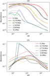 |
Fig. A.1 Predicted abundances for CO (top) and CS (bottom) of the pre-phase model (solid lines) and the atomic model (dashed lines) over the density grid considered in this work. Different chemical ages are colour-coded as shown in the legend. |
As we have already mentioned, the differences between models at 1 Myr are barely appreciable, but at early ages (0.1 Myr) the predictions might deviate up to a factor of two, especially when sulfur-bearing molecules are concerned. As an illustrative case, we analysed the differences that might arise for CS, which is one of the molecules mostly affected by the initial conditions at 0.1 Myr. If we start from a medium where all the C is in C+ (atomic model), at 0.1 Myr the predicted abundances might be twice larger than those given by the pre-phase model, especially at lower densities (see Fig. A.1). In order to assess the extent of the influence of these abundance variations in the integrated intensities, we built a molecular line emission map for CS (2 → 1) with the pre-phase model and the line of sight perpendicular to the magnetic field, and compared the integrated line intensities with those of the atomic model. We observed that the integrated line intensities for the atomic model are ~1.1–1.3 times larger than those given by the pre-phase model. However, if we compare the intensity ratios for the pre-phase model between the turbulent and uniform models, we obtain a mean value of ITURB/IUNIF = 0.95 with an interquartile range of 0.12, which is compatible with the results shown in Fig. 5. In consequence, although the chemistry at early ages is influenced by the initial conditions, especially for sulfur-bearing molecules, the results derived in this paper are self-consistent and not affected by the chemical initial conditions, even at early ages (0.1 Myr).
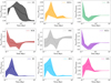 |
Fig. A.2 Time evolution of the ratio between the abundances predicted by the model that considers initial atomic abundances (main paper) and the abundances as given by the pre-phase model (this section). The solid line represents the mean ratio, while the shaded area delimits the interquartile range. For generating these plots, we only considered density values between percentiles 1.5% and 98.5% of the density PDF analysed in the main core of the paper, which roughly corresponds to nH = 1.40 × 104 cm−3 and nH = 1.20 × 105 cm−3. |
Appendix B Position Velocity diagrams
In this section, supplementary material for the discussion on the effects of turbulence on the kinematics (Sect. 4) is provided in the form of Position Velocity (PV) diagrams. In Fig. B.1 we show several PV diagrams for the two lines of sight discussed in 4, one perpendicular and one parallel to the magnetic field (left and right panels in Fig. 3); we decided to also show two different vertical cuts ofeach image to highlightthe variability ofthe velocity structures. Cuts corresponding to the same line of sight show a similar behaviour: structures in the lines of sight perpendicular to the magnetic field are more extended, while those with a parallel alignment have less velocity dispersion, resulting in a single filament-like morphology.
Appendix C Line radiative transfer of molecules with low excitation temperatures
As explained in the RADMC-3D manual, the line-integrated mean intensity for the LVG + EscProb method is given by:
 (C.1)
(C.1)
where  is the contribution of the background radiation field to the intensity of the line, which by default is set to correspond to a blackbody at 2.73 K. Therefore, any line profiles predicted with this method will include the mean intensity of this background. In observational works, the background is usually removed via the on-off technique, that is, observing the source and a nearby position without emission - the background, or via frequency switching. For radiative transitions with high excitation temperatures such as13 CO (1 → 0) the contribution of the background to the total intensity of the line will be very small – it is roughly 0.0005%. However, some rotational transitions considered in this study have low excitation temperatures very similar to the background temperature, and for those cases the contribution will affect considerably the total integrated intensity; that is the case for H13CN (1 → 0) and, to a lower extent, H13CO+. The question is, then, how can we remove this background emission. In the view of equation C.1, it is clear that we can recover the radiative emission from the background making the source function:
 (C.2)
(C.2)
where ni is the density fraction of the molecule in level i and Ai,j, Bj,i, and Bi,j are the usual Einstein coefficients. We can impose Si,j ∼ 0 forcing the full molecular fraction to be at the lowest energy level, that is, supressing the collisional excitation. Therefore, we run a set of simulations for H13CN and H13CO+ where we set the hydrogen densities to values very near to 0 (actually  to avoid numerical errors). In Fig. C.1 we show the differences that might arise between the line profile of H13CO+ (1 → 0) as given by RADMC-3D, with the background emission, and when we substract this background. For our analysis of H13CN (1 → 0) and H13CO+ (1 → 0), we used these substracted profiles.
 |
Fig. B.1 Position Velocity diagrams for the line of sight perpendicular to the magnetic field direction (columns 1 and 2) and parallel (columns 3 and 4) in two slices of the cube. The contours have been drawn at 0.4Tmax, 0.6Tmax and 0.8Tmax, where Tmax is the maximum intensity on each map. |
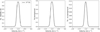 |
Fig. C.1 Comparison between line profiles. Left: line profile for H13CN (1 → 0) as given by RADMC-3D. Middle: line profile for the same setup than left panel, but setting the hydrogen density near to zero, and therefore corresponding to the background contribution. Right: resulting line profile when we substract the background (middle plot) to the RADMC-3D profile (left plot). Line profiles like the one on the right are those that we used for the analysis of H13CN (1 → 0) and H13CO+ (1 → 0). |
Appendix D Additional figure
In this appendix, we present the complementary plot to Fig. 5, that is, the box plot for the ratio of integrated intensity maps for the case of the magnetic field parallel to the line of sight (Fig. D.1).
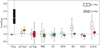 |
Fig. D.1 Box plot for the ratio of integrated intensity maps ITURB/IUNIF for the case of the magnetic field parallel to the line of sight, where ITURB is the integrated intensity map for the full post-processed simulation and IUNIF is the intensity map assuming a constant hydrogen density (and therefore constant molecular abundance) along the line of sight. For each molecule we have two box plots: the left one corresponds to the chemical network at 0.1 Myr, and the right one at 1 Myr. The y-axis has been scaled so that the main box ranging from quartiles Q1 (25%) to Q3 (75%) is always shown and differences among all molecules can be appreciated, although in some cases the whiskers extend outside the plot. |
References
- Agúndez, M., Loison, J. C., Hickson, K. M., et al. 2023, A&A, 673, A34 [NASA ADS] [CrossRef] [EDP Sciences] [Google Scholar]
- Beitia-Antero, L., Gómez de Castro, A. I., & Vallejo, J. C. 2021, ApJ, 908, 112 [NASA ADS] [CrossRef] [Google Scholar]
- Bialy, S., Burkhart, B., & Sternberg, A. 2017, ApJ, 843, 92 [NASA ADS] [CrossRef] [Google Scholar]
- Bialy, S., Neufeld, D., Wolfire, M., Sternberg, A., & Burkhart, B. 2019, ApJ, 885, 109 [NASA ADS] [CrossRef] [Google Scholar]
- Bisbas, T. G., Tanaka, K. E. I., Tan, J. C., Wu, B., & Nakamura, F. 2017, ApJ, 850, 23 [NASA ADS] [CrossRef] [Google Scholar]
- Bulut, N., Roncero, O., Aguado, A., et al. 2021, A&A, 646, A5 [NASA ADS] [CrossRef] [EDP Sciences] [Google Scholar]
- Cazaux, S., Carrascosa, H., Muñoz Caro, G. M., et al. 2022, A&A, 657, A100 [NASA ADS] [CrossRef] [EDP Sciences] [Google Scholar]
- Chapman, N. L., Goldsmith, P. F., Pineda, J. L., et al. 2011, ApJ, 741, 21 [NASA ADS] [CrossRef] [Google Scholar]
- Coutens, A., Commerçon, B., & Wakelam, V. 2020, A&A, 643, A108 [EDP Sciences] [Google Scholar]
- Crane, P., Lambert, D. L., & Sheffer, Y. 1995, ApJS, 99, 107 [NASA ADS] [CrossRef] [Google Scholar]
- Crockett, N. R., Bergin, E. A., Neill, J. L., et al. 2014, ApJ, 781, 114 [NASA ADS] [CrossRef] [Google Scholar]
- Dagdigian, P. J. 2020, MNRAS, 494, 5239 [NASA ADS] [CrossRef] [Google Scholar]
- Dobashi, K., Shimoikura, T., Nakamura, F., et al. 2018, ApJ, 864, 82 [NASA ADS] [CrossRef] [Google Scholar]
- Dullemond, C. P., Juhasz, A., Pohl, A., et al. 2012, RADMC-3D: A multipurpose radiative transfer tool, Astrophysics Source Code Library [record ascl:1202.015] [Google Scholar]
- Dumouchel, F., Klos, J., & Lique, F. 2011, Phys. Chem. Chem. Phys. (Incorp. Faraday Trans.), 13, 8204 [NASA ADS] [CrossRef] [Google Scholar]
- el Akel, M., Kristensen, L. E., Le Gal, R., et al. 2022, A&A, 659, A100 [CrossRef] [EDP Sciences] [Google Scholar]
- Esplugues, G. B., Tercero, B., Cernicharo, J., et al. 2013, A&A, 556, A143 [NASA ADS] [CrossRef] [EDP Sciences] [Google Scholar]
- Esplugues, G., Fuente, A., Navarro-Almaida, D., et al. 2022, A&A, 662, A52 [NASA ADS] [CrossRef] [EDP Sciences] [Google Scholar]
- Federrath, C. 2013, MNRAS, 436, 1245 [NASA ADS] [CrossRef] [Google Scholar]
- Federrath, C., Roman-Duval, J., Klessen, R. S., Schmidt, W., & Mac Low, M. M. 2010, A&A, 512, A81 [NASA ADS] [CrossRef] [EDP Sciences] [Google Scholar]
- Ferrada-Chamorro, S., Lupi, A., & Bovino, S. 2021, MNRAS, 505, 3442 [NASA ADS] [CrossRef] [Google Scholar]
- Flower, D. R. 1999, MNRAS, 305, 651 [Google Scholar]
- Franeck, A., Walch, S., Seifried, D., et al. 2018, MNRAS, 481, 4277 [NASA ADS] [CrossRef] [Google Scholar]
- Friesen, R. K., Pineda, J. E., co-PIs, et al. 2017, ApJ, 843, 63 [NASA ADS] [CrossRef] [Google Scholar]
- Fuente, A., Navarro, D. G., Caselli, P., et al. 2019, A&A, 624, A105 [NASA ADS] [CrossRef] [EDP Sciences] [Google Scholar]
- Fuente, A., Rivière-Marichalar, P., Beitia-Antero, L., et al. 2023, A&A, 670, A114 [NASA ADS] [CrossRef] [EDP Sciences] [Google Scholar]
- García-Rodríguez, A., Usero, A., Leroy, A. K., et al. 2023, A&A, 672, A96 [NASA ADS] [CrossRef] [EDP Sciences] [Google Scholar]
- Ge, J. X., He, J. H., & Yan, H. R. 2016, MNRAS, 455, 3570 [NASA ADS] [CrossRef] [Google Scholar]
- Godard, B., Falgarone, E., & Pineau des Forêts, G. 2014, A&A, 570, A27 [NASA ADS] [CrossRef] [EDP Sciences] [Google Scholar]
- Godard, B., Pineau des Forêts, G., Hennebelle, P., Bellomi, E., & Valdivia, V. 2023, A&A, 669, A74 [NASA ADS] [CrossRef] [EDP Sciences] [Google Scholar]
- Gratier, P., Majumdar, L., Ohishi, M., et al. 2016, ApJS, 225, 25 [Google Scholar]
- Green, S., & Chapman, S. 1978, ApJS, 37, 169 [Google Scholar]
- Grete, P., O’Shea, B. W., & Beckwith, K. 2023, ApJ, 942, L34 [CrossRef] [Google Scholar]
- Hacar, A., Bosman, A. D., & van Dishoeck, E. F. 2020, A&A, 635, A4 [NASA ADS] [CrossRef] [EDP Sciences] [Google Scholar]
- Hacar, A., Clark, S. E., Heitsch, F., et al. 2023, Protostars and Planets VII, eds. S. Inutsuka, Y. Aikawa, T. Muto, K. Tomida, & M. Tamura, ASP Conf. Ser., 534, 153 [NASA ADS] [Google Scholar]
- Hegmann, M., Hengel, C., Röllig, M., & Kegel, W. H. 2006, A&A, 445, 591 [NASA ADS] [CrossRef] [EDP Sciences] [Google Scholar]
- Hennebelle, P., & Falgarone, E. 2012, A&A Rev., 20, 55 [NASA ADS] [CrossRef] [Google Scholar]
- Heyer, M. H., & Brunt, C. M. 2004, ApJ, 615, L45 [NASA ADS] [CrossRef] [Google Scholar]
- Hily-Blant, P., Pineau des Forêts, G., Faure, A., & Lique, F. 2022, A&A, 658, A168 [NASA ADS] [CrossRef] [EDP Sciences] [Google Scholar]
- Hincelin, U., Wakelam, V., Commerçon, B., Hersant, F., & Guilloteau, S. 2013, ApJ, 775, 44 [NASA ADS] [CrossRef] [Google Scholar]
- Hincelin, U., Commerçon, B., Wakelam, V., et al. 2016, ApJ, 822, 12 [NASA ADS] [CrossRef] [Google Scholar]
- Holdship, J., Jimenez-Serra, I., Viti, S., et al. 2019, ApJ, 878, 64 [NASA ADS] [CrossRef] [Google Scholar]
- Hsu, C.-J., Tan, J. C., Goodson, M. D., et al. 2021, MNRAS, 502, 1104 [Google Scholar]
- Jiménez-Donaire, M. J., Bigiel, F., Leroy, A. K., et al. 2019, ApJ, 880, 127 [CrossRef] [Google Scholar]
- Katz, H. 2022, MNRAS, 512, 348 [NASA ADS] [CrossRef] [Google Scholar]
- Koch, E. W., Ward, C. G., Offner, S., Loeppky, J. L., & Rosolowsky, E. W. 2017, MNRAS, 471, 1506 [NASA ADS] [CrossRef] [Google Scholar]
- Körtgen, B., Bovino, S., Schleicher, D. R. G., Giannetti, A., & Banerjee, R. 2017, MNRAS, 469, 2602 [Google Scholar]
- Lane, H. B., Grudic, M. Y., Guszejnov, D., et al. 2022, MNRAS, 510, 4767 [NASA ADS] [CrossRef] [Google Scholar]
- Lemaster, M. N., & Stone, J. M. 2009, ApJ, 691, 1092 [NASA ADS] [CrossRef] [Google Scholar]
- Lique, F., Spielfiedel, A., & Cernicharo, J. 2006, A&A, 451, 1125 [NASA ADS] [CrossRef] [EDP Sciences] [Google Scholar]
- Lique, F., Senent, M. L., Spielfiedel, A., & Feautrier, N. 2007, J. Chem. Phys., 126, 164312 [NASA ADS] [CrossRef] [Google Scholar]
- Loinard, L., Torres, R. M., Mioduszewski, A. J., et al. 2007, ApJ, 671, 546 [NASA ADS] [CrossRef] [Google Scholar]
- Lucas, R., & Liszt, H. 1996, A&A, 307, 237 [NASA ADS] [Google Scholar]
- Lynn, J. W., Parrish, I. J., Quataert, E., & Chandran, B. D. G. 2012, ApJ, 758, 78 [NASA ADS] [CrossRef] [Google Scholar]
- Messinger, D. W., Whittet, D. C. B., & Roberge, W. G. 1997, ApJ, 487, 314 [NASA ADS] [CrossRef] [Google Scholar]
- Moseley, E. R., Draine, B. T., Tomida, K., & Stone, J. M. 2021, MNRAS, 500, 3290 [Google Scholar]
- Myers, A. T., McKee, C. F., & Li, P. S. 2015, MNRAS, 453, 2747 [Google Scholar]
- Navarro-Almaida, D., Le Gal, R., Fuente, A., et al. 2020, A&A, 637, A39 [NASA ADS] [CrossRef] [EDP Sciences] [Google Scholar]
- Navarro-Almaida, D., Bop, C. T., Lique, F., et al. 2023, A&A, 670, A110 [NASA ADS] [CrossRef] [EDP Sciences] [Google Scholar]
- Navarro-Almaida, D., Lebreuilly, U., Hennebelle, P., et al. 2024, A&A, 685, A112 [NASA ADS] [CrossRef] [EDP Sciences] [Google Scholar]
- Neufeld, D. A., Falgarone, E., Gerin, M., et al. 2012, A&A, 542, L6 [NASA ADS] [CrossRef] [EDP Sciences] [Google Scholar]
- Onus, A., Krumholz, M. R., & Federrath, C. 2018, MNRAS, 479, 1702 [NASA ADS] [CrossRef] [Google Scholar]
- Rodríguez-Baras, M., Fuente, A., Riviére-Marichalar, P., et al. 2021, A&A, 648, A120 [NASA ADS] [CrossRef] [EDP Sciences] [Google Scholar]
- Ruaud, M., Wakelam, V., & Hersant, F. 2016, MNRAS, 459, 3756 [Google Scholar]
- Savage, C., Apponi, A. J., Ziurys, L. M., & Wyckoff, S. 2002, ApJ, 578, 211 [NASA ADS] [CrossRef] [Google Scholar]
- Schutzer, A. de A., Rivera-Ortiz, P. R., Lefloch, B., et al. 2022, A&A, 662, A104 [NASA ADS] [CrossRef] [EDP Sciences] [Google Scholar]
- Seifried, D., & Walch, S. 2016, MNRAS, 459, L11 [NASA ADS] [CrossRef] [Google Scholar]
- Seifried, D., Sánchez-Monge, Á., Suri, S., & Walch, S. 2017a, MNRAS, 467, 4467 [NASA ADS] [CrossRef] [Google Scholar]
- Seifried, D., Walch, S., Girichidis, P., et al. 2017b, MNRAS, 472, 4797 [NASA ADS] [CrossRef] [Google Scholar]
- Semenov, D., Favre, C., Fedele, D., et al. 2018, A&A, 617, A28 [NASA ADS] [CrossRef] [EDP Sciences] [Google Scholar]
- Shetty, R., Glover, S. C., Dullemond, C. P., & Klessen, R. S. 2011, MNRAS, 412, 1686 [NASA ADS] [CrossRef] [Google Scholar]
- Sipilä, O., Caselli, P., Redaelli, E., & Spezzano, S. 2022, A&A, 668, A131 [NASA ADS] [CrossRef] [EDP Sciences] [Google Scholar]
- Spezzano, S., Fuente, A., Caselli, P., et al. 2022, A&A, 657, A10 [NASA ADS] [CrossRef] [EDP Sciences] [Google Scholar]
- Stone, J. M., Tomida, K., White, C. J., & Felker, K. G. 2020, ApJS, 249, 4 [NASA ADS] [CrossRef] [Google Scholar]
- Taillard, A., Wakelam, V., Gratier, P., et al. 2023, A&A, 670, A141 [NASA ADS] [CrossRef] [EDP Sciences] [Google Scholar]
- Tokuda, K., Onishi, T., Saigo, K., et al. 2018, ApJ, 862, 8 [NASA ADS] [CrossRef] [Google Scholar]
- Tritsis, A., Panopoulou, G. V., Mouschovias, T. C., Tassis, K., & Pavlidou, V. 2015, MNRAS, 451, 4384 [NASA ADS] [CrossRef] [Google Scholar]
- van der Tak, F. F. S., Black, J. H., Schöier, F. L., Jansen, D. J., & van Dishoeck, E. F. 2007, A&A, 468, 627 [NASA ADS] [CrossRef] [EDP Sciences] [Google Scholar]
- Vidal, T. H. G., & Wakelam, V. 2018, MNRAS, 474, 5575 [Google Scholar]
- Wakelam, V., Gratier, P., Ruaud, M., et al. 2021, A&A, 647, A172 [NASA ADS] [CrossRef] [EDP Sciences] [Google Scholar]
- Weingartner, J. C., & Draine, B. T. 2001, ApJS, 134, 263 [CrossRef] [Google Scholar]
- Yang, B., Stancil, P. C., Balakrishnan, N., & Forrey, R. C. 2010, ApJ, 718, 1062 [Google Scholar]
- Yazidi, O., Ben Abdallah, D., & Lique, F. 2014, MNRAS, 441, 664 [NASA ADS] [CrossRef] [Google Scholar]
This median is computed taking into account all the image pixels, including the borders. However, the differences in the median if borders are removed are of the order of 1%.
All Tables
Statistical measurements of the line widths for13 CO (1 → 0) based on the second-order moment map.
Statistics of relative intensity maps ITURB/IUNIF for the lines of sight considered in the discussion.
Credible regions (95%) derived from our synthetic data for the turbulent and uniform cases and percentage of observational points contained in the interval.
Initial elemental abundances with respect to H for the 10 most abundant species of the pre-phase model plus the main sulfur reservoirs.
All Figures
|
Fig. 1 Density and velocity probability density functions (PDFs) at the final stage of the simulation (~0.36 Myr). |
| In the text | |
|
Fig. 2 Chemical models computed with NAUTILUS for 0.1 Myr (top) and 1.0 Myr (bottom). The densities covered by the grids are defined so that the minimum and maximum values reached by the simulations are included. The shaded region in both plots corresponds to the density range P1.5 ≤ ρ ≤ P98.5, so most of the simulation cells (97%) are included in this interval. |
| In the text | |
|
Fig. 3 Molecular hydrogen column density maps for the three faces of the simulation before convolution. Depending on the plane chosen the value range varies slightly, being the yz plane the one with the less appreciable differences. In the first panel, a hatched white circle represents the IRAM 30 m beam efficiency for 13CO (1 → 0), which is the molecule used for the discussion of the kinematics. On each plot, the black circle represents the line of sight with the higher column density, the white triangle the one with lower column density, and the grey cross indicates the position where the column density is equal to the mean value (3.97 × 1021 cm−2), which corresponds to a line of sight with a mean particle density of |
| In the text | |
|
Fig. 4 Line profiles predicted by RADMC-3D for 13CO (1 → 0) for two faces of the cube and three lines of sight. The solid black line corresponds to the post-processed simulation, which assuming a nominal distance of d = 140 pc corresponds to a scale of 0.28″ per cell; the dashed grey line corresponds to the line profile convolved to the IRAM 30 m resolution for the selected transition, which is 22.32″. The difference in velocity range for both the upper and lower panels, which corresponds to lines of sight perpendicular (xy plane, left panel in Fig. 3) and parallel to the magnetic field (yz plane, right panel in Fig. 3) respectively. |
| In the text | |
|
Fig. 5 Box plot for the ratio of integrated intensity maps ITURB /IUNIF for the case of the magnetic field perpendicular to the line of sight, where ITURB is the integrated intensity map for the full post-processed simulation and IUNIF is the intensity map assuming a constant hydrogen density (and therefore constant molecular abundance) along the line of sight. For each molecule we have two box plots: the left one corresponds to the chemical network at 0.1 Myr, and the right one at 1 Myr. The y-axis has been scaled so that the main box ranging from quartiles Q1 (25%) to Q3 (75%) is always shown and differences among all molecules can be appreciated, although in some cases the whiskers extend outside the plot. This figure corresponds to the case where the line of sight is perpendicular to the mean magnetic field direction. An analogous figure for the line of sight parallel to the magnetic field is provided in Appendix D. |
| In the text | |
|
Fig. 6 Comparison between predicted and observed values of the ratios 13CO (1 → 0)/H13CO+ (1 → 0), o-H2S (110 → 101)/CS (2 → 1), and CS (2 → 1)/HCS+ (2 → 1). The left panels correspond to the post-processed simulations at 0.1 Myr while the right panels correspond to 1.0 Myr. On each panel, the median value for the turbulent (uniform) case is highlighted by the solid (dashed) line, the IQR is represented by the dark area and the full range (from minimum to maximum) is represented by the light-coloured area. The uniform and turbulent cases are coded in blue and red, respectively. TMC-1 points are represented by circles and B213 by triangles, and error bars are always plotted although in most cases they are smaller than the marker. The error bars correspond to the statistical errors from fitting the lines and do not include systematics (GEMS IV). |
| In the text | |
|
Fig. 7 Same as Fig. 6 but for the ratios OCS (7 → 6)/SO (2, 3 → 1, 2), CS (2 → 1)/SO (2, 3 → 1, 2), 13CO (1 → 0)/H13CN (1 → 0), and H13CN (1 → 0)/HNC (1 → 0). |
| In the text | |
|
Fig. A.1 Predicted abundances for CO (top) and CS (bottom) of the pre-phase model (solid lines) and the atomic model (dashed lines) over the density grid considered in this work. Different chemical ages are colour-coded as shown in the legend. |
| In the text | |
|
Fig. A.2 Time evolution of the ratio between the abundances predicted by the model that considers initial atomic abundances (main paper) and the abundances as given by the pre-phase model (this section). The solid line represents the mean ratio, while the shaded area delimits the interquartile range. For generating these plots, we only considered density values between percentiles 1.5% and 98.5% of the density PDF analysed in the main core of the paper, which roughly corresponds to nH = 1.40 × 104 cm−3 and nH = 1.20 × 105 cm−3. |
| In the text | |
|
Fig. B.1 Position Velocity diagrams for the line of sight perpendicular to the magnetic field direction (columns 1 and 2) and parallel (columns 3 and 4) in two slices of the cube. The contours have been drawn at 0.4Tmax, 0.6Tmax and 0.8Tmax, where Tmax is the maximum intensity on each map. |
| In the text | |
|
Fig. C.1 Comparison between line profiles. Left: line profile for H13CN (1 → 0) as given by RADMC-3D. Middle: line profile for the same setup than left panel, but setting the hydrogen density near to zero, and therefore corresponding to the background contribution. Right: resulting line profile when we substract the background (middle plot) to the RADMC-3D profile (left plot). Line profiles like the one on the right are those that we used for the analysis of H13CN (1 → 0) and H13CO+ (1 → 0). |
| In the text | |
|
Fig. D.1 Box plot for the ratio of integrated intensity maps ITURB/IUNIF for the case of the magnetic field parallel to the line of sight, where ITURB is the integrated intensity map for the full post-processed simulation and IUNIF is the intensity map assuming a constant hydrogen density (and therefore constant molecular abundance) along the line of sight. For each molecule we have two box plots: the left one corresponds to the chemical network at 0.1 Myr, and the right one at 1 Myr. The y-axis has been scaled so that the main box ranging from quartiles Q1 (25%) to Q3 (75%) is always shown and differences among all molecules can be appreciated, although in some cases the whiskers extend outside the plot. |
| In the text | |
Current usage metrics show cumulative count of Article Views (full-text article views including HTML views, PDF and ePub downloads, according to the available data) and Abstracts Views on Vision4Press platform.
Data correspond to usage on the plateform after 2015. The current usage metrics is available 48-96 hours after online publication and is updated daily on week days.
Initial download of the metrics may take a while.