| Issue |
A&A
Volume 687, July 2024
|
|
|---|---|---|
| Article Number | A95 | |
| Number of page(s) | 23 | |
| Section | Stellar atmospheres | |
| DOI | https://doi.org/10.1051/0004-6361/202449403 | |
| Published online | 02 July 2024 | |
Transitions in magnetic behavior at the substellar boundary
1
Institut für Astronomie & Astrophysik, Eberhard Karls Universität Tübingen,
Sand 1,
72076
Tübingen,
Germany
e-mail: This email address is being protected from spambots. You need JavaScript enabled to view it.
2
INAF – Osservatorio Astronomico di Palermo,
Piazza del Parlamento 1,
90134
Palermo,
Italy
3
Space Telescope Science Institute,
3700 San Martin Drive,
Baltimore,
MD,
USA
4
Center for Astrophysical Sciences, Johns Hopkins University,
3701 San Martin Drive,
Baltimore,
MD,
USA
5
Laboratory for Atmospheric and Space Physics, University of Colorado Boulder,
Boulder,
CO, USA
6
Department of Astronomy, University of Washington,
Seattle,
WA,
USA
Received:
30
January
2024
Accepted:
1
April
2024
Abstract
We aim to advance our understanding of magnetic activity and the underlying dynamo mechanism at the end of the main sequence. To this end, we have embarked on collecting simultaneous X-ray and radio observations for a sample of M7..L0 dwarfs in the solar neighborhood using XMM-Newton jointly with the Jansky Very Large Array (JVLA) and the Australia Telescope Compact Array (ATCA). We supplemented the data from these dedicated campaigns with X-ray data from the all-sky surveys of the ROentgen Survey with an Imaging Telescope Array (eROSITA) on board the Russian Spektrum-Roentgen-Gamma mission (SRG). Moreover, we complement this multiwavelength data set with rotation periods that we measured from light curves acquired with the Transiting Exoplanet Survey Satellite (TESS). We limited the sample to objects with rotation period of < 1 day, focusing on the study of a transition in magnetic behavior suggested by a drastic change in the radio detection rate at υ sin i ≈ 38 km s−1, corresponding to Prot ≈ 0.2 day for a typical ultracool dwarf (UCD) radius of R★ = 0.15 R⊙. Finally, to enlarge the target list, we have compiled archival X-ray and radio data for UCDs from the literature, and we have analyzed the abovementioned ancillary eROSITA and TESS observations for these objects’ analogous to the targets from our dedicated X-ray/radio campaigns. We compiled the most up to date radio/X-ray luminosity (LR,ν − Lx) relation for 26 UCDs with rotation periods (Prot) lower than 1 day, finding that rapid rotators lie the furthest away from the “Güdel-Benz” relation previously studied for earlier-type stars. Radio bursts are mainly (although not exclusively) experienced by very fast UCDs (Prot ≤ 0.2 day), while X-ray flares are seen by objects spanning the whole range of rotation. Finally, we examined the Lx/Lbol versus Prot relation, where our sample of UCDs spans a large activity level range, that is log(Lx/Lbol) = −5.5 to log(Lx/Lbol) = −3. Although they are all fast rotating, X-ray activity evidently decouples from that of normal dynamos. In fact, we found no evident relation between the X-ray emission and rotation, reinforcing previous speculations on a bimodal dynamo across late-type dwarfs. One radio-detected object, 2MJ0838, has a rotation period consistent with the range of auroral bursting sources; while it displays moderately circularly polarized emission, there is no temporal variation in the polarized flux. A radio flare from this object is interpreted as gyrosynchrotron emission, and it displays X-ray and optical flares. Among the ten UCDs observed with the dedicated X-ray/radio campaigns, we found a slowly rotating apparent auroral emitter (2MJ0752) that is also one of the X-ray brightest radio-detected UCDs. We speculate that this UCD is experiencing a transition in its magnetic behavior since it produces signatures expected from higher-mass M dwarfs along with emerging evidence of auroral emission.
Key words: stars: activity / stars: coronae / stars: low-mass / stars: magnetic field / starspots
© The Authors 2024
 Open Access article, published by EDP Sciences, under the terms of the Creative Commons Attribution License (https://creativecommons.org/licenses/by/4.0), which permits unrestricted use, distribution, and reproduction in any medium, provided the original work is properly cited.
This article is published in open access under the Subscribe to Open model. This email address is being protected from spambots. You need JavaScript enabled to view it. to support open access publication.
1 Introduction
Stellar magnetic activity is a fundamental ingredient in defining the observed spectral flux of low-mass stars. Magnetism powers chromospheres and coronae, which exhibit emissions from X-ray to radio wavebands (see review by Linsky 2017), but it also generates variability through, for example, photospheric spots, active regions, and flaring reconnection events (see Solanki et al. 2006). Observations of these emissions serve as critical diagnostics of the dynamic plasma of the stellar atmosphere, and they must be physically linked with the internally generated magnetic dynamo (e.g., Browning 2008). This connection is well evinced by multiwavelength results demonstrating rotation-activity-age correlations (e.g., Wright et al. 2018; Newton et al. 2017; Magaudda et al. 2020; Pineda et al. 2021), tying the activity to long-term angular momentum evolution. Despite a concerted effort studying stellar activity, many aspects of the underlying physics remain uncertain (e.g., dynamo mechanism, winds, coronal heating, etc.), especially in low-mass stars which often show stronger magnetic fields (e.g., Shulyak et al. 2017) and more energetic eruptions (e.g., Günther et al. 2020) relative to what has been observed from the Sun.
Understanding these effects of the stellar magnetic field are more important now than ever before because of the proliferation of detected exoplanetary systems around low-mass stars. These stars host many of the extrasolar planets most favorable for atmospheric characterization (e.g., Morley et al. 2017), and interpreting those results requires understanding the high-energy stellar emissions and their evolutionary history (e.g., Johnstone et al. 2021). Of particular interest are very low-mass stars at the end of the main sequence, which are capable of hosting multiple temperate Earth-sized planets (e.g., TRAPPIST-1; Gillon et al. 2017), and they can display enhanced magnetic activity for several billions of years (e.g., West et al. 2008).
However, relative to warmer stars, the nature of the stellar activity must change in this mass range, and toward lower-mass brown dwarfs, as effective temperatures cool and the atmospheres become more neutral, decoupling the atmospheric dynamics from the magnetic field (e.g., Mohanty & Basri 2003; Rodríguez-Barrera et al. 2015). This regime of ultracool dwarfs (UCDs; spectral types ≥M7) displays clear deviations from the standard coronal paradigm defined by solar activity (see Pineda et al. 2017), best demonstrated by their remarkable radio emissions.
For a wide range of stars (main sequence flare stars, RS CVn binaries, weak-line T Tauri stars, and Algol binaries) there is a tight relation between the luminosity in the radio and in X-rays, underlining the close connection between nonthermal gyrosyn-chrotron radio emission and thermal X-rays (Gudel et al. 1993; Güdel & Benz 1993). This Güdel-Benz relation (hereafter GB relation), however, breaks down in the UCD regime. Several UCDs with sensitive X-ray and radio measurements are over-luminous in the radio with respect to the GB relation by factors of >1000 (e.g., Williams et al. 2014; Pineda et al. 2017). Superimposed on this quiescent, quasi-steady (synchrotron) emission, tracing radiation belt structures (Kao et al. 2023; Climent et al. 2023), are highly circularly polarized periodically pulsed bursts (e.g., Burgasser & Putman 2005; Hallinan et al. 2006, 2008; Route & Wolszczan 2012; Williams et al. 2015; Kao et al. 2016; Vedantham et al. 2020; Rose et al. 2023). This “bursting” radio component has been attributed to the electron cyclotron maser instability (ECMI; Hallinan et al. 2008), a phenomenon seen predominately in solar system giant planets that is tied to auroral electron precipitation (e.g., Zarka 2007).
Conversely, the short-term variability of typical UCDs in the X-ray band exhibits the typical signatures of flares that are likely caused by magnetic reconnection events (e.g., Stelzer et al. 2006; Berger et al. 2008; Williams et al. 2014). Long-term optical photometric monitoring of this population shows the capacity for these stars to also show white-light flares (e.g., Paudel et al. 2018; Murray et al. 2022). These behaviors suggest that much UCD magnetic activity remains analogous to that of higher-mass GKM stars.
The existing radio and X-ray data thus present a heterogeneous picture for UCDs. Indeed, the accumulation of data over the past decade have only reinforced the suggestion by Stelzer et al. (2012) of a dichotomy between radio-bursting/X-ray faint and radio-quiet/X-ray flaring UCDs, although the boundary may not be rigid. Still, the nature of the onset of this behavior near the end of the stellar main sequence is unclear. The emergence of UCD ECMI radio emission is most likely shaped by magnetic field structure and strength and the dwarf rotation rate (see Stelzer et al. 2012; Pineda et al. 2017; Pineda & Hallinan 2018).
The confirmation of resolved quiescent radio emission in the UCD LSR J1835+3259 from energetic electrons trapped in large-scale magnetic loops reinforces the idea of large-scale dipolar topologies being a critical ingredient for the radio-bright UCDs (Kao et al. 2023; Climent et al. 2023). Theoretical treatments of the engines powering the radio-bright UCDs strongly depend on the object’s rotation rate (e.g., Nichols et al. 2012; Turnpenney et al. 2017; Saur et al. 2021). Moreover, Pineda et al. (2017) used spectroscopic rotation measurements to reveal a sharp rise in the detection fraction of UCD radio emission: above υ sin i ≈ 35 km s−1 (rotation period, Prot ~ 3.5 h) the UCD detection fraction at radio wavelengths rises steeply, 4–5 times the overall rate of unbiased surveys (~10%; e.g., Lynch et al. 2016). However, the unknown inclination angle makes it difficult to ascertain the precise role of rotation in observed UCD radio emissions.
The Transiting Exoplanet Survey Satellite (TESS; Ricker et al. 2015), through its broadband optical monitoring all-sky survey enables examination of photometric rotation periods across a broad sample of stars, including nearby UCDs. With TESS, we are now in the position to put reliable constraints on all relevant parameters: rotation, X-ray and radio emission, and clearly test whether the dichotomy of UCD X-ray/radio behavior emerges strictly across the rotation period boundary suggested by Pineda et al. (2017).
In this article, we build a mini-survey of GHz radio observations and X-ray data for a carefully selected sample of UCDs accessible to TESS. Our multiwavelength analysis is designed to examine UCDs on both sides of this rotation boundary (~3.5 h), and assess the nature of their magnetically driven emissions. This sample is presented in Sect. 2, with its radio, X-ray, and optical data analysis in Sect. 3. In Sect. 4, we present interesting radio emissions for specific objects with coronal and magneto-spheric models. We finally discuss our sample across all three wavebands adopted throughout this paper (Sect. 5) and propose our conclusions in Sect. 6.
Overview of the UCDs from our X-ray/radio campaigns.
2 Sample
The focus of this work is to investigate the activity of UCDs across the boundary in terms of rotation rate, υ sin i ~ 35 km s−1, at which previous data has suggested a drastic change of the radio properties (Pineda et al. 2017). For a typical late-M dwarf this corresponds to a rotation period Prot ~ 0.15 day (≈3.5 h), justified by most radio bursters being seen equator-on. Our focus is on quantifying the multiwavelength behavior of UCDs in the areas just above and below this threshold.
To this end, we have obtained deep X-ray and radio data for ten nearby UCDs. The targets were selected with the criterion that Prot be <1 day, drawing from a larger list of UCDs for which we had preliminarily determined the rotation period from TESS light curves. Considering the decay of activity in the L dwarf regime which pushes current instruments beyond their sensitivity limits, for our campaigns we focused on UCDs with spectral types from M7 to L0. Objects with small distances were preferred to guarantee the highest achievable sensitivity for the activity measurements. The target list and the X-ray/radio instruments used for each of them is provided in Table 1. The data were obtained in three dedicated X-ray/radio campaigns carried out in 2012–2013, 2014–2015 and 2020–2021.
The X-ray observations were carried out with the X-ray Multi-Mirror mission (XMM-Newton) and the radio data were obtained from the Jansky Very Large Array (JVLA) and the Australia Telescope Compact Array (ATCA). For four UCDs X-ray and radio data were acquired simultaneous or nearly simultaneous, see Tables 2 and 3. To enlarge the data base we have searched the literature for UCDs observed in both the X-ray and the radio band, and we found 16 objects.
Our nearby targets have high proper motion, and for the match of the objects’ optical position with X-ray and radio images their apparent space motion needs to be taken into account. We, thus, have to propagate the optical positions to the X-ray/radio observing date. To this end, we first search for the Gaia counterparts (CTPs) of our targets. We started with identifying all Gaia objects in their vicinity and then narrowed down the search as described in the following. First, we matched the J2000 coordinates of our UCD sample with the coordinates given in the Gaia-DR3 catalog (epoch J2016, Gaia Collaboration 2023) within a radius of 30″. Within this radius we found 54 and 137 Gaia-DR3 CTPs for the ten UCDs from our dedicated X-ray/radio observations and the literature sample, respectively, shown in gray in Fig. 1. We then performed the proper motion1 (P.M.) correction propagating the J2016 coordinates of all these potential Gaia-DR3 CTPs backwards to the J2000 epoch. Then we calculated again the separation between the position of the UCDs in our input catalog and the position of the Gaia sources. In Fig. 1, we show how the separation between the Gaia-DR3 CTPs and the input coordinates of the UCD sample has changed after applying the P.M. correction (before and after the P.M. correction in gray and in turquoise, respectively). Each UCD has now its closest Gaia-DR3 CTP within a radius of 1″, except for one target from the literature with separation ≤6″. Given this excellent match, we adopted for each UCD this closest Gaia-DR3 CTP after the P.M. correction. We confirmed our associations checking the Gaia-DR3 source_id on Simbad2, from where we retrieved also the spectral types (SpTs).
We also made use of the All-Sky survey data of the ROentgen Survey with an Imaging Telescope Array (eROSITA, Predehl et al. 2021) on board the Russian Spektrum-Roentgen-Gamma mission (SRG, Sunyaev et al. 2021). Due to the data sharing policy our consortium eROSITA_DE has access to the western galactic half of the sky that comprises all but one of the UCDs in our sample and 7 out of 16 of the literature sample. Thus, we performed a match within 30″ between the P.M. corrected coordinates of our samples with the boresight position of the merged eRASS:4 catalog (all_s4_SourceCat3B_221031_poscorr_mpe_clean.fits) provided by the German consortium, that combines the data from all 4 eROSITA All-sky surveys. The details about how the official catalogs are compiled will be published with the first data release of eROSITA within the work by Merloni et al. (2024) on the first all-sky survey (eRASS1). Eight UCDs of our sample are detected in the eRASS:4 catalog, specifically the eRASS proved to be useful for one object, for which no observational time was allocated with XMM-Newton during our campaigns. Among the objects of the literature sample only 2 are associated with an eROSITA source listed in eRASS:4.
For both samples we derived the bolometric luminosity (Lbol) and the effective temperature (Teff) that we used to calculate the radius (R★) through the Stefan-Boltzmann law. First, we computed Tef and the bolometric correction in the J band (BCJ, J band magnitude from the Two Micron All-Sky Survey– 2MASS, Cutri et al. 2003) with the polynomial fits as a function of spectral type from Filippazzo et al. (2015). Then, we calculated the absolute J band magnitude (MJ) with the Gaia-DR3 (Gaia Collaboration 2023) distances listed in Table 4. Finally, we used the distances combined with BCJ to estimate Lbol. The uncertainties for Lbol and Tef are taken from Filippazzo et al. (2015) and they are 0.133 dex and 113 K, respectively. We computed those of the radius by performing the error propagation.
The two samples count 26 UCDs in total. Their Gaia-DR3 parameters and stellar parameters are reported in Table 4. In particular, in Col. 1 we show a reduced 2MASS name when only the epoch and the first three digits of the right ascension are displayed3. Spectral types are in Col. 2, J band magnitude and effective temperature in Cols. 3 and 4, bolometric luminosity and radii in Cols. 5 and 6. From Cols. 7 to 13, we report the Gaia-DR3 SOURCE_ID with distance, proper motion and photometry.
XMM-Newton observation log.
Observing log for radio data.
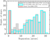 |
Fig. 1 Separation between the Gaia-DR3 (J2016) and the J2000 positions for the ten UCDs from our dedicated X-ray/radio campaigns and the 16 UCDs from the literature sample. All 191 Gaia-DR3 counterparts within 30″ are shown in gray. In turquoise there are the same objects but after the application of their P.M. correction. The red histogram represents the subsample of closest Gaia-DR3 CTPs to all UCDs after the P.M. correction. |
3 Data analysis
We describe here separately the X-ray, radio and optical photometric data analysis steps.
3.1 X-ray data analysis
3.1.1 XMM-Newton
For nine UCDs marked with ‘X’ in Table 1 we present new observations with XMM-Newton obtained during AO 11, AO 13, and AO 19 with exposure times ranging from 16 to 45 ks. We analyzed only the observations from the most sensitive instrument, the EPIC/pn imaging camera, using the XMM-Newton Science Analysis System (SAS)4 pipeline, version 20.0.0. We started the data processing with epproc which produces the EPIC/pn photon events list. We extracted the high energy light curve (LC) of the whole detector (10.0 < E < 12.0 keV) to determine the count rate above which the particle background is too high. The corresponding time intervals are removed for the further analysis. The remaining observing time forms the good time intervals (GTIs). The threshold count rate in the whole-detector light curve that defines the GTI was chosen individually for each observation based on visual inspection, and it varies from 0.4 cnt s−1 to 1.5 cnt s−1. We then filtered the event lists applying the GTIs, pixel pattern (0 ≤ pattern ≤ 12), and the #xmmea_ep filter.
We performed the source detection in five energy bands: 0.2–0.5 keV, 0.5–1.0 keV, 1.0–2.0 keV, 2.0–1.5 keV, and 4.5– 12.0 keV using SAS tools. To identify the X-ray sources associated with our sample we first propagated the Gaia-DR3 coordinates using the Gaia-DR3 proper motions to the epoch of the specific XMM-Newton observation and then we matched these expected positions of the UCDs with the X-ray coordinates from the output list of the source detection process allowing for a maximum distance of 15″. This way we establish that 6 out of 9 UCDs were detected with EPIC/pn and that their emission is mainly within 2 keV, with only few and zero counts in the 2.0–44.5 keV and 4.5–12.0 keV energy bands, respectively. The remaining three targets out of the 9 observed are undetected and they are identifiable in Table 2 where upper limits are displayed. In this table, we present all relevant X-ray parameters for the XMM-Newton observations and the results of the source detection process, namely target name (Col. 1), observation ID and date (Cols. 2 and 3), offset between the optical and X-ray coordinates (Col. 4), source counts (Col. 5), detection likelihood (Col. 6), net count rate (Col. 7), all provided by the detection algorithm for the broad energy band (0.2–12.0 keV). For the three undetected targets we calculated their upper limit count rates from the broad band sensitivity map of the EPIC/pn observations that we extracted with the SAS tool esensmap.
To enable a comparison with the literature, the energy band adopted hereafter is the combination of the softest bands we used for the source detection: 0.2–0.5 keV, 0.5–1.0 keV, and 1.0– 2.0 keV. Thus, the X-ray luminosity and the fractional X-ray luminosity, given in Cols. 8 and 9 of Table 2, refer to 0.2–2.0 keV (see Sect. 3.1.4 for the calculation of these parameters).
For the spectral and temporal analysis we retained only pixels with flag = 0. We defined a circular photon extraction region with a radius of 35″ centered on the EPIC/pn source position. The background was extracted from an adjacent source-free circular region on the same CCD chip with a radius twice that of the source region. We grouped the spectral channels such that each bin comprises a minimum of 10–20 photons depending on the brightness of the source. The response matrix and ancillary response for the spectral analysis were created using the appropriate SAS tools, rmfgen and arfgen.
As mentioned above, the X-ray emission of the detected UCDs is mainly within 2 keV, with less than 5 % of the source counts in the harder energy band of 2.0–12.0 keV. This justifies our choice of the 0.2–2.0 keV band for the extraction of the X-ray light curves. The EPIC/pn light curves for source and background were generated with the SAS tool evselect, and the background subtraction was applied using the EPICLCCORR task, which also takes care of corrections for instrumental effects such as vignetting. The corrected light curves of our sample are displayed in Fig. 2 for a 1 ks bin size and with the background emission overlaid in green. Events that are not within the GTIs, have been removed during the filtering process. This may lead to a reduced number of bins in the light curve. For instance, the light curve of LP 423-31 (see left top panel in Fig. 2) does not show any “good” event during more than half of its observation.
Visual inspection of the light curves reveals significant variability for four UCDs: 2MASS J03510004-0052 (2MJ0351), 2MASSJ17571539+7042 (2MJ1757), 2MASS J08380224-5855 (2MJ0838), and 2MASS J04351612-1606 (2MJ0435). In Fig. 2, we present the average count rate of the corrected source light curve and its standard deviation with solid and dashed blue lines, respectively. The bins located above the standard deviation upper bound can be considered to represent possible flaring activity. The four UCDs with bins that have a count rate above the standard deviation are, indeed, the same ones that we identified as variable from visual inspection.
3.1.2 eROSITA
eROSITA data was analyzed for both the UCDs from our new dedicated X-ray/radio campaigns and the literature sample defined in Sect. 2. Hereby, we made use of the preliminary version of the catalog provided by the eROSITA_DE consortium (all_s4_SourceCat3B_221031_poscorr_mpe_clean.fits) that combines the X-ray data from all 4 eROSITA All-sky surveys (eRASS:4). We propagated the Gaia-DR3 coordinates of all UCDs for their proper motion (P.M.) to the mean epoch of eRASS:4 catalog, 15 Dec 2020, and we then performed a match with the boresight corrected coordinates (RA_CORR, DEC_CORR) of eRASS:4 within 30″. We found potential eROSITA matches for 2 UCDs from the literature and 8 of the UCDs from our new X-ray/radio sample.
To confirm our association we performed a reverse match as in Magaudda et al. (2022). Starting from the eRASS:4 coordinates we looked for all possible Gaia-DR3 CTPs within 30″. We found 43 and 11 possible Gaia-DR3 CTPs for our new UCD and the literature samples, respectively. After propagating the positions of all possible Gaia CTPs to the mean eRASS:4 epoch, we selected the closest to each target of our sample we imposed that the closest eROSITA CTP must satisfy the condition that the optical and X-ray separation be smaller than three times the uncertainty of the eRASS:4 coordinates (SepX–ray,opt < 3 × RADEC_ERR). Finally, the match provided an eROSITA detection for all 8 new UCDs and 2 targets from the literature, that is all matches achieved before the reverse match were confirmed. We aim to compare the results from the analysis of XMM-Newton data to those from eROSITA in the same energy bands. Since eROSITA bands used for eRASS:4 are not the same as those of XXMM-Newton that we adopted for this work, we performed our own source detection on the eROSITA data, and we extracted the eRASS spectra and light curves for the XMM-Newton energy bands.
From the DETUID column of eRASS:4 we found in which eROSITA sky maps our targets are located. Then we downloaded the event files of the sky maps of our sample for each of the four surveys. We performed the source detection using the eSASSusers_211214 software release (Brunner et al. 2022) in the same energy bands adopted for XMM-Newton data extraction, except for the hardest band that is slightly narrower (4.5–10 keV) because eROSITA has very little effective area above 10.0 keV. After creating the exposure map, detection mask and background map within the adopted energy bands, we compiled the list of the detected sources for each of the 4 surveys using the eSASS pipeline ermldet for which we used a threshold detection maximum likelihood of 6.0. We found that 7 of the new UCDs are detected in at least one survey, that is one target less than according to the official eRASS:4 catalog. We recovered the 2 UCDs of the literature sample that are also present in eRASS:4. The missing UCD detection can be explained by different detection likelihood (DET_LIKE) thresholds. The value adopted for the compilation of the eRASS:4 catalog (DET_LIKE = 5) is smaller than ours and the missing object (2MJ0306) shows < 20 counts in eRASS:4.
With eROSITA data we added one more X-ray detection to our UCD sample that is associated to 2MASS J10551532-7356 (2MJ1055), for which no time was allocated with XMM-Newton. Moreover, we enabled a long-term variability analysis, for instance 2MASS J02150802-3040 (2MJ0215) is an upper limit with XMM-Newton but appears as a detection during the last eROSITA survey, eRASS4.
The UCDs without detection in any of the 4 eRASS all have a detection with XMM-Newton. The eRASS upper limits are shallower than the XMM-Newton data and would, therefore, not provide additional information. Therefore, we decided to ignore them and calculate the upper limits only for those targets that are detected during at least one eROSITA survey. The X-ray parameters of the eROSITA sources detected during one ormore eRASSs are given in Table 5 with the results of the upper limit calculation from the extraction of the aperture photometry with the apetool pipeline. Specifically, in Table 5 we provide the acronym for the 2MASS name of the object and the identifying number of the eROSITA survey (Cols. 1 and 2), the X-ray coordinates with their uncertainty (Cols. 3-5), the offset between the P.M. corrected optical position and the X-ray coordinates (Col. 6), the 0.2–10.0 keV count rate obtained from the source detection procedure (Col. 7), and the detection maximum likelihood in the same energy band (Col. 8). The last two columns show the Lx and Lx/Lbol values computed for the energy band of 0.2–2.0 keV, as for the XMM-Newton data (see Sect. 3.1.4).
Finally, we extracted the spectrum and light curve for each of the eROSITA detections using the srctool pipeline with the option AUTO for the choice of the source and background region sizes. The eROSITA light curves and spectra are shown in Figs. 3, A.1, and 4. None of the literature targets show a bright eROSITA detection, thus only their light curves are shown in Fig. 3. The bin size of the light curves is 14.4 ks corresponding to one eRODay, that is the time that eROSITA takes to return to the same sky position during its scanning motion (Predehl et al. 2021). This means there is one bin in the light curve for each of eROSITA’s visits of the source.
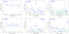 |
Fig. 2 Background-subtracted XMM-Newton EPIC/pn light curves in the energy band of 0.2–2.0 keV of the detected UCDs (blue) and the light curves of the background (green) both with a 1 ks bin size. The mean count rate and its standard deviation are shown as horizontal solid and dashed bars. |
Results from the source detection of eROSITA data.
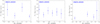 |
Fig. 3 Background-subtracted eROSITA light curves in the 0.2–2.0 keV energy band. We show the light curves for the two samples of UCDs studied in this work, the new and the literature UCDs, in Fig. A.1. |
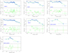 |
Fig. 4 X-ray spectra of UCDs associated with XMM-Newton (the first five panels) and eROSITA (the last two panels) sources that have more than 200 and 30 net counts, respectively. The spectra are plotted together with the best-fitting apec model and the residuals (both shown in green); see text in Sect. 3.1.3 and Table 6. |
3.1.3 X-ray spectra
We fit all EPIC/pn and eROSITA spectra with net counts >200 and net counts >30, respectively. These thresholds were set after several tests to find the best-fit parameters. They are met by 6 UCds, 5 detected with XMM-Newton and one from eRASS where it exceeds the above threshold in two out of 4 surveys.
We made use of XSPEC version 12.13 (Arnaud 1996) using a one- or two-temperature thermal APEC model. Given that nearly all observed counts are concentrated below 2.0 keV (see Sect. 3.1.1) we fit the APEC model to the spectrum in the 0.2– 2.0 keV energy band. Interstellar absorption is negligible for these nearby objects. Given the low statistics of the spectra we fixed the global abundance (Z) to 0.3 Z⊙, a typical value for stellar coronae (Maggio et al. 2007), and we adopted the solar abundance vector set from Asplund et al. (2009). The free parameters are thus, the temperatures (kT) and emission measures (EM). We calculated the 1σ uncertainties of the fit parameters using the ERROR command in XSPEC. We used the best-fit parameters to compute for each spectrum the emission measure weighted mean coronal temperature (< kTcorona >) defined as
 (1)
(1)
where kTn and EMn with n = 1,2 are the two temperatures and two emission measures of the best-fitting model.
The results of the best-fitting models are summarized for all UCDs in Table 6, where we show the values for the two kT and EM components with their 1 σ uncertainties (Cols. 2–5), the reduced χ square  and the degrees of freedom (d.o.f.) in Cols. 6 and 7 and the average coronal temperature (〈kTcorona〉) in the last column. The seven spectra, their best-fit models and the relative residuals between data and model are displayed in Fig. 4.
We use the X-ray emission properties derived from spectral fits to the five objects with more than 200 counts in the XMM-Newton data (Table 6) to construct constraints on the size scale of the thermal coronal emission. We start with the pressure equilibrium equation,
 (2)
(2)
where Beq is the equipartition magnetic field strength that balances thermal coronal pressure represented by electron density ne, and coronal temperature kBT, where kB is Boltzmann’s constant. The electron density is obtained from the volume emission measure (VEM) according to
 (3)
(3)
where V is the emitting volume. Combining Eqs. (2) and (3) and assuming that the corona is a spherical shell with height H we can derive the equipartition magnetic field strength as a function of coronal height according to
 (4)
(4)
Inspection of Table 6 shows that, while there is a significant difference between the two X-ray temperatures fitted, the volume emission measures of each component are roughly equal within the error bars. Therefore, because the hotter temperature plasma will provide a stronger constraint on the confining magnetic field, we use the temperature and emission measure values of the hotter component. The results are shown in Fig. 5 and further discussed in Sect. 5.
Best-fit X-ray spectral parameters for the five UCDs with net counts >200 detected with XMM-Newton and for the only object that shows two eROSITA detections with net counts >30.
3.1.4 X-ray luminosities
For the brightest detections for which we performed the spectral analysis, we computed the X-ray flux (ƒx) with the flux routine of XSPEC. For the fainter sources, as well as for the upper limits, we converted the count rate into flux with a conversion factor based on the results of our spectral analysis and in the 0.2– 2.0 keV energy band. Specifically, we calculated the CF of each bright target as the ratio of the XSPEC flux and the count rate from the source detection. Then we calculated the mean value.
 (5)
(5)
We adopted this approach for both instruments (EPIC/pn and eROSITA) separately, so that the instrumental properties are implicitly considered. The final CFs are CFXMM = 2.71 × 10⁻¹² ± 3.44 × 10⁻¹² erg cm−2 cts−1 and CFeR = 8.01 × 10⁻¹³ ± 7.33 × 10⁻¹⁴ erg cm−2 cts−1. We then computed X-ray luminosities (Lx) and X-ray to bolometric luminosity ratios (Lx/Lbol) for the 0.2–2.0 keV energy band using the Gaia-DR3 distances and bolometric luminosities from Table 4. The X-ray luminosity and Lx/Lbol ratios as well as their upper limits for the undetected UCDs are listed in Tables 2 and 5 for XMM-Newton and eROSITA, respectively.
To be able to compare the literature sample with that of our sample of UCDs we converted the published X-ray luminosities to the energy band chosen for this work. To this end, we calculated a CF for each energy band reported in the literature that is different from our 0.2–2.0 keV band. We used the online count rate simulator WebPIMMS5, assuming an unabsorbed 1T-apec model with temperature of 0.61 keV and coronal abundance of 0.2 Z⊙. Among the values implemented in WebPIMMS we chose 0.61 keV because it is the closest to the measured mean value, computed with the emission measure weighted temperatures of the six UCDs with spectral fits (see Sect. 3.1.3 and Table 6 for the spectral analysis). The updated X-ray literature data are shown in Table 7 with the computed CFs, the original values, and their references. In this table we report the results of observations taken while the target was in a quiescent state (upper limits are included). In Cols. 8 and 11 we indicate if a specific object has data from the literature of enhanced activity (X-ray flares and/or radio bursts). When the count rate is not provided in the literature we directly converted the literature flux from the original energy band into the 0.2–2.0 keV band, so no CF is provided in this case. Finally, we show the published quiescent and bursting radio luminosities (Lrad) and their references in the last four columns of the same table.
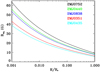 |
Fig. 5 Equipartition magnetic field strength for objects with spectral fits from XMM-Newton as a function of the assumed thickness of a spherically symmetric corona, using coronal temperatures and emission measures from Table 6 and radius measurements from Table 4. |
3.2 Radio data analysis
Observations were obtained as part of three NRAO/JVLA projects and one ATCA project; observation specifics are listed in Table 3. We note that we add in the radio flux densities for 3 of our targets which were reported previously in the literature. Table 8 lists the specific radio frequency ranges used in pre-upgrade VLA observations (pertinent to the literature references used in this paper), and the JVLA and ATCA observations presented. Our literature references are Antonova et al. (2013) for 2M0215 and Berger (2006) for 2M0440 and 2M0435. Berger (2006) does not quantify what the quoted upper limits are, and we are assuming that they are 3 sigma. We have recalculated the 3σ upper limits on the radio luminosities from the literature using Gaia-DR3 distances from Table 4. These updated values are listed in Table 9.
3.2.1 JVLA data
The flux calibrator (Col. 7 of Table 3) was used to establish both overall gain solutions as well as determine bandpass calibrations, while the phase calibrator (Col. 8 of Table 3) was used to correct for phase variations. Data editing and further calibration steps were performed using standard techniques in the Common Astronomy Software Applications (CASA) package (McMullin et al. 2007). The calibrated visibility data for each target were split off from the main dataset after successful calibration and imaged. The individual epochs of observations in January 2015 were calibrated and imaged separately, then the visibility datasets were concatenated and imaged as a whole to increase the sensitivity. A similar approach was used for the two epochs of observations in September 2020. The cell size for imaging the D configuration X-band datasets was 1.5 arc-sec, while for the CnB configuration X-band datasets the cell size was 0.34 arcsec. The cell size for the B configuration C-band datasets was 0.5 arcsec. The clean algorithm used to create images employed natural weighting with a threshold of 10 µJy to discover faint radio sources.
We derived the expected position of our targets at the time of each JVLA observation, taking into account the P.M. provided by Gaia DR3 (see Table 4). Once images had been created for each of the four fields, we searched for any radio sources in the vicinity of the expected target positions. For the six epochs of 2MJ0306 and two of 2MJ0652, we searched the image for each epoch as well as that made from combining all epochs.
The only field with a radio source near the expected target position is 2MJ0752, with a radio counterpart offset from the expected position by only 0.27″ (Fig. 6). After deconvolving from the clean beam it appears to be a point source with a peak flux density of 78.9±3.4 µJy beam–1 in total intensity. The same field imaged in Stokes V also shows a source at the same position, with a peak flux density of -59.8±2.6 µJy beam–1, or circular polarization fraction V/ƒ = –76±5%. Late-type stellar radio sources are typically the only type to experience high degrees of circular polarization. We consider the association of this highly circularly polarized radio point source with the brown dwarf robust, considering the beam size of 14.45″ × 8.2″ and the significance of the detection. For all other targets the radio sources in the images are offset by >30″ from the expected target position, that is they are undetected. The fields around the other four sources are displayed in Figs. B.1 and B.2. Table 9 lists the 3σ upper limits and the detected radio flux with rms for all of the program sources, and Table 10 describes the average, maximum and minimum values of total and circularly polarized flux.
Radio frequency coverage.
Radio flux densities (with 1σ error) or 3σ upper limit for non-detections.
3.2.2 ATCA data
Reduction and calibration of ATCA data proceeded as noted above in Sect. 3.2.1, using Miriad software (Sault et al. 1995), with amplitude and phase calibration using sources identified in Cols. 7 and 8, respectively, of Table 3. The cell size for imaging C band observations was 0.8 arcsec, while for X band observations it was 0.4 arcsec.
We performed similar calculations as described above in Sect. 3.2.1 to determine the expected position of the targets at the epoch of the observation. The only object with a confident detection was 2MJ0838, with a point source only 0.3″ away from the expected position at both X and C bands. Maps of the region around the expected position for this object in Stokes I and V are shown in Fig. 7, while those for the undetected objects are illustrated in Fig. B.3. Table 9 lists the 3σ upper limits and detected radio luminosities; the only object with a detection is 2MJ0838. Table 10 lists the average values of the flux densities for total intensity and circularly polarized emission averaged across the observation.
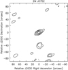 |
Fig. 6 Contour image of the JVLA field around the target 2MJ0752, which has a source only 0.27″ from the expected position. The size is 3′ × 3′ and contour levels are 3, 5, 10, 15, 20, 30, 50, and 100 times the image rms, which is listed in Table 9. |
Total and circularly polarized intensities of radio-detected objects.
3.3 TESS data
We analyzed TESS light curves with the primary aim to obtain the rotation periods of the UCDs, and secondly to identify optical flares as additional activity diagnostics. The results of the TESS analysis and TESS identification numbers (TIC) for all UCDs studied in this article, namely the 26 objects from our dedicated X-ray/radio campaigns and the literature sample, are given in Table 11.
We uploaded the target list of the UCDs to the Barbara A. Mikulski Archive for Space Telescopes (MAST) interface and found two-minute cadence light curves processed by the TESS Collaboration for 17 out of the 26 targets. Most of them were observed in multiple sectors (see Table 11), and we downloaded 69 individual light curves from MAST.
For our analysis we used the PDCSAP_FLUX, in which the pipeline processing has removed some of the instrument system-atics from the flux measurements. TESS assigns a quality flag to all measurements. In the first step, we removed all data points with a quality flag different from 0 except of ‘Impulsive outlier’ (which could be real stellar flares) and ‘Cosmic ray in collateral data’ (see more detailed information in Magaudda et al. 2022). We then normalized the individual sector light curves of each UCD by dividing all data points by the median flux. The period search was performed using the method described by Magaudda et al. (2022). In short, we used three different standard time series analysis techniques, the generalized Lomb-Scargle periodogram (GLS; Zechmeister & Kürster 2009), the autocorrelation function (ACF), and sine fitting. We then phase-folded the light curves with the best period estimate from each method. By visual inspection we selected the methods that yielded the period that best represents the light curves. As final period we adopted the mean value of these methods. If light curves from more than one sector were available for a given UCD all good period values from the different methods in the different sectors were averaged (up to three values per sector). Uncertainties on the Prot values are given as the standard deviation of those period values that were used to calculate our adopted period. The typical results of our analysis are demonstrated on an example for one sector of the UCD TIC 29890705 in Fig. C.1.
This initial period search resulted in a significant period detection for seven of 26 targets. However, by eye the ACF of 3 of the remaining UCDs without a period estimate (i.e., TIC 70555405, TIC 117733581 and TIC 401945077) appears to display a clear signal. Therefore, we decided to bin the original light curves of all 19 UCDs without a detected period with a factor of 15 and we repeated the period search. This way, we found a reliable rotation period for further 5 UCDs, including the three mentioned above.
Therefore, as a final result we were able to detect a period for 12 out of 26 UCDs. The period for one of them, TIC 308243298, is, however, only marginally detected in the binned data. The object was observed in 4 sectors but only two of them show a detection. Since this period is consistent with the period upper limit from the υ sin i measurement, we consider it when we discuss the X-ray versus radio luminosity relation for UCDs with Prot ≤ 1 day (see Sect. 5).
For the 14 UCDs without a period estimate from our method or without TESS two-minute cadence data we adopted the value listed by Crossfield (2014), who collected published measurements of photometric rotation periods for 58 UCDs. When no photometric period is available, we calculated its upper limit by using υ sin i measurements from high-resolution spectroscopic data taken from the same reference and the computed radii listed in Table 4.
For those UCDs for which we found a valid photometric rotation period we calculated the inclination of the systems by using the radii listed in Table 4 and the υ sin i measurements. These data are taken from Crossfield (2014) for all UCDs, but for one object (2MJ0752) for which no value is listed in their work thus we adopted the one from Hughes et al. (2021). For 5 UCDs υ sin i is larger than the actual rotational velocity, thus we could not retrieve a reliable inclination. We flagged these cases with “υ sin i > υrot” in Table 11 where we summarize the results of the analysis of our TESS data. In particular, Cols. 2 and 3 show the TESS ID of the UCD and the number of sectors in which it was observed, Cols. 4 and 5 list the photometric period and its reference, Col. 6 holds the literature υ sin i value, and Col. 7 the inclination.
To detect flares we applied the method that we explained in detail in Stelzer et al. (2022) and Magaudda et al. (2022). In short, we smoothed the light curves and removed all data points that deviate more than 2-σ from the smoothed light curve. The treatment was repeated three times with decreasing size of the boxcar width that was used for the smoothing. The final smoothed light curve was then subtracted from the original light curve in order to remove the rotational signal. All groups of at least three consecutive data points that deviate more than 3-σ from this ‘flat’ version of the light curve were identified as potential flares. In a 5-step validation process false positive detections were removed from this list. The validation criteria are (1) the flare event must not occur right before or after a data point gap in the light curve, (2) the flux ratio between flare maximum and last flare point must be ≥2, (3) the flare maximum cannot be the last flare point, (4) the decay time has to be longer than the rise time, and (5) a fit conducted using the flare template defined by Davenport et al. (2014) must fit the flare better than a linear fit. The UCDs with validated flares that fulfill all of the above mentioned criteria are marked in the last column of Table 11.
A detailed analysis of the TESS flares is beyond the scope of this paper. Systematic studies of large samples of flares observed with TESS on UCDs have been published (Petrucci et al. 2024). In this work we merely us the presence of optical flares as an additional activity indicator in the joint multiwavelength analysis of our sample.
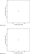 |
Fig. 7 Total intensity and Stokes V maps of the three arcminute region around the target 2MJ0838 observed with ATCA. Contours are shown at 3, 5, and 10 times the rms values listed in Table 9. |
TESS observations of all UCDs studied in this article, υ • sin i measurements retrieved from the literature and the computed inclination.
4 Objects with a particularly interesting radio behavior
4.1 2MJ0752
The source 2MJ0752 was previously reported as undetected by Berger (2006) with an upper limit of 39 µJy. Because of the high degree of circular polarization in the time- and frequency-averaged data, we explored subsets to determine whether there was any evidence of time- or frequency-dependent variability, as an indication of the bursting behavior observed in some radio-detected UCDs.
We initially explored the time domain only, creating a light curve by integrating over all spectral windows, and dividing each scan in half, to create a total of 38 time bins. The top left panel of Fig. 8 displays the time variation of total intensity and circularly polarized flux. Upper limits in total intensity are depicted as downward facing arrows. There are two local peaks in the light curve of total intensity, each having an enhancement of1.7– 1.8 times the time-integrated flux density, and separated by about 1.7 h. These however do not show up as local peaks in circularly polarized flux.
In the bottom left panel of Fig. 8, we show the percent circular polarization, computed only for time bins in which there was a detection in both total intensity and circularly polarized flux. The average value of percent circular polarization, taken from the time-averaged values of Stokes V and Stokes I flux, is shown as a black horizontal line. The high degree of circularly polarized flux obtained from the integrated maps does not reveal any significant variation over the course of the observation.
We next explored dividing the data in both time and frequency to explore spectro-temporal variations. Our initial investigation used the original 38 time bins, but subdividing the data into a few frequency bins did not reveal any significant variations. We converged on four spectral spans and six time intervals. These light curves are displayed in the right panels of Fig. 8. These again did not display evidence for significant temporal or frequency-dependent variations.
The object’s low rotational velocity of υ sin i = 9 km s–1 and rotation period of 21 .1 h measured on the TESS light curves reveal that we are seeing the UCD at the relatively high inclination angle of i ≈50◦ (see Table 11). The emission is highly circularly polarized (–76 ± 5%, see Sect. 3.2.1), which is very suggestive of bursting behavior. While the total intensity did show some variations, there was no apparent change in the amount of circular polarization. Comparison with a previous epoch of observation ~9 yr earlier, with an upper limit below the detected level of emission, suggests that the detection spanned a long-lived burst.
The light curve of 2MJ0752 across the entire band shown in Fig. 8 reveals two apparent double peaks, which at face value could be periodic bursts corresponding to a short rotation period (<2 h). However, with a known rotation period ~21 h, perhaps this observation instead reveals the leading and trailing edges of an auroral loss cone as it traverses our line of sight. The time between peaks of about 1.7 h would approximately constrain the full-width opening angle of the loss cone. And the width of each of burst, which is roughly 0.4–0.5 h, would approximately constrain the loss-cone width. Compared to previous radio detections of periodic bursting behavior that was ascribed to auroral loss cones (Hallinan et al. 2006; Yu et al. 2011), 2MJ0752 has a relatively long rotation period. Additional observations are needed to confirm that it is in fact producing periodic bursts, and to constrain the timing of the bursts at a range of frequencies. Detailed modeling of frequency- and time-dependence of the emission, along the lines of Leto et al. (2016), will likewise enable constraints on the physical properties of the emitting region.
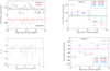 |
Fig. 8 Time series of JVLA data for 2M0752. Top left: variation of total intensity and circularly polarized flux with time integrated over all frequencies. The black and the red line denote, respectively, the time-averaged total intensity and the time-averaged amount of Stokes V flux. Bottom left: variation of the percent circular polariation integrated over all frequencies and time-average value shown as black line. Top right: time and frequency variations of the Stokes I flux density, broken up into six time bins and four frequency spans. Bottom right: variations of circularly polarized flux with the same time and frequency bins as for total flux density. |
4.2 2MJ0838
The source 2MJ0838 was detected at both C- and X-bands. In addition to a detection in total intensity (Stokes I), the source was evident in Stokes V images as well. In the C-band Stokes I image there was a strong source detected in addition to the target. We performed image fits to the sources to determine their positions and average characteristics. The average flux density values for the target, 2MJ0838, are listed in Table 10. Light curve creation proceeded in Miriad with the task UVFIT. For each invocation of the task, all source parameters for the fit to the visibility data for the specified time bin were fixed except the flux density of the target. This process was repeated individually for both Stokes I and V, and for each frequency band, to create light curves with approximately 7.5 min time bins (roughly half of each scan length). The light curves of 2MJ0838 in both radio bands as well as the time evolution of the polarization are shown in Figs. 9 and 10.
Inspection of the temporal behavior of circularly polarized and total intensity flux densities reveals interesting behavior. The C-band light curve shows evidence of total intensity variability at a factor of six at least, with additional periods where the source is undetected. The X-band light curve displays far less evidence for variability during the times when the source was detected. The average flux densities over the whole observation, derived from image fits, are overlaid as horizontal lines in Figs. 9 and 10. For both bands these averages are lower than the flux densities in time intervals when the source is detected, which reflects the significant fraction of the observing time when the source is undetected. In general, when there is a detection in the Stokes V flux density, there is little variability in these detected flux density levels. We note though that there are relatively few intervals when there is a Stokes V detection. The average values of circularly polarized flux density derived from the entire observation are smaller in an absolute value sense than the time intervals when it is detected; this mirrors the behavior noted for the average total intensity. Table 10 delineates these average, minimum, and maximum detected flux densities.
The periods of time with elevated C-band flux densities correspond in the X-band to either upper limits or to no evidence for variability. The time period 07:20:35–09:52:55 is indicative of the first type, variability at C-band with undetected flux densities at X-band, while the time period 10:59:45–12:58:25 shows no indication of variability at X-band and factors of ~three variability at C-band. We term these “C1” and “C2”, respectively.
We investigated the frequency dependence of the large and varying C-band flux during the decay phase of C2 by repeating the above calculations in each time bin but splitting the 2.048 GHz bandpass into four 512 MHz spectral intervals. We determined the flux of the bright object noted above in each spectral interval, and repeated the UVFIT calculations, allowing only the peak flux density of the target to vary. In order to investigate spectral variations, we filtered on time bins where the signal to noise ratio of the time bin across the entire C-band bandpass was larger than 8, and the signal-to-noise ratio of each of the four subbands was larger than 3. This resulted in five time bins. These times are indicated in Fig. 9 and the spectral variations, including the flux density measurement at X-band, are shown in Fig. 11.
We speculate that events C1 and C2 on 2MJ0838 are gyrosynchrotron emission from flares, since we have not detected circular polarization associated with these events as is typical for coherent bursty emission. The initial stages of the decay of C2 shown in Fig. 11 reveal a very steep frequency dependence of the flux in the first two frequency bins. We constrain the spectral index from these two bins for the first three time intervals, and overplot the fit results. This reveals that the emission from 4.5–5.5 GHz at least in these three time bins during the decay phase of C2 is consistent with a falling spectrum, possibly indicating optically thin emission. The flux densities at higher frequencies, 5.5–10 GHz, show very little variation with frequency. This constrains the peak frequency of the presumed gyrosynchrotron emission to be at a value below 4.5 GHz. We note that this value is lower than what is typically seen from solar and stellar gyrosynchrotron tlfares, which have peak frequencies 5–10 GHz or higher (Shaik & Gary 2021; Dulk 1985).
Using Eq. (39) in Dulk (1985), we explore for the C2 event of 2MJ0838 the dependence of the peak frequency on the magnetic field strength in the radio-emitting source as well as the product of the total number density of nonthermal electrons times the length scale of the radio-emitting region, denoted NL by Dulk (1985). This relationship also depends on the power-law index of the accelerated particle distribution determined from radio observations (δr) as well as an assumption about the angle of propagation with respect to the line of sight, θ (here assumed to be 45°. We use the values of spectral index α constrained from Fig. 11 to infer the index of the accelerated electron distribution δr, where α = 1.22 – 0.9δr under optically thin conditions for gyrosynchrotron emission (Eq. (35) in Dulk 1985). Time bins C2D1 and C2D2 in Fig. 11 provide bounds for the values of α and hence δr. For these time bins we find δr = 8.8 ± 2.6 and δr = 5.2 ± 2.4, respectively. Figure 12 shows the relationships among these parameters for a wide range of B and NL; we have assumed that the angle of propagation θ is 45° for these parameter space calculations. Based on recent studies of solar flares the nonthermal electron density appears to range between 105 and 1011 cm–3 (Fleishman et al. 2022), and loop sizes from solar to stellar flares can range from ≤108 cm (Cargill & Klimchuk 2006) to the size of the stellar diameter (Stelzer et al. 2006). We use a wide range of parameter space for N and L to investigate trends. Inspection of Fig. 12 shows that in combination with the peak frequency constraints, the lower value of δr is more constraining on allowed regions of magnetic field strength. In particular, magnetic field strengths of only a few tens of Gauss are compatible with a nonthermal electron density near the maximum found in Fleishman et al. (2022) (1011 cm–3) and a length scale of order the radius of 2MJ0838 (1010 cm). This is similar to the equiparti-tion field strength derived from X-ray observations in Sect. 3.1.3, but whereas the X-ray constraints are determined from the average coronal properties, the current constraints derive from a specific event corresponding to elevated flux levels and are not necessarily characteristic. Additional modeling will be needed to constrain these parameters further.
The circular polarization properties of 2MJ0838 are intriguing. They do not appear to be periodic; the detections at both X and C bands are just slightly above 3σ. Additionally, they indicate moderate degrees of circular polarization (40–50%) when there is a detection, which is different from the highly circularly polarized bursts seen in 2MJ0752 and other UCDs which approach 100% circular polarization. This is also a much larger value of circular polarization fraction than is typically seen from quiescent gyrosynchrotron emission, generally ~20% or less (White et al. 1989). If we identify the frequencies at which the circular polarization is detected with the electron gyro-frequency, then we can place a constraint on the magnetic field strength in the steady radio-emitting region, with νobs = s • νB, where s is the harmonic number of the emission being observed, and νB is the gyrofrequency, νB ≈ 2.8 × 10⁶B[G] Hz. The large frequencies at which we detected the circular polarization, namely 9000 MHz, imply field strengths of one to several kilogauss.
We use the method described by Osten et al. (2016); Smith et al. (2005) to convert the radio light curve into a constraint on the nonthermal energy as a function of magnetic field strength in the radio-emitting source and the distribution of accelerated particles δr as derived above. This contour plot is displayed in Fig. 13. While we do not have simultaneous measures of radiated flare energy, we note that this range spans 1030–1034 erg for values of δr consistent with the observational constraints; these are flare energy ranges noted from a recent analysis of TESS white light flares on ultracool dwarfs (Petrucci et al. 2024). For realistic flare energies (Fig. 13) the magnetic field in the flaring source is on the order of a few 100 G, or less.
The equipartition field, derived from average X-ry measurements of this object in Sect. 3.1.3, is considerably smaller than what is derived from the flare analysis. On its face, this implies that these coronae could be extremely compact. An apt comparison is that of Ness et al. (2004), whose analysis of X-ray grating data of late-type stars combined measurements of electron density and volume emission measures, to suggest “pathologically small” coronal scale heights of 107 cm or less (H/R★ < 0.001 for the M dwarfs considered in their sample). They invoke a filling factor less than unity to overcome this situation. Constraints on the sizes of coronae of other late-type stars indicate larger extents: X-ray eclipses of the G dwarf component in the α CrB system by its X-ray dark A star companion reveal a coronal height above the limb less than a solar radius (Schmitt & Kurster 1994). Similarly, imaging observations of the Sun reveal a uniform typical height of the bright portion of the solar corona to ~0.3 R⊙ (DeForest 2007).
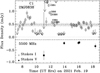 |
Fig. 9 Total intensity and circular polarization behavior of 2MJ0838 with ATCA at C band. Light curve bin size is 7.5 min. Open squares indicate detections of total intensity, and filled symbols indicate detections of circularly polarized flux density. For upper limits in total intensity, an arrow from 1σ to 3σ is shown. The dashed lines and forward (backward) hatched regions indicate the average flux density and standard deviation for total intensity (circularly polarized flux) determined from image analysis spanning the entire time. Approximate extent of events “C1” and “C2” are indicated. Specific time bins in the decay phase of event C2 are denoted, and their spectral energy distributions are plotted in Fig. 11. |
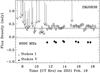 |
Fig. 10 Total intensity and circular polarization behavior for 2MJ0838 at X band. Figure labels are the same as for Fig. 9. |
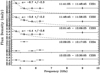 |
Fig. 11 Spectra of individual time bins during the decay phase of event C2 on SCR 0838 noted in Fig. 9. The C-band was divided into four spectral bins for which the flux was computed, while the X-band is represented by a single flux measurement. The spectral index calculated from the two lowest frequency bins is shown for the first three time bins in the decay of C2. |
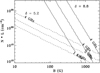 |
Fig. 12 Contour plot of dependence of the peak frequency of gyrosyn-chrotron emission as a function of magnetic field strength in the radio-emitting source and the product of total number density of accelerated electrons and size scale of the emission NL. Two different sets of contours are shown, which bracket the inferred values of δr seen in the frequency-dependent decay of event C2 in SCR0838 shown in Fig. 11. The larger values of NL provide more constraints on the field strength in the radio-emitting region, in order to be consistent with the low peak frequency and the smaller value of δr. |
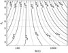 |
Fig. 13 Contour plot of estimated nonthermal energy in radio flare C2 seen on SCR0838, as a function of the magnetic field strength (B) in the radio emitting region and the power-law index of the distribution of accelerated particles, δr. Horizontal lines indicate the range of δr from the frequency dependence in Fig. 11. |
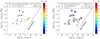 |
Fig. 14 Radio vs. X-ray luminosity. Left panel: the lowest measured X-ray luminosity in the 0.2–2.0 keV energy band, including upper limits. The black line represents the relation from Güdel & Benz (1993). Right panel: same as left panel with the radio bursts and X-ray flares presented as open squares and stars, respectively. See Sect. 5 for more details. |
5 Discussion
With our increased database of UCDs with sensitive X-ray and radio data we present an updated view of the LR,ν–Lx relation (Fig. 14). If multiple observations were obtained in either waveband we show the most sensitive one (left panel), including upper limits in case of non-detections. Radio and X-ray upper limits are displayed with filled upside-down and left-oriented triangles, respectively, while upper limits in both bands are presented with smaller filled diamonds and full detections with filled circles. In the right panel of Fig. 14, we highlight objects for which X-ray flares and radio bursts have been observed in at least one instance. Among all objects of this work, 26 UCDs including the literature sample, we detected optical flares for 9 objects, among which 4 show X-ray flaring activity, 3 emitted radio bursts, and only 2 present activity along all three wavelength bands. For the UCDs from our dedicated campaigns whether there is X-ray flaring activity or not is inferred from the variability in the XMM-Newton light curves (Fig. 2). This choice is justified by the fact that the time resolution of XMM-Newton is higher than the one of eROSITA, that we recall being only 4 h and, thus, longer than typical X-ray flares on UCDs (see e.g. Stelzer et al. 2006). Since we have one radio observation for each target, we account for variability simply if there is a burst in their emission. For the literature sample, instead, we adopted the notion of flaring or bursting versus quiescent X-ray and radio activity as presented in the references. In both panels of Fig. 14 we also show the GB relation (see Sect. 1 for more details).
We confirm previous findings that UCDs are drastically offset from the GB relation. With our enhanced sample statistics we overall confirm the picture of two groups of UCDs with different activity characteristics outlaid by Stelzer et al. (2012), with X-ray flaring objects being closer to the GB relation and radio bursting ones often associated with faint or no measurable X-ray emission. The majority of the joint X-ray/radio sample is detected in X-rays and at levels of Lx fainter than the stars on which the GB relation was defined (the dashed part of the line in Fig. 15). This (apparently) leftwards displacement with respect to the GB relation could be explained by the lack of sensitivity at radio wavelengths. The color code of this figure shows that radio bursts are mostly detected from fast-rotating UCDs in agreement with the results of Pineda et al. (2017). Their two regimes of fast-rotating “radio-loud” and slow-rotating “radio-quiet” UCDs were the basis of our target selection (see Sect. 1). Since we work with photometric period while Pineda et al. (2017) used v sin i measurements, we had translated their boundary between the two regimes (υ sin i ≈ 38 km s–1) to a value of Prot ≈ 0.2 day (assuming a typical late-M dwarf radius of R★ ~ 0.15 R⊙ and i ≈ 90º). In contrast, X-ray flares are found on UCDs that are distributed throughout the range of rotation periods considered in Fig. 14, implying no evident relation for UCDs between their X-ray activity and rotation.
The X-ray scale height and equipartition magnetic field analysis in Sect. 3.1.3 reveals either a very compact corona for values of magnetic field strength of a few tens of Gauss, or extremely low confining magnetic field strength for a more extended corona. This could originate from the assumptions of homogeneity and spherical symmetry.
One UCD of our sample (2MJ0752) is simultaneously detected along the two wavebands adopted for this work and its X-ray emission is one of the brightest. We do not infer X-ray variability from the XMM-Newton light curve (see Fig. 2), although we clearly see variable X-ray emission from eROSITA detections (see Fig. 3). In Sect. 4.1 and Fig. 8, we presented the radio light curve of this UCD that shows two apparent double peaks. This brightness modulation suggests the presence of a periodic burst corresponding to a shorter rotation period (<2 h) than the one of 2MJ0752 (listed in Table 11). We linked this radio emission to a possible auroral electron precipitation, as the one typical of giant planets of the solar system. The X-ray brightest and radio simultaneous detections of this UCD are showing signatures expected from higher-mass M dwarfs along with emerging evidence of radio auroral emission, reinforcing the hypothesis of a bimodal dynamo mechanism ruling the X-ray/radio activity along the ultracool dwarf regime.
For a direct investigation of the dependence of radio and X-ray activity on rotation we show in Fig. 15 the relation between LR,v/LX and Prot, emphasizing objects for which an X-ray flare (open star), optical flare (open circle) or a radio burst (open square) is present in our dataset. UCDs that are upper limits in both X-ray and radio bands are placed on the bottom of the plotting window, and we indicate with left-oriented arrows the rotation periods that are upper limits, calculated from v sin i measurements. In this LR,ν/Lx–Prot space the GB relation is a horizontal line, and we placed a vertical solid line at Prot = 0.2 day to separate the radio-loud and radio-quiet regimes from Pineda et al. (2017).
Since only 2 of the 26 UCDs experienced activity along all three wavelengths, searching for a relation between the mechanism that generates a radio bursts rather than an optical or X-ray flare remains a difficult task. Thus, a larger sample and B measurements are required and in order to investigate such dichotomy that might be caused by the structure of the magnetic field.
Given the fast rotation of UCDs and their peculiar X-ray/radio behavior it is interesting to study their position in the rotation-activity relation compared to earlier M dwarfs. We use the representation in terms of fractional luminosity, Lx/Lbol versus Prot (see Fig. 16). The Lx/Lbol ratio has the advantage of removing most of the mass dependence of X-ray brightness in the saturated regime. In most studies of the activity-rotation relation this parameter is combined with the Rossby number (R0 = τconv/Prot, where τconv is the convective timescale). For late-type stars activity-rotation relations that make use of the Rossby number display a smaller horizontal spread than those involving only Prot (Wright et al. 2011; Magaudda et al. 2020). However, since the convective timescale is notoriously difficult to constrain and no parametrizations exist for UCDs later than SpT = M9 we work with the rotation period. In Fig. 16, the SpT-color code applies to both the UCDs from this article and the comparison sample of early to mid-M dwarfs from Magaudda et al. (2020, 2022), but for clarity we additionally highlight the UCDs with open black circles. As in the other figures, we display for the UCDs the most sensitive X-ray measurement, including the upper limits that are plotted as upside-down open triangles. The left-oriented arrows indicate for which object we calculated the rotation period from v sin i measurements. As stated in many previous works (Wright et al. 2011, 2018; Wright & Drake 2016; Stelzer et al. 2016; González-Álvarez et al. 2019; Magaudda et al. 2020, 2022), the activity rotation relation of early to mid-M dwarfs splits into two regimes: for Prot ⪅ 10 days the X-ray activity does not depend on the rotation (saturated regime) and at longer periods the X-ray activity declines with increasing rotational period (unsaturated or 'correlated' regime).
For our analysis of the Lx/Lbol–Prot relation we only consider the quiescent state of our sample. Our sample of late-M dwarfs spans the entire range of Lx/Lbol that covers the typical activity level of both the saturated and unsaturated regime of the earlier SpTs from Magaudda et al. (2022). This spread and consequent low activity of UCDs evidently show a lack of correlation between Lx and Prot, and it is usually ascribed to their mostly neutral atmospheres, that – even if the magnetic field is present – do not allow coupling with matter and thus outer magnetic heated atmospheres are not prominent (Mohanty et al. 2002). Previous works already found a significant drop in X-ray activity beyond spectral type ~M7 (Cook et al. 2014; Berger et al. 2010). Specifically, Berger et al. (2010) showed Lx/Lbol ≈ 10–4 for M7-M9 and Lx/Lbol ≈ 10–5 as deepest limits for L dwarfs, while Cook et al. (2014) found a Lx/Lbol-spread of 2 dex for UCDs located in the saturated regime, that is Prot ≤ 10 days. We found a Lx/Lbol-spread for UCDs with Prot ≤ 1 day larger than the one presented in Cook et al. (2014) only for quiescent X-ray emissions (see Fig. 16). In fact, we observe a declining Lx/Lbol for later SpT than M7 down to Lx/Lbol ≈ 3 × 10⁻⁶. This detection refers to a M9 dwarf from the literature, DENIS J1048, for which the deepest Lx is from XMM-Newton observation (see Tables 7 and 5). Furthermore, with our larger and updated sample of UCDs we confirm the results of Cook et al. (2014), whereby the authors coupled the decrease in X-ray activity of rapidly rotating UCDs with a decrease in the effectiveness of the magnetic dynamo. Cook et al. (2014) suggested that the X-ray activity decrease for UCDs is due to the presence of a bimodal dynamo across late-type dwarfs that produces distinct magnetic field topologies. In other words, UCDs with large-scale fields may spin down more efficiently than those with weaker and tangled fields.
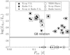 |
Fig. 15 Radio to X-ray luminosity ratio vs. the rotation period. TESS and X-ray flares are shown with open filled circles and stars, respectively, while radio bursts with open filled squares. UCDs that are placed on the x-axis are undetected with both X-ray and radio instruments. The solid horizontal line at log(LR,v/Lx) 15.5 represents the relation of Güdel & Benz (1993) as a function of Prot, while the vertical line at Prot = 0.2 day is from Pineda et al. (2017) to separate the radio-loud from the radio-quiet regime. |
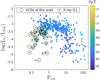 |
Fig. 16 Activity-rotation relation in terms of Lx/Lbol vs. Prot and based on the SpT-color code. As in Figs. 14 and 15, we present the deepest X-ray luminosity, including the upper limits (upside-down open tria-gles) as a function of rotation periods extracted from TESS light curves or calculated from υ • sin i measurements when the rotational modulation do not provide a clear value (left-oriented arrows). The UCD sample of this work (open circles) is compared with the M dwarfs studied in Magaudda et al. (2020, 2022), see Sect. 5. |
6 Conclusions
We present a collection of simultaneous X-ray/radio observations of a sample of ten UCDs that we enlarge with archival X-ray and radio data from the literature. The final sample counts 26 late-M dwarfs. We added two more radio-detected dwarfs to the list of known emitters: 2MJ0752 and 2MJ0838. The first object is a slow rotating (υ sin i = 9 km s–1) and one of the X-ray brightest radio-detected UCDs. It exhibits a possible loss cone along the line of sight, suggested by the presence of two double peaks in its radio light curve that correspond to a rotation period shorter than the one extracted from TESS data (Prot = 0.88 day). Given that there is a bias in radio detection fraction against the slowest rotating UCDs (McLean et al. 2012; Stelzer et al. 2012), it becomes an even more intriguing object to follow up. The detection of this target during what looks like a long-lasting radio burst, after a previous epoch in which a lower upper limit was obtained, suggests that the actual fraction of radio-emitting objects amongst UCDs is much higher than one would estimate based on single epochs alone. The other radio-detected object (2MJ0838) displays evidence for X-ray emission and incoherent radio flares, along with a moderate circularly polarized flux which does not vary appreciably. We speculate that this object is experiencing a transition in its magnetic behavior, producing signatures typical of higher-mass M dwarfs along with emerging evidence of auroral emission.
We updated the LR,ν –Lx relation for UCDs with rotation periods lower than 1 day. While comparing our results with those from Güdel & Benz (1993) for earlier-type stars we confirmed that rapid rotators lie the furthest away from the GB relation, and are more likely to exhibit radio bursts indicative of loss cone-auroral emission. Paudel et al. (2018) noted the ubiquity of white-light flaring in UCDs. Our results support and extend this conclusion to shorter wavebands by noting that X-ray flaring occurs throughout the region of radio and X-ray luminosities in Fig. 14, while objects with radio bursts tend to be experienced more by fast rotating UCDs. Based on our examination of radio, X-ray and rotation period results we observed and confirmed the presence of a radio-loud regime for UCDs with Prot ≤ 0.2 day, already proposed by Pineda et al. (2017), and a radio-quiet regime where most of the X-ray flares take place for larger Prot.
Finally, we examined Lx/Lbol as a function of Prot for our sample of UCDs in comparison with the results of Magaudda et al. (2022) for earlier-type M dwarfs. We observed that despite their fast rotation the X-ray emission of UCDs covers the whole Lx/Lbol range (≈ –3.0… – 5.5) that comprises the saturated and the unsaturated regimes of earlier M dwarfs. This shows that no evident relation seems to emerge between the X-ray emission of UCDs with respect to their rotation. The low activity detected for our sample of UCDs can be ascribed to their mostly neutral atmospheres, that do not allow coupling with matter (Mohanty et al. 2002) and to a decrease of dynamo efficiency that suggests the presence of a bimodal dynamo across late-type dwarfs that changes the magnetic field topology (Cook et al. 2014).
Acknowledgements
E.M. is supported by Deutsche Forschungsgemeinschaft under grant STE 1068/8-1. This work is based on data from eROSITA, the soft X-ray instrument aboard SRG, a joint Russian-German science mission supported by the Russian Space Agency (Roskosmos), in the interests of the Russian Academy of Sciences represented by its Space Research Institute (IKI), and the Deutsches Zentrum für Luft- und Raumfahrt (DLR). The SRG spacecraft was built by Lavochkin Association (NPOL) and its subcontractors, and is operated by NPOL with support from the Max Planck Institute for Extraterrestrial Physics (MPE). The development and construction of the eROSITA X-ray instrument was led by MPE, with contributions from the Dr. Karl Remeis Observatory Bamberg and ECAP (FAU Erlangen-Nuernberg), the University of Hamburg Observatory, the Leibniz Institute for Astrophysics Potsdam (AIP), and the Institute for Astronomy and Astrophysics of the University of Tübingen, with the support of DLR and the Max Planck Society. The Argelander Institute for Astronomy of the University of Bonn and the Ludwig Maximilians Universität Munich also participated in the science preparation for eROSITA. The eROSITA data shown here were processed using the eSASS/NRTA software system developed by the German eROSITA consortium. This paper includes data collected with the TESS mission, obtained from the MAST data archive at the Space Telescope Science Institute (STScI). Funding for the TESS mission is provided by the NASA Explorer Program. STScI is operated by the Association of Universities for Research in Astronomy, Inc., under NASA contract NAS 5–26555.
Appendix A eROSITA light curves
We show the continuation of Fig. 3 in Sect. 3.1.2 for the remaining UCDs studied in this work.
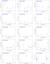 |
Fig. A.1 Background-subtracted eROSITA light curves of the two samples presented in this work, the new and the literature UCDs in the 0.2– 2.0 keV energy band. Continued from Fig. 3 in Sect. 3.1.2. |
Appendix B Radio maps
The Appendix displays radio maps of the field around objects which did not produce a detection at radio wavelengths.
 |
Fig. B.1 Contour images of the JVLA field around the three JVLA targets in the D and CnB configuration as observed at the X band that were not detected. The size is 3′ × 3′ for the two first images taken in D configuration and 2.6′ × 2.6′ for the last one observed in CnB configuration. Contour levels are 3, 5, 10, 15, 20, 30, 50, and 100 times the image rms, which is listed in Table 9. The right ascension and declination of the phase center for the observation for each target is listed in Table 3. |
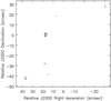 |
Fig. B.2 Zoom-in of the region around 2MJ0652 with JVLA as observed at the C band. Contours are 5, 8, and 10 times the rms of 1.8µJy determined from a blank region of the field. |
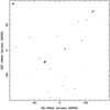 |
Fig. B.3 Maps of the three-arcminute region around the lower frequency of the targets 2MJ1055 observed with ATCA, which was not detected at either frequency. Contours are shown at 3, 5, and 10 times the rms values listed in Table 9. |
Appendix C Rotation analysis
We present an example of our TESS rotation analysis showing the results we obtained for the UCD TIC 29890705.
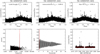 |
Fig. C.1 Result of the period search for TIC 298907057 observed with TESS in sector 32: from left to right, the results refer to the Lomb-Scargle periodogram, auto-correlation, and sine-fitting. top panels - light curves phase-folded with the periods obtained with each of the different methods; bottom - periodogram, autocorrelation function and the original light curve with the sine fit. |
References
- Antonova, A., Doyle, J. G., Hallinan, G., Golden, A., & Koen, C. 2007, A&A, 472, 257 [NASA ADS] [CrossRef] [EDP Sciences] [Google Scholar]
- Antonova, A., Hallinan, G., Doyle, J. G., et al. 2013, A&A, 549, A131 [NASA ADS] [CrossRef] [EDP Sciences] [Google Scholar]
- Arnaud, K. A. 1996, in ASP Conf. Ser., 101, Astronomical Data Analysis Software and Systems V, eds. G. H. Jacoby, & J. Barnes, 17 [NASA ADS] [Google Scholar]
- Asplund, M., Grevesse, N., Sauval, A. J., & Scott, P. 2009, ARA&A, 47, 481 [NASA ADS] [CrossRef] [Google Scholar]
- Audard, M., Osten, R. A., Brown, A., et al. 2007, A&A, 471, L63 [NASA ADS] [CrossRef] [EDP Sciences] [Google Scholar]
- Berger, E. 2002, ApJ, 572, 503 [NASA ADS] [CrossRef] [Google Scholar]
- Berger, E. 2006, ApJ, 648, 629 [NASA ADS] [CrossRef] [Google Scholar]
- Berger, E., Rutledge, R. E., Reid, I. N., et al. 2005, ApJ, 627, 960 [NASA ADS] [CrossRef] [Google Scholar]
- Berger, E., Basri, G., Gizis, J. E., et al. 2008, ApJ, 676, 1307 [NASA ADS] [CrossRef] [Google Scholar]
- Berger, E., Basri, G., Fleming, T. A., et al. 2010, ApJ, 709, 332 [Google Scholar]
- Browning, M. K. 2008, ApJ, 676, 1262 [Google Scholar]
- Brunner, H., Liu, T., Lamer, G., et al. 2022, A&A, 661, A1 [NASA ADS] [CrossRef] [EDP Sciences] [Google Scholar]
- Burgasser, A. J., & Putman, M. E. 2005, ApJ, 626, 486 [NASA ADS] [CrossRef] [Google Scholar]
- Cargill, P. J., & Klimchuk, J. A. 2006, ApJ, 643, 438 [NASA ADS] [CrossRef] [Google Scholar]
- Climent, J. B., Guirado, J. C., Pérez-Torres, M., Marcaide, J. M., & Peña-Moñino, L. 2023, Science, 381, 1120 [NASA ADS] [CrossRef] [Google Scholar]
- Cook, B. A., Williams, P. K. G., & Berger, E. 2014, ApJ, 785, 10 [NASA ADS] [CrossRef] [Google Scholar]
- Crossfield, I. J. M. 2014, A&A, 566, A130 [NASA ADS] [CrossRef] [EDP Sciences] [Google Scholar]
- Cutri, R. M., Skrutskie, M. F., van Dyk, S., et al. 2003, VizieR Online Data Catalog: II/246 [Google Scholar]
- Davenport, J. R. A., Hawley, S. L., Hebb, L., et al. 2014, ApJ, 797, 122 [Google Scholar]
- DeForest, C. E. 2007, ApJ, 661, 532 [NASA ADS] [CrossRef] [Google Scholar]
- Dulk, G. A. 1985, ARA&A, 23, 169 [Google Scholar]
- Filippazzo, J. C., Rice, E. L., Faherty, J., et al. 2015, ApJ, 810, 158 [Google Scholar]
- Fleishman, G. D., Nita, G. M., Chen, B., Yu, S., & Gary, D. E. 2022, Nature, 606, 674 [NASA ADS] [CrossRef] [Google Scholar]
- Fleming, T. A., Giampapa, M. S., Schmitt, J. H. M. M., & Bookbinder, J. A. 1993, ApJ, 410, 387 [NASA ADS] [CrossRef] [Google Scholar]
- Fleming, T. A., Schmitt, J. H. M. M., & Giampapa, M. S. 1995, ApJ, 450, 401 [NASA ADS] [CrossRef] [Google Scholar]
- Fleming, T. A., Giampapa, M. S., & Schmitt, J. H. M. M. 2000, ApJ, 533, 372 [NASA ADS] [CrossRef] [Google Scholar]
- Fleming, T. A., Giampapa, M. S., & Garza, D. 2003, ApJ, 594, 982 [NASA ADS] [CrossRef] [Google Scholar]
- Gaia Collaboration (Vallenari, A., et al.) 2023, A&A, 674, A1 [NASA ADS] [CrossRef] [EDP Sciences] [Google Scholar]
- Gillon, M., Triaud, A. H. M. J., Demory, B.-O., et al. 2017, Nature, 542, 456 [NASA ADS] [CrossRef] [Google Scholar]
- González-Álvarez, E., Micela, G., Maldonado, J., et al. 2019, A&A, 624, A27 [NASA ADS] [CrossRef] [EDP Sciences] [Google Scholar]
- Güdel, M., & Benz, A. O. 1993, ApJ, 405, L63 [NASA ADS] [CrossRef] [Google Scholar]
- Gudel, M., Schmitt, J. H. M. M., Bookbinder, J. A., & Fleming, T. A. 1993, ApJ, 415, 236 [CrossRef] [Google Scholar]
- Günther, M. N., Zhan, Z., Seager, S., et al. 2020, AJ, 159, 60 [Google Scholar]
- Hallinan, G., Antonova, A., Doyle, J. G., et al. 2006, ApJ, 653, 690 [NASA ADS] [CrossRef] [Google Scholar]
- Hallinan, G., Antonova, A., Doyle, J. G., et al. 2008, ApJ, 684, 644 [Google Scholar]
- Hughes, A. G., Boley, A. C., Osten, R. A., White, J. A., & Leacock, M. 2021, AJ, 162, 43 [NASA ADS] [CrossRef] [Google Scholar]
- Johnstone, C. P., Bartel, M., & Güdel, M. 2021, A&A, 649, A96 [EDP Sciences] [Google Scholar]
- Kao, M. M., Hallinan, G., Pineda, J. S., et al. 2016, ApJ, 818, 24 [NASA ADS] [CrossRef] [Google Scholar]
- Kao, M. M., Mioduszewski, A. J., Villadsen, J., & Shkolnik, E. L. 2023, Nature, 619, 272 [NASA ADS] [CrossRef] [Google Scholar]
- Krishnamurthi, A., Leto, G., & Linsky, J. L. 1999, AJ, 118, 1369 [NASA ADS] [CrossRef] [Google Scholar]
- Leto, P., Trigilio, C., Buemi, C. S., et al. 2016, MNRAS, 459, 1159 [NASA ADS] [CrossRef] [Google Scholar]
- Linsky, J. L. 2017, ARA&A, 55, 159 [Google Scholar]
- Lynch, C., Murphy, T., Ravi, V., et al. 2016, MNRAS, 457, 1224 [NASA ADS] [CrossRef] [Google Scholar]
- Magaudda, E., Stelzer, B., Covey, K. R., et al. 2020, A&A, 638, A20 [NASA ADS] [CrossRef] [EDP Sciences] [Google Scholar]
- Magaudda, E., Stelzer, B., Raetz, S., et al. 2022, A&A, 661, A29 [NASA ADS] [CrossRef] [EDP Sciences] [Google Scholar]
- Maggio, A., Flaccomio, E., Favata, F., et al. 2007, ApJ, 660, 1462 [NASA ADS] [CrossRef] [Google Scholar]
- McLean, M., Berger, E., & Reiners, A. 2012, ApJ, 746, 23 [Google Scholar]
- McMullin, J. P., Waters, B., Schiebel, D., Young, W., & Golap, K. 2007, in ASP Conf. Ser., 376, Astronomical Data Analysis Software and Systems XVI, eds. R. A. Shaw, F. Hill, & D. J. Bell, 127 [NASA ADS] [Google Scholar]
- Merloni, A., Larmer, G., Liu, T., et al. 2024, A&A, 682, A34 [NASA ADS] [CrossRef] [EDP Sciences] [Google Scholar]
- Mohanty, S., & Basri, G. 2003, ApJ, 583, 451 [NASA ADS] [CrossRef] [Google Scholar]
- Mohanty, S., Basri, G., Shu, F., Allard, F., & Chabrier, G. 2002, ApJ, 571, 469 [NASA ADS] [CrossRef] [Google Scholar]
- Morley, C. V., Kreidberg, L., Rustamkulov, Z., Robinson, T., & Fortney, J. J. 2017, ApJ, 850, 121 [Google Scholar]
- Murray, C. A., Queloz, D., Gillon, M., et al. 2022, MNRAS, 513, 2615 [NASA ADS] [CrossRef] [Google Scholar]
- Ness, J. U., Güdel, M., Schmitt, J. H. M. M., Audard, M., & Telleschi, A. 2004, A&A, 427, 667 [NASA ADS] [CrossRef] [EDP Sciences] [Google Scholar]
- Newton, E. R., Irwin, J., Charbonneau, D., et al. 2017, ApJ, 834, 85 [Google Scholar]
- Nichols, J. D., Burleigh, M. R., Casewell, S. L., et al. 2012, ApJ, 760, 59 [Google Scholar]
- Osten, R. A., Kowalski, A., Drake, S. A., et al. 2016, ApJ, 832, 174 [Google Scholar]
- Paudel, R. R., Gizis, J. E., Mullan, D. J., et al. 2018, ApJ, 858, 55 [Google Scholar]
- Petrucci, R. P., Gómez Maqueo Chew, Y., Jofré, E., Segura, A., & Ferrero, L. V. 2024, MNRAS, 527, 8290 [Google Scholar]
- Phan-Bao, N., Osten, R. A., Lim, J., Martín, E. L., & Ho, P. T. P. 2007, ApJ, 658, 553 [NASA ADS] [CrossRef] [Google Scholar]
- Pineda, J. S., & Hallinan, G. 2018, ApJ, 866, 155 [NASA ADS] [CrossRef] [Google Scholar]
- Pineda, J. S., Hallinan, G., & Kao, M. M. 2017, ApJ, 846, 75 [Google Scholar]
- Pineda, J. S., Youngblood, A., & France, K. 2021, ApJ, 911, 111 [NASA ADS] [CrossRef] [Google Scholar]
- Predehl, P., Andritschke, R., Arefiev, V., et al. 2021, A&A, 647, A1 [EDP Sciences] [Google Scholar]
- Ravi, V., Hallinan, G., Hobbs, G., & Champion, D. J. 2011, ApJ, 735, L2 [NASA ADS] [CrossRef] [Google Scholar]
- Ricker, G. R., Winn, J. N., Vanderspek, R., et al. 2015, J. Astron. Telescopes Instrum. Syst., 1, 014003 [Google Scholar]
- Robrade, J., & Schmitt, J. H. M. M. 2008, A&A, 487, 1139 [NASA ADS] [CrossRef] [EDP Sciences] [Google Scholar]
- Rodríguez-Barrera, M. I., Helling, C., Stark, C. R., & Rice, A. M. 2015, MNRAS, 454, 3977 [Google Scholar]
- Rose, K., Pritchard, J., Murphy, T., et al. 2023, ApJ, 951, L43 [NASA ADS] [CrossRef] [Google Scholar]
- Route, M., & Wolszczan, A. 2012, ApJ, 747, L22 [NASA ADS] [CrossRef] [Google Scholar]
- Rutledge, R. E., Basri, G., Martín, E. L., & Bildsten, L. 2000, ApJ, 538, L141 [NASA ADS] [CrossRef] [Google Scholar]
- Sault, R. J., Teuben, P. J., & Wright, M. C. H. 1995, in ASP Conf. Ser., 77, Astronomical Data Analysis Software and Systems IV, eds. R. A. Shaw, H. E. Payne, & J. J. E. Hayes, 433 [NASA ADS] [Google Scholar]
- Saur, J., Willmes, C., Fischer, C., et al. 2021, A&A, 655, A75 [NASA ADS] [CrossRef] [EDP Sciences] [Google Scholar]
- Schmitt, J. H. M. M., & Kurster, M. 1994, in ASP Conf. Ser., 64, Cool Stars, Stellar Systems, and the Sun, ed. J.-P. Caillault, 137 [NASA ADS] [Google Scholar]
- Schmitt, J. H. M. M., & Liefke, C. 2002, A&A, 382, L9 [NASA ADS] [CrossRef] [EDP Sciences] [Google Scholar]
- Shaik, S. B., & Gary, D. E. 2021, ApJ, 919, 44 [NASA ADS] [CrossRef] [Google Scholar]
- Shulyak, D., Reiners, A., Engeln, A., et al. 2017, Nat. Astron., 1, 0184 [NASA ADS] [CrossRef] [Google Scholar]
- Smith, K., Güdel, M., & Audard, M. 2005, A&A, 436, 241 [NASA ADS] [CrossRef] [EDP Sciences] [Google Scholar]
- Solanki, S. K., Inhester, B., & Schüssler, M. 2006, Rep. Progr. Phys., 69, 563 [CrossRef] [Google Scholar]
- Stelzer, B. 2004, ApJ, 615, L153 [NASA ADS] [CrossRef] [Google Scholar]
- Stelzer, B., Schmitt, J. H. M. M., Micela, G., & Liefke, C. 2006, A&A, 460, L35 [NASA ADS] [CrossRef] [EDP Sciences] [Google Scholar]
- Stelzer, B., Alcalá, J., Biazzo, K., et al. 2012, A&A, 537, A94 [NASA ADS] [CrossRef] [EDP Sciences] [Google Scholar]
- Stelzer, B., Damasso, M., Scholz, A., & Matt, S. P. 2016, MNRAS, 463, 1844 [NASA ADS] [CrossRef] [Google Scholar]
- Stelzer, B., Bogner, M., Magaudda, E., & Raetz, S. 2022, A&A, 665, A30 [NASA ADS] [CrossRef] [EDP Sciences] [Google Scholar]
- Sunyaev, R., Arefiev, V., Babyshkin, V., et al. 2021, A&A, 656, A132 [NASA ADS] [CrossRef] [EDP Sciences] [Google Scholar]
- Tagliaferri, G., Doyle, J. G., & Giommi, P. 1990, A&A, 231, 131 [NASA ADS] [Google Scholar]
- Turnpenney, S., Nichols, J. D., Wynn, G. A., & Casewell, S. L. 2017, MNRAS, 470, 4274 [Google Scholar]
- Vedantham, H. K., Callingham, J. R., Shimwell, T. W., et al. 2020, ApJ, 903, L33 [Google Scholar]
- West, A. A., Hawley, S. L., Bochanski, J. J., et al. 2008, AJ, 135, 785 [Google Scholar]
- White, S. M., Jackson, P. D., & Kundu, M. R. 1989, ApJS, 71, 895 [Google Scholar]
- Williams, P. K. G., Cook, B. A., & Berger, E. 2014, ApJ, 785, 9 [Google Scholar]
- Williams, P. K. G., Berger, E., Irwin, J., Berta-Thompson, Z. K., & Charbonneau, D. 2015, ApJ, 799, 192 [NASA ADS] [CrossRef] [Google Scholar]
- Wright, N. J., & Drake, J. J. 2016, Nature, 535, 526 [Google Scholar]
- Wright, N. J., Drake, J. J., Mamajek, E. E., & Henry, G. W. 2011, ApJ, 743, 48 [Google Scholar]
- Wright, N. J., Newton, E. R., Williams, P. K. G., Drake, J. J., & Yadav, R. K. 2018, MNRAS, 479, 2351 [Google Scholar]
- Yu, S., Hallinan, G., Doyle, J. G., et al. 2011, A&A, 525, A39 [NASA ADS] [CrossRef] [EDP Sciences] [Google Scholar]
- Zarka, P. 2007, Planet. Space Sci., 55, 598 [Google Scholar]
- Zechmeister, M., & Kürster, M. 2009, A&A, 496, 577 [CrossRef] [EDP Sciences] [Google Scholar]
The uncertainties on the proper motions range from 0.03 mas yr−1 to 0.3 mas yr−1 and are neglected here.
The source designation for objects in 2MASS Catalogs represents the epoch, right ascension and declination of the source during the observation: Jhhmmss[.]ss±ddmmss[.]s (Cutri et al. 2003).
SAS Data Analysis Threads: https://www.cosmos.esa.int/web/xmm-newton/sas-threads
Count-rate simulator PIMMS: http://heasarc.gsfc.nasa.gov/cgi-bin/Tools/w3pimms/w3pimms.pl
All Tables
Best-fit X-ray spectral parameters for the five UCDs with net counts >200 detected with XMM-Newton and for the only object that shows two eROSITA detections with net counts >30.
TESS observations of all UCDs studied in this article, υ • sin i measurements retrieved from the literature and the computed inclination.
All Figures
|
Fig. 1 Separation between the Gaia-DR3 (J2016) and the J2000 positions for the ten UCDs from our dedicated X-ray/radio campaigns and the 16 UCDs from the literature sample. All 191 Gaia-DR3 counterparts within 30″ are shown in gray. In turquoise there are the same objects but after the application of their P.M. correction. The red histogram represents the subsample of closest Gaia-DR3 CTPs to all UCDs after the P.M. correction. |
| In the text | |
|
Fig. 2 Background-subtracted XMM-Newton EPIC/pn light curves in the energy band of 0.2–2.0 keV of the detected UCDs (blue) and the light curves of the background (green) both with a 1 ks bin size. The mean count rate and its standard deviation are shown as horizontal solid and dashed bars. |
| In the text | |
|
Fig. 3 Background-subtracted eROSITA light curves in the 0.2–2.0 keV energy band. We show the light curves for the two samples of UCDs studied in this work, the new and the literature UCDs, in Fig. A.1. |
| In the text | |
|
Fig. 4 X-ray spectra of UCDs associated with XMM-Newton (the first five panels) and eROSITA (the last two panels) sources that have more than 200 and 30 net counts, respectively. The spectra are plotted together with the best-fitting apec model and the residuals (both shown in green); see text in Sect. 3.1.3 and Table 6. |
| In the text | |
|
Fig. 5 Equipartition magnetic field strength for objects with spectral fits from XMM-Newton as a function of the assumed thickness of a spherically symmetric corona, using coronal temperatures and emission measures from Table 6 and radius measurements from Table 4. |
| In the text | |
|
Fig. 6 Contour image of the JVLA field around the target 2MJ0752, which has a source only 0.27″ from the expected position. The size is 3′ × 3′ and contour levels are 3, 5, 10, 15, 20, 30, 50, and 100 times the image rms, which is listed in Table 9. |
| In the text | |
|
Fig. 7 Total intensity and Stokes V maps of the three arcminute region around the target 2MJ0838 observed with ATCA. Contours are shown at 3, 5, and 10 times the rms values listed in Table 9. |
| In the text | |
|
Fig. 8 Time series of JVLA data for 2M0752. Top left: variation of total intensity and circularly polarized flux with time integrated over all frequencies. The black and the red line denote, respectively, the time-averaged total intensity and the time-averaged amount of Stokes V flux. Bottom left: variation of the percent circular polariation integrated over all frequencies and time-average value shown as black line. Top right: time and frequency variations of the Stokes I flux density, broken up into six time bins and four frequency spans. Bottom right: variations of circularly polarized flux with the same time and frequency bins as for total flux density. |
| In the text | |
|
Fig. 9 Total intensity and circular polarization behavior of 2MJ0838 with ATCA at C band. Light curve bin size is 7.5 min. Open squares indicate detections of total intensity, and filled symbols indicate detections of circularly polarized flux density. For upper limits in total intensity, an arrow from 1σ to 3σ is shown. The dashed lines and forward (backward) hatched regions indicate the average flux density and standard deviation for total intensity (circularly polarized flux) determined from image analysis spanning the entire time. Approximate extent of events “C1” and “C2” are indicated. Specific time bins in the decay phase of event C2 are denoted, and their spectral energy distributions are plotted in Fig. 11. |
| In the text | |
|
Fig. 10 Total intensity and circular polarization behavior for 2MJ0838 at X band. Figure labels are the same as for Fig. 9. |
| In the text | |
|
Fig. 11 Spectra of individual time bins during the decay phase of event C2 on SCR 0838 noted in Fig. 9. The C-band was divided into four spectral bins for which the flux was computed, while the X-band is represented by a single flux measurement. The spectral index calculated from the two lowest frequency bins is shown for the first three time bins in the decay of C2. |
| In the text | |
|
Fig. 12 Contour plot of dependence of the peak frequency of gyrosyn-chrotron emission as a function of magnetic field strength in the radio-emitting source and the product of total number density of accelerated electrons and size scale of the emission NL. Two different sets of contours are shown, which bracket the inferred values of δr seen in the frequency-dependent decay of event C2 in SCR0838 shown in Fig. 11. The larger values of NL provide more constraints on the field strength in the radio-emitting region, in order to be consistent with the low peak frequency and the smaller value of δr. |
| In the text | |
|
Fig. 13 Contour plot of estimated nonthermal energy in radio flare C2 seen on SCR0838, as a function of the magnetic field strength (B) in the radio emitting region and the power-law index of the distribution of accelerated particles, δr. Horizontal lines indicate the range of δr from the frequency dependence in Fig. 11. |
| In the text | |
|
Fig. 14 Radio vs. X-ray luminosity. Left panel: the lowest measured X-ray luminosity in the 0.2–2.0 keV energy band, including upper limits. The black line represents the relation from Güdel & Benz (1993). Right panel: same as left panel with the radio bursts and X-ray flares presented as open squares and stars, respectively. See Sect. 5 for more details. |
| In the text | |
|
Fig. 15 Radio to X-ray luminosity ratio vs. the rotation period. TESS and X-ray flares are shown with open filled circles and stars, respectively, while radio bursts with open filled squares. UCDs that are placed on the x-axis are undetected with both X-ray and radio instruments. The solid horizontal line at log(LR,v/Lx) 15.5 represents the relation of Güdel & Benz (1993) as a function of Prot, while the vertical line at Prot = 0.2 day is from Pineda et al. (2017) to separate the radio-loud from the radio-quiet regime. |
| In the text | |
|
Fig. 16 Activity-rotation relation in terms of Lx/Lbol vs. Prot and based on the SpT-color code. As in Figs. 14 and 15, we present the deepest X-ray luminosity, including the upper limits (upside-down open tria-gles) as a function of rotation periods extracted from TESS light curves or calculated from υ • sin i measurements when the rotational modulation do not provide a clear value (left-oriented arrows). The UCD sample of this work (open circles) is compared with the M dwarfs studied in Magaudda et al. (2020, 2022), see Sect. 5. |
| In the text | |
|
Fig. A.1 Background-subtracted eROSITA light curves of the two samples presented in this work, the new and the literature UCDs in the 0.2– 2.0 keV energy band. Continued from Fig. 3 in Sect. 3.1.2. |
| In the text | |
|
Fig. B.1 Contour images of the JVLA field around the three JVLA targets in the D and CnB configuration as observed at the X band that were not detected. The size is 3′ × 3′ for the two first images taken in D configuration and 2.6′ × 2.6′ for the last one observed in CnB configuration. Contour levels are 3, 5, 10, 15, 20, 30, 50, and 100 times the image rms, which is listed in Table 9. The right ascension and declination of the phase center for the observation for each target is listed in Table 3. |
| In the text | |
|
Fig. B.2 Zoom-in of the region around 2MJ0652 with JVLA as observed at the C band. Contours are 5, 8, and 10 times the rms of 1.8µJy determined from a blank region of the field. |
| In the text | |
|
Fig. B.3 Maps of the three-arcminute region around the lower frequency of the targets 2MJ1055 observed with ATCA, which was not detected at either frequency. Contours are shown at 3, 5, and 10 times the rms values listed in Table 9. |
| In the text | |
|
Fig. C.1 Result of the period search for TIC 298907057 observed with TESS in sector 32: from left to right, the results refer to the Lomb-Scargle periodogram, auto-correlation, and sine-fitting. top panels - light curves phase-folded with the periods obtained with each of the different methods; bottom - periodogram, autocorrelation function and the original light curve with the sine fit. |
| In the text | |
Current usage metrics show cumulative count of Article Views (full-text article views including HTML views, PDF and ePub downloads, according to the available data) and Abstracts Views on Vision4Press platform.
Data correspond to usage on the plateform after 2015. The current usage metrics is available 48-96 hours after online publication and is updated daily on week days.
Initial download of the metrics may take a while.