| Issue |
A&A
Volume 687, July 2024
|
|
|---|---|---|
| Article Number | A89 | |
| Number of page(s) | 21 | |
| Section | Galactic structure, stellar clusters and populations | |
| DOI | https://doi.org/10.1051/0004-6361/202349115 | |
| Published online | 28 June 2024 | |
The spin, expansion, and contraction of open star clusters
1
Helmholtz-Institut für Strahlen- und Kernphysik, Universität Bonn, Nussallee 14-16, 53115 Bonn, Germany
e-mail: This email address is being protected from spambots. You need JavaScript enabled to view it.
2
Astronomical Institute, Faculty of Mathematics and Physics, Charles University, V Holešovčkách 2, 180 00 Praha 8, Czech Republic
Received:
28
December
2023
Accepted:
5
April
2024
Abstract
Context. Empirical constraints on the internal dynamics of open clusters are important for understanding their evolution and evaporation. High-precision astrometry from Gaia DR3 is thus useful to observe aspects of the cluster dynamics.
Aims. This work aims to identify dynamically peculiar clusters such as spinning and expanding clusters. We also quantify the spin frequency and expansion rate and compare them with N-body models to identify the origins of the peculiarities.
Methods. We used the latest Gaia DR3 and archival spectroscopic surveys to analyse the radial velocities and proper motions of the cluster members in 1379 open clusters. A systematic analysis of synthetic clusters was performed to demonstrate the observability of the cluster spin along with effects of observational uncertainties. N-body simulations were used to understand the evolution of cluster spin and expansion for initially non-rotating clusters.
Results. We identified spin signatures in ten clusters (and 16 candidates). Additionally, we detected expansion in 18 clusters and contraction in three clusters. The expansion rate is compatible with previous theoretical estimates based on the expulsion of residual gas. The orientation of the spin axis is independent of the orbital angular momentum.
Conclusions. The spin frequencies are much larger than what was expected from simulated, initially non-rotating clusters. This indicates that > 1% of the clusters are born rotating and/or they have undergone strong interactions. Higher precision observations are required to increase the sample of such dynamically peculiar clusters and to characterise them.
Key words: methods: numerical / methods: observational / Galaxy: kinematics and dynamics / open clusters and associations: general
© The Authors 2024
 Open Access article, published by EDP Sciences, under the terms of the Creative Commons Attribution License (https://creativecommons.org/licenses/by/4.0), which permits unrestricted use, distribution, and reproduction in any medium, provided the original work is properly cited.
This article is published in open access under the Subscribe to Open model. This email address is being protected from spambots. You need JavaScript enabled to view it. to support open access publication.
1. Introduction
Almost all stars begin life in an embedded cluster within a giant molecular cloud (Kroupa 1995a,b; Lada & Lada 2003; Dinnbier et al. 2022). The dynamics of the contracting embedded cloud core should be imprinted on the resultant stellar population, particularly on a surviving star cluster. One of the understudied dynamical properties in star clusters is their spin. Rotation signatures have been observed in molecular clouds and embedded clusters (Kutner et al. 1977; Rosolowsky et al. 2003; Hénault-Brunet et al. 2012; Chen et al. 2019). Similarly, spin has been detected in globular clusters (Anderson & King 2003; van de Ven et al. 2006; Bellini et al. 2017; Bianchini et al. 2018; Kamann et al. 2018; Sollima et al. 2019; Vasiliev & Baumgardt 2021; Szigeti et al. 2021). These studies used proper motions (PMs), radial velocities (RVs), and their combinations to measure the spin orientation.
In this work, we investigated the presence of spin and its possible origin in open clusters (OCs). In contrast to globular clusters, there have only been a few attempts to identify spin in OCs (Kuhn et al. 2019; Loktin & Popov 20201; Guilherme-Garcia et al. 2023). This has been challenging because the smaller population in OCs leads to poor statistics and the unavailability of accurate PMs and RVs for a significant number of cluster members. The PMs of the cluster also inhabit signatures of expansion (Guilherme-Garcia et al. 2023), which is discussed in previous theoretical and observational work (Tutukov 1978; Kroupa et al. 2001; Pfalzner & Kaczmarek 2013; Dinnbier & Kroupa 2020a,b). The Gaia mission (Gaia Collaboration 2016) has significantly increased the availability and precision of PMs. In addition, Gaia DR3 (Gaia Collaboration 2023) has provided the latest and largest catalogue of RVs. The six-dimensional coordinates are required to characterise the internal dynamics of clusters.
The star clusters could be spinning for various reasons: (i) the parent molecular cloud may have primordial spin (Braine et al. 2020; ii) an anisotropy during the cloud collapse or fragmentation; (iii) any asymmetry in the number and direction of supernovae kicks from the early-type stars (Hobbs et al. 2005; iv) the axisymmetric nature of the Galactic potential through which all OCs orbit; (v) the asymmetric stellar evaporation evident through asymmetric tidal tails of the clusters (Jerabkova et al. 2021; Kroupa et al. 2022; vi) a collisional or flyby interaction with a massive object (Piatti & Malhan 2022; vii) disc shocking (Moreno et al. 2014) and dynamical friction (Moreno et al. 2022; viii) dynamical effects of the bar and spiral arms and interaction with bar and/or spiral arms resonances (Moreno et al. 2021). Any one or more of the above phenomena could lead to a spinning cluster.
This work aims to detect and quantify the rotation signatures in OCs. For a given spin axis with the spin frequency of ν, we can use the RVs to calculate the spin component in the sky plane (ν cos i) and the PMs to measure the spin component along the line of sight (ν sin i). We also use N-body simulations to test the origin and impacts of various factors on clusters’ spin. Section 2 introduces the Gaia data and the methods used to simulate and detect cluster spin. Sections 3 and 4 describe and discuss the results, respectively. Section 5 features our conclusions.
2. Data and analysis
2.1. Gaia data
Hunt & Reffert (2023) produced an OC catalogue based on a blind all-sky search of the Gaia DR3 catalogue (Gaia Collaboration 2023). The high-quality clusters were selected with the following criteria: cluster detection significance (CST ≥ 5), results of a colour–magnitude diagram based classifier (CMDClass_50 ≥ 0.5), reliable RV measurement (n_RV ≥ 10), and the type of the stellar group (Type = o, where o is an OC). Among the 4105 reliable clusters in the catalogue, we selected OCs with at least ten stars with RV measurements, resulting in 1379 OCs. The Hunt & Reffert (2023) catalogue also provides a list of cluster members, including candidates outside the tidal radius and in the tidal tails. Only the stars within the tidal radius and with the probability of ≥0.5 were considered for the numerical analysis.
The Gaia DR3 parallaxes are representative of the distance, but just inverting the parallax to obtain distance is non-trivial in the case of large uncertainties and negative parallax. Hence, we used the distances calculated with a probabilistic approach by Bailer-Jones et al. (2021) (r_med_geo) instead of Gaia DR3 parallaxes. We only considered the stars with 3σ confidence levels in their distance for further analysis. The PM and RV for cluster members were corrected for projection effects due to the solar motion (Sect. 2.3). Table A.2 gives the definitions and formulae for various observed and derived parameters.
2.2. Radial velocity data
The Gaia DR3 provides RVs for most stars brighter than 14.5 Gmag. However, the Gaia DR3 RVs are limited by identification of spectral lines within the narrow neighbourhood of the calcium triplet (845–872 nm). To compliment the Gaia RVs, we included archival RV data from the Survey of Surveys (SoS; Tsantaki et al. 2022). The SoS is a homogeneously merged catalogue of RVs combining Gaia DR2 (Gaia Collaboration 2018), APOGEE DR16 (Ahumada et al. 2020), GALAH DR2 (Zwitter et al. 2018), Gaia-ESO DR3 (Gilmore et al. 2012), RAVE DR6 (Steinmetz et al. 2020), and LAMOST DR5 (Deng et al. 2012). Tsantaki et al. (2022) used Gaia DR2 as the reference for homogenising the RVs and errors. We ignored all Gaia DR2 RVs given in the SoS catalogue as they are superseded by Gaia DR3.
For the RV-based analysis (Sect. 2.5), we created a subset of OCs with at least 100 stars with Gaia DR3 RVs. There are 19 753 stars with Gaia DR3 RVs in 106 clusters. We cross-matched all these members with the SoS and found additional 6929 stars with RVs obtained using non-Gaia surveys. For the RV analysis, we removed any RV outliers using 3σ clipping.
2.3. Projection effect correction
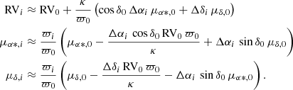
The PM and RVs of individual stars are affected by the projection effect due to the relative motion and position between the cluster and the Sun. Not correcting the projection artefacts could lead to false rotation and contraction signatures in nearby star clusters. The PM (μα * ,i, μδ * ,i) and RV (RVi) resulting from the projection effect of the cluster motion can be calculated as follows (van Leeuwen 2009):
 (1)
(1)
Here, RV0 is the cluster RV, ϖ0 is its parallax, ϖi is the stellar parallax, δ0 is the cluster declination, (μα * ,0, μδ, 0) is the cluster’s PM, (Δαi, Δδi) is the stellar angular separation from the cluster centre in radians, and κ is 4.74047 (the conversion factor for 1 mas yr−1 at 1 kpc to 1 km s−1).
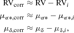
The PM (μα * ,corr, μδ, corr) and RV (RVcorr) corrected for the bulk cluster motion and projection effect are as follows:
 (2)
(2)
where RV is the stellar RV and (μα*, μδ) is the stellar PM.
2.4. Synthetic clusters
2.4.1. Demo clusters
We created demo clusters to visualise the various observational aspects of cluster spin and the effects of observational errors on these observables.
The simplest synthetic cluster is a solid body rotator with a token rotational frequency of 40 cycles per gigayear (cy Gyr−1). These synthetic clusters have stars distributed in a sphere where the positions follow random normal distributions with σ = 3 pc. The initial rotation axis was assumed to be along the Z direction, which could be changed later depending on the required inclination.
However, real stellar systems have differential rotation. Hence, we created realistic cylindrically-rotating clusters with the following velocity law (Lynden-Bell 1967; Lanzoni et al. 2018):
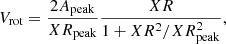 (3)
(3)
where XR is the projected distance measured from the spin axis, XRpeak corresponds to the rough radius up to which the cluster is virialised, and Apeak is the maximum amplitude of the RV. Typical Apeak values observed in globular clusters are 1–3 km s−1, while XRpeak values are 2–5 pc (Mackey et al. 2013; Kacharov et al. 2014; Lanzoni et al. 2018). Unfortunately, no such parameters were available for OCs; hence, we assumed that the Apeak of the demo clusters were similar to globular clusters. As some OCs may be virialised systems, we used two values of Rpeak: 2 pc for an unvirialised cluster and 10 pc for a virialised cluster. Rpeak of 2 pc is based on globular clusters and is useful to demonstrate the rotation curve of a partially virialised cluster. Rpeak of 10 pc means most of the OC is virialised and the rotation curve can be approximated to a linear trend (see bottom row of Fig. 1).
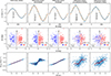 |
Fig. 1. Spin detection using RV. All these clusters have 90° inclination. First row: variation of ΔV across various PA. The fitted sin curve is shown in orange, while the grey bar shows the PApeak. Second row: spatial positions (Δl,Δb) of the stars coloured according to their RV. The identified spin axis (corresponding to PApeak) is shown in grey. Third row: variation of RVcorr with XR. The red curve shows the rolling average of the RVcorr values. |
Optionally, we can also add noise in the data to simulate the observables as seen through the Gaia telescope. The details of the used synthetic clusters and the added noise are given in Table A.1.
2.4.2. N-body simulated clusters
The demo clusters are non-physical due to the artificial assignment of velocities and positions. Hence, we also selected the following variety of N-body simulations to understand the presence of spin in realistic clusters.
– Kroupa+2022: We used archival N-body simulations of star clusters from Kroupa et al. (2022). They calculated the dynamical evolution of a grid of star clusters with total initial masses ranging from 2500 M⊙ to 20 000 M⊙ with 0.1 M⊙ stellar particles on a circular orbit with a Galactocentric distance of 8.3 kpc using the PHANTOM OF RAMSES code (Lüghausen et al. 2015). In this code, sub-routines were added to the RAMSES code (Teyssier 2002) in order to solve the MoNDian gravitational field equation in the QUMOND formulation (Milgrom 2010). As a collisionless field method requires a sufficient particle density in order to calculate a reliable potential, the 2500 M⊙ mass model already shows artificial effects of limited resolution.
– PETAR: We simulated clusters with 5000 particles in Newtonian dynamics using the direct N-body code PETAR (Wang et al. 2020). We created two simulations, the first with no primordial binaries and the second with 100% primordial binaries. For both models, the initial mass spectra were sampled from the Kroupa (2001) canonical initial mass function using the Plummer model with a half-mass radius of rh = 3 pc. We employed the Milky Way potential as an external field (Bovy 2015). Both demo clusters were located 8 kpc from the Galactic centre and have a circular orbit along the disc. We also enable stellar evolution using the updated SSE/BSE code (Hurley et al. 2000, 2002; Banerjee et al. 2020), which is embedded in PETAR. The remnant mass is based on the rapid supernovae scenario from Fryer et al. (2012). The calculation also includes the pair-instability (Belczynski et al. 2016) and electron capture supernova (Belczynski et al. 2008). We assume a solar metallicity Z = 0.02 for both models (von Steiger & Zurbuchen 2016). Table 1 lists the relevant stellar evolution parameters and the used values for both calculations.
Relevant SSE/BSE parameters for simulations with PETAR.
– Milgromian Law Dynamics (MLD): As QUMOND (Milgrom 2010) and AQUAL (Bekenstein & Milgrom 1984) are non-linear field-theoretical formulations of MoND, stellar dynamical codes for the evolution of discrete systems are very difficult to construct and currently not available. As a first step, the standard Hermite scheme is extended to solve Milgrom’s law (Milgrom 1983) for a discrete N-body system (Pflamm-Altenburg 2024). The MLD code includes smoothing of the inter-particle forces in the Newtonian regime in order to suppress Newtonisation of centre-of-mass motions of close compact sub-systems. We simulated a Hyades-like cluster with 2000 particles with 0.5 M⊙ each. This stellar system of 2000 particles requires a direct N-body solver because simulations performed with a particle-mesh code (e.g., PoR) would be strongly affected by resolution limitations.
The six-dimensional astrometry (α, δ, ϖ, μα, μδ, RV) of the synthetic clusters was then used to perform synthetic observations and create diagnostic plots similar to real OCs as mentioned in Sect. 3. To avoid the contamination from tidal tails along the line of sight, we kept the position of the observer (Sun) along the line connecting the cluster centre to the Galactic centre. The overall results do not change if we use the corotating reference frame instead of the inertial frame.
2.5. Spin detection using radial velocity
As the Galactic potential in the solar neighbourhood is approximately axisymmetric around the Galactic Z axis, we use the Galactic coordinates (l, b) as the base coordinates for this particular step2. First, we projected the cluster on a tangential plane and measured relative Galactic coordinates (Δl, Δb). Then, we divided the cluster into two sectors for an arbitrary position angle (PA; as measured clockwise from the Galactic east direction, in the sky plane). The difference between the mean RV of the two halves (ΔV) will increase if the assumed PA is along the spin axis. We shifted the PA from 0° to 360° in steps of 15°. The PA–ΔV distribution was then fitted with a sin wave, which gives the PApeak with maximum ΔV and the ΔV amplitude (≈ twice the velocity dispersion).
We used the same process to measure the best-fit PA for different annuli. A rotating cluster should have similar PA for the whole cluster and the different annuli. The central region contains the noisiest data due to relatively higher velocity dispersion compared to the differential RV. Hence, we removed the central 25th percentile data for our final classification to bring out the rotation signature. To further analyse the cluster, we created a new coordinate system (XR,YR) where YR was along the PA vector, while XR was perpendicular to it.
The first row in Fig. 1 shows examples of the PA–ΔV plots for synthetic clusters. All the demo clusters have the rotation axis along the Galactocetric Z axis (parallel to b). The maximum of the sin curve gives PApeak, shown as an arrow in the second row, along with the RV distribution along the sky. The third row shows the resulting XR–RVcorr variation. This relation is linear for a solid body rotator and roughly linear for a virialised cluster. The last two columns of Fig. 1 show the effect of adding noise to the data due to internal velocity dispersion and Gaia-like observational errors. The observed XR–RVcorr curves in these noisy demo clusters only retain a rough increasing trend, where the differences due to possible virialisation are hidden due to the noise.
2.6. Spin detection using proper motion
Figure 2 shows the views of rotating clusters as seen along the spin axis. The tangential components of PM (μT) contain the rotation signature of the cluster. The μT will increase with projected radius (R) if the cluster rotates (assuming the spin axis is along the line of sight).
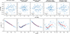 |
Fig. 2. Spin detection using PM. All these clusters have 0° inclination. First row: spatial positions (Δα,Δβ) of the stars, along with the arrows indicating the PM of each star. Second row: variation of μT with radius. The red curve shows the rolling average of the μT values. |
In an ideal case with a solid body rotation, one expects a linear distribution in the μT and R as seen in the first column of Fig. 2. However, in the case of a differential rotator, the rotation speed varies across the radius. Thus, one would expect an increase in μT until R ≈ Rpeak and then a slight dip. However, as shown by the last column of Fig. 2, a virialised OC should have a linear trend in the R–μT plot.
2.7. Expansion or contraction using proper motion
The radial component of PM (μR) shows the radial motion of the stars. The μR should not change with radius in a stable cluster. However, in an expanding cluster, μR will increase with the radius, and in a contracting cluster, μR will decrease with the radius. To identify the possible expansion or contraction, we created an R–μR plot for each cluster. The slope of the R–μR distribution gives the expansion rate of the cluster.
2.8. Cluster orbits
We used the cluster position and motion to calculate the cluster’s orbit around the Milky Way using ASTROPY (Astropy Collaboration 2013, 2018, 2022) and GALPY (Bovy 2015). We assumed the MWPotential2014 Milky Way potential, solar position (−8000, 0, 15 pc), and velocity (10, 235, 7 km s−1) (Bovy 2015). The cluster orbits plotted in diagnostic plots are of arbitrary time used for analytical assistance.
2.9. Statistical tests and effect of observational errors
The XR–RVcorr, R–μT, and R–μR distributions were fitted with a linear function to calculate the RV-based rotation, PM-based rotation, and expansion, respectively. Before fitting the line, we removed the 3σ outliers. The observational uncertainties in astrometric parameters were propagated while measuring the slope and its uncertainty. The possible covariances between the astrometric parameters were ignored. The measurement of PA requires averaged velocities of two halves of the cluster. The uncertainties used while finding the PApeak are Poissonian in nature based on the number of stars in each half (roughly > 50 stars for the half-cluster and > 12 for each radial half-slice mentioned in Sect. 2.5 and Fig. A.1). These Poisson errors were used while fitting the sin curve and the uncertainty in the PApeak.
The RV analysis gives the XR–RVcorr distribution. We performed the KS test to check whether the two populations in the two halves of the cluster were significantly different (p < 0.05). We also fitted a line to this distribution, the slope of which gives the ν cos i component of the spin axis in an ideal solid body rotation. The line fitting included outlier rejection and accounted for parameter uncertainties. We consider the ν cos i measurement to be statistically significant if it passes the KS test and the fitted measurement of ν cos i was better than 1σ.
For the PM analysis, a Spearman rank-order correlation test was applied to the R–μT distribution to identify any monotonicity. Due to the noisy data, we used a Monte Carlo approach to create multiple realisations with values shifted with a Gaussian noise proportional to the errors. The median statistic (≥0.4) and p (≤0.05) of the resulting Spearman tests were used to identify monotonic trends in the distributions. The slope of the R–μT plot gives the value of ν sin i for a solid body rotator. We considered the ν sin i measurement to be statistically significant if it passes the Spearman test and the fitted measurement of ν cos i was better than 1σ.
The noisy Spearman rank-order correlation test was also applied to the R–μR plots to identify monotonicity. We considered the expansion rate measurement to be statistically significant if it passed the Spearman test and the fitted slope measurement was better than 1σ.
Figure 3 shows the effect of observational errors on the measurements of ν cos i and ν sin i in a solid body rotator. The markers are also filled according to their statistical significance. The figure shows that most of the ν cos i or ν sin i measurements lie within 1σ of the original value. The low inclination systems show measurable and significant ν cos i values, which could be overestimated in the presence of noise. The high-inclination systems show measurable and significant PM ν sin i values, which could be overestimated in the presence of noise. Overall, the RV method (top panel in Fig. 3) is more noise resistant than the PM method (bottom panel in Fig. 3).
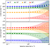 |
Fig. 3. Effect of observed velocity error on measurement of ν cos i and ν sin i on a solid body rotator with ν = 100 cy Gyr−1. The statistically significant results (see Sect. 2.9) are represented by filled circles, and the corresponding 1σ errors are shown in the shaded areas. The horizontal lines show the measurements with no error. The typical errors in Gaia RV (1.3 km s−1) and PM (0.02 km s−1) are shown as dashed grey lines. |
3. Results
3.1. Open clusters using Gaia data
Observationally, the inclination of the cluster’s orbit is not known. Hence, we created diagnostic plots to identify spin signatures using both RV and PM. Figure 4 shows an example of such a diagnostic plot. Here, spatial plots show the variation of RV and PM across the cluster members. The R–μT and XR–RVcorr plots are the primary indicators of the spin. The polar plot shows the values of identified PA using different radial slices of the cluster (as shown in Fig. A.1). Ideally, all the PA values should be similar. We have removed the central 25th percentile stars while analysing the RVs to avoid the noisy velocities near the cluster centre. Including the central stars increases the errors of the parameters; however, this does not change the overall results for the gold sample defined later.
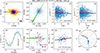 |
Fig. 4. Diagnostic plots for NGC 2099. (a) Spatial distribution of cluster members and candidates. The stars are coloured according to the membership probability. (b) The spatial distribution of stars along with arrows indicating their PM. (c) Variation of μT with radius. (d) Variation of μR with radius. (e) Variation of ΔV with PA. The PApeak is shown as a grey band, and the fitted sin curve is orange. (f) Spatial distribution of stars coloured according to RVcorr. The orbital axis corresponding to PApeak is shown as the grey arrow. (g) Distribution of RVcorr with XR. (h) Variation of PApeak for different radial slices of the cluster. The radial distance used here is the average radius of the stars within the selection, and the radial error bars show the minimum–maximum radius within the radial slice. The green wedge points towards the cluster’s orbital motion in (a), (b), and (f). The red curves show the rolling average in (c), (d), and (g). The black lines show the linear fits in (c), (d), and (g). The core radii (grey solid circle or line) and tidal radii (grey dashed circle or line) are shown in (a), (b), and (c). |
As seen in Figs. 1 and 2, a virialised cluster produces linear trends in the XR–RVcorr and R–μT plots. The two-body relaxation time for OCs ranges from a few megayears to a gigayear (Jadhav & Subramaniam 2021). The distribution in the R–μT and XR–RVcorr plots vary with different stages of relaxation and tend towards linearity for virialised clusters. We have fitted these distributions with lines to gauge the extent of the spin. The slope of the XR–RVcorr data gives ν cos i in ideal conditions, while the slope of the R–μT data gives the ν sin i. However, the noise and state of relaxation change the slope values. We report the values of the slopes in Table 2. However, it has to be noted that the values are rough estimates of the real spin frequency, and the quoted errors are formal errors based on line fitting (without accounting for virialisation or internal velocity dispersion). The individual diagnostic plots for the spinning clusters using the RV and PM methods are given in Figs. A.3 and A.4, respectively. The diagnostic plots for expanding and contracting clusters are given in Figs. A.5 and A.6, respectively.
Properties of spinning clusters.
Overall, we identified 22 clusters with some indication of rotation using RV-based analysis. Six of the clusters passed the KS test and > 1σ slope significance test (see Sect. 2.9) and are referred to as the ‘RV-based gold sample’. Ten of these clusters passed at least one of the tests and are classified in the RV-based silver sample. The remaining six clusters did not show any significant trends in the Gaia DR3 + SoS data; however, they did show significant trends in the SoS-only analysis. These clusters are also classified as part of the RV-based silver sample, and the use of SoS-only data is mentioned in the corresponding tables and figures. The PM analysis showed spin signatures in four OCs (referred to as ‘PM-based gold sample’). The μR analysis identified 18 expanding clusters and the contacting clusters.
3.2. N-body simulations
We analysed the evolution of cluster properties (angular momentum, ν cos i, radius) for the various N-body simulations. Figure A.2 shows their evolution in the simulated clusters. All the clusters revolve clockwise about the Galaxy, as seen from the Galactic north pole. Thus, their orbital angular momentum in the Z direction, as measured from the Galactic centre, was negative. We calculated the spin angular momentum (ℒz) in the co-rotating reference frame, assuming the centre of density as the origin. The evolution of ℒz is shown in the second row of Fig. A.2. In order to identify the cluster members, we calculated the kinetic and potential energies of the simulated particles with CLUSTERTOOLS (Webb 2023) using the positions and velocities of individual particles. Similarly, we measured the tidal radius based on the Galactic potential (Bovy 2015) and Bertin & Varri (2008) formalism. The ℒz is plotted for three populations: (i) stars within the tidal radius; (ii) bound stars, which have negative total energy (kinetic+potential); (iii) unbound stars, which have positive total energy. The stars within the tidal radius best represent the observed cluster members for real clusters.
The angular momentum of the whole system changes with time due to escaping particles, stellar evolution, and external forces. However, all simulations show significantly negative ℒz for unbound particles (i.e., the tidal tails), indicating that the spin axis of the tidal tail particles is aligned with the revolution axis. The stars within the tidal radius collectively do not have much angular momentum. However, the sign of this minimal ℒz is almost always negative. The only exceptions were the very early stages of the simulations.
The synthetic observations of these simulations provide the PA and ν cos i values for each snapshot. The PETAR simulations show that the cluster members predominantly rotate with their spin axis aligned with the revolution axis. Seven out of eight snapshots in MLD simulations do not show any rotation. The Kroupa+2022 clusters seem to have some rotation signatures; however, their spin axis alignment keeps fluctuating.
In addition, the spin was much stronger for bound stars. The bound stars span a larger radius, and the outer bound stars are not considered cluster members from an observational perspective. However, the ℒz and ν cos i measurements were much more significant for this collection. The bound stars mostly form a spinning population after ≈25 Myr in almost all simulations. Moreover, the majority of the time, the spin axis was aligned with the orbital angular momentum.
Overall, some simulated clusters have a detectable spin with ν cos i ranging from −2 to 2 cy Gyr−1. However, the spin orientation was not always aligned with the orbital angular momentum. Additionally, none of the simulated clusters showed statistically significant expansion signatures within the tidal radius of individual snapshots.
4. Discussion
4.1. Cluster expansion or contraction
Table 3 provides the expansion rates for the expanding and contracting clusters. Figure 5 shows the variation of the expansion rate with the cluster properties. 18 clusters younger than 100 Myr show expansion signatures (3.6% of the 492 OCs with similar ages). Panel a shows that the expansion rate decreases with age, becoming negative near 100–300 Myr. None of the older clusters showed detectable expansion or contraction. The theoretical expansion rate of the 40% Lagrangian radius (Kroupa et al. 2001) closely matches the observed expansion rate. No relation was found with the Galactocentric radius or the number of stars in the clusters. However, it is important to note that not all young clusters showed expansion.
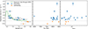 |
Fig. 5. Relations between cluster expansion rate and cluster properties such as the age, Galactocentric distance (RGC), and number of stars in the cluster (Nstars). The first panel shows the expansion rate (in green) of the 40% Lagrangian radius in an 8340 M⊙ cluster N-body model that undergoes gas expulsion and mass loss through evolving stars and reproduces the Orion Nebula Cluster at 1 Myr and the Pleiades cluster at 100 Myr. |
Properties of expanding or contracting (negative expansion rate) clusters.
4.2. Cluster spin
Figure 6 depicts the relation between the cluster properties and their spin. Panel a shows the cluster orbits and spin axis orientation with respect to the Galactic plane. All clusters are orbiting the Galactic centre clockwise (as seen from the North Pole with the Sun at −8 kpc). However, there is no correlation between the spin axis of the clusters and the Z direction. Panels b–d show the distribution of spin frequency with the cluster’s age, Galactocentric distance and the number of members within the tidal radius. There was no significant trend seen in all three distributions. The overall value of ν cos i ranges from 2–170 cy Gyr−1 and ν sin i are all around 15 cy Gyr−1. The analysis of our demo clusters showed that measurement of both ν sin i and ν sin i is possible in non-noisy clusters and can be reliably used to calculate the inclination and the true spin frequency. However, as real clusters are not perfect rotators and none of the observed clusters showed rotation signatures in both RV and PM methods, we cannot calculate the true frequency of the observed clusters.
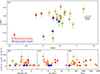 |
Fig. 6. Diagnostic plots for analysing relation between spin orientation and cluster properties. The RV-based gold sample, RV-based silver sample, and PM-based sample are shown by red, orange, and blue markers, respectively. A spin axis going into and coming out of the plane is shown as ⊗ and ⊙, respectively. (a) Galactocentric positions of clusters as seen from the Galactic north pole. The cluster orbits are shown in light green, and the Sun’s position is represented by the black cross. (b) Distribution of spin frequency with the cluster age. The RV-based method gives the ν cos i component of the spin frequency (ν), while the PM-based method gives the ν sin i component. (c) Distribution of spin frequency with the Galactocentric radius. (d) Distribution of spin frequency with the number of cluster members within the tidal radius with robust distance measurements. |
The simulated clusters showed minimal spin frequencies (−2 to 2 cy Gyr−1), mostly aligned with the orbital angular momentum. This slight spin could be due to the asymmetric evaporation of stars as seen by Kroupa et al. (2022) who noticed that the leading tail was more dense than the trailing tail. However, the observed clusters have much higher spin frequencies (ν cos igoldsample ∈ [ − 84, 30], ν cos isilversample ∈ [ − 77, 167] and ν sin i ∈ [ − 16, 13] cy Gyr−1).
The simulated clusters were set up without any spin. Hence, the result shows that the cluster spin due to internal dynamics and interaction with a smooth Galactic potential is minimal. Thus, primordial spin within the parent molecular cloud or a significantly strong dynamical interaction (such as collisions, flybys, and/or mergers of clusters) is required to explain the detected spin frequencies (up to 170 cy Gyr−1).
According to Braine et al. (2020), the RV gradient for molecular clouds in the galaxy M 51 goes up to 0.2 km s−1 pc−1 (equivalent to ν cos i ≤ 32 cy Gyr−1). This is consistent with the spin frequencies observed in the OCs. The initial spin would also explain the age independence of spin frequency and the randomness of the PA.
Toomre & Toomre (1972), Read et al. (2006), and Kroupa et al. (2022) have shown that stars in prograde orbits within a stellar system are preferentially lost compared to stars in retrograde orbits. This could have been interpreted as losing prograde angular momentum resulting in a star system spinning in the opposite direction to its orbit. However, the N-body simulations in this work showed that the cluster’s spin was majorly aligned with the orbital angular momentum. Additionally, the observations showed that the spin does not correlate with the orbital angular momentum, which is likely a result of external effects such as interactions or initial spin.
All the N-body simulations used in this study assume that the Galactic potential is axisymmetric. However, the presence of bar and spiral arms changes the Galactic potential and their rotation makes the potential evolve with time. Rossi & Hurley (2015) demonstrated that the Galactic bar has negligible effect on the cluster evolution for Galactocentric distance of more than 4 kpc. As all of the peculiar clusters in this study lie well beyond 6 kpc, the effect of Galactic bar should be minimal. However, more detailed simulations including a bar, spiral arms, primordial spin, and collisions with star clusters or molecular clouds would be helpful to further study the present-day spins seen in the OCs.
4.3. Comparison with literature on open clusters
Kamann et al. (2019) detected rotation in NGC 6791 and the absence of rotation in NGC 6819 using an RV-based analysis. We were not able to detect rotation in either of the clusters. Healy & McCullough (2020) detected signs of contraction in NGC 2516; however, we cannot confirm any radial motion in the cluster. Loktin & Popov (2020) used Gaia DR2 data and detected rotation in Praesepe. However, they did not correct for the projection effect which leads to erroneous results. Healy et al. (2021) detected rotation in Praesepe and the absence of rotation in Pleiades and M 35 (NGC 2168). Similarly, Hao et al. (2022, 2024) detected rotation in Praesepe, Pleiades, Alpha Persei, and Hyades. Our analysis, after correcting for the projection effects, shows a slight rotation signature in Praesepe (NGC 2632) and Alpha Persei (Melotte 20). However, we did not detect any rotation in the Pleiades (Melotte 22), Hyades (Melotte 25), and NGC 2168. Guilherme-Garcia et al. (2023) used a PM-based analysis to identify eight spinning (and 9 candidates), 14 expanding (and 15 candidates), and two contracting (and 1 candidate) clusters. They used vector field reconstruction to identify kinematic structures in R–μT and R–μR plots. However, they did not quantify the spin or expansion rates. We have two of the spinning clusters in our sample (Ruprecht 147 and Stock 2). In addition, one of their spinning clusters, Alessi 13, had a significant slope in the R–μT plane; however, it did not pass the Spearman test for monotonicity. Among their 14 expanding clusters, two are common with our list (Alessi 13 and Collinder 69). The differences in the classification method and in the parent sample led to the differences in the list of clusters.
5. Conclusions
We analysed the internal dynamics of OCs using Gaia DR3 data, specifically the spin and expansion of the clusters. We also used synthetic observations of N-body simulations to validate the results. The major conclusions of the work are as follows.
-
Among the 1379 OCs identified with Gaia DR3, we were able to detect spin signatures in ten (0.7%) clusters with 16 more candidate OCs. The spin frequencies are roughly 9–167 cy Gyr−1. Of these 26, 12 spin in the same direction as they orbit the Galaxy.
-
The N-body simulations of similar clusters have a spin frequency of ≈2–5 cy Gyr−1.
-
The observed spin frequencies are much larger than expected for initially non-rotating clusters. Thus, we conclude that their parent molecular clouds must have initial spin, and/or the clusters have undergone strong tidal interactions with other massive objects in the Milky Way.
-
The spin orientation in N-body simulations majorly aligns with the cluster’s orbit, contrary to previous conjectures based on preferential tidal stripping of stars with prograde orbits. Observationally, the spin orientation is not correlated with the orbital angular momentum. Any spin imparted due to the tidal stripping is dominated by random sources of spin (such as initial spin and interactions).
-
From the same sample, we were able to identify 18 (3.6% of the OCs younger than 100 Myr) expanding and three contracting clusters. The expansion rate of these young clusters is compatible with theoretical models of cluster expansion due to gas expulsion, stellar mass loss, and dynamical heating.
The RV and parallax precision are the major hurdles in identifying more spinning or expanding OCs. Recent attempts, such as the SoS, are improving the RV homogeneity and precision using multiple spectroscopic surveys. Upcoming spectroscopic surveys with better precision and fainter stars would be necessary for the understanding of the 3D dynamics of the OCs. In addition, simulations with primordial spin and external interactions would be required to understand the spinning nature and origin of OCs thoroughly.
The method used to detect rotation in Praesepe is erroneous and is affected by the projection effects due to the solar motion.
The 0 1 difference between the Galactic midplane and the b = 0 plane does not affect the results of this study.
Acknowledgments
We thank the anonymous referee for constructive comments. VJ thanks the Alexander von Humboldt Foundation for their support. PK acknowledges support through the DAAD Eastern European Exchange Programme. This work has made use of data from the European Space Agency (ESA) mission Gaia (https://www.cosmos.esa.int/gaia), processed by the Gaia Data Processing and Analysis Consortium (DPAC, https://www.cosmos.esa.int/web/gaia/dpac/consortium). Funding for the DPAC has been provided by national institutions, in particular the institutions participating in the Gaia Multilateral Agreement.
References
- Ahumada, R., Allende Prieto, C., Almeida, A., et al. 2020, ApJS, 249, 3 [NASA ADS] [CrossRef] [Google Scholar]
- Anderson, J., & King, I. R. 2003, AJ, 126, 772 [NASA ADS] [CrossRef] [Google Scholar]
- Astropy Collaboration (Robitaille, T. P., et al.) 2013, A&A, 558, A33 [NASA ADS] [CrossRef] [EDP Sciences] [Google Scholar]
- Astropy Collaboration (Price-Whelan, A. M., et al.) 2018, AJ, 156, 123 [Google Scholar]
- Astropy Collaboration (Price-Whelan, A. M., et al.) 2022, ApJ, 935, 167 [NASA ADS] [CrossRef] [Google Scholar]
- Bailer-Jones, C. A. L., Rybizki, J., Fouesneau, M., Demleitner, M., & Andrae, R. 2021, AJ, 161, 147 [Google Scholar]
- Banerjee, S., Belczynski, K., Fryer, C. L., et al. 2020, A&A, 639, A41 [NASA ADS] [CrossRef] [EDP Sciences] [Google Scholar]
- Bekenstein, J., & Milgrom, M. 1984, ApJ, 286, 7 [NASA ADS] [CrossRef] [Google Scholar]
- Belczynski, K., Kalogera, V., Rasio, F. A., et al. 2008, ApJS, 174, 223 [Google Scholar]
- Belczynski, K., Heger, A., Gladysz, W., et al. 2016, A&A, 594, A97 [NASA ADS] [CrossRef] [EDP Sciences] [Google Scholar]
- Bellini, A., Bianchini, P., Varri, A. L., et al. 2017, ApJ, 844, 167 [NASA ADS] [CrossRef] [Google Scholar]
- Bertin, G., & Varri, A. L. 2008, ApJ, 689, 1005 [NASA ADS] [CrossRef] [Google Scholar]
- Bianchini, P., van der Marel, R. P., del Pino, A., et al. 2018, MNRAS, 481, 2125 [Google Scholar]
- Bovy, J. 2015, ApJS, 216, 29 [NASA ADS] [CrossRef] [Google Scholar]
- Braine, J., Hughes, A., Rosolowsky, E., et al. 2020, A&A, 633, A17 [NASA ADS] [CrossRef] [EDP Sciences] [Google Scholar]
- Chen, H. H.-H., Pineda, J. E., Offner, S. S. R., et al. 2019, ApJ, 886, 119 [Google Scholar]
- Choudhuri, A. R. 2010, Astrophysics for Physicists (Cambridge: Cambridge University Press) [CrossRef] [Google Scholar]
- Deng, L.-C., Newberg, H. J., Liu, C., et al. 2012, RAA, 12, 735 [Google Scholar]
- Dinnbier, F., & Kroupa, P. 2020a, A&A, 640, A84 [EDP Sciences] [Google Scholar]
- Dinnbier, F., & Kroupa, P. 2020b, A&A, 640, A85 [EDP Sciences] [Google Scholar]
- Dinnbier, F., Kroupa, P., & Anderson, R. I. 2022, A&A, 660, A61 [NASA ADS] [CrossRef] [EDP Sciences] [Google Scholar]
- Fabricius, C., Luri, X., Arenou, F., et al. 2021, A&A, 649, A5 [NASA ADS] [CrossRef] [EDP Sciences] [Google Scholar]
- Fryer, C. L., Belczynski, K., Wiktorowicz, G., et al. 2012, ApJ, 749, 91 [Google Scholar]
- Gaia Collaboration (Prusti, T., et al.) 2016, A&A, 595, A1 [NASA ADS] [CrossRef] [EDP Sciences] [Google Scholar]
- Gaia Collaboration (Brown, A. G. A., et al.) 2018, A&A, 616, A1 [NASA ADS] [CrossRef] [EDP Sciences] [Google Scholar]
- Gaia Collaboration (Brown, A. G. A., et al.) 2021, A&A, 649, A1 [NASA ADS] [CrossRef] [EDP Sciences] [Google Scholar]
- Gaia Collaboration (Vallenari, A., et al.) 2023, A&A, 674, A1 [NASA ADS] [CrossRef] [EDP Sciences] [Google Scholar]
- Gilmore, G., Randich, S., Asplund, M., et al. 2012, The Messenger, 147, 25 [NASA ADS] [Google Scholar]
- Guilherme-Garcia, P., Krone-Martins, A., & Moitinho, A. 2023, A&A, 673, A128 [NASA ADS] [CrossRef] [EDP Sciences] [Google Scholar]
- Hao, C. J., Xu, Y., Bian, S. B., et al. 2022, ApJ, 938, 100 [NASA ADS] [CrossRef] [Google Scholar]
- Hao, C. J., Xu, Y., Hou, L. G., et al. 2024, ApJ, 963, 153 [NASA ADS] [CrossRef] [Google Scholar]
- Healy, B. F., & McCullough, P. R. 2020, ApJ, 903, 99 [NASA ADS] [CrossRef] [Google Scholar]
- Healy, B. F., McCullough, P. R., & Schlaufman, K. C. 2021, ApJ, 923, 23 [NASA ADS] [CrossRef] [Google Scholar]
- Hénault-Brunet, V., Gieles, M., Evans, C. J., et al. 2012, A&A, 545, L1 [NASA ADS] [CrossRef] [EDP Sciences] [Google Scholar]
- Hobbs, G., Lorimer, D. R., Lyne, A. G., & Kramer, M. 2005, MNRAS, 360, 974 [Google Scholar]
- Hunt, E. L., & Reffert, S. 2023, A&A, 673, A114 [NASA ADS] [CrossRef] [EDP Sciences] [Google Scholar]
- Hurley, J. R., Pols, O. R., & Tout, C. A. 2000, MNRAS, 315, 543 [Google Scholar]
- Hurley, J. R., Tout, C. A., & Pols, O. R. 2002, MNRAS, 329, 897 [Google Scholar]
- Jadhav, V. V., & Subramaniam, A. 2021, MNRAS, 507, 1699 [NASA ADS] [CrossRef] [Google Scholar]
- Jerabkova, T., Boffin, H. M. J., Beccari, G., et al. 2021, A&A, 647, A137 [NASA ADS] [CrossRef] [EDP Sciences] [Google Scholar]
- Kacharov, N., Bianchini, P., Koch, A., et al. 2014, A&A, 567, A69 [NASA ADS] [CrossRef] [EDP Sciences] [Google Scholar]
- Kamann, S., Husser, T. O., Dreizler, S., et al. 2018, MNRAS, 473, 5591 [NASA ADS] [CrossRef] [Google Scholar]
- Kamann, S., Bastian, N. J., Gieles, M., Balbinot, E., & Hénault-Brunet, V. 2019, MNRAS, 483, 2197 [NASA ADS] [CrossRef] [Google Scholar]
- Kroupa, P. 1995a, MNRAS, 277, 1491 [Google Scholar]
- Kroupa, P. 1995b, MNRAS, 277, 1507 [NASA ADS] [Google Scholar]
- Kroupa, P. 2001, MNRAS, 322, 231 [NASA ADS] [CrossRef] [Google Scholar]
- Kroupa, P., Aarseth, S., & Hurley, J. 2001, MNRAS, 321, 699 [NASA ADS] [CrossRef] [Google Scholar]
- Kroupa, P., Jerabkova, T., Thies, I., et al. 2022, MNRAS, 517, 3613 [CrossRef] [Google Scholar]
- Kuhn, M. A., Hillenbrand, L. A., Sills, A., Feigelson, E. D., & Getman, K. V. 2019, ApJ, 870, 32 [CrossRef] [Google Scholar]
- Kutner, M. L., Tucker, K. D., Chin, G., & Thaddeus, P. 1977, ApJ, 215, 521 [NASA ADS] [CrossRef] [Google Scholar]
- Lada, C. J., & Lada, E. A. 2003, ARA&A, 41, 57 [Google Scholar]
- Lanzoni, B., Ferraro, F. R., Mucciarelli, A., et al. 2018, ApJ, 861, 16 [NASA ADS] [CrossRef] [Google Scholar]
- Loktin, A. V., & Popov, A. A. 2020, Astron. Nachr., 341, 638 [NASA ADS] [CrossRef] [Google Scholar]
- Lüghausen, F., Famaey, B., & Kroupa, P. 2015, Can. J. Phys., 93, 232 [CrossRef] [Google Scholar]
- Lynden-Bell, D. 1967, MNRAS, 136, 101 [Google Scholar]
- Mackey, A. D., Da Costa, G. S., Ferguson, A. M. N., & Yong, D. 2013, ApJ, 762, 65 [CrossRef] [Google Scholar]
- Milgrom, M. 1983, ApJ, 270, 365 [Google Scholar]
- Milgrom, M. 2010, MNRAS, 403, 886 [NASA ADS] [CrossRef] [Google Scholar]
- Moreno, E., Pichardo, B., & Velázquez, H. 2014, ApJ, 793, 110 [Google Scholar]
- Moreno, E., Fernández-Trincado, J. G., Schuster, W. J., Pérez-Villegas, A., & Chaves-Velasquez, L. 2021, MNRAS, 506, 4687 [CrossRef] [Google Scholar]
- Moreno, E., Fernández-Trincado, J. G., Pérez-Villegas, A., Chaves-Velasquez, L., & Schuster, W. J. 2022, MNRAS, 510, 5945 [NASA ADS] [CrossRef] [Google Scholar]
- Pfalzner, S., & Kaczmarek, T. 2013, A&A, 559, A38 [NASA ADS] [CrossRef] [EDP Sciences] [Google Scholar]
- Pflamm-Altenburg, J. 2024, A&A, submitted [Google Scholar]
- Piatti, A. E., & Malhan, K. 2022, MNRAS, 511, L1 [NASA ADS] [CrossRef] [Google Scholar]
- Read, J. I., Wilkinson, M. I., Evans, N. W., Gilmore, G., & Kleyna, J. T. 2006, MNRAS, 366, 429 [NASA ADS] [CrossRef] [Google Scholar]
- Rosolowsky, E., Engargiola, G., Plambeck, R., & Blitz, L. 2003, ApJ, 599, 258 [NASA ADS] [CrossRef] [Google Scholar]
- Rossi, L. J., & Hurley, J. R. 2015, MNRAS, 454, 1453 [NASA ADS] [CrossRef] [Google Scholar]
- Sollima, A., Baumgardt, H., & Hilker, M. 2019, MNRAS, 485, 1460 [Google Scholar]
- Steinmetz, M., Matijevič, G., Enke, H., et al. 2020, AJ, 160, 82 [NASA ADS] [CrossRef] [Google Scholar]
- Szigeti, L., Mészáros, S., Szabó, G. M., et al. 2021, MNRAS, 504, 1144 [NASA ADS] [CrossRef] [Google Scholar]
- Teyssier, R. 2002, A&A, 385, 337 [CrossRef] [EDP Sciences] [Google Scholar]
- Toomre, A., & Toomre, J. 1972, ApJ, 178, 623 [Google Scholar]
- Tsantaki, M., Pancino, E., Marrese, P., et al. 2022, A&A, 659, A95 [NASA ADS] [CrossRef] [EDP Sciences] [Google Scholar]
- Tutukov, A. V. 1978, A&A, 70, 57 [NASA ADS] [Google Scholar]
- van de Ven, G., van den Bosch, R. C. E., Verolme, E. K., & de Zeeuw, P. T. 2006, A&A, 445, 513 [NASA ADS] [CrossRef] [EDP Sciences] [Google Scholar]
- van Leeuwen, F. 2009, A&A, 497, 209 [CrossRef] [EDP Sciences] [Google Scholar]
- Vasiliev, E., & Baumgardt, H. 2021, MNRAS, 505, 5978 [NASA ADS] [CrossRef] [Google Scholar]
- von Steiger, R., & Zurbuchen, T. H. 2016, ApJ, 816, 13 [Google Scholar]
- Wang, L., Iwasawa, M., Nitadori, K., & Makino, J. 2020, MNRAS, 497, 536 [NASA ADS] [CrossRef] [Google Scholar]
- Webb, J. 2023, J. Open Source Softw., 8, 4483 [NASA ADS] [CrossRef] [Google Scholar]
- Zwitter, T., Kos, J., Chiavassa, A., et al. 2018, MNRAS, 481, 645 [NASA ADS] [CrossRef] [Google Scholar]
Appendix A: Supplementary table and figures
Cluster parameters of the synthetic demo clusters. The cluster position was fixed at (−8300,0,0) pc with zero velocity. The inclination (i) was measured from the line of sight. All rotation axes are in the Galactocentric XY plane. The velocity noise is composed of typical internal velocity dispersion in OCs (0.5 km s−1; Choudhuri 2010) and typical errors in the Gaia DR3 observations for a cluster at 300 pc (Gaia Collaboration 2021: RV_error ≈1.3 km s−1; Fabricius et al. 2021: PM_error ≈0.02 km s−1). The meanings of the suffixes are as follows: sb: solid body, dr: differential rotation, vir: virialised, unvir: non-virialised, n: noise included.
Definitions and formulae for various observed and calculated parameters in this work.
 |
Fig. A.1. Demonstration of various radial slices used while calculating the PA. The grey circles denote the radii of the circles within which the 25th, 50th, 75th, and 100th percentiles of the members reside. The 25th–100th percentile region is used for the RV-based analysis as it avoids the noisy velocities in the cluster centre. |
 |
Fig. A.2. Evolution of the properties of simulated clusters. First row: The evolution of the number of stars which are bound (orange), unbound (green) and are within the tidal radius (blue). Here, the bound and unbound means the sum of the kinetic and potential energy of the particle is negative and positive, respectively. The numbers are normalised with respect to the total population: 5000, 5000, 2000, 2000, 50000, and 50000 for the columns from left to right, respectively. Second row: Spin angular momentum in the centre of density frame (ℒz). The ℒz values are arbitrarily scaled for visual clarity. A negative value means the cluster is spinning in the same direction as it’s orbit i.e. orbital and spin vectors are aligned. The colours are the same as the first row. Third row: Core (black) and tidal (grey) radius. Fourth row: PA (90≡counter-rotation, 270≡aligned rotation). The PA measurement for bound stars is shown in olive, while the stars within the tidal radius are shown in red. Fifth row: Spin frequency, ν cos i, for the corresponding PA. |
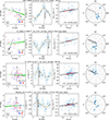 |
Fig. A.3. (Continued…). Diagnostic plots for RV-based spinning clusters. All the subplots are similar to those in Figure 4. |
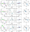 |
Fig. A.3. (Continued…). Diagnostic plots for RV-based spinning clusters. All the subplots are similar to those in Figure 4. |
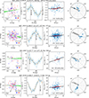 |
Fig. A.3. (Continued…). Diagnostic plots for RV-based spinning clusters. All the subplots are similar to those in Figure 4. |
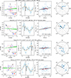 |
Fig. A.3. (Continued…). Diagnostic plots for RV-based spinning clusters. All the subplots are similar to those in Figure 4. |
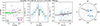 |
Fig. A.3. (Continued…). Diagnostic plots for RV-based spinning clusters. All the subplots are similar to those in Figure 4. |
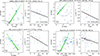 |
Fig. A.4. Diagnostic plots for PM-based spinning clusters. All the subplots are similar to those in Figure 4. |
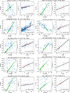 |
Fig. A.5. Diagnostic plots for expanding clusters. All the subplots are similar to those in Figure 4. |
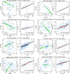 |
Fig. A.5. Continued. Diagnostic plots for expanding clusters. All the subplots are similar to those in Figure 4. |
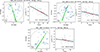 |
Fig. A.6. Diagnostic plots for contracting clusters. All the subplots are similar to those in Figure 4. |
All Tables
Cluster parameters of the synthetic demo clusters. The cluster position was fixed at (−8300,0,0) pc with zero velocity. The inclination (i) was measured from the line of sight. All rotation axes are in the Galactocentric XY plane. The velocity noise is composed of typical internal velocity dispersion in OCs (0.5 km s−1; Choudhuri 2010) and typical errors in the Gaia DR3 observations for a cluster at 300 pc (Gaia Collaboration 2021: RV_error ≈1.3 km s−1; Fabricius et al. 2021: PM_error ≈0.02 km s−1). The meanings of the suffixes are as follows: sb: solid body, dr: differential rotation, vir: virialised, unvir: non-virialised, n: noise included.
Definitions and formulae for various observed and calculated parameters in this work.
All Figures
|
Fig. 1. Spin detection using RV. All these clusters have 90° inclination. First row: variation of ΔV across various PA. The fitted sin curve is shown in orange, while the grey bar shows the PApeak. Second row: spatial positions (Δl,Δb) of the stars coloured according to their RV. The identified spin axis (corresponding to PApeak) is shown in grey. Third row: variation of RVcorr with XR. The red curve shows the rolling average of the RVcorr values. |
| In the text | |
|
Fig. 2. Spin detection using PM. All these clusters have 0° inclination. First row: spatial positions (Δα,Δβ) of the stars, along with the arrows indicating the PM of each star. Second row: variation of μT with radius. The red curve shows the rolling average of the μT values. |
| In the text | |
|
Fig. 3. Effect of observed velocity error on measurement of ν cos i and ν sin i on a solid body rotator with ν = 100 cy Gyr−1. The statistically significant results (see Sect. 2.9) are represented by filled circles, and the corresponding 1σ errors are shown in the shaded areas. The horizontal lines show the measurements with no error. The typical errors in Gaia RV (1.3 km s−1) and PM (0.02 km s−1) are shown as dashed grey lines. |
| In the text | |
|
Fig. 4. Diagnostic plots for NGC 2099. (a) Spatial distribution of cluster members and candidates. The stars are coloured according to the membership probability. (b) The spatial distribution of stars along with arrows indicating their PM. (c) Variation of μT with radius. (d) Variation of μR with radius. (e) Variation of ΔV with PA. The PApeak is shown as a grey band, and the fitted sin curve is orange. (f) Spatial distribution of stars coloured according to RVcorr. The orbital axis corresponding to PApeak is shown as the grey arrow. (g) Distribution of RVcorr with XR. (h) Variation of PApeak for different radial slices of the cluster. The radial distance used here is the average radius of the stars within the selection, and the radial error bars show the minimum–maximum radius within the radial slice. The green wedge points towards the cluster’s orbital motion in (a), (b), and (f). The red curves show the rolling average in (c), (d), and (g). The black lines show the linear fits in (c), (d), and (g). The core radii (grey solid circle or line) and tidal radii (grey dashed circle or line) are shown in (a), (b), and (c). |
| In the text | |
|
Fig. 5. Relations between cluster expansion rate and cluster properties such as the age, Galactocentric distance (RGC), and number of stars in the cluster (Nstars). The first panel shows the expansion rate (in green) of the 40% Lagrangian radius in an 8340 M⊙ cluster N-body model that undergoes gas expulsion and mass loss through evolving stars and reproduces the Orion Nebula Cluster at 1 Myr and the Pleiades cluster at 100 Myr. |
| In the text | |
|
Fig. 6. Diagnostic plots for analysing relation between spin orientation and cluster properties. The RV-based gold sample, RV-based silver sample, and PM-based sample are shown by red, orange, and blue markers, respectively. A spin axis going into and coming out of the plane is shown as ⊗ and ⊙, respectively. (a) Galactocentric positions of clusters as seen from the Galactic north pole. The cluster orbits are shown in light green, and the Sun’s position is represented by the black cross. (b) Distribution of spin frequency with the cluster age. The RV-based method gives the ν cos i component of the spin frequency (ν), while the PM-based method gives the ν sin i component. (c) Distribution of spin frequency with the Galactocentric radius. (d) Distribution of spin frequency with the number of cluster members within the tidal radius with robust distance measurements. |
| In the text | |
|
Fig. A.1. Demonstration of various radial slices used while calculating the PA. The grey circles denote the radii of the circles within which the 25th, 50th, 75th, and 100th percentiles of the members reside. The 25th–100th percentile region is used for the RV-based analysis as it avoids the noisy velocities in the cluster centre. |
| In the text | |
|
Fig. A.2. Evolution of the properties of simulated clusters. First row: The evolution of the number of stars which are bound (orange), unbound (green) and are within the tidal radius (blue). Here, the bound and unbound means the sum of the kinetic and potential energy of the particle is negative and positive, respectively. The numbers are normalised with respect to the total population: 5000, 5000, 2000, 2000, 50000, and 50000 for the columns from left to right, respectively. Second row: Spin angular momentum in the centre of density frame (ℒz). The ℒz values are arbitrarily scaled for visual clarity. A negative value means the cluster is spinning in the same direction as it’s orbit i.e. orbital and spin vectors are aligned. The colours are the same as the first row. Third row: Core (black) and tidal (grey) radius. Fourth row: PA (90≡counter-rotation, 270≡aligned rotation). The PA measurement for bound stars is shown in olive, while the stars within the tidal radius are shown in red. Fifth row: Spin frequency, ν cos i, for the corresponding PA. |
| In the text | |
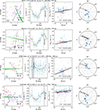 |
Fig. A.3. Diagnostic plots for RV-based spinning clusters. All the subplots are similar to Figure 4. |
| In the text | |
|
Fig. A.3. (Continued…). Diagnostic plots for RV-based spinning clusters. All the subplots are similar to those in Figure 4. |
| In the text | |
|
Fig. A.3. (Continued…). Diagnostic plots for RV-based spinning clusters. All the subplots are similar to those in Figure 4. |
| In the text | |
|
Fig. A.3. (Continued…). Diagnostic plots for RV-based spinning clusters. All the subplots are similar to those in Figure 4. |
| In the text | |
|
Fig. A.3. (Continued…). Diagnostic plots for RV-based spinning clusters. All the subplots are similar to those in Figure 4. |
| In the text | |
|
Fig. A.3. (Continued…). Diagnostic plots for RV-based spinning clusters. All the subplots are similar to those in Figure 4. |
| In the text | |
|
Fig. A.4. Diagnostic plots for PM-based spinning clusters. All the subplots are similar to those in Figure 4. |
| In the text | |
|
Fig. A.5. Diagnostic plots for expanding clusters. All the subplots are similar to those in Figure 4. |
| In the text | |
|
Fig. A.5. Continued. Diagnostic plots for expanding clusters. All the subplots are similar to those in Figure 4. |
| In the text | |
|
Fig. A.6. Diagnostic plots for contracting clusters. All the subplots are similar to those in Figure 4. |
| In the text | |
Current usage metrics show cumulative count of Article Views (full-text article views including HTML views, PDF and ePub downloads, according to the available data) and Abstracts Views on Vision4Press platform.
Data correspond to usage on the plateform after 2015. The current usage metrics is available 48-96 hours after online publication and is updated daily on week days.
Initial download of the metrics may take a while.