| Issue |
A&A
Volume 687, July 2024
Solar Orbiter First Results (Nominal Mission Phase)
|
|
|---|---|---|
| Article Number | A13 | |
| Number of page(s) | 13 | |
| Section | The Sun and the Heliosphere | |
| DOI | https://doi.org/10.1051/0004-6361/202348799 | |
| Published online | 24 June 2024 | |
Observations of fan-spine topology by Solar Orbiter/EUI: Rotational motions and indications of Alfvén waves⋆
1
Centre for mathematical Plasma Astrophysics, Mathematics Department, KU Leuven, Celestijnenlaan 200B Bus 2400, 3001 Leuven, Belgium
e-mail: This email address is being protected from spambots. You need JavaScript enabled to view it.
2
Royal Observatory of Belgium, Ringlaan -3- Av. Circulaire, 1180 Brussels, Belgium
3
Université Paris-Saclay, CNRS, Institut d’Astrophysique Spatiale, 91405 Orsay, France
4
Max-Planck-Institut für Sonnensystemforschung, Göttingen, Germany
5
Southwest Research Institute, Boulder, CO 80302, USA
Received:
30
November
2023
Accepted:
7
April
2024
Abstract
Context. Torsional Alfvén waves do not produce any intensity variation and are therefore challenging to observe with imaging instruments. Previously, Alfvén wave observations were reported throughout all the layers of the solar atmosphere using spectral imaging.
Aims. We present a torsional Alfvén wave detected in an inverted Y-shaped structure observed with the HRIEUV telescope of the EUI instrument on board Solar Orbiter in its 174 Å channel. The feature consists of two footpoints connected through short loops and a spine with a length of 30 mm originating from one of the footpoints.
Methods. We made use of the simultaneous observations from two other instruments on board Solar Orbiter. The first one is the Polarimetric and Helioseismic Imager, which is used to derive the magnetic configuration of the observed feature. The second is the Spectral Imaging of the Coronal Environment (SPICE) instrument, which provided observations of intensity maps in different lines, including Ne VIII and C III lines. We also address the issues of the SPICE point spread function and its influence on the Doppler maps via performed forward-modeling analysis.
Results. The difference movie constructed from the HRIEUV images shows clear signatures of propagating rotational motions in the spine. We measured propagation speeds of 136 km s−1–160 km s−1, which are consistent with the expected Alfvén speeds. Evidence of rotational motions in the transverse direction with velocities of 26 km s−1–60 km s−1 serves as an additional indication of torsional waves being present. Doppler maps obtained with SPICE show a strong signal in the spine region. Under the assumption that the recovered point spread function is mostly correct, synthesized raster images confirm that this signal is predominantly physical.
Conclusions. We conclude that the presented observations are compatible with an interpretation of either propagating torsional Alfvén waves in a low coronal structure or the untwisting of a flux rope. This is the first time we have seen signatures of propagating torsional motion in the corona as observed by the three instruments on board Solar Orbiter.
Key words: Sun: corona / Sun: oscillations
The difference movie is available at https://www.aanda.org.
© The Authors 2024
 Open Access article, published by EDP Sciences, under the terms of the Creative Commons Attribution License (https://creativecommons.org/licenses/by/4.0), which permits unrestricted use, distribution, and reproduction in any medium, provided the original work is properly cited.
This article is published in open access under the Subscribe to Open model. This email address is being protected from spambots. You need JavaScript enabled to view it. to support open access publication.
1. Introduction
The capabilities of solar imaging instruments have drastically advanced throughout the past couple of decades, allowing access to unprecedented spatial and temporal resolution. Therefore, modern imaging instruments provide the means for many theoretically predicted phenomena to finally be observed. The theory of magnetohydrodynamic (MHD) waves in a cylindrical geometry was developed several decades ago (Zaitsev & Stepanov 1975), and it predicted that there should be several wave modes with different characteristics in structures, for example, coronal loops and magnetic tubes filled with plasma and rooted in the solar surface (Reale 2014), that can be described by this formalism. Although observations of acoustic or kink waves are often reported (Anfinogentov et al. 2015; Gao et al. 2022; Shrivastav et al. 2024), there is still a lack of Alfvén wave observations. Ironically, Alfvén waves are one of the most potentially interesting phenomena to observe due to their ability to carry energy from the lower layers of the Sun’s atmosphere to the corona (Soler et al. 2019). In a flux tube, propagating Alfvén waves manifest themselves as rotational perturbations of the plasma velocity and azimuthal components of the magnetic field (Edwin & Roberts 1983). Since Alfvén waves are incompressible, they do not produce any intensity perturbations in the linear regime. Also, they do not exhibit displacement of the structure as, for example, kink waves, therefore making it quite challenging to observe them with imaging instruments (Van Doorsselaere et al. 2008). Hence, they are usually observed via spectral data using Doppler maps, with the signature being redshifts and blueshifts occurring simultaneously and periodic non-thermal line broadening (Erdélyi & Fedun 2007). However, when it comes to the interpretation of rotational motion observations, it is important to note that it is not only torsional Alfvén waves that manifest themselves as rotations. It has been reported by Goossens et al. (2014) that the Doppler velocity field of kink waves, depending on the line of sight, can look quite similar to what is expected from Alfvén waves.
Due to their properties, once the Alfvén waves are generated, they can easily propagate along the magnetic flux tubes (Morton et al. 2023). There are numerous reports of Alfvén wave detection in different layers of the solar atmosphere, and most of them used spectral observations, such as line broadening. Stangalini et al. (2021) reported observations of torsional oscillations in the photosphere within a magnetic pore. A study of the evolution of the magnetic field with the use of the Interferometric Bidimensional Spectropolarimeter (IBIS) revealed the presence of two out-of-phase torsional oscillations in different lobes of the pore corresponding to an azimuthal wave number of m = 1. Inferred energies exhibited an energy flux of approximately 140 kWm−2 for both lobes. Corresponding numerical simulations suggest that a kink mode could be a possible excitation mechanism of these waves.
Rotating motions are also observed in chromospheric swirls, often referred to as “magnetic tornadoes” (Shetye et al. 2019). Plasma from the chromosphere propagates upward in a spiraling motion, therefore resulting in swirl signatures. This phenomenon has garnered significant interest due to its capability to transfer mass and energy into the corona. Wedemeyer-Böhm et al. (2012) have shown that these swirls in the form of torsional Alfvén waves can provide a flux of 440 Wm−2 to the lower corona. It was numerically shown as well that indeed Alfvén waves can be generated by vortex flow in the chromosphere (Fedun et al. 2011). This energy supply is substantial enough to heat the quiet corona (Withbroe & Noyes 1977) and thus presents a potential alternative for energizing the corona. Small-scale swirls (with diameters up to 3 mm) exhibit Doppler velocities of up to 7 km s−1 and are typically associated with the motions of magnetic concentrations in the photosphere (Wedemeyer-Böhm & Rouppe van der Voort 2009).
Observations of torsional waves in the chromosphere were also reported by Jess et al. (2009). Using observations from the Swedish Solar Telescope (SST) that observed bright points in Hα, they detected variations of line width at full width half maximum (FWHM) with periods from 126 to 700 s. Combining the energy that can be carried by similar bright points over the solar surface, the waves would produce on average 240 Wm−2. De Pontieu et al. (2012) also used the data from SST to detect whether spicules of type II exhibit three types of motion: flows in a direction of the magnetic field, swaying motions, and torsional motions on the order of 25−30 km s−1. Their observed torsional motions are present in most of the spicules and represent, according to the author’s interpretation, Alfvénic waves with a speed of propagation of several hundred kilometers per second. Similar observations for spicular-type structures exhibiting high-frequency (< 50 s period) oscillations were made by Srivastava et al. (2017).
Kohutova et al. (2020) reported the first direct observations of propagating torsional Alfvén waves at coronal height using observations from AIA SDO (Lemen et al. 2012) and IRIS (De Pontieu et al. 2014). The torsional oscillation was detected in the Doppler velocity signal as the opposite edges of the flux tubes showed an antiphase oscillation. Over time the observed oscillations demonstrated an attenuation that can be explained by phase mixing. The propagation speed was estimated to be 170 km s−1. It was also shown that the observed Alfvén waves were generated as a result of a magnetic reconnection. The authors additionally suggested that small-scale reconnection events happening in twisted magnetic elements could also excite Alfvén waves (Cirtain et al. 2007).
One of the common structures occurring as a result of reconnection has a particular form, a so-called inverse Y shape (Pariat et al. 2009). It is often related to jets (Yokoyama & Shibata 1995), and its footpoints are not a mere singular bright point. Instead, they display a configuration reminiscent of a cusp or an inverted Y shape. It was introduced as a result of the observations by Shibata et al. (1994, 2007). This shape is formed as a result of reconnection between a bipole and the ambient vertical field. Reconnection produces a massive jet and generates a flux of torsional Alfvén waves.
In a similar magnetic configuration, there is a so-called fan-spine topology that is formed in a similar fashion through the emergence of a magnetic bipole into a preexisting unipolar field (Yang et al. 2020). It has been proven that this kind of topology is favorable for the occurrence of solar flares through null-point reconnection (Cheng et al. 2023). Some theoretical and numerical models have been proposed where, in this configuration, reconnection triggers a propagating torsional wave (Török et al. 2009; Pontin et al. 2011).
The current paper addresses new observations featuring a magnetic topology similar to a fan-spine configuration. We used combined observations of three instruments on board the Solar Orbiter (García Marirrodriga et al. 2021) made by the High Resolution Imager in the Extreme Ultraviolet telescope (HRIEUV) of the Extreme Ultraviolet instrument (Rochus et al. 2020), PHI (Solanki et al. 2020), and SPICE (SPICE Consortium 2020). The observed phenomenon is, therefore, tentatively interpreted as a propagating Alfvén wave. The details of the observations are given in Sect. 2. Section 3 is devoted to the analysis of the observations. In Sect. 4, we summarize and discuss the results of the findings.
2. Observations
2.1. HRIEUV data
The images were obtained on 2022 October 18 from 14:00:00 to 14:29:55 with a temporal cadence of five seconds. In our analysis, we used the data published with Data Release 5 (Mampaey et al. 2022). These observations are part of the R_SMALL_MRES_MCAD_AR_Long_Term SOOP that tracked the nearby active region for ten days1. At that time, Solar Orbiter was close to the perihelion, and its distance to the Sun constituted 0.32 au. Therefore, a pixel corresponds to 100 × 100 km2 on the Sun. There is no shared data with SDO AIA since the separation angle between the Earth and Solar Orbiter was 77.6°, and the target active region emerged on the solar limb as seen from Earth only on October 20. However, there is data from the PHI and SPICE instruments on board Solar Orbiter with the field of view (FoV) including the feature that was analyzed. Figure 1 shows an overview of the instrument’s FoVs as seen from the Solar Orbiter Full Sun Imager (FSI). The FoVs cover the targeted active region and a feature of interest for the current paper. As a preparation step for our analysis, the images taken at different times were co-aligned using the technique described by Chitta et al. (2022), with cross-correlation as a core algorithm. Figure 2 shows the first frame of the sequence of the images analyzed in the current study. The right panel of the figure shows the first frame of the running difference image.
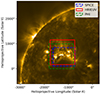 |
Fig. 1. Overview of the instrument’s FoVs as viewed from the Solar Orbiter FSI in 174 Å. Overlaid on top is the HRIEUV FoV, shown by red rectangle, and the SPICE and PHI FoVs are shown by blue and green rectangles, respectively. |
The feature that was used in our analysis was located in the northern hemisphere of the Sun. As is visible from the online movie, the structure is very dynamic. It consists of footpoints connected through short loops and a spine with a length of 30 Mm originating from one of the footpoints. There is a remote footpoint located at around [−1440″, 670″] (in helioprojective-Cartesian coordinates as seen from Solar Orbiter, denoted by the red circle in Fig. 2), where the spine is rooted back. Moreover, there is an elongated absorption feature or region with a lack of emission located to the left of the spine.
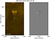 |
Fig. 2. First frame of the sequence of images taken by HRIEUV. The left panel shows the original movie. The right panel shows a running difference movie mimicking the panel on the left. The spine dynamics show untwisting motions propagating toward the remote footpoint denoted by the red circle in the left panel. A movie is available online. |
The 174 Å HRIEUV band is primarily centered around the coronal line Fe X (core temperature around 1 MK), yet it is wide enough to also encompass multiple transition region lines.
Though there are only 30 min of the dynamics depicted with HRIEUV, SPICE observations show that the spine exists for at least several hours. From both movies, original and difference, there is clear evidence of propagating material. However, apart from the propagation, there are also signatures of untwisting motion that are most clearly visible in the running difference movies. The focus of the current analysis is on the torsional motions that are observed in this spine region.
2.2. PHI data
Data acquired by the PHI High-Resolution Telescope (HRT; Gandorfer et al. 2018) was used to get an insight into the magnetic configuration of the feature. There is one magnetogram obtained at 14:15:03 with a resolution of 0.5″ per pixel, publicly available from the SOAR archive2. As a preprocessing step, the images of the HRT and EUI were co-aligned manually by visual inspection such that the fan region located to the north side of the spine and active region loops (shown by red dashed curves in Fig. 3, panel a) on the west of the feature would match regions with magnetic field enhancements. The active region loops originate from the sunspot shown by black circle.
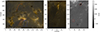 |
Fig. 3. Magnetograms obtained with PHI HRT. Panel a shows the cropped FoV of HRIEUV imposed on top of the HRT view. The blue rectangle shows the location of the spine. Red dashed curves show identified loops used for alignment purposes. The black dashed circle shows a sunspot near the spine. Panel b shows a zoomed-in view of the feature. Panel c shows a PHI zoomed-in view alone. Red dashed circles show the footpoint at the origin of the spine and the footpoint corresponding to the remote brightening. |
Figure 3a shows the cropped FoV of both telescopes aligned with each other. From the comparison, we judged the alignment to be sufficiently accurate for the purposes of this work. Panels b and c in Fig. 3 show that there are bipolar magnetic field concentrations corresponding to the short loop footpoints at the base of the spine. Apart from that, there is a strong negative magnetic field corresponding to the location where the spine is rooted. And for the remote footpoint of the spine, there is a magnetic field of opposite polarity. Therefore, the magnetic configuration, in this case, resembles the fan-spine configuration described in Yang et al. (2020), as shown in Fig. 4a.
 |
Fig. 4. Magnetic configuration of the spine and the propagating pulse. Panel a shows the sketch of magnetic structure. Courtesy of Yang et al. (2020). The purple spiral shows the propagation of an Alfvén wave. Panel b illustrates the propagation of one single Alfvén wave pulse. |
A potential field extrapolation shown in Fig. 5 confirmed the presence of a coronal null point and, by that, of the fan-spine topology. The spine in the extrapolation is, however, not oriented in the north-south direction (as in the observation), likely due to a lack of information of the magnetic field on a large scale, outside of the PHI FoV. However, we used the extrapolation to gain approximate information about the scaling of the magnetic field along the spine, which must be taken as an order of magnitude estimate only. The spine starts from 177 G in the photosphere to zero in the null. As it keeps rising in height, it reaches 13 G at the spine top. The spine then bends down, and correspondingly, the magnetic field strength increases up to 220 G at the photospheric footpoint. The purple spiral in Fig. 4a shows the propagation of a torsional Alfvén wave. The Alfvén wave in this case looks like a propagating twist that is shown in Fig. 4b.
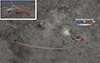 |
Fig. 5. Field line rendering of the potential field in the vicinity of the null point. The background image represents the radial magnetic field saturated between −800 and 800 G; field lines are colored with the potential field magnitude, in logarithmic scale. The top-left inset shows an enlarged side-view of the null region. |
2.3. SPICE data
SPICE ran a dynamic sequence, rastering with the 4″ slit and a step of 6″ to give a field of view of 766″ × 768″, with a five-second exposure time. While the pixel size is 4″ × 1″, the spatial resolution is dominated by a point spread function (PSF), which we discuss in the Sect. 3.1. For the present analysis, we used four spectral windows that include the following lines profiles: H I Lyβ 1025.72 Å (log Te = 4.0 K); C III 977.03 Å (log Te = 4.8 K); Ne VIII 770.42 Å (log Te = 5.8 K); and Mg IX 706.02 Å (log Te = 6.0 K). This selection is the most representative of different layers of the solar atmosphere.
We used L2 data (data release 33) that were corrected for instrumental artifacts and radiometrically calibrated to create the intensity and Doppler maps through a Gaussian fitting of the spectral lines. As the cadence of the SPICE raster is 12 min, there are three raster images obtained for the whole period of the feature observed by HRIEUV. They are shown in Fig. 6, where each row corresponds to a different spectral line. Figure 6 shows the multi-thermal nature of the structure, and at each time period (i.e., a given raster position), brightenings dominate in different areas for the three temperatures.
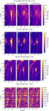 |
Fig. 6. Intensity maps obtained with SPICE for four different lines starting from the cool chromosphere and incrementally increasing up to the coronal temperatures. The first row shows three consecutive frames (14:02:59, 14:14:28, and 14:25:57) for the H I Lyβ line, the second row shows intensity maps for the C III line, and the two last rows show intensity maps for the Ne VIII and Mg IX lines, correspondingly. |
The depicted temperature of the Ne VIII spectral line is the closest to the HRIEUV 174 Å channel’s peak temperature and is shown in the g–i panels of Fig. 6. Therefore, there we observed intensity enhancements with approximately the same shapes: the spine and two bundles of loops on the left side. Over the 30 min of recording, the intensity shows local enhancement and dimming, confirming the short timescale dynamic seen in HRIEUV, while remaining about constant as a whole. In cooler lines, such as H I Lyβ (panels a–c) and C III (panels d–f) in the first frame, there is an intensity enhancement following the whole feature. As for the consecutive frames, the intensity enhancement is much weaker in the spine region, and the fan region appears dimmer.
The C III line shows the highest intensity enhancement, hinting at the fact that the spine has a counterpart at the chromospheric temperature. However, when it comes to the hotter line, Mg IX (shown by panels j–l in Fig. 6), the feature is not visible at all, pointing out the fact that the plasma temperatures at this region correspond to chromospheric and low-transition region temperatures.
3. Data analysis
In order to estimate the propagation speed of the material, we constructed time-distance maps based on HRIEUV images. The region for the time-distance map is indicated in Fig. 7a with red dashed lines, and that region was chosen such that it encompasses the spine in the transverse direction. The expected Alfvén speed  is around 180 km s−1, assuming the plasma density of the spine material is 10−10 kg m−3, as in Kohutova et al. (2020), and taking the magnetic field strength of 20 G as derived from extrapolation. The density assumption is based on data from SPICE that confirms that the plasma comprising the spine exhibits transition region and chromospheric temperatures. Since the uncertainty in the Alfvén speed depends solely on this density assumption, its error is half that of the density error. In the current case, the measured propagation velocities are indicated in Fig. 7b and are consistent with the expected Alfvén speed of 130 km s−1 to 180 km s−1 for the beginning of the sequence (Kohutova et al. 2020).
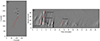 |
Fig. 7. Time-distance map demonstrating the propagation. Panel a shows a snapshot of the difference movie with the highlighted region (red dashed curves) that was used to create a time-distance map. Panel b shows the time-distance map where propagating material is clearly visible. Red lines represent fits to the propagating wave fronts with their annotated values of propagation velocity. |
Apart from the fact that the movie shown by Fig. 2 shows untwisting propagating motion, we can use the same technique used by Long et al. (2023) as another qualitative evidence of the presence of rotational motions. The idea is to construct a series of running ratios where values of intensities corresponding to one time frame are divided by the intensities corresponding to previous time frame. This way, the propagation of the pixels with a higher intensity can be tracked. The obtained running ratios are shown in Fig. 8. The limit of the pixels that were plotted was identified empirically via testing different cutoff values and, the limits are different for each time range shown, varying from 1.18 to 1.3. Points of blue and purple in the figure correspond to the beginning of the sequence, and the yellow and red colors correspond to the end of the sequence. While there might be blue and red colors present on the opposite edges of the spine, it does not necessarily mean that this is evidence of a torsional motion. However, if there is a region where the color of the pixels changes smoothly from blue to red throughout the whole color sequence of the color bar, it would indicate that we are following the same plasma blob through different time frames. Therefore, if this motion is directed not along the spine but across it, this can be considered as a signature of side-to-side or rotational motion. While this is only a qualitative indication of the rotation motions, one of the quantitative ways is to construct transverse slits and analyze the produced time-distance maps for movement across the axis of the spine.
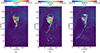 |
Fig. 8. Snapshots of running ratios plotted on top of the HRIEUV images. The white arrows represent the direction of plasma material movement. The color bar represents intervals of time used to construct the running ratio. |
To illustrate the localization of the wave pulse, images were generated using the same technique, plotting color-coded points obtained through the calculation of running ratios (Fig. 9). Here, the presentation is frame by frame, with each frame separated by five seconds, facilitating the tracing of the pulse’s propagation. Panels b–h depict a zoomed-in view of the red rectangle in panel a. The red dashed ellipse highlights the pulse being tracked. It can be observed that as time progresses through panels b and c, the pulse moves toward the west and south. As depicted in the figure, the pulse is localized, as shown by the sequence of figures, approximately 10 × 20 HRIEUV pixels, which is much smaller than the spine itself.
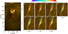 |
Fig. 9. Snapshots of running ratios. Panel a shows the spine, where the red rectangle highlights the area of interest. Panels b–h display zoomed-in views corresponding to different time frames starting from 14:01:40 and separated by five seconds. Points are colored according to the time, with the color bar shown at the top. |
Figure 10 shows the time-distance maps constructed from the slits that are indicated on Fig. 10a by white dashed lines. In order to measure the propagation speed of the plasma, in each frame the intensity was fitted with a Gaussian function across, and the obtained centroids were fitted with a line (as denoted in Fig. 10c, e, and g). The determined angle of the line was translated into physical speeds that constitute 26 km s−1 for slit 1, 37.7 km s−1 for slit 2, and 56.3 km s−1 for slit 3.
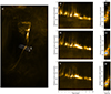 |
Fig. 10. Time-distance maps demonstrating the transverse motion. Slits used to construct time-distance maps are shown by white dashed lines (left column). Numbers denote the number of each slit. Time-distance maps were constructed from the slits taken across the spine (middle column) to show the evidence of the movement in the transverse direction. The third column shows a zoomed-in view with the points fitted to the propagating pulse. The zoomed-in view is indicated by a blue rectangle in each figure in the middle column. |
The obtained values of the rotational velocities hint toward the Doppler velocities that can be expected from the spectral measurements from SPICE. Moreover, we note the amplitudes of the observed waves. On average, they constitute 20%−30% of the local Alfvén speed, indicating that the linear regime assumptions cannot be applied in this case, and thus a non-linear regime is entered.
3.1. Doppler maps
In this section, we analyse the Doppler maps in order to find line-of-sight evidence of torsional waves. According to Plowman et al. (2023), the PSF of SPICE is elongated in spectral (λ) and slit-aligned (y) directions and tilted by approximately 15° in the (y − λ) plane. The tilt in the spatial-spectral plane results in the creation of an illusionary dim feature next to a bright feature, and this results in the creation of artificial signals in the Doppler maps following intensity gradients.
Figure 11 shows the C III intensity and Doppler maps obtained by SPICE for the three different times. Pixels that have a very low signal in the intensity maps and zero velocity in the Doppler maps appear as white. The location of the spine is denoted by the white rectangle in Fig. 11a. There are two distinct locations to note in the Doppler maps: the region that corresponds to the high intensity gradient (shown by the black ellipse) and the region that does not (shown by the magenta ellipse in panel b). Across all time frames, the Doppler maps consistently display a pronounced, strong blueshift in the region marked by the black ellipse. However, the area identified by the magenta ellipse only exhibits a discernible signal, distinguishable from noise, in panel b. Moving to the next time frame, as depicted in panel d, strong redshifts appear to the left of the spine, possibly associated with an absorption feature, and it is hard to say if the signal is physical or artificial. Panel f shows some level of redshift, but it is hard to make any conclusions about its nature. While it is known that the earlier described PSF issues of SPICE can create an artificial signal in Doppler maps, torsional waves as well produce Doppler shifts, as it is one of the primary detection features for this phenomenon. Therefore, most likely, the maps obtained by SPICE have a combination of real and artificial signals, and it is important to be able to separate one from the other. In order to estimate the influence of the tilted SPICE PSF, synthetic raster spectra were made using HRIEUV 174 Å data as an input.
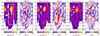 |
Fig. 11. Intensity and Doppler maps obtained with the SPICE C III line for three time frames (14:02:59, 14:14:28, and 14:25:57). Panels a and b show maps for the first time frame, panels c and d are for the second, and panels e and f are for the last frame. The white rectangle in panel a shows the location of the spine. Black ellipses in panels b, d, and f show the location of a strong signal that matches the high intensity gradient in panel a. The magenta ellipse in panel b shows the location of a strong Doppler signal that does not correspond to the high intensity gradient. |
It is important to mention that the synthesized images correspond only partially to the temperatures the SPICE lines depict. Therefore, it is impossible to fully reproduce SPICE images, which potentially can lead to the different behavior shown in both the intensity and Doppler maps. Although the Ne VIII line has the closest temperature coverage to the 174 Å channel, its intensity is much smaller compared to the CIII line. For this reason, it makes more sense to compare the modeled intensity maps with that of the SPICE Ne VIII line. However, when it comes to Doppler maps, the Ne VIII line does not show any signal due to the mentioned weak signal issue. Therefore, we compared the Doppler maps to those from the CIII line.
The EUI images needed to be scanned as was done by SPICE. The exposure time for SPICE is five seconds, and the slit width is 4″ with a step of 6″, which for HRI with a pixel resolution of 0.5″ means that every five seconds a column with the width of eight pixels in HRI is saved. However, the non-zero width of the slit means that after every eight columns of HRI data being saved, there are four columns of data being lost. As a result, we had a scanned image with the resolution of HRI. Therefore, the next step was to downsample the scanned image to the SPICE resolution.
The next step was to supplement the data with a spectral dimension. The width of an observed emission line is defined by the thermal broadening, non-thermal motions, and instrumental broadening and can be expressed as follows in terms of the FWHM:
The thermal broadening was calculated from the peak temperature T = 0.8 MK of the 174 Å channel as follows:
 (1)
(1)
where kB is the Boltzmann constant, c is the speed of light, λ0 is the expected centroid wavelength of the line (which is 174 Å in our case), and mion is the mass of the emitting ion. The condition of λ = λ0 results in zero Doppler shift.
The non-thermal broadening wnth can be caused by several different processes, including turbulence (Pontin et al. 2020), small-scale flows (De Pontieu et al. 2015), and waves (Chae et al. 1998). According to Chae et al. (1998), the coronal non-thermal velocity is equal to 20 km s−1, and therefore, this value was used for our analysis.
However, the line width in SPICE is dominated by the instrumental width wI. As described in Fludra et al. (2021), the FWHM (estimated for 2″ slit) for the short wavelength (SW) band is estimated to be eight pixels and nine pixels for the long wavelength (LW) band. This corresponds to Doppler velocities of 200 km s−1. The PSF is not completely known for the 4″ slit, so we used the properties derived for the 2″ slit. Next, knowing the parameters of the Gaussian and the peak intensity Ip in each pixel, we could construct a wavelength dimension as it would have been observed by SPICE:
![Mathematical equation: $$ \begin{aligned} I = I_{\rm p}\cdot \mathrm{exp}\left[- \frac{(\lambda -\lambda _0)^2}{2\sigma ^2}\right], \end{aligned} $$](/articles/aa/full_html/2024/07/aa48799-23/aa48799-23-eq4.gif) (2)
(2)
where the width of the Gaussian σ is related to the FWHM w through  . As a result, we obtained a 3D cube of the data that we then convolved with the SPICE PSF in (y − λ) space as described in Plowman et al. (2023).
The last step for this simulation was to fit the intensities in the wavelength dimension with a Gaussian again to obtain the Doppler shifts. The total intensity was obtained by integration of the Gaussian over a wavelength range. Poisson noise that depends on intensity such that it is comparable to noise in SPICE was added. The results (for the time frame 14:14:28) are shown in Fig. 12. Panel a shows intensities obtained from line fitting, and panel b shows the Doppler map.
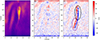 |
Fig. 12. Synthesized spectral rasters obtained using forward-modeled analysis. Panel a shows the synthesized intensity, while the panels b and c show the Doppler maps (mimicking the SPICE CIII line) with and without local velocities imposed on top of the feature. The black ellipse in panel c shows the location of a strong signal that corresponds to the high intensity gradient. The magenta ellipse outlines the location that does not correspond to any intensity gradient. |
This simulation alone, however, is not enough to distinguish between a signal caused by rotational motions and artificial PSF signal contributions in SPICE Doppler maps. For that, we performed another simulation in a similar fashion but with the local Doppler velocities imposed on top of the feature. The model for the velocity field was chosen to be a simple case of a rigid body rotation. Details of the velocity field are given in Appendix A. The result is shown in Fig. 12c.
With that being said, the synthesized intensity map depicted by Fig. 12a follows the same shape as observed by the SPICE C III and Ne VIII lines shown in second and third rows of Fig. 6. Specifically, the latter reproduces the signal coming from the loops located to the left of the spine. Similarly, the signal coming from the spine weakens for lower values of the y-coordinate.
The base of the feature is more extended (about six columns in the C III raster) than the dome (Ne VIII, four columns). The synthetic raster created using HRIEUV resembles but is not precisely identical to the Ne VIII. The shape is something between Ne VIII and C III. This suggests that the dynamics within the feature are associated with multi-thermal plasma evolution not completely caught by the HRIEUV. We suggest that the torsional waves are within these multi-thermal structures.
As expected from the effects of the PSF, panel b with the Doppler maps without local velocities imposed shows that there is a signal following the gradients of the intensity region matching the signal from the loops and the spine. The signal in the spine region reaches a maximum of 20 km s−1 for both blueshifts and redshifts. The map with the velocities imposed depicted by panel c understandably shows a strong signal following the central lines of the rotation reaching up to 60 km s−1, which is comparable to values measured by SPICE. To match the synthetic spectra with observations, Fig. 12c should be compared to the Fig. 11b. The signal is modulated by the effect of the PSF, leading to various non-uniformities, as opposed to the imposed velocity field coming from the intensity gradients. While the redshifts are present in panel b of Fig. 11, the strong blueshifts are the new phenomenon that matches the SPICE observations, indicating that this signal should be physical under the assumption that the recovered PSF is correct.
Furthermore, a notably strong Doppler signal persists in a region marked by the magenta ellipse in Fig. 12c, even in the absence of a locally imposed velocity. Considering that there are no intensity enhancements in the lower spine region, the fact that both the synthesized and observed images exhibit a signal provides substantial evidence for its authenticity under the assumption that the recovered PSF is mostly correct.
3.2. Magnetic field perturbation
With the use of the Elsässer variables, one can estimate the perturbated magnetic field compared to the background field. In incompressible MHD counterpropagating waves are described by Elsässer variables  , where V is the velocity of the plasma, B is the magnetic field, and μ and ρ are the magnetic permeability and density (Elsasser 1950). Positive corresponds to an outward propagating wave and negative to an inward propagating wave. For our case, we have z−, which equals zero since we have an Alfvén wave. With the use of the perturbed over equilibrium variables (denoted with index zero and with no assumption on its amplitude) and background variables, the expression can be written as follows:
Working with the absolute values of vectors, one can deduce the perturbed magnetic field:
Taking estimates from the observations for the velocities and magnetic field of 20 G from the extrapolation, we concluded that the perturbed magnetic field should be around 4.5 G.
4. Discussion and conclusion
Through the current study, we have presented observations of a dynamic fan-spine topology consisting of a spine feature. This feature was observed by the EUI HRIEUV, PHI HRT, and SPICE instruments on board Solar Orbiter. The movies constructed from the HRIEUV observations give a strong impression of torsional motions in the spine structure. In this work, we have confirmed these torsional motions from the base of the spine southward (Fig. 8) and into the spine by showing the simultaneous presence of southward longitudinal motions (Fig. 7), transverse motions in the plane of sky (Fig. 10), and line-of-sight motion (Fig. 11). In addition, since these torsional motions have a speed consistent with a local estimate of the Alfvén speed, we tentatively identified these torsional motions as torsional Alfvén waves.
There is a signature of torsional motions visible in the difference and original movies. Possible evidence of this signature can also be found in the time-distance maps obtained from transverse cuts with velocities in the transverse direction constituting 26−56 km s−1. Running ratios also point out the fact that there is indeed not only the propagation of the matter but also side-to-side motion. The measured propagation speed constitutes values of 130−180 km s−1, which is consistent with the expected values of Alfvén speed and similar to what has been measured by Kohutova et al. (2020). Moreover, the performed forward modeling serves as an additional argument to the possible interpretation of the observed phenomenon to be torsional motion, as it shows that there is a Doppler signal in a region corresponding to the spine. While this analysis is beneficial for the current work, it may also be used to gain an insight into the reliability of SPICE Doppler maps, and the instrument’s ability to detect rotational or line-of-sight movements.
However, the issue of artifacts appearing in the Doppler maps is quite complicated, and it has recently been recognized that the PSF is not the sole source of the false signal. Additional sources, such as the “overlappograph” (Tousey et al. 1977) can create a Doppler shift when a bright feature is present on one side of the slit. This effect is weaker when the emission is less sharp, which appears to be the case for the HRIEUV 174 Å channel when compared to the SPICE lines. Nevertheless, reproducing this effect in current simulations poses a challenge. Consequently, efforts to untangle the artificial signal from the physical one are still ongoing, and further work is necessary to achieve this goal.
One of the primary signatures of these oscillations is their substantial amplitude. The velocity in the transverse direction accounts for 30% of the local Alfvén speed, indicating that these waves exist within a non-linear regime. This observation would be a prime example to look for non-linear effects of Alfvén waves, due to their extremely high velocity amplitude. One could look for steepening wave fronts, turbulence formation, or the existence of solitons or solitary waves.
As a result of the significant velocity amplitude of these waves, the energy budget becomes considerably high. Computed using the formula E = ρv2VA, it reaches magnitudes on the order of tens of kilowatts per square meter, although it is important to acknowledge that this estimate is susceptible to errors arising from density assumption and velocity calculations. However, it is notably greater than the calculated energy that should be transferred to the corona, as estimated by Jess et al. (2009), De Pontieu et al. (2007). This estimated energy transfer should be on par with the findings in Kohutova et al. (2020). While Kohutova et al. (2020) does not provide a direct calculation of the energy, the input parameters used therein are comparable to those in the current manuscript, thereby yielding similar flux values. As for the driver of those oscillations, it is still a point of question. It has been previously observed, for example, by Kohutova et al. (2020) that torsional waves can be triggered by reconnection, which is happening in this case. Moreover, Pariat et al. (2009) has shown that null point reconnection can release the twist in a jet. However, the fact that hotter SPICE lines such as Mg IX do not have any signal at all shows that the temperature does not increase up to a point of log T = 6.0 K, thus serving as an argument against reconnection as a potential wave exciter candidate.
It is important to mention, however, that there are alternative interpretations of the event such as a propagating kink wave with circular polarization (Magyar et al. 2022). With the available data and no shared view from another vantage point, there is no possibility to differentiate between those two interpretations. Additionally, torsional motions of the coronal structure may be considered as evidence of torsional Alfvén waves, but other interpretations, such as the untwisting of a flux rope (Li et al. 2015; Liu et al. 2009), cannot be ruled out. There are following factors to take into account when distinguishing between the two interpretations:
-
Accurate estimation of the Alfvén speed in the observed spine is impossible without differential emission measure (DEM) analysis of the structure. However, as mentioned in Sect. 2, there is no shared data with the SDO AIA, and the SPICE instrument on board Solar Orbiter lacks sufficient spectral lines to conduct a DEM analysis. Given these circumstances, we assume the density value. However, since the Alfvén speed is only influenced by the square root of the density, even with an order of magnitude difference from the actual density, the Alfvén speed would only vary by a factor of three.
-
Due to the projection effect, the torsional motion of the spine can become apparent. For example, it can be attributed to the antiparallel motion of different plasma layers along the line of sight.
-
The SPICE time cadence is too high to capture the prominent wave dynamics. However, high cadence spectral data is not necessarily required to confirm the presence of waves, as no periodicity is expected if the driver launches pulses. The current cadence of 12 min is sufficient to support the conclusion that there is line-of-sight evidence of torsional motions.
-
The consideration of pulse size is also necessary. Figures 11 and 12 may suggest that the pulse size is equal to the spine’s size, supporting the interpretation of the untwisting of a flux rope. However, the width of the pulse in the mentioned figures is not spatially resolved, and it is determined by the SPICE slit width and the scanning speed. As for Fig. 12, this is the case because the velocity field is imposed based on the model of rigid body rotation. Therefore, for simplicity, we assume that the body rotates as a whole.
-
The observations of the torsional motions in 174 Å intensity maps and in C III Doppler maps are not necessarily attributed to one phenomenon because the line temperatures differ significantly. Though it is true, the intensity signal in NeVIII is much smaller compared to the CIII line. Consequently, the Ne VIII line does not exhibit any signal in the Doppler maps that would overpower the noise level.
Considering the points described above, we lean more toward the interpretation of propagating torsional Alfvén waves. However, it is also worth noting that the possibility of an untwisting motion cannot be entirely ruled out.
Movie
Movie 1 associated with Fig. 2 (aa48799movie) Access Supplementary Material
See https://www.mps.mpg.de/solar-physics/solar-orbiter-phi/data-releases for more information about the employed PHI data release.
Acknowledgments
Solar Orbiter is a space mission of international collaboration between ESA and NASA, operated by ESA. The EUI instrument was built by CSL, IAS, MPS, MSSL/UCL, PMOD/WRC, ROB, LCF/IO with funding from the Belgian Federal Science Policy Office (BELSPO/PRODEX PEA 4000112292); the Centre National d’Etudes Spatiales (CNES); the UK Space Agency (UKSA); the Bundesministerium für Wirtschaft und Energie (BMWi) through the Deutsches Zentrum für Luft- und Raumfahrt (DLR); and the Swiss Space Office (SSO). We are grateful to the ESA SOC and MOC teams for their support. The German contribution to SO/PHI is funded by the BMWi through DLR and by MPG central funds. The Spanish contribution is funded by AEI/MCIN/10.13039/501100011033/ and European Union “NextGenerationEU/PRTR” (RTI2018-096886-C5, PID2021-125325OB-C5, PCI2022-135009-2, PCI2022-135029-2) and ERDF “A way of making Europe”; “Center of Excellence Severo Ochoa” awards to IAA-CSIC (SEV-2017-0709, CEX2021-001131-S); and a Ramón y Cajal fellowship awarded to DOS. The French contribution is funded by CNES. The development of SPICE has been funded by ESA member states and ESA. It was built and is operated by a multi-national consortium of research institutes supported by their respective funding agencies: STFCRAL (UKSA, hardwarelead), IAS (CNES, operationslead), GSFC (NASA), MPS (DLR), PMOD/WRC (SwissSpaceOffice), SwRI (NASA), UiO (NorwegianSpaceAgency). T.V.D. was supported by the C1 grant TRACEspace of Internal Funds KU Leuven. E.P. has benefited from the funding of the FWO Vlaanderen through a Senior Research Project (G088021N).
References
- Anfinogentov, S. A., Nakariakov, V. M., & Nisticò, G. 2015, A&A, 583, A136 [NASA ADS] [CrossRef] [EDP Sciences] [Google Scholar]
- Chae, J., Schühle, U., & Lemaire, P. 1998, ApJ, 505, 957 [NASA ADS] [CrossRef] [Google Scholar]
- Cheng, X., Priest, E. R., Li, H. T., et al. 2023, Nat. Commun., 14, 2107 [Google Scholar]
- Chitta, L. P., Peter, H., Parenti, S., et al. 2022, A&A, 667, A166 [NASA ADS] [CrossRef] [EDP Sciences] [Google Scholar]
- Cirtain, J. W., Golub, L., Lundquist, L., et al. 2007, Science, 318, 1580 [Google Scholar]
- De Pontieu, B., McIntosh, S., Carlsson, M., et al. 2007, Science, 318, 1574 [NASA ADS] [CrossRef] [Google Scholar]
- De Pontieu, B., Carlsson, M., Rouppe van der Voort, L. H. M., et al. 2012, ApJ, 752, L12 [Google Scholar]
- De Pontieu, B., Title, A. M., Lemen, J. R., et al. 2014, Sol. Phys., 289, 2733 [Google Scholar]
- De Pontieu, B., McIntosh, S., Martinez-Sykora, J., Peter, H., & Pereira, T. M. D. 2015, ApJ, 799, L12 [Google Scholar]
- Edwin, P. M., & Roberts, B. 1983, Sol. Phys., 88, 179 [Google Scholar]
- Elsasser, W. M. 1950, Phys. Rev., 79, 183 [Google Scholar]
- Erdélyi, R., & Fedun, V. 2007, Science, 318, 1572 [CrossRef] [Google Scholar]
- Fedun, V., Verth, G., Jess, D. B., & Erdélyi, R. 2011, ApJ, 740, L46 [Google Scholar]
- Fludra, A., Caldwell, M., Giunta, A., et al. 2021, A&A, 656, A38 [NASA ADS] [CrossRef] [EDP Sciences] [Google Scholar]
- Gandorfer, A., Grauf, B., Staub, J., et al. 2018, in Space Telescopes and Instrumentation 2018: Optical, Infrared, and Millimeter Wave, eds. M. Lystrup, H. A. MacEwen, G. G. Fazio, et al., SPIE Conf. Ser., 10698, 106984N [Google Scholar]
- Gao, Y., Tian, H., Van Doorsselaere, T., & Chen, Y. 2022, ApJ, 930, 55 [NASA ADS] [CrossRef] [Google Scholar]
- García Marirrodriga, C., Pacros, A., Strandmoe, S., et al. 2021, A&A, 646, A121 [CrossRef] [EDP Sciences] [Google Scholar]
- Goossens, M., Soler, R., Terradas, J., Van Doorsselaere, T., & Verth, G. 2014, ApJ, 788, 9 [CrossRef] [Google Scholar]
- Janvier, M., Mzerguat, S., Young, P. R., et al. 2023, A&A, 677, A130 [NASA ADS] [CrossRef] [EDP Sciences] [Google Scholar]
- Jess, D. B., Mathioudakis, M., Erdélyi, R., et al. 2009, Science, 323, 1582 [Google Scholar]
- Kohutova, P., Verwichte, E., & Froment, C. 2020, A&A, 633, L6 [NASA ADS] [CrossRef] [EDP Sciences] [Google Scholar]
- Lemen, J. R., Title, A. M., Akin, D. J., et al. 2012, Sol. Phys., 275, 17 [Google Scholar]
- Li, X., Yang, S., Chen, H., Li, T., & Zhang, J. 2015, ApJ, 814, L13 [NASA ADS] [CrossRef] [Google Scholar]
- Liu, W., Berger, T. E., Title, A. M., & Tarbell, T. D. 2009, ApJ, 707, L37 [NASA ADS] [CrossRef] [Google Scholar]
- Long, D. M., Green, L. M., Pecora, F., et al. 2023, ApJ, 955, 152 [CrossRef] [Google Scholar]
- Magyar, N., Duckenfield, T., Van Doorsselaere, T., & Nakariakov, V. M. 2022, A&A, 659, A73 [NASA ADS] [CrossRef] [EDP Sciences] [Google Scholar]
- Mampaey, B., Verbeeck, F., Stegen, K., et al. 2022, SolO/EUI Data Release 5.0 2022-04 (Royal Observatory of Belgium) [Google Scholar]
- Morton, R. J., Sharma, R., Tajfirouze, E., & Miriyala, H. 2023, Rev. Mod. Plasma Phys., 7, 17 [NASA ADS] [CrossRef] [Google Scholar]
- Pariat, E., Antiochos, S. K., & DeVore, C. R. 2009, ApJ, 691, 61 [Google Scholar]
- Plowman, J. E., Hassler, D. M., Auchère, F., et al. 2023, A&A, 678, A52 [NASA ADS] [CrossRef] [EDP Sciences] [Google Scholar]
- Pontin, D. I., Al-Hachami, A. K., & Galsgaard, K. 2011, A&A, 533, A78 [NASA ADS] [CrossRef] [EDP Sciences] [Google Scholar]
- Pontin, D. I., Peter, H., & Chitta, L. P. 2020, A&A, 639, A21 [NASA ADS] [CrossRef] [EDP Sciences] [Google Scholar]
- Reale, F. 2014, Liv. Rev. Sol. Phys., 11, 4 [Google Scholar]
- Rochus, P., Auchère, F., Berghmans, D., et al. 2020, A&A, 642, A8 [NASA ADS] [CrossRef] [EDP Sciences] [Google Scholar]
- Shetye, J., Verwichte, E., Stangalini, M., et al. 2019, ApJ, 881, 83 [Google Scholar]
- Shibata, K., Nitta, N., Strong, K. T., et al. 1994, ApJ, 431, L51 [Google Scholar]
- Shibata, K., Nakamura, T., Matsumoto, T., et al. 2007, Science, 318, 1591 [Google Scholar]
- Shrivastav, A. K., Pant, V., Berghmans, D., et al. 2024, A&A, 685, A36 [NASA ADS] [CrossRef] [EDP Sciences] [Google Scholar]
- Solanki, S. K., del Toro Iniesta, J. C., Woch, J., et al. 2020, A&A, 642, A11 [NASA ADS] [CrossRef] [EDP Sciences] [Google Scholar]
- Soler, R., Terradas, J., Oliver, R., & Ballester, J. L. 2019, ApJ, 871, 3 [Google Scholar]
- SPICE Consortium (Anderson, M., et al.) 2020, A&A, 642, A14 [NASA ADS] [CrossRef] [EDP Sciences] [Google Scholar]
- Srivastava, A. K., Shetye, J., Murawski, K., et al. 2017, Sci. Rep., 7, 43147 [Google Scholar]
- Stangalini, M., Erdélyi, R., Boocock, C., et al. 2021, Nat. Astron., 5, 691 [NASA ADS] [CrossRef] [Google Scholar]
- Török, T., Aulanier, G., Schmieder, B., Reeves, K. K., & Golub, L. 2009, ApJ, 704, 485 [Google Scholar]
- Tousey, R., Bartoe, J. D. F., Brueckner, G. E., & Purcell, J. D. 1977, Appl. Opt., 16, 870 [NASA ADS] [CrossRef] [Google Scholar]
- Van Doorsselaere, T., Nakariakov, V. M., & Verwichte, E. 2008, ApJ, 676, L73 [Google Scholar]
- Wedemeyer-Böhm, S., & Rouppe van der Voort, L. 2009, A&A, 507, L9 [NASA ADS] [CrossRef] [EDP Sciences] [Google Scholar]
- Wedemeyer-Böhm, S., Scullion, E., Steiner, O., et al. 2012, Nature, 486, 505 [Google Scholar]
- Withbroe, G. L., & Noyes, R. W. 1977, ARA&A, 15, 363 [Google Scholar]
- Yang, S., Zhang, Q., Xu, Z., et al. 2020, ApJ, 898, 101 [Google Scholar]
- Yokoyama, T., & Shibata, K. 1995, Nature, 375, 42 [Google Scholar]
- Zaitsev, V. V., & Stepanov, A. V. 1975, Issled. Geomagn. Aeron. Fiz. Solntsa, 37, 3 [NASA ADS] [Google Scholar]
Appendix A: Local velocity field and spectra
As mentioned above, local Doppler velocities were imposed on top of the feature for the forward-modeling analysis. The model for the velocity field is a rigid body rotation. Therefore, since the current feature has a complex shape, it was fitted with two lines as shown in Fig. A.1 (a) by black dashed lines. They were used as two central lines with the imposed velocity field as shown in Fig. A.1 (b). Values of the velocity were taken such that they would correspond to the observed values of velocities in the transverse direction as obtained in Section 3. The line in the x direction, where negative velocities transit to positive velocities, corresponds to the central line around which rotation is happening.
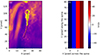 |
Fig. A.1. The model of the rigid body rotation. Central lines of the feature identified in rigid body rotation are denoted by dashed black lines (panel (a)). Panel (b) depicts the velocity field imposed on top of the feature. |
Then, the described velocity field was used to construct a wavelength dimension similar to Eq. 2:
![Mathematical equation: $$ \begin{aligned} I = I_p\cdot \mathrm{exp}\left[- \frac{1}{2\sigma ^2}\left(\left(\lambda -\lambda _0\left(1-\frac{v}{c}\right)\right)\right)\right]. \end{aligned} $$](/articles/aa/full_html/2024/07/aa48799-23/aa48799-23-eq9.gif) (A.1)
(A.1)
Figure B.1 displays the spectra for a specific slit position in SPICE, as illustrated in panel (a), and for the modeled data, depicted in panel (b). The slit was chosen to pass through the spine region. The intensity maps were aligned to ensure that the slit position traverses the same intensity feature. However, differences in spectra still persist because the channels depict different plasma temperatures. This discrepancy is the reason for the varying number of blobs observed along the slit. Nevertheless, the presence of rotation and elongation in the PSF is evident, particularly in B.1 (b).
Appendix B: Proxy for the instrumentally generated velocity
An alternative way to check if the signal in the SPICE Doppler maps is generated by the PSF tilt is to estimate the intensity gradients as it was done by Janvier et al. (2023). False velocity signals exhibit correlations with image intensity gradients, particularly those aligned with the slit direction, with a smaller contribution from intensity gradients perpendicular to the slit. We followed the procedure described by Janvier et al. (2023) in Appendix B and constructed the intensity gradients for the intensity map obtained by SPICE and shown in Fig. 6 (a). Next, the intensity gradient in each pixel was plotted against the estimated Doppler velocity in that pixel, and a linear fit was performed. However, it is important to note that the linear fit is not necessarily the best choice due to the high level of spreading of the points. Figure 1 (a) shows a negative correlation between the Doppler velocity obtained with SPICE and the intensity gradient along the slit similar to Janvier et al. (2023). Contrary to the results of Janvier et al. (2023), Fig. 1 (b) shows a relatively strong positive correlation between velocities and intensity gradients across the slit. The ±1σ region was not included in order to perform the linear fit, as it is assumed to have a physical origin.
Finally, the slopes of the line fits were multiplied by the intensity gradients, and the resulting maps were summed together to create the overall proxy map shown in panel (a) of Fig. B.3 (which also has units of velocities). Here, the white regions correspond to the areas with a minimal risk of getting a false signal.
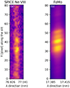 |
Fig. B.1. Spectra from a particular slit position in SPICE and forward-modeled data. The slit is passing through the spine region. |
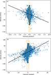 |
Fig. B.2. Relation between the intensity gradients along (panel (a)) and across (panel (b)) the SPICE slit with the Doppler velocities. The orange dashed lines show the ±1σ range that was excluded from the linear fit (black line). This sample was taken from the C III raster at 14:02:59. |
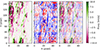 |
Fig. B.3. Simulated Doppler velocity maps representing a proxy for the effect of SPICE PSF tilt on velocities (panel (a)). Panel (b) shows the Doppler velocities obtained with SPICE for comparison. Panel (c) shows simulated velocity maps on top of Doppler maps obtained with SPICE. |
Panel (b) shows the Doppler map obtained with SPICE taken with the C III raster at 14:02:59. The proxy map serves the purpose of identifying regions at greater risk of producing an artificial signal. Figure B.3 (c) shows the proxy map imposed on top of the Doppler map and allows the location of the spine to be matched with the proxy map. From panel (c), we deduced that the spine region is sufficiently secure because it does not coincide with the high-risk areas for acquiring false signals. Consequently, these findings serve as additional evidence that supports the results obtained through forward-modeling analysis.
All Figures
|
Fig. 1. Overview of the instrument’s FoVs as viewed from the Solar Orbiter FSI in 174 Å. Overlaid on top is the HRIEUV FoV, shown by red rectangle, and the SPICE and PHI FoVs are shown by blue and green rectangles, respectively. |
| In the text | |
|
Fig. 2. First frame of the sequence of images taken by HRIEUV. The left panel shows the original movie. The right panel shows a running difference movie mimicking the panel on the left. The spine dynamics show untwisting motions propagating toward the remote footpoint denoted by the red circle in the left panel. A movie is available online. |
| In the text | |
|
Fig. 3. Magnetograms obtained with PHI HRT. Panel a shows the cropped FoV of HRIEUV imposed on top of the HRT view. The blue rectangle shows the location of the spine. Red dashed curves show identified loops used for alignment purposes. The black dashed circle shows a sunspot near the spine. Panel b shows a zoomed-in view of the feature. Panel c shows a PHI zoomed-in view alone. Red dashed circles show the footpoint at the origin of the spine and the footpoint corresponding to the remote brightening. |
| In the text | |
|
Fig. 4. Magnetic configuration of the spine and the propagating pulse. Panel a shows the sketch of magnetic structure. Courtesy of Yang et al. (2020). The purple spiral shows the propagation of an Alfvén wave. Panel b illustrates the propagation of one single Alfvén wave pulse. |
| In the text | |
|
Fig. 5. Field line rendering of the potential field in the vicinity of the null point. The background image represents the radial magnetic field saturated between −800 and 800 G; field lines are colored with the potential field magnitude, in logarithmic scale. The top-left inset shows an enlarged side-view of the null region. |
| In the text | |
|
Fig. 6. Intensity maps obtained with SPICE for four different lines starting from the cool chromosphere and incrementally increasing up to the coronal temperatures. The first row shows three consecutive frames (14:02:59, 14:14:28, and 14:25:57) for the H I Lyβ line, the second row shows intensity maps for the C III line, and the two last rows show intensity maps for the Ne VIII and Mg IX lines, correspondingly. |
| In the text | |
|
Fig. 7. Time-distance map demonstrating the propagation. Panel a shows a snapshot of the difference movie with the highlighted region (red dashed curves) that was used to create a time-distance map. Panel b shows the time-distance map where propagating material is clearly visible. Red lines represent fits to the propagating wave fronts with their annotated values of propagation velocity. |
| In the text | |
|
Fig. 8. Snapshots of running ratios plotted on top of the HRIEUV images. The white arrows represent the direction of plasma material movement. The color bar represents intervals of time used to construct the running ratio. |
| In the text | |
|
Fig. 9. Snapshots of running ratios. Panel a shows the spine, where the red rectangle highlights the area of interest. Panels b–h display zoomed-in views corresponding to different time frames starting from 14:01:40 and separated by five seconds. Points are colored according to the time, with the color bar shown at the top. |
| In the text | |
|
Fig. 10. Time-distance maps demonstrating the transverse motion. Slits used to construct time-distance maps are shown by white dashed lines (left column). Numbers denote the number of each slit. Time-distance maps were constructed from the slits taken across the spine (middle column) to show the evidence of the movement in the transverse direction. The third column shows a zoomed-in view with the points fitted to the propagating pulse. The zoomed-in view is indicated by a blue rectangle in each figure in the middle column. |
| In the text | |
|
Fig. 11. Intensity and Doppler maps obtained with the SPICE C III line for three time frames (14:02:59, 14:14:28, and 14:25:57). Panels a and b show maps for the first time frame, panels c and d are for the second, and panels e and f are for the last frame. The white rectangle in panel a shows the location of the spine. Black ellipses in panels b, d, and f show the location of a strong signal that matches the high intensity gradient in panel a. The magenta ellipse in panel b shows the location of a strong Doppler signal that does not correspond to the high intensity gradient. |
| In the text | |
|
Fig. 12. Synthesized spectral rasters obtained using forward-modeled analysis. Panel a shows the synthesized intensity, while the panels b and c show the Doppler maps (mimicking the SPICE CIII line) with and without local velocities imposed on top of the feature. The black ellipse in panel c shows the location of a strong signal that corresponds to the high intensity gradient. The magenta ellipse outlines the location that does not correspond to any intensity gradient. |
| In the text | |
|
Fig. A.1. The model of the rigid body rotation. Central lines of the feature identified in rigid body rotation are denoted by dashed black lines (panel (a)). Panel (b) depicts the velocity field imposed on top of the feature. |
| In the text | |
|
Fig. B.1. Spectra from a particular slit position in SPICE and forward-modeled data. The slit is passing through the spine region. |
| In the text | |
|
Fig. B.2. Relation between the intensity gradients along (panel (a)) and across (panel (b)) the SPICE slit with the Doppler velocities. The orange dashed lines show the ±1σ range that was excluded from the linear fit (black line). This sample was taken from the C III raster at 14:02:59. |
| In the text | |
|
Fig. B.3. Simulated Doppler velocity maps representing a proxy for the effect of SPICE PSF tilt on velocities (panel (a)). Panel (b) shows the Doppler velocities obtained with SPICE for comparison. Panel (c) shows simulated velocity maps on top of Doppler maps obtained with SPICE. |
| In the text | |
Current usage metrics show cumulative count of Article Views (full-text article views including HTML views, PDF and ePub downloads, according to the available data) and Abstracts Views on Vision4Press platform.
Data correspond to usage on the plateform after 2015. The current usage metrics is available 48-96 hours after online publication and is updated daily on week days.
Initial download of the metrics may take a while.