| Issue |
A&A
Volume 675, July 2023
Solar Orbiter First Results (Nominal Mission Phase)
|
|
|---|---|---|
| Article Number | A110 | |
| Number of page(s) | 19 | |
| Section | The Sun and the Heliosphere | |
| DOI | https://doi.org/10.1051/0004-6361/202245586 | |
| Published online | 07 July 2023 | |
First perihelion of EUI on the Solar Orbiter mission
1
Solar-Terrestrial Centre of Excellence – SIDC, Royal Observatory of Belgium, Ringlaan -3- Av. Circulaire, 1180 Brussels, Belgium
e-mail: david.berghmans@oma.be
2
Department of Mathematics, Physics and Electrical Engineering, Northumbria University, Newcastle upon Tyne NE1 8ST, UK
3
Institut d’Astrophysique Spatiale, CNRS, Univ. Paris-Sud, Université Paris-Saclay, Bât. 121, 91405 Orsay, France
4
Max Planck Institute for Solar System Research, Justus-von-Liebig-Weg 3, 37077 Göttingen, Germany
5
Physikalisch-Meteorologisches Observatorium Davos, World Radiation Center, 7260 Davos Dorf, Switzerland
6
ETH Zürich, Institute for Particle Physics and Astrophysics, Wolfgang-Pauli-Strasse 27, 8093 Zürich, Switzerland
7
European Space Agency, ESTEC, Keplerlaan 1, PO Box 299, 2200 AG Noordwijk, The Netherlands
8
UCL-Mullard Space Science Laboratory, Holmbury St. Mary, Dorking, Surrey RH5 6NT, UK
9
Southwest Research Institute, 1050 Walnut Street, Suite 300, Boulder, CO 80302, USA
10
Skobeltsyn Institute of Nuclear Physics, Moscow State University, 119992 Moscow, Russia
11
Sorbonne Université, Observatoire de Paris – PSL, École Polytechnique, Institut Polytechnique de Paris, CNRS, Laboratoire de physique des plasmas (LPP), 4 place Jussieu, 75005 Paris, France
12
Rosseland Centre for Solar Physics, University of Oslo, PO Box 1029, Blindern, 0315 Oslo, Norway
13
Laboratoire Charles Fabry, Institut d’Optique Graduate School, Université Paris-Saclay, 91127 Palaiseau Cedex, France
14
Centre Spatial de Liège, Université de Liège, Av. du Pré-Aily B29, 4031 Angleur, Belgium
15
AESTER INCOGNITO, 75008 Paris, France
16
LATMOS, CNRS – UVSQ – Sorbonne Université, 78280 Guyancourt, France
17
Centre for mathematical Plasma Astrophysics, KU Leuven, 3001 Leuven, Belgium
18
Institute of Physics, University of Maria Curie-Skłodowska, Pl. M. Curie-Skłodowskiej 5, 20-031 Lublin, Poland
Received:
30
November
2022
Accepted:
2
March
2023
Context. The Extreme Ultraviolet Imager (EUI) on board Solar Orbiter consists of three telescopes: the two High Resolution Imagers, in EUV (HRIEUV) and in Lyman-α (HRILya), and the Full Sun Imager (FSI). Solar Orbiter/EUI started its Nominal Mission Phase on 2021 November 27.
Aims. Our aim is to present the EUI images from the largest scales in the extended corona off-limb down to the smallest features at the base of the corona and chromosphere. EUI is therefore a key instrument for the connection science that is at the heart of the Solar Orbiter mission science goals.
Methods. The highest resolution on the Sun is achieved when Solar Orbiter passes through the perihelion part of its orbit. On 2022 March 26, Solar Orbiter reached, for the first time, a distance to the Sun close to 0.3 au. No other coronal EUV imager has been this close to the Sun.
Results. We review the EUI data sets obtained during the period 2022 March–April, when Solar Orbiter quickly moved from alignment with the Earth (2022 March 6), to perihelion (2022 March 26), to quadrature with the Earth (2022 March 29). We highlight the first observational results in these unique data sets and we report on the in-flight instrument performance.
Conclusions. EUI has obtained the highest resolution images ever of the solar corona in the quiet Sun and polar coronal holes. Several active regions were imaged at unprecedented cadences and sequence durations. We identify in this paper a broad range of features that require deeper studies. Both FSI and HRIEUV operated at design specifications, but HRILya suffered from performance issues near perihelion. We conclude by emphasizing the EUI open data policy and encouraging further detailed analysis of the events highlighted in this paper.
Key words: Sun: corona / Sun: chromosphere / Sun: coronal mass ejections (CMEs) / instrumentation: high angular resolution / Sun: filaments / prominences / Sun: flares
© The Authors 2023
 Open Access article, published by EDP Sciences, under the terms of the Creative Commons Attribution License (https://creativecommons.org/licenses/by/4.0), which permits unrestricted use, distribution, and reproduction in any medium, provided the original work is properly cited.
This article is published in open access under the Subscribe to Open model. Subscribe to A&A to support open access publication.
1. Introduction
The launch of the Atmospheric Imaging Assembly (AIA) on board the Solar Dynamics Observatory (SDO; Pesnell et al. 2012) in 2010 heralded the era of continuous full-disk coronal imaging at high spatial resolution. In normal mode, AIA images are produced with a cadence of 12 s at a spatial resolution of 1.5″, over a field of view (FOV) of (41′)2 (Lemen et al. 2012). Recent developments in coronal imagers have included increased FOVs and higher spatial resolution. SWAP on PROBA2 (Seaton et al. 2013; Halain et al. 2013) and SUVI on GOES (Darnel et al. 2022) have boosted observations with FOVs of (54′)2 and (53′)2, respectively. Thanks to these larger FOVs, both SWAP and SUVI image the extreme ultraviolet (EUV) structures and dynamics well beyond the AIA FOV, into what has become known as the Middle Corona (Seaton et al. 2021; West et al. 2023; Chitta et al. 2023). Meanwhile, the sounding rocket Hi-C (Kobayashi et al. 2014) pushed the limits in terms of spatial resolution. In its second successful flight (Rachmeler et al. 2019), Hi-C took (subfield) images of an active region at a cadence of 4 s and a spatial resolution better than 0.46″ (330 km on the Sun).
Solar Orbiter (Müller et al. 2020) is in a highly elliptical orbit with perihelia below 0.3 au and, in later years of the nominal mission, well out of the ecliptic, beyond 30° solar latitude. The Extreme Ultraviolet Imager (EUI; Rochus et al. 2020) on board Solar Orbiter will use this unique orbit to observe the Sun from different vantage points through three separate telescopes, imaging the outer solar atmosphere at an even higher spatial resolution than Hi-C, and over wider fields of view than SUVI and SWAP, further extending the middle corona discovery space.
The first EUI telescope, the Full Sun Imager (FSI) is a one-mirror telescope taking alternating images in the 17.4 nm and 30.4 nm passbands. For a coronal EUV imager, FSI has an unprecedentedly large FOV: (228′)2, which has a significant overlap (Auchère et al. 2020) with the Solar Orbiter coronagraph Metis (Antonucci et al. 2020). At perihelion, this FOV corresponds to (4 R⊙)2 such that the full solar disk is always seen, even at maximum offpoint (1 R⊙). This FOV is significantly wider than the (3.34 R⊙)2 of EUVI (Howard et al. 2008) or the (3.38 R⊙)2 of SWAP (Seaton et al. 2013). When at 1 au (near aphelion), this FOV corresponds to (14.3 R⊙)2 providing unique opportunities to image the Middle Corona and eruptions that transit through this region.
The other EUI telescopes are the two High Resolution Imagers (HRIs), HRIEUV and HRILya, which are two-mirror optical systems imaging through EUV and hydrogen Lyman-α passbands respectively. HRIEUV images the corona at 17.4 nm, which corresponds to the 17.4 nm channel of FSI. HRILya, which images in the Lyman-α line, shares its resonance formation process for hydrogen with the 30.4 nm channel of FSI for helium. The HRIEUV plate scale is 0.492″; the HRILya plate scale is 0.514″. At the 2022 March 26 perihelion, Solar Orbiter reached a distance of 0.323 au from the Sun, giving (single) pixel values on the Sun of (115 km)2 for HRIEUV, and (120 km)2 for HRILya. The actual spatial resolution of the telescopes is discussed in Sect. 4. Both HRI cameras are capable of operating at cadences in the 1 s range, over 2048 × 2048 pixel arrays. The HRIs image through a 17′×17′ FOV, corresponding to (1 R⊙)2, when observing at 1 au, and (0.28 R⊙)2 at perihelion.
Following its launch on 2020 February 10, Solar Orbiter spent four months in the Near Earth Commissioning Phase, followed by 17 months of Cruise Phase. During the Cruise Phase only the in situ instruments were collecting science grade data, while the remote sensing instruments were undergoing extended testing in preparation for the science phase of the mission. The Nominal Mission Phase of Solar Orbiter started on 2021 November 27. During the Nominal Mission Phase, the remote sensing instruments run a nonstop synoptic observation program interleaved three times per orbit with ten-day periods of enhanced observational activity. These periods are called Remote Sensing Windows (RSWs) and are typically scheduled at the perihelion of the orbit of Solar Orbiter and at the times of minimum and maximum latitude.
In this paper we present an overview of the unique data sets collected by EUI during the very first close perihelion RSWs, covering the period from 2022 March 2 to 2022 April 6 (Fig. 1, reproduced from the ESA Solar Orbiter website1). Compared to Earth, Solar Orbiter observed from a perspective of increasing solar longitude (i.e., east to west), and transitioned from near-alignment with Earth on 2022 March 6 to perihelion on 2022 March 26, and then in a quadrature formation with the Earth, observing the Sun above the west limb on 2022 March 29. During that period the distance to the Sun from Solar Orbiter varied from 0.32 au to 0.55 au, closer to the Sun than any coronal EUV imager before. Given the variable angle with the Earth, the variable distance to the Sun, and the constraints of the low telemetry bandwidth, the instrument operations of the remote sensing payload on Solar Orbiter was highly non-synoptic. The aim of the paper is to guide the EUI data user through the unique but very variable EUI observations that were collected in the period 2022 March 2 to April 6. In Sect. 2 we present the various EUI observation campaigns that were taken during perihelion. In Sect. 3 we give an overview of the observational highlights that were completed in these campaigns. After that, in Sect. 4, we describe for each EUI telescope the instrument performance. Finally, in Sect. 5, we give an outlook for upcoming orbits.
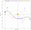 |
Fig. 1. Trajectory of Solar Orbiter in Geocentric Solar Ecliptic (GSE) coordinates in black, starting at 2021 December 27 (square). The Remote Sensing Windows (RSW) correspond to the orange, red, and blue parts of the trajectory. In this paper the period from 2022 March 02 (beginning of RSW1, orange) to 2022 April 06 (end of RSW3, blue) is covered. Perihelion occurred at the end of the RSW2 (red), around 2022 March 26. The trajectories of the ESA mission Bepi Colombo and the NASA missions STEREO-A, and Parker Solar Probe are indicated brown, green, and purple, respectively. |
2. From science goals to EUI data sets
As Solar Orbiter is a deep space non-synoptic probe, the activity scheduling of its instruments is coordinated well in advance. This is done through Solar Orbiter Observing Plans (SOOPs), which bring a group of Solar Orbiter instruments in a specific mode to target a certain science goal at appropriate times during the orbit. These science goals have been generically described in Zouganelis et al. (2020) and updates are maintained on the ESA Solar Orbiter website.
In order to document the intended purpose and context of the collected observations, we here summarize the SOOPs that the EUI instrument was involved in during the 2020 March 2 to April 6 period. Grouping the SOOPs by science target and by increasing operational complexity, we arrive at three themes: (1) observing the Middle Corona off-limb, (2) observing the building blocks of the solar atmosphere, and (3) making the connection from high-resolution on-disk observations to in situ measurements of the solar wind. The full technical details of the resulting EUI data sets can be found in Appendix A, where entries are linked to corresponding SOOP names.
2.1. Observing the off-limb Middle Corona
The first set of SOOPs focused on the off limb corona. Most of these SOOPs are led by the Solar Orbiter coronagraph Metis, which requires Sun center pointing. This makes the SOOPs operationally simpler as no last-minute pointing corrections are needed. For these SOOPs the EUI FSI images are prioritized, due to the large overlap with Metis (Auchère et al. 2020). Optional HRI images are necessarily pointed near disk center.
The aim of the L_FULL_HRES_MCAD_Coronal-He-Abundance SOOP on 2022 March 7 was to support observations during the second launch of the Herschel sounding rocket, whose first flight provided the first helium abundance maps of the solar corona (Moses et al. 2020). The abundance is deduced from the ratio of the resonantly scattered intensities of neutral hydrogen and singly ionized helium, as imaged by two coronagraphs: SCORE (Romoli et al. 2003) and HeCOR (Auchère et al. 2007). The method is model-dependent, and requires an independent knowledge of the temperature of the scattering ions. This can be constrained by simultaneous EUV observations, which was the purpose of the FSI observations at 17.4 nm. In order to minimize stray light at large distances from the solar limb, the instrument was used in coronagraph mode, with a movable disk masking direct sunlight (see Auchère et al. 2005; Rochus et al. 2020). One of the returned images is shown in Fig. 2, composited with the closest-in-time disk image taken before the campaign. The sounding rocket payload failed, but the FSI data are still very useful to study the 17.4 nm emission of the extended corona. A modulation pattern is visible, dark hexagons near the FSI vignetting cutoff, caused when the occulter is blocking part of the beam footprint on the mesh grids that support the front and focal filters (Auchère et al. 2011, 2023b). The composite EUV image allows us to link the magnetic structures on the disk (coronal holes, plumes, active regions) to magnetic field expansions in the extended corona, which always appear open, but are far from being simply radially aligned.
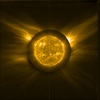 |
Fig. 2. FSI image taken in coronagraph mode (outer FOV) on 2022 March 7 at 16:00:05 UT, composited with a regular disk image (center) taken at 11:29:45 UT. The images were enhanced using the WOW algorithm (Auchère et al. 2023a) to reveal faint features (see Sect. 2.1). |
The L_FULL_HRES_HCAD_CoronalDynamics SOOP is designed to observe structures in the outer corona with the aim of linking them to the solar wind observed in situ. The SOOP was run twice, on 2022 March 22 (at 0.33 au) and March 27 (at 0.32 au) just after perihelion. Given the outer corona focus, the main contribution of EUI was through FSI observations in both wavelengths. Nevertheless, HRI images of the quiet Sun at disk center were also taken at relatively low cadence (30 s to 60 s). While these HRI images are perhaps not directly useful for the SOOP goal, they are unique observations as, given the close solar approach, they were the sharpest quiet-Sun EUV images ever taken during the first perihelion passage.
The goal of the L_FULL_HRES_HCAD_Eruption-Watch SOOP is to observe eruptive events and to contribute to the understanding of coronal mass ejections (CMEs). The SOOP was carried out in two campaigns, the first on 2022 March 22–23, and the second on 2022 March 29–30 (close to Solar Orbiter in quadrature at the west side of Earth). There was long-term monitoring with the FSI (every 6 min), while the HRIs operated in 30 min bursts.
2.2. Observing the building blocks of the on-disk solar atmosphere
A second set of SOOPs targeted various features in the on-disk solar atmosphere. These SOOPs are typically led by SPICE (SPICE Consortium 2020) and/or EUI and require pointing the spacecraft to targeted features. Pointing corrections were made a few days in advance, commanded through the so-called Pointing-Very Short Term Planning (pVSTP; Zouganelis et al. 2020) and based on low-latency FSI images that are brought to the ground as a high priority. These are typically less than a day old.
The observation of small-scale EUV brightenings in the quiet Sun was an early success of EUI (Berghmans et al. 2021). Therefore, particular attention was paid to scheduling the R_BOTH_HRES_HCAD_Nanoflares SOOP that is focused on surveying small impulsive events. There are many open questions on their origin and properties, for example whether they are also located in active regions and coronal holes. Similar events were observed in active regions by the Hi-C, but it is not clear yet if they are the same phenomenon. If this is the case, the question is whether they have the same properties everywhere. Recent work suggests that a subpopulation of the small-scale EUV brightenings does not reach the 1 MK (Dolliou et al. 2023; Huang et al. 2023). Answering these questions will help us understand, for instance, their origin and relationship with the small-scale magnetic field structuring and evolution.
The R_BOTH_HRES_HCAD_Nanoflares SOOP was scheduled several times, first near the Sun–Earth line (2022 March 7), second at an angle with the Earth of roughly 30° (2022 March 17), and finally near quadrature (2022 March 30). The spacecraft pointed alternatively to an active region and to the quiet Sun. This SOOP resulted in thousands of HRIEUV and HRILya images obtained with a cadence of usually 3 s (HRIEUV) and 5 s (HRILya) for a duration of approximately 30 min (co-temporal in both channels). The HRIEUV initial plan was to run at 2s cadence; however, the first run on 2022 March 6 failed, and the cadence was decreased to 3 s. This very high-cadence period was, in general, followed by longer periods at lower cadence. This choice came from the allocated telemetry and the need for long high-cadence temporal sequences. These campaigns were widely supported by other instruments on Solar Orbiter, but also by IRIS (De Pontieu et al. 2014), Hinode (Kosugi et al. 2007), PROBA2/LYRA (Dominique et al. 2013), and SDO/AIA. The last instrument ran in a restricted configuration (subfield, a few wavelengths) to image at an enhanced 6s cadence at four wavelengths (13.1 nm, 19.1 nm, 17.1 nm, and 30.4 nm channels).
The R_SMALL_HRES_MCAD_Polar-Observations SOOP, as described in Zouganelis et al. (2020), observes the polar magnetic fields by PHI (Solanki et al. 2020). In this early phase of the mission, however, such observations are not ideal as the spacecraft is still at low solar latitudes. Instead, the focus of the SOOP was to observe the polar coronal holes with the high-resolution imagers of EUI. Such observations are timely as polar coronal holes will soon disappear with the rising solar cycle. This SOOP was carried out three times, once when Solar Orbiter was close to the Sun–Earth line (2022 March 6), once when Solar Orbiter was close to quadrature with Earth (2022 March 30), and once more when Solar Orbiter was at roughly 120° with the Earth (2022 April 4). In the first two campaigns the solar south pole coronal hole was the target, but in the last campaign the solar north pole coronal hole was more visible. In particular, the 2022 March 30 observation of the south pole returned the best ever EUV images of a polar coronal hole as they were taken from 0.33 au with an imaging cadence of 3 s.
The R_BOTH_HRES_MCAD_Bright-Points SOOP is SPICE-focused and observes coronal bright points. This SOOP was carried out between 2022 March 8 08:10 and 14:10. During that time, FSI operated with a relatively high time cadence (5 min). HRIEUV and HRILya observed for two hours at one-minute cadence. The EUI telescopes pointed at disk center (quiet Sun), and bright points were observed.
The R_SMALL_MRES_MCAD_AR-Long-Term was carried out between 2022 March 31 and 2022 April 4. The goal was to track the decay phase of an active region. Two good candidates appeared on the solar disk a few days before the SOOP started: NOAA AR2 12975 and NOAA AR 12976 (see Fig. 3). Comparing the two regions, the leading polarity of NOAA AR 12976 provided a good target and the EUI FOV was centered on it. There was long-term monitoring with FSI (every 30 min) and burst image sequences with both HRIs, typically with a time cadence of 10 s and lasting 47 min. The regions observed during these few days produced several flares, including an M-class flare on 2022 April 2 that is discussed below.
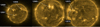 |
Fig. 3. Observed active regions on 2022 March 2 (left), March 17 (middle), and April 2 (right; see Sects. 2.2 and 2.3). |
On 2022 March 7 Solar Orbiter crossed the Sun–Earth line, at a distance of 0.49 au, allowing cross-calibration with similar Earth-bound instruments. For a complete intercomparison, a full range of scenes (quiet-Sun area, an active region, or a coronal hole) was to be targeted within the small FOV of PHI/HRT, HRIEUV, HRILya, and SPICE. However, by having Solar Orbiter point in a 5x5 pattern, these high-resolution telescopes could make a R_SMALL_HRES_MCAD_Full-Disk-Mosaic of the whole solar disk, thereby avoiding the need to guess the position of the various scenes in advance. Solar Orbiter followed the 5×5 pointing pattern from northeast (top left) to southwest (bottom right) in columns. Images in subsequent pointing positions are 10 min apart in the vertical direction and 50 min apart in the horizontal direction. To ensure a maximum overlap between image panels, the HRIEUV images were commanded to be 2368 × 2368 in size. On average, the images between dwells overlapped by ∼600 pixels. The HRIEUV telescope took high-gain and low-gain image pairs every 30 s within each dwell period, resulting in nine image pairs per pointing position. The high- and low-gain images (12 bits each) were taken 5 s apart. In processing on the ground, these images were calibrated and pixel values that were saturated in the high-gain image were replaced by the value from the low-gain image, after they were re-scaled for the different gain factor. The result is a high dynamic range image (15 bits). To create a high-resolution mosaic of the full Sun, these high dynamic range images from each dwell position were aligned and stitched together using affine image transformation making use of the spacecraft attitude information available in the source FITS files. The resulting panels were then blended together manually in photo-editing software, minimizing image artifacts in the mosaic caused by changing views in neighboring panels due to dynamic events and solar rotation. The panels were blended together preferentially in quiet-Sun areas, avoiding the faster changing active regions where possible. The final mosaic has more than 83 million pixels, making it the highest resolution image of the Sun’s full disk and corona ever taken. An interactive version of the image can be found in Kraaikamp (2022).
2.3. Making the connection from high resolution on-disk to in situ
A third set of SOOPs was implemented to find the connection between the smallest features imaged on-disk to the corresponding in situ measurements of the outflowing solar wind.
The goal of the L_SMALL_MRES_MCAD_ConnectionMosaic SOOP is to identify, with SPICE and the high-resolution imagers of EUI and PHI, the connection point on the solar disk for the solar wind observed in situ. In order to increase the probability of successfully catching the connection point, this SOOP is implemented in combination with a mosaic of spacecraft pointings. The SOOP was run twice, once when Solar Orbiter was near the Sun–Earth line (2022 March 2–3, at 0.56 au) and once when Solar Orbiter was in quadrature with Earth (2022 March 30, at 0.33 au). In the first instance the spacecraft made a mosaic of three vertically aligned pointings; in the second instance a mosaic of 3 × 2 pointings was made. Each of these pointings was maintained for several hours. It was later discovered that solar rotation was not correctly compensated for, so the EUI FOV slightly shifts over this duration. The location of the mosaics was decided a few days in advance with the help of various models and tools (Rouillard et al. 2020). During the first instance of this SOOP, EUI observed an M2 flare in the high-resolution FOV (see Sect. 3.1.9).
The L_SMALL_HRES_HCAD_Slow-Wind-Connection SOOP (Yardley et al. 2023) was designed to combine the remote-sensing and in situ capabilities of Solar Orbiter, observing the source of solar wind connected to the spacecraft and then detecting the plasma released from the Sun as it passed over the spacecraft several days later. Although the primary instruments used in the SOOP are SPICE and SWA (Owen et al. 2020), the EUI HRI observations provided high-resolution context images. Due to the need to identify where material passing over the spacecraft was originally ejected from the Sun, the SOOP coordinator relied heavily on the connectivity tool developed by IRAP (Rouillard et al. 2020) to identify the origin of the magnetic field predicted to be connected to Solar Orbiter during the observing window. For the first observing window (2022 March 3–6), this was the boundary between NOAA AR 12957 and a nearby equatorial coronal hole (Fig. 3). For the second window (2022 March 17–22), two different targets were selected due to a change in the connectivity of the spacecraft with respect to the solar magnetic field. The boundary of the southern polar coronal hole was selected as the target for the first part of the observing window, with the positive polarity of NOAA AR 12967 in the northern hemisphere selected as the target for the second part of the window.
The L_BOTH_HRES_LCAD_CH-Boundary-Expansion SOOP is similar to L_SMALL_HRES_HCAD_Slow-Wind-Connection discussed above, but it specifically aims to study coronal hole boundaries as possible sources of the slow solar wind. The SOOP was active between 2022 March 25 19:40 and 2022 March 27 00:00. FSI acquired 17.4 nm and 30.4 nm images at 10 min cadence. The quiet Sun at disk center was observed in both campaigns.
3. Observational highlights
In the previous section the EUI observations of the 2022 March 2–April 6 period were presented from a science planning perspective. Solar activity seldom follows the science plan, however, so we additionally review the actual observational highlights here that have been identified so far in the collected data. Due to the intrinsic motion of the spacecraft over the same period, its subsolar point ranged in this 35-day period only from 64° Carrington longitude in the beginning of the period to 95° Carrington longitude at the end of the period. The longitudinal angle Earth-Sun-spacecraft ranged from −8° to 122°. In what follows we use EUI Data Release 5 (Mampaey et al. 2022).
3.1. Active region dynamics
Several active regions (see Fig. 3) were observed in the HRIEUV and HRILya FOVs with imaging cadences sometimes as fast as 3 s. Below we highlight a sample of some particular dynamics.
3.1.1. Decayless kink oscillations
NOAA AR 12957 was observed first as part of the mosaic pattern of L_SMALL_MRES_MCAD_ConnectionMosaic (2022 March 2, 3) and then as part of the daily high-resolution bursts of L_SMALL_HRES_HCAD_Slow-Wind-Connection on 2022 March 3, 4, and 5. At this time Solar Orbiter was at 0.544 au from the Sun, resulting in an HRIEUV pixel footprint of 194 km on the Sun. The core of the active region showed a myriad of counter-streaming loops, some of which exhibited decayless kink oscillations (Fig. 4). This event is of particular interest due to the fact that these oscillating loops are rooted inside sunspots that are generally devoid of supergranular flows, the commonly assumed driver of such decayless kink oscillations. Moreover, these decayless oscillations were only observed during specific time intervals, although the loop environment remained quite similar throughout. Further details of the magnetic configuration of those loop footpoints, and of the existence of other possible wave drivers are presented in Mandal et al. (2022).
 |
Fig. 4. Example of decayless kink waves observed in AR12957 on 2022 March 04. Panel b shows a magnified image of the loops in panel a. The boxes S1 to S3 indicate the slits along which the temporal evolution is shown in the form of space-time diagrams in panels c to e. To enhance the appearance of the oscillating threads in these space-time diagrams, a smooth version of the map (boxcar-smoothed in the vertical direction) is subtracted from each original map. The black lines represent fits for the oscillation of the loops (see Sect. 3.1.1 for details). |
3.1.2. Braiding loops
As a part of the R_BOTH_HRES_HCAD_Nanoflares SOOP on 2022 March 17, HRIEUV observed active region AR12965 at a cadence of 3 s. These are among the highest cadence EUV images of an active region ever observed (e.g., the HI-C 2.1 sounding rocket achieved 4.4s cadence; Rachmeler et al. 2019). During this period, Solar Orbiter was at a distance of 0.38 au. Thus the two-pixel footprint of HRIEUV was about 270 km on the Sun. An overview of the observed active region is displayed in Fig. 5a. The high-resolution high-cadence observations of this active region revealed a number of impulsive EUV brightenings on timescales of a few minutes or less. A closer look at some of the brightenings revealed that they are associated with untangling of braided coronal strands or loops. Most of these events are observed in shorter low-lying loop features. HRIEUV also observed untangling of coronal braids in a more conventional loop system. A sequence of this untangling of braided loops is shown in Figs. 5b–j. More details of examples of braided structures observed by HRIEUV and the implications for coronal heating are discussed in Chitta et al. (2022).
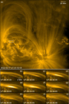 |
Fig. 5. Example of a relaxation of braided coronal loops observed on 2022 March 17. Panels b to j display magnified image of the loop in panel a, (white box) and show the evolution of the untangling within the loop (see Sect. 3.1.2 for details). |
3.1.3. Highly dynamic cooler loops
The region of interest of R_SMALL_MRES_MCAD_AR-Long-Term on 2022 April 1 was on the east limb of the Sun from the vantage point of Solar Orbiter, which means that the same region appeared in the western hemisphere from the viewpoint of Earth. Figure 6a shows the full FOV of HRIEUV, with NOAA AR 12975 on the western side and NOAA AR 12976 on the eastern side. In addition to imaging instances of coronal braids in low-lying loop systems in both these active regions (see discussion in Chitta et al. 2022), HRIEUV captured a highly dynamical system of cooler loops that appear darker in EUV due to absorption. These dynamic loops were observed in the core of AR12975 (see white box in Fig. 6). These are likely related to chromospheric arch-filament systems associated with emerging flux regions (van Driel-Gesztelyi & Green 2015). Individual strands or loops within this system exhibited intermittent brightenings in EUV. In addition, there are also repeated compact brightenings at one end of this feature. The morphology of these compact EUV brightenings appear similar to the transition region ultraviolet bursts that are often observed in emerging flux regions (Young et al. 2018). The evolution of this region over a period of one hour is displayed in a sequence of images in Figs. 6b–j.
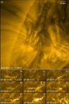 |
Fig. 6. Example of a highly dynamic cool loop system in the core of active region AR12975 observed by HRIEUV on 2022 April 1 (see Sect. 3.1.3). |
3.1.4. Brightening on border of dark material
During the R_SMALL_MRES_MCAD_AR-Long-Term SOOP on 2022 April 1, HRIEUV observed brightening events at the top of dark jet-like structures. The angular separation between the Earth and Solar Orbiter was 104°, which allowed the simultaneous observation from SDO/AIA in near-quadrature. Solar Orbiter was 0.35 au from the Sun, resulting in a spatial resolution of HRIEUV images (two pixels in size) of 248 km. The dark jet-like structures appear to be the so-called light walls (Hou et al. 2016) or fan-shaped jets (Robustini et al. 2016), which are field-aligned long chromospheric jets thought to be produced by magnetic reconnection in the photosphere (Bharti 2015; Bai et al. 2019). Two kinds of brightening events can be distinguished (see time–distance map in Fig. 7). The first kind is continuously present at the chromosphere-corona interface of the jets and is seen to oscillate up and down with a ballistic motion, strongly suggesting that this corresponds to the upward motion of the transition region observed by HRIEUV (17.4 nm). Its remarkable thinness (as small as 200 km or less) and strong brightness is probably due in part to the passage from high to low density and cool to hot plasma, to which HRIEUV is particularly sensitive. The second kind of brightening is far more impulsive, with lifetimes on the order of 10 s or less, and appears on top of the first kind as perturbances propagating upward at speeds of ≈100 km s−1. Both brightening events are therefore likely due to slow mode shocks generated from the reconnection events lower down, first propagating in the chromosphere and then into the corona at the tube speed. The second kind is seen to originate when the dark structure is at the lower end of the oscillation range, as expected from chromospheric shocks leading to spicule-like events (Heggland et al. 2007, 2011).
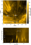 |
Fig. 7. HRIEUV observations of the brightening on a border of dark material in an active region on 2022 April 1. The white arrows in the top panel mark the brightening location. The bottom panel shows a time–distance map along one of the jets observed propagating from the bright structure. Two kinds of brightening events can be seen: the bright edge of the dark structure oscillating up and down, and jets propagating upward (both indicated by the arrows; see Sect. 3.1.4). |
3.1.5. Coronal rain
Coronal rain appears ubiquitous on-disk in AR NOAA 2974 and 2976 observed on 2022 March 30, April 1 and 2 (see Fig. 8). In HRIEUV, coronal rain can be clearly distinguished in EUV absorption by its dynamics (with velocities close to 100 km s−1 in the plane of the sky) and its clumpy and multi-stranded morphology (Antolin et al. 2015; Antolin 2020). At the spatial resolution of ≈250 km, individual coronal rain clumps only a few pixels wide can be observed. Their morphology is strongly reminiscent of Hα high-resolution observations (Antolin & Rouppe van der Voort 2012), a similarity that has been predicted, but so far only observed at larger loop scales (Anzer & Heinzel 2005; Yang et al. 2021). Coronal rain showers (composed of clumps) can be observed in loop bundles rooted to moss (Berger et al. 1999), but both clumps and showers (despite the large shower widths above 10 Mm) appear mostly unresolved in AIA passbands. This picture therefore constitutes a major difference to previous EUV observations of active regions. The on-disk observation at high resolution provides a connection to the chromosphere (and photosphere with PHI), thus providing a unique insight into the heating events at the footpoints that lead to thermal non-equilibrium and instability associated with this phenomenon (Antolin & Froment 2022). A full paper reporting coronal rain observed with HRIEUV is available in Antolin et al. (2023).
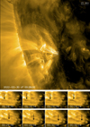 |
Fig. 8. AR NOAA 2974 observed on 2022 March 30 by HRIEUV at the southeast limb. Top: Full FOV; the solid white curves follow several trajectories of coronal rain clumps seen in EUV absorption. Bottom panels: Snapshots at various instances of a coronal rain shower, corresponding to the small white rectangle shown in the top panel. The black arrows indicate the head of the coronal rain shower (see Sect. 3.1.5). |
3.1.6. Hints of torsional Alfvén waves in twisted coronal loops
In AR NOAA 2975 observed on 2022 April 2, twisted intertwined coronal strands can be observed in the plane of the sky, appearing and disappearing on a timescale of 5 − 10 min. The strands disappear by the end of the sequence with hints of untwisting, ending in coronal rain falling onto bright footpoints rooted in moss. The entire event is strongly reminiscent of the coronal loop model of Díaz-Suárez & Soler (2021), in which torsional Alfvén waves propagate along a twisted flux tube. The radially varying magnetic field due to the twist provides an Alfvén continuum that allows phase mixing to happen. The Kelvin-Helmholtz instability is then generated due to the velocity shear at the phase mixing layers, which leads to compression of the plasma and the generation of coronal strands that follow the twisted flux tube (a process also observed for kink waves; Antolin et al. 2014). The timescale of appearance or disappearance of strands, their morphology, and change in orientation during the oscillation is seen to match that observed in this event with HRIEUV (see Fig. 9).
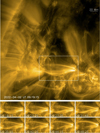 |
Fig. 9. AR NOAA 2975 observed on 2022 April 2 by HRIEUV near the northeast limb. Top: The solid white rectangle shows a twisted coronal loop where hints of torsional Alfvén waves may be observed. Bottom panels: Snapshots over 30 min evolution of the loop observed in the field of view corresponding to the white rectangle where a change in orientation of the twisted EUV strands can be seen (see Sect. 3.1.6) |
3.1.7. Large-scale reconfiguration of coronal loop substructure
In AR NOAA 2975 observed on 2022 April 1, a large-scale loop bundle rooted in moss is composed of various strands. Without the presence of any flare in the vicinity, the strands undergo a coherent reconfiguration similar to contraction following a flare (see Fig. 10). The strands also exhibit continuous kink motions during the global contracting motion. The overall event is accompanied by coronal rain.
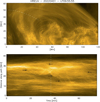 |
Fig. 10. Reconfiguration of loops substructure. Top: Subfield of the 2022 April 1 data set observed by HRIEUV (located in the bottom right of Fig. 6). A loop bundle is seen (inverted in this figure in order to have the apex on top), where a large-scale reconfiguration is observed. Bottom: Time–distance plot across the apex of the loop (dashed white curve in top panel), revealing a downward (inward) motion of many loops (akin to contraction), indicated by the black arrows, accompanied by transverse oscillations. The time of the snapshot in the top panel corresponds to the vertical white dashed line (see Sect. 3.1.7). |
3.1.8. Coronal strands associated with coronal rain
In AR NOAA 2975 observed on 2022 April 1, coronal strands rooted in moss are observed to appear and disappear on a short timescale of tens of minutes. Unlike usual coronal strands, these appear first near the loop apex and are seen to extend dynamically toward the footpoints in a flow-like manner. This is followed by localized dark or bright features at the loop apex with the appearance and dynamics of coronal rain (see Fig. 11). The entire event strongly resembles the 2.5D MHD numerical modeling of coronal rain by Antolin et al. (2022).
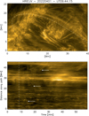 |
Fig. 11. Coronal strands associated with coronal rain. Top: Subfield of the 2022 April 1 data set observed by HRIEUV (located on the right of Fig. 6a). A loop bundle rooted on moss is seen composed of various strands. The strands appear first near the apex and exhibit bright and dark flows with dynamics characteristic of coronal rain. Bottom: Time–distance plot along one of the observed strands (dashed white curve in top panel). The fuzzy brightening events along the middle of the strand are followed by bright or dark flows toward either footpoint of the strand (indicated by the white arrows). The time of the snapshot in the top panel corresponds to the vertical white dashed line (see Sect. 3.1.8). |
3.1.9. M2 flare: 2022 March 2
The chances to observe flares in the small FOVs of the HRIs, which are only operated over a small fraction of an orbit, are not large. Nevertheless, on 2022 March 2, during the mosaic pattern of L_SMALL_HRES_HCAD_Slow-Wind-Connection, an M2 flare was observed in active region NOAA 12958 by HRIEUV and HRILya (Fig. 12). This is the largest flare seen to date in the HRI subfields. Since the HRIs FOV only covered the lower part of this active region, in Fig. 12 we also used AIA 17.1 nm and 30.4 nm images to show the context of the evolution of the entire active region.
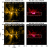 |
Fig. 12. M2 flare on 2022 March 2. Left panels: Combination of AIA 17.1 nm images and HRIEUV 17.4 nm, the latter shown within the white box (only a few seconds apart). Right panels: Same, but for the combination of AIA 30.4 nm and HRILya images. The bottom row is taken 10 min later than the top row images. The white boxes delineate the boundaries of the areas showing data from EUI-HRIs (see Sect. 3.1.9). |
Solar Orbiter was at 0.55 au from the Sun, meaning that the spatial resolution of the HRIEUV images (two pixel size) is 397 km. The imaging cadence was unfortunately only 2 min. Figure 12 shows the two ribbons shortly before the flare peaked at 17:34 and HRIEUV saturated with a front filter diffraction pattern. The HRIEUV images show several small-scale brightenings during the pre-flare time. Views from HRIEUV and HRILya are shown within the white boxes in Fig. 12. Thanks to the high resolution of HRIEUV (left panels), we can observe in detail the brightening structures in this active region, such as the double J-shaped brightening in the core region. In the right panels, the lower resolution and the saturated signal of the HRILya images only allow us to distinguish the outline of the brightening structures. After the peak time, some brightenings can be found at the upper edge of the HRIs FOV appearing at the source region and propagating from west to east, forming a long thin bright band of several dozen Mm, as shown in the right panels. Flare loops are clearly visible in the HRIEUV image, while the flare ribbons (and flare-driven rain) are visible as two parallel bright structures in the HRILya image.
Figure 13 shows that the temporal variation of the intensities observed by HRIEUV and HRILya are in qualitative agreement with comparable observations by SDO/AIA and GOES/LYA. The HRIEUV intensity corresponds well with the SDO/AIA 17.1 nm and 30.4 nm, only the emission observed in SDO/AIA 9.4 nm occurs a few minutes after the rest of the presented lines. The HRILya and GOES/LYA intensity curves corresponds well too.
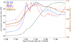 |
Fig. 13. Temporal evolution of intensity of the M2 flare on 2022 March 2. The color-coded lines present average intensities at the flare region observed with HRIEUV, HRILya, SDO/AIA, and GOES (see Sect. 3.1.9). |
3.2. Quiet-Sun features
In the current phase of the solar cycle, most active regions appear beyond 15° solar latitude north or south, meaning that whenever Solar Orbiter was not off-pointed away from disk center, the HRIs had the quiet Sun in the FOV. Below we present a small sample of quiet-Sun features and events that illustrate the quality of the obtained data.
3.2.1. Small-scale EUV brightenings
On 2022 March 26 Solar Orbiter reached its first perihelion during the Nominal Mission Phase at a distance of 0.323 au from the Sun. The HRIEUV observations closest to perihelion were taken on March 27, starting at 19:40 (distance 0.324 au), and were part of the L_FULL_HRES_HCAD_Coronal-Dynamics SOOP. On this day HRIEUV had a pixel footprint on the sun of (115 km)2.
Small EUV brightenings observed by HRIEUV, also known as campfires, were first identified by Berghmans et al. (2021) in data taken at 0.556 au. The observed campfires were typically elongated structures from 0.2 Mm to 4 Mm with aspect ratios between 1 and 5. In Fig. 14 we show a subfield, particularly rich in campfires, taken on 2022 March 27 at a distance of 0.324 au from the Sun. The 2022 March 27 L_FULL_HRES_HCAD_Coronal-Dynamics data set has a cadence of 1 min, but several of the R_BOTH_HRES_HCAD_Nanoflares data sets have cadences as short as 3 s. The visually identified sample of campfires in Fig. 14 appear somewhat smaller (none is larger than 2 Mm), but this needs to be confirmed by objective algorithmic detection.
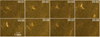 |
Fig. 14. Examples of a group of campfires observed near perihelion on 2022 March 27 (see Sect. 3.2.1). |
Figure 15 shows an example of a particularly long and slender campfire, and demonstrates that loop-like features are present in the quiet Sun with a width on the order of 200 km. It also demonstrates that the spatial resolution of HRIEUV is pixel-limited.
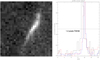 |
Fig. 15. A long and slender campfire observed on 2022 March 27. Left: Calibrated images (L2) with the original sensor pixelization; each pixel corresponds to (115 km)2 on the sun. Right: Various cross-cuts through the campfire demonstrating that the FWHM of the feature is 1−2 pixels (see Sect. 3.2.1). |
3.2.2. EUV network flares
At larger scales than campfires (≳10 Mm), flare-like brightenings are frequently seen in the quiet Sun. Figure 16 (top right) shows the location of four such flare-like brightenings in a typical quiet-Sun observed by HRIEUV on March 27–28. The time evolution of the fourth event is shown in Fig. 17 with corresponding SDO/AIA 17.1 nm imagery in quadrature showing the off-limb evolution. In X-rays these events have been called network flares Krucker et al. (1997), Attie et al. (2016). The HRIEUV extreme high-resolution EUV images of the quiet Sun confirm that these brightenings do indeed show many of the usual flare attributes, such as pre-flare sigmoids, dimmings, ribbons, and post-flare loops. For some of them, in Fig. 17 for example, we can also confirm jets and filament eruptions, making them candidate sites for “mini” CMEs Innes et al. (2009), Sterling et al. (2015).
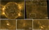 |
Fig. 16. Extreme UV network flares observed in the quiet Sun. The top left panel shows an FSI 17.4 nm image; the white rectangle indicates the magnified HRIEUV FOV shown in the top right panel. In this HRIEUV image, taken at a time without network flares, the locations of four network flares are indicated. Three of these network flares are shown in the bottom row of the figure. The fourth event is shown in Fig. 17. The HRIEUV pixels correspond to (115 km)2 on the Sun (see Sect. 3.2.2). |
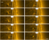 |
Fig. 17. Time evolution of an EUV network flare seen by HRIEUV on 2022 March 28 at 17.4 nm (left) near disk center and by SDO/AIA 17.1 nm near the limb. This event corresponds to location 4 in the top right panel of Fig. 16. The off-limb data confirm the eruptive character of this EUV network flare (see Sect. 3.2.2). |
3.2.3. Polar coronal holes
Fine-scale structure and dynamics of coronal holes is of particular interest for studies of the fast solar wind origin (e.g., Cirtain et al. 2007; Poletto 2015). Due to the progression of the ascending phase of the solar cycle, polar coronal holes were shrinking in 2022, so it was important to observe these structures at high spatio-temporal resolution early in the Solar Orbiter mission. During the first perihelion passage in 2022, this was done on three occasions: March 6, March 30, and April 4–5. The R_SMALL_HRES_MCAD_Polar-Observations SOOP was used (see Table A.1).
On March 30 Solar Orbiter was situated at a distance of 0.33 au from the Sun, and HRIEUV reached a two-pixel spatial resolution of around 240 km. This was the highest ever spatial resolution reached in coronal hole observations. An excellent cadence of 3 s allowed numerous dynamic fine-scale structures to be observed in the south polar coronal hole (see Fig. 18), including bright points, plumes, plumelets, jetlets, and jets (Chitta et al. 2022). Numerous campfires were visible in the adjacent quiet-Sun area.
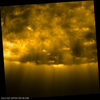 |
Fig. 18. South polar coronal hole imaged by HRIEUV on 2022 March 30 (see Sect. 3.2.3). Solar north is up; west is to the right. |
Similar data sets were taken for the north polar coronal hole on March 6 and April 4–5, when the distance from the spacecraft to the Sun was 0.5 au and 0.37 au respectively (Table A.1). The HRIEUV spatial resolution of around 270 km was reached on April 4. Seven HRIEUV images were taken at the very high cadence of 2 s on March 6, although the typical cadence was 30 s in both data sets.
3.2.4. Observations of filaments and prominences
The first perihelion passage of Solar Orbiter also permitted EUI to take close-up observations of filaments and prominences at high cadence and spatial resolution. On the disk the width of their core fine structure was resolved by HRIEUV down to the limit of the Hα instrument resolution (≈0.2″). In Hα the threads have a width distribution centered at 0.3″, which means ≈225 km on the Sun (for a review of the observations see Parenti 2014). Figure 19 shows some example of filaments seen mostly in absorption by HRIEUV. Similar absorption features are also observed by HRIEUV in coronal rain events (see Sect. 3.1.5). The top left panel shows a filament that was followed for about half an hour on 2022 March 18 at 10:30UT at a cadence of 5 s, allowing us to detect fast intensity variation on small scales along and across the structure. Full-Sun images show local activity on 2022 March 17 that led to the formation of the filament and the opening of a small coronal hole. The merging of the polar coronal hole and the dimming region formed by the eruption of the filament is discussed in Ngampoopun et al. (2023).
The second panel in the top row of Fig. 19 shows a filament close to the limb that was observed during the Full Disk Mosaic campaign on 2022 March 7 (see Sect. 2.2). Both the on-disk and of- disk part of the filament shows a complex fine structure, highlighted by dark and bright alternating wavy shaped features. During the same campaign, we also observed the prominence shown at the bottom left. This has a tornado-like shape, with thin bright and dark threads and a bright extension at the base of the coronal cavity. These observations are very promising for future quiescent prominence and filament studies as they provide elements to derive the fine-scale morphology, and characterize the dynamics from possible injected plasma and waves activity. The bottom right panel shows part of an AR filament observed on 2022 March 30. During the 30 min HRIEUV high-cadence sequence, the filament was quite active, with brightenings in threads and fine dark features levitating above the main dark body. The cadence of 3–5 s that was chosen for all the sequences shown in Fig. 19 appears to be adequate for studying the dynamics on such small scales.
3.3. Eruptions
Due to varying distance to the Sun, the FSI FOV (from disk center to edge) changed from 4 R⊙ on 2022 March 2, to 2.3 R⊙ at perihelion, and back to 2.8 R⊙ on 2022 April 6. This large FOV, unprecedented for an EUV imaging telescope, allowed us to monitor the early evolution of eruptions. Table 1 lists the approximate starting time, the shape, and the greatest height reached by the eruptions observed by FSI during the period. Some example prominence eruptions are shown in Fig. 20. They appear in a multitude of shapes (surge-like, loop-like, curled-like), and have different kinematic behavior, from slow rising to fast eruptions. In the following subsections we highlight a number of eruptions with particularly good coverage by other instruments or with space weather relevance.
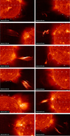 |
Fig. 20. Mosaic of prominence eruptions observed by FSI in the 30.4 nm passband in 2022 March. The “enhance off-limb” functionality of JHelioviewer (Müller et al. 2017) was used when creating these graphics (see Sects. 3.3 and 3.3.3). |
Eruptions observed by FSI between 2022 March 2 and 2022 April 6.
3.3.1. C2.8 flare: 2022 March 10
The C2.8 flare from active region NOAA 12962 on 2022 March 10 (GOES X-ray peak at 20:33) was observed by FSI as a classical two-ribbon flare, and later a post-flare arcade, with a cadence of 10 min in the 304 channel and 30 min in the 174 channel (see Fig. 21). It was also observed by the Spectrometer Telescope for Imaging X-rays (STIX; Krucker et al. 2020) and the Energetic Particle Detector (EPD; Rodríguez-Pacheco et al. 2020) on Solar Orbiter. The Earth was separated by 7.8° from Solar Orbiter. From the Earth’s perspective the flare was near the central meridian and associated with a partial halo CME that eventually led to a moderate geomagnetic storm (Kp = 6) on March 13 and 14. The evolution of the CME shock and its effect on ion acceleration was studied by Walker et al. (in prep.).
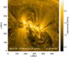 |
Fig. 21. FSI observations in the 17.4 nm passband of the C2.8 flare on 2022 March 10 (see Sect. 3.3.1). The images present the arcades of the post-flare loops. |
3.3.2. Limb CME: 2022 March 21
Starting at around 05:30 UT on 2022 March 21, an eruption was observed by FSI at the SW limb (see Fig. 22) that led to a partial halo CME observed from the Earth. The CME was associated with a Type II radio burst (measured by the Radio and Plasma Waves instrument (RPW; Maksimovic et al. 2020), with X-ray emission (observed by STIX) and with a wide SEP event measured by EPD, the Solar and Heliospheric Observatory (SOHO), and the Solar Terrestrial Relations Observatory (STEREO-A; 34° to the east of the Earth). Solar Orbiter was at 0.34 au from the Sun, and 44° west of the Sun–Earth line. The source location of the CME was located close to the west limb as seen from Solar Orbiter, at least partially occulted. The CME was fast, with speeds above 1000 km s−1. At that time EUI was executing the Slow-Wind-Connection SOOP and was observing in the 30.4 nm passband of FSI with a cadence of 30 min and in the 17.4 nm passband of FSI with 10 min cadence. A time sequence of the eruption can be seen in Fig. 22.
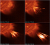 |
Fig. 22. Time sequence of the eruption on 2022 March 21, as seen by FSI in the 30.4 nm passband. The “enhance off-limb” functionality of JHelioviewer (Müller et al. 2017) was used when creating these graphics (see Sect. 3.3.2). |
3.3.3. East limb eruption: 2022 March 30
On 2022 March 30, at around 14:00 UT, FSI observed in the 30.4 nm channel a prominence erupting at the east limb (see lower left panel of Fig. 20) which was observed by SolOHI (Howard et al. 2020). Prominence material was still visible in the FSI FOV at around 20:30 UT. At around 17:30 a flare was observed on the disk (N15W30 Stonyhurst coordinates) and a bright loop was visible off-limb overlapping with the prominence, but not disturbing its evolution. This indicates that the prominence was situated far away from the flare. The SDO/AIA304 and STEREO-A/EUVI304 (Howard et al. 2008) movies show an extended filament erupting at the east of the flare. In the 17.4 nm passband, FSI observed faint material erupting at around 14:00 at the east limb followed by a big dimming off-limb at around 17:30. Material moving out is still present at 20:50. A large EUV wave was observed on-disk. The eruption was associated with a flux-rope like coronal mass ejection observed by STEREO-A/COR2 and SOHO/LASCO-C2 (Brueckner et al. 1995) coronagraphs at west limb at 18:23 and 18:12, respectively.
3.3.4. Northeast limb eruption: 2022 April 2
On 2022 April 2, FSI observed in the 30.4 nm channel a filament erupting at the NE limb (as seen from Solar Orbiter) between 13:00 and 13:30 UT. It was associated with an M3.9-class flare. The event was also captured by several other remote-sensing instruments on Solar Orbiter such as SPICE, STIX, and SoloHI. Interestingly, the erupting filament was also monitored a few days prior and during its eruption by Earth-based assets such as Solar Dynamics Observatory, IRIS, and Hinode. Its position from the Sun–Earth line was N12W68. The flare recorded by GOES soft-X ray observations indicates a start at 12:56:00, with a peak at 13:55:00 and followed by a long duration event.
This event is particularly interesting for several reasons. First, the large coverage available with different instruments allows us to follow the pre-flare phase, during which the filament slowly rises and pushes overlying coronal arcades away, as modeled in 3D numerical simulations of eruptive flares. This may be linked to the observed large-scale reconfiguration reported in Sect. 3.1.7. Second, Doppler velocity and intensity changes in several lines are reported between the upper chromosphere and transition regions (SPICE diagnostics) and in coronal lines (Hinode/EIS diagnostics) with different viewpoints. This is the first time that such an event ha been seen stereoscopically with different spectrometers. Finally, the extended coverage, from spectroscopy to EUV and X-Ray imaging, allows us to understand the evolution of the magnetic field changes during the different phases of the flare. A dedicated study of this event is available in Janvier et al. (2023) and in Ho et al. (in prep.).
4. Instrument performance at perihelion
The pre-flight instrument characterization is discussed in telescope specific papers in this issue (Auchère & EUI consortium partners, in prep.; Aznar Cuadrado & EUI consortium partners, in prep.; Gissot & EUI consortium partners, in prep.). The period around the 2022 March 27 perihelion was the first time the instrument was operated in the environment for which it was primarily designed. In this section we review how the instrument was operated technically and the resulting performance. Overall, FSI and HRIEUV performed largely nominally, while HRILya suffered from a temporary degradation in throughput and resolution (see below).
4.1. Sensors
The three EUI telescopes share the same CMOS sensor design (Rochus et al. 2020). The sensors consist of two parts, each of 1536 × 3072 pixels, stitched together as a 3072 × 3072 array. The HRI sensors are used subfielded to 2048 × 2048 pixels. Careful inspection reveals that the stitching line remains visible in all three telescopes, but most noticeably in HRILya (see Fig. 25c at x = 180 Mm).
Each pixel has a high-gain and low-gain read-out which can be brought to the ground independently or selected per pixel per intensity threshold. Onboard electronics then re-scales the high-gain and low-gain signals from different pixels into one coherent intensity range over all pixels in a “recombined” image. In the 2022 March–April period, FSI and HRIEUV were nominally operated in the combined gain mode, resulting in 15-bit images (an intensity range in Level 1 files of 0–32767 DN for FSI and 0–25600 DN for HRIEUV). The selection threshold between low-gain and high-gain read-out happens near a Level 1 intensity level of 1097 DN for FSI and 1118 DN for HRIEUV. This transition is weakly visible in the FSI and HRIEUV images as a band of enhanced noise, which is to be expected given the different photon statistics in the low-gain and high-gain read-out channels. In contrast, HRILya was operated exclusively in low-gain read-out resulting in 12-bit images (an intensity range of 0–4095 DN in the Level 1 image files) and do not show such a transition.
Other sensor artifacts affecting FSI are dark vertical bands, in very faint areas, aligned with the brightest on-disk features. This effect is assumed to be caused by saturation of the high-gain read-out of pixels in the same column and is still under investigation. A post-processing semi-empirical fix is being developed.
4.2. Onboard processing
The EUI is equipped with software-controlled onboard calibration electronics electronics for pixel-wise correction of the images for offset and flat-field correction before compression. For FSI, pre-flight offset and flat-field maps are available on board and have been applied until 2022 March 16 when it was discovered that the flat-field map was not applied correctly. Correction for the flat field was turned off at this time and subsequent FSI images only have the offset map applied.
For HRIEUV, only a synthetic four-column pattern is subtracted that mimics the observed offset. For HRILya no onboard correction is applied.
Despite the close solar proximity, radiation hits on the sensors were very limited and the onboard cosmic ray corrector was therefore not employed. Enhanced radiation hits were observed, for example following the 2022 March 21 event (see Sect. 3.3.2).
4.3. Image resolution
During commissioning, the full width at half maximum (FWHM) of the FSI point spread function (PSF) was estimated to be 1.5 pixels, or 6.66″. As shown by Fig. 23, there is no sign of change so far. At closest approach (i.e., at 0.3 au) this corresponds to a resolution of 2.5″ (two pixels) as seen from 1 au, similar to that of STEREO/EUVI (2.4″, Wülser et al. 2007).
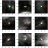 |
Fig. 23. Enlargements of selected compact features observed by FSI at 17.4 nm on 2022 March 7 at 06:20:30 UT. Assuming that the sources are unresolved, the green and red profiles (horizontal and vertical, respectively) indicate a FWHM width of the effective PSF of 1.5 pixels (see Sect. 4.3). |
The excellent resolving quality of HRIEUV was confirmed during perihelion through identification of point-like features (Fig. 24), and slender features (Fig. 15), with a FWHM width of about 1.5 pixels. This is consistent with the spatial resolution of the HRIEUV telescope being equal to the Nyquist sampling limit of 2 pixels, 2 × 0.492″. At perihelion just inside 0.3 au this corresponds to about 2 × 100 km on the Sun.
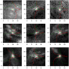 |
Fig. 24. Enlargements of selected compact features observed by HRIEUV on 2022 March 7 at 00:41:55 UT. Assuming that the sources are unresolved, the green and red profiles (horizontal and vertical, respectively) indicate a FWHM width of the effective PSF of 1.5 pixels (see Sect. 4.3). |
From the beginning of the mission, the HRILya spatial resolution was found to be lower than expected, with a first estimate placing it at around 3″ (see Berghmans et al. 2021). However, during the perihelion approach of Solar Orbiter the telescope showed a further substantial degradation of spatial resolution, contrast, and throughput. Figure 25 shows three images of quiet-Sun regions taken on 2022 March 8 (where Solar Orbiter was at a distance to the Sun of 0.49 au), March 22 (at 0.33 au), and March 30 (at 0.34 au). All targets were selected to be near disk center. The loss in performance can be clearly seen in panels (b) and (c), immediately before and after the closest approach to the Sun on 2022 March 26 (at 0.32 au). Most obvious is the resolution degradation, which may be a result of a heat effect on the entrance filter of the HRILya telescope. In addition, as Solar Orbiter approaches the Sun, both the contrast and throughput degrade by approximately 37% with respect to data taken before perihelion (around mid-February 2022), and these recover slowly after perihelion passage.
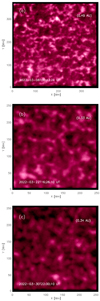 |
Fig. 25. HRILya observations of a set of quiet-Sun regions located near disk center, obtained on 2022 March 8 (panel a), 2022 March 22 (panel b), and 2022 March 30 (panel c; see Sect. 4.3). |
4.4. Filters and light leaks
The reasons for the observed overall loss of performance of HRILya during perihelion passage are currently under investigation. Experience from ground testing of the entrance filter with heating to 200 °C has revealed a nonlinear decline of its transmission of up to 40% as a function of temperature. Part of the loss of the channel’s throughput may be associated with the temperature dependency of the filter. Consistent with this, some throughput and resolution recovery was observed farther from the Sun, on 2022 June 12, which was the first HRILya observations after 2022 April. A full assessment of the evolution of throughput since launch and of its comparison with the expectations from ground calibration will be the subject of a separate publication.
In contrast to HRILya, the EUV channels may be affected by light leaks. Two issues are known to affect the FSI filters. The first is a faint light leak, likely caused by a pinhole in the front filter, that affects the images from both channels. Due to the specific design of FSI, its visibility depends on the distance to the Sun and pointing of the spacecraft. There is no quantitative correction for this yet. This has no impact for morphological studies, but care must be taken for photo-metric analysis off-disk. The second issue is a very faint light-leak, invisible in regular images, that affects the 30.4 nm data taken in coronagraph mode. Its origin is still unknown, but only a small number of images are affected.
4.5. Pointing error and jitter
The pointing information in the World Coordinate System (WCS) keywords of the EUI Level 1 FITS files are based on the as-flown Solar Orbiter spacecraft kernels. As such, these keywords capture most of the Solar Orbiter pointing instabilities, but unfortunately not all. Even after correcting for the known pointing variation, occasional jitter remains visible from image to image (as well as slower trends) in high-cadence HRIEUV sequences. However, in general the HRIEUV images do not seem to be affected much by jitter blurring.
For the FSI images, where the solar limb is always visible, the WCS pointing keywords are updated in the EUI Level 2 FITS files with much more precise information from a procedure that fits a circle to the solar limb. This is unfortunately not possible for HRIEUV and HRILya image sequences and the data user is advised to use alignment methods to remove the remaining jitter.
5. Conclusions
During the Solar Orbiter perihelion passage of 2022 March 26, and in the weeks before and after, EUI collected more than 35000 images. Solar Orbiter reached a distance to the Sun as low as 0.32 au, closer to the Sun than any other coronal imager. Both FSI and HRIEUV operated at design specifications during the perihelion passage, but HRILya suffered from an unexpected (but reversible) performance degradation near perihelion that needs to be studied further.
EUI has achieved the highest resolution images ever of the solar corona in the quiet Sun and polar coronal holes. Ubiquitous EUV brightenings (also known as campfires) and small-scale jets were recovered down to the resolution limit of HRIEUV of about 200 km on the solar surface. These smallest features require further investigation to determine their relevance to the heating of the corona and the powering of the solar wind.
Whereas the Hi-C sounding rocket (Kobayashi et al. 2014; Rachmeler et al. 2019) achieved comparable resolution in active regions, HRIEUV imaged active regions at much longer sequence durations (hours) at high cadence (3 s). Known phenomena such as coronal braiding, decayless oscillations, coronal rain, and flaring activity were observed in unprecedented detail.
The highest resolution full-disk image ever was constructed as a mosaic of 25 high-resolution images. Together with the PHI and SPICE instruments on board Solar Orbiter, this full-disk mosaic will be repeated twice per year when Solar Orbiter crosses a distance of 0.5 au from the Earth.
Meanwhile, the big novelty of FSI, namely its very extended FOV, allowed the imaging of off-limb eruptions farther away from the Sun than ever before. In particular prominence eruptions show a bewildering variety of structural appearances.
Future perihelia will go another 10% closer to the Sun, to a distance of 0.29 au from the Sun, and as the mission progresses, Solar Orbiter/EUI will also observe from increasing solar latitudes. Many of the SOOPs and EUI observations presented in this paper will be repeated from these upcoming vantage points. Special attention will be paid to deepening joint observations with other instruments on Solar Orbiter, but also with Earth-bound observatories in space and on the ground.
This paper presented how the EUI observations contributed to the various Solar Orbiter Observations Programs (SOOPs) that implement cross-instrument science goals. By highlighting particular features and events, many of which require further study, this paper intended to demonstrate the potential of the EUI data and to inspire external users to take part in the EUI data analysis. The EUI data set presented in this paper has been distributed as part of the EUI Data Release 5.0 (Mampaey et al. 2022) and is freely accessible. We encourage EUI data users to read the release notes and to contact the EUI team for specific support.
Active region numbering by https://www.swpc.noaa.gov
Acknowledgments
The building of EUI was the work of more than 150 individuals during more than 10 years. We gratefully acknowledge all the efforts that have led to a successfully operating instrument. The authors thank the Belgian Federal Science Policy Office (BELSPO) for the provision of financial support in the framework of the PRODEX Programme of the European Space Agency (ESA) under contract numbers 4000112292, 4000134088, 4000134474, and 4000136424. The French contribution to the EUI instrument was funded by the French Centre National d’Études Spatiales (CNES); the UK Space Agency (UKSA); the Deutsche Zentrum für Luft- und Raumfahrt e.V. (DLR); and the Swiss Space Office (SSO). PA and DML acknowledge funding from STFC Ernest Rutherford Fellowships No. ST/R004285/2 and ST/R003246/1, respectively. SP acknowledges the funding by CNES through the MEDOC data and operations center. L.P.C. gratefully acknowledges funding by the European Union. Views and opinions expressed are however those of the author(s) only and do not necessarily reflect those of the European Union or the European Research Council (grant agreement No 101039844). Neither the European Union nor the granting authority can be held responsible for them.
References
- Antolin, P. 2020, Plasma Phys. Controlled Fusion, 62, 014016 [Google Scholar]
- Antolin, P., & Froment, C. 2022, Front. Astron. Space Sci., 9, 820116 [NASA ADS] [CrossRef] [Google Scholar]
- Antolin, P., & Rouppe van der Voort, L. 2012, ApJ, 745, 152 [Google Scholar]
- Antolin, P., Yokoyama, T., & Van Doorsselaere, T. 2014, ApJ, 787, L22 [Google Scholar]
- Antolin, P., Vissers, G., Pereira, T. M. D., Rouppe van der Voort, L., & Scullion, E. 2015, ApJ, 806, 81 [Google Scholar]
- Antolin, P., Martínez-Sykora, J., & Şahin, S. 2022, ApJ, 926, L29 [NASA ADS] [CrossRef] [Google Scholar]
- Antolin, P., Dolliou, A., Auchère, F., et al. 2023, A&A, in press, https://doi.org/10.1051/0004-6361/202346016 (SO Nominal Mission Phase SI) [Google Scholar]
- Antonucci, E., Romoli, M., Andretta, V., et al. 2020, A&A, 642, A10 [NASA ADS] [CrossRef] [EDP Sciences] [Google Scholar]
- Anzer, U., & Heinzel, P. 2005, ApJ, 622, 714 [Google Scholar]
- Attie, R., Innes, D. E., Solanki, S. K., & Glassmeier, K. H. 2016, A&A, 596, A15 [NASA ADS] [CrossRef] [EDP Sciences] [Google Scholar]
- Auchère, F., Song, X., Rouesnel, F., et al. 2005, SPIE Conf. Ser., 5901, 298 [Google Scholar]
- Auchère, F., Ravet-Krill, M. F., & Moses, J. D. 2007, SPIE Conf. Ser., 6689, 66890A [Google Scholar]
- Auchère, F., Rizzi, J., Philippon, A., & Rochus, P. 2011, J. Opt. Soc. Am. A, 28, 40 [CrossRef] [Google Scholar]
- Auchère, F., Andretta, V., Antonucci, E., et al. 2020, A&A, 642, A6 [NASA ADS] [CrossRef] [EDP Sciences] [Google Scholar]
- Auchère, F., Soubrié, E., Pelouze, G., & Buchlin, É. 2023a, A&A, 670, A66 [NASA ADS] [CrossRef] [EDP Sciences] [Google Scholar]
- Auchère, F., Berghmans, D., Dumesnil, C., et al. 2023b, A&A 674, A127 (SO Nominal Mission Phase SI) [NASA ADS] [CrossRef] [EDP Sciences] [Google Scholar]
- Bai, X., Socas-Navarro, H., Nóbrega-Siverio, D., et al. 2019, ApJ, 870, 90 [NASA ADS] [CrossRef] [Google Scholar]
- Berger, T. E., De Pontieu, B., Fletcher, L., et al. 1999, Sol. Phys., 190, 409 [NASA ADS] [CrossRef] [Google Scholar]
- Berghmans, D., Auchère, F., Long, D. M., et al. 2021, A&A, 656, L4 [NASA ADS] [CrossRef] [EDP Sciences] [Google Scholar]
- Bharti, L. 2015, MNRAS, 452, L16 [CrossRef] [Google Scholar]
- Brueckner, G. E., Howard, R. A., Koomen, M. J., et al. 1995, Sol. Phys., 162, 357 [NASA ADS] [CrossRef] [Google Scholar]
- Chitta, L. P., Peter, H., Parenti, S., et al. 2022, A&A, 667, A166 [NASA ADS] [CrossRef] [EDP Sciences] [Google Scholar]
- Chitta, L. P., Seaton, D. B., Downs, C., DeForest, C. E., & Higginson, A. K. 2023, Nat. Astron., 7, 133 [NASA ADS] [Google Scholar]
- Cirtain, J. W., Golub, L., Lundquist, L., et al. 2007, Science, 318, 1580 [Google Scholar]
- Darnel, J. M., Seaton, D. B., Bethge, C., et al. 2022, Space Weather, 20, e03044 [CrossRef] [Google Scholar]
- De Pontieu, B., Title, A. M., Lemen, J. R., et al. 2014, Sol. Phys., 289, 2733 [Google Scholar]
- Díaz-Suárez, S., & Soler, R. 2021, ApJ, 922, L26 [CrossRef] [Google Scholar]
- Dolliou, A., Parenti, S., Auchère, F., et al. 2023, A&A, 671, A64 [NASA ADS] [CrossRef] [EDP Sciences] [Google Scholar]
- Dominique, M., Hochedez, J. F., Schmutz, W., et al. 2013, Sol. Phys., 286, 21 [NASA ADS] [CrossRef] [Google Scholar]
- Halain, J. P., Berghmans, D., Seaton, D. B., et al. 2013, Sol. Phys., 286, 67 [NASA ADS] [CrossRef] [Google Scholar]
- Heggland, L., De Pontieu, B., & Hansteen, V. H. 2007, ApJ, 666, 1277 [Google Scholar]
- Heggland, L., Hansteen, V. H., De Pontieu, B., & Carlsson, M. 2011, ApJ, 743, 142 [CrossRef] [Google Scholar]
- Hou, Y. J., Li, T., Yang, S. H., & Zhang, J. 2016, A&A, 589, L7 [NASA ADS] [CrossRef] [EDP Sciences] [Google Scholar]
- Howard, R. A., Moses, J. D., Vourlidas, A., et al. 2008, Space Sci. Rev., 136, 67 [NASA ADS] [CrossRef] [Google Scholar]
- Howard, R. A., Vourlidas, A., Colaninno, R. C., et al. 2020, A&A, 642, A13 [NASA ADS] [CrossRef] [EDP Sciences] [Google Scholar]
- Huang, Z., Teriaca, L., Aznar Cuadrado, R., et al. 2023, A&A, 673, A82 (SO Nominal Mission Phase SI) [NASA ADS] [CrossRef] [EDP Sciences] [Google Scholar]
- Innes, D. E., Genetelli, A., Attie, R., & Potts, H. E. 2009, A&A, 495, 319 [NASA ADS] [CrossRef] [EDP Sciences] [Google Scholar]
- Janvier, M., Mzerguat, S., Young, P., et al. 2023, A&A , submitted (SO Nominal Mission Phase SI) [Google Scholar]
- Kobayashi, K., Cirtain, J., Winebarger, A. R., et al. 2014, Sol. Phys., 289, 4393 [Google Scholar]
- Kosugi, T., Matsuzaki, K., Sakao, T., et al. 2007, Sol. Phys., 243, 3 [Google Scholar]
- Kraaikamp, E. 2022, The Highest Resolution Full Disc EUV Corona Image, Poster presented at the 8th Solar Orbiter Workshop, Belfast (UK), 2022 Sept 12-15, 85, https://publi2-as.oma.be/record/5857 [Google Scholar]
- Krucker, S., Benz, A. O., Bastian, T. S., & Acton, L. W. 1997, ApJ, 488, 499 [Google Scholar]
- Krucker, S., Hurford, G. J., Grimm, O., et al. 2020, A&A, 642, A15 [NASA ADS] [CrossRef] [EDP Sciences] [Google Scholar]
- Lemen, J. R., Title, A. M., Akin, D. J., et al. 2012, Sol. Phys., 275, 17 [Google Scholar]
- Maksimovic, M., Bale, S. D., Chust, T., et al. 2020, A&A, 642, A12 [EDP Sciences] [Google Scholar]
- Mampaey, B., Verbeeck, F., Stegen, K., et al. 2022, SolO/EUI Data Release 5.0 2022-04 (Royal Observatory of Belgium), https://doi.org/10.24414/2qfw-tr95 [Google Scholar]
- Mandal, S., Chitta, L. P., Antolin, P., et al. 2022, A&A, 666, L2 [NASA ADS] [CrossRef] [EDP Sciences] [Google Scholar]
- Moses, J. D., Antonucci, E., Newmark, J., et al. 2020, Nat. Astron., 4, 1134 [Google Scholar]
- Müller, D., Nicula, B., Felix, S., et al. 2017, A&A, 606, A10 [Google Scholar]
- Müller, D., St Cyr, O. C., Zouganelis, I., et al. 2020, A&A, 642, A1 [Google Scholar]
- Ngampoopun, N., Long, D. M., Baker, D., et al. 2023, ApJ, 950, 150 [NASA ADS] [CrossRef] [Google Scholar]
- Owen, C. J., Bruno, R., Livi, S., et al. 2020, A&A, 642, A16 [EDP Sciences] [Google Scholar]
- Parenti, S. 2014, Liv. Rev. Sol. Phys., 11, 1 [Google Scholar]
- Pesnell, W. D., Thompson, B. J., & Chamberlin, P. C. 2012, Sol. Phys., 275, 3 [Google Scholar]
- Poletto, G. 2015, Liv. Rev. Sol. Phys., 12, 7 [NASA ADS] [CrossRef] [Google Scholar]
- Rachmeler, L. A., Winebarger, A. R., Savage, S. L., et al. 2019, Sol. Phys., 294, 174 [Google Scholar]
- Robustini, C., Leenaarts, J., de la Cruz Rodriguez, J., & Rouppe van der Voort, L. 2016, A&A, 590, A57 [NASA ADS] [CrossRef] [EDP Sciences] [Google Scholar]
- Rochus, P., Auchère, F., Berghmans, D., et al. 2020, A&A, 642, A8 [NASA ADS] [CrossRef] [EDP Sciences] [Google Scholar]
- Rodríguez-Pacheco, J., Wimmer-Schweingruber, R. F., Mason, G. M., et al. 2020, A&A, 642, A7 [Google Scholar]
- Romoli, M., Antonucci, E., Fineschi, S., et al. 2003, Am. Inst. Phys. Conf. Ser., 679, 846 [Google Scholar]
- Rouillard, A. P., Pinto, R. F., Vourlidas, A., et al. 2020, A&A, 642, A2 [NASA ADS] [CrossRef] [EDP Sciences] [Google Scholar]
- Seaton, D. B., Berghmans, D., Nicula, B., et al. 2013, Sol. Phys., 286, 43 [NASA ADS] [CrossRef] [Google Scholar]
- Seaton, D. B., Hughes, J. M., Tadikonda, S. K., et al. 2021, Nat. Astron., 5, 1029 [Google Scholar]
- Solanki, S. K., del Toro Iniesta, J. C., Woch, J., et al. 2020, A&A, 642, A11 [NASA ADS] [CrossRef] [EDP Sciences] [Google Scholar]
- SPICE Consortium (Anderson, M., et al.) 2020, A&A, 642, A14 [NASA ADS] [CrossRef] [EDP Sciences] [Google Scholar]
- Sterling, A. C., Moore, R. L., Falconer, D. A., & Adams, M. 2015, Nature, 523, 437 [NASA ADS] [CrossRef] [Google Scholar]
- van Driel-Gesztelyi, L., & Green, L. M. 2015, Liv. Rev. Sol. Phys., 12, 1 [Google Scholar]
- West, M. J., Seaton, D. B., Wexler, D. B., et al. 2023, Sol. Phys., 298, 78 [NASA ADS] [CrossRef] [Google Scholar]
- Wülser, J.-P., Lemen, J. R., & Nitta, N. 2007, Proc. SPIE, 6689, 668905 [Google Scholar]
- Yang, B., Yang, J., Bi, Y., Hong, J., & Xu, Z. 2021, ApJ, 921, L33 [NASA ADS] [CrossRef] [Google Scholar]
- Yardley, S. L., Owen, C. J., Long, D. M., et al. 2023, ArXiv e-prints [arXiv:2304.09570] [Google Scholar]
- Young, P. R., Tian, H., Peter, H., et al. 2018, Space Sci. Rev., 214, 120 [Google Scholar]
- Zouganelis, I., De Groof, A., Walsh, A. P., et al. 2020, A&A, 642, A3 [NASA ADS] [CrossRef] [EDP Sciences] [Google Scholar]
Appendix A: EUI data set characteristics
Summary of SOOPs and corresponding EUI data sets.
All Tables
All Figures
|
Fig. 1. Trajectory of Solar Orbiter in Geocentric Solar Ecliptic (GSE) coordinates in black, starting at 2021 December 27 (square). The Remote Sensing Windows (RSW) correspond to the orange, red, and blue parts of the trajectory. In this paper the period from 2022 March 02 (beginning of RSW1, orange) to 2022 April 06 (end of RSW3, blue) is covered. Perihelion occurred at the end of the RSW2 (red), around 2022 March 26. The trajectories of the ESA mission Bepi Colombo and the NASA missions STEREO-A, and Parker Solar Probe are indicated brown, green, and purple, respectively. |
| In the text | |
|
Fig. 2. FSI image taken in coronagraph mode (outer FOV) on 2022 March 7 at 16:00:05 UT, composited with a regular disk image (center) taken at 11:29:45 UT. The images were enhanced using the WOW algorithm (Auchère et al. 2023a) to reveal faint features (see Sect. 2.1). |
| In the text | |
|
Fig. 3. Observed active regions on 2022 March 2 (left), March 17 (middle), and April 2 (right; see Sects. 2.2 and 2.3). |
| In the text | |
|
Fig. 4. Example of decayless kink waves observed in AR12957 on 2022 March 04. Panel b shows a magnified image of the loops in panel a. The boxes S1 to S3 indicate the slits along which the temporal evolution is shown in the form of space-time diagrams in panels c to e. To enhance the appearance of the oscillating threads in these space-time diagrams, a smooth version of the map (boxcar-smoothed in the vertical direction) is subtracted from each original map. The black lines represent fits for the oscillation of the loops (see Sect. 3.1.1 for details). |
| In the text | |
|
Fig. 5. Example of a relaxation of braided coronal loops observed on 2022 March 17. Panels b to j display magnified image of the loop in panel a, (white box) and show the evolution of the untangling within the loop (see Sect. 3.1.2 for details). |
| In the text | |
|
Fig. 6. Example of a highly dynamic cool loop system in the core of active region AR12975 observed by HRIEUV on 2022 April 1 (see Sect. 3.1.3). |
| In the text | |
|
Fig. 7. HRIEUV observations of the brightening on a border of dark material in an active region on 2022 April 1. The white arrows in the top panel mark the brightening location. The bottom panel shows a time–distance map along one of the jets observed propagating from the bright structure. Two kinds of brightening events can be seen: the bright edge of the dark structure oscillating up and down, and jets propagating upward (both indicated by the arrows; see Sect. 3.1.4). |
| In the text | |
|
Fig. 8. AR NOAA 2974 observed on 2022 March 30 by HRIEUV at the southeast limb. Top: Full FOV; the solid white curves follow several trajectories of coronal rain clumps seen in EUV absorption. Bottom panels: Snapshots at various instances of a coronal rain shower, corresponding to the small white rectangle shown in the top panel. The black arrows indicate the head of the coronal rain shower (see Sect. 3.1.5). |
| In the text | |
|
Fig. 9. AR NOAA 2975 observed on 2022 April 2 by HRIEUV near the northeast limb. Top: The solid white rectangle shows a twisted coronal loop where hints of torsional Alfvén waves may be observed. Bottom panels: Snapshots over 30 min evolution of the loop observed in the field of view corresponding to the white rectangle where a change in orientation of the twisted EUV strands can be seen (see Sect. 3.1.6) |
| In the text | |
|
Fig. 10. Reconfiguration of loops substructure. Top: Subfield of the 2022 April 1 data set observed by HRIEUV (located in the bottom right of Fig. 6). A loop bundle is seen (inverted in this figure in order to have the apex on top), where a large-scale reconfiguration is observed. Bottom: Time–distance plot across the apex of the loop (dashed white curve in top panel), revealing a downward (inward) motion of many loops (akin to contraction), indicated by the black arrows, accompanied by transverse oscillations. The time of the snapshot in the top panel corresponds to the vertical white dashed line (see Sect. 3.1.7). |
| In the text | |
|
Fig. 11. Coronal strands associated with coronal rain. Top: Subfield of the 2022 April 1 data set observed by HRIEUV (located on the right of Fig. 6a). A loop bundle rooted on moss is seen composed of various strands. The strands appear first near the apex and exhibit bright and dark flows with dynamics characteristic of coronal rain. Bottom: Time–distance plot along one of the observed strands (dashed white curve in top panel). The fuzzy brightening events along the middle of the strand are followed by bright or dark flows toward either footpoint of the strand (indicated by the white arrows). The time of the snapshot in the top panel corresponds to the vertical white dashed line (see Sect. 3.1.8). |
| In the text | |
|
Fig. 12. M2 flare on 2022 March 2. Left panels: Combination of AIA 17.1 nm images and HRIEUV 17.4 nm, the latter shown within the white box (only a few seconds apart). Right panels: Same, but for the combination of AIA 30.4 nm and HRILya images. The bottom row is taken 10 min later than the top row images. The white boxes delineate the boundaries of the areas showing data from EUI-HRIs (see Sect. 3.1.9). |
| In the text | |
|
Fig. 13. Temporal evolution of intensity of the M2 flare on 2022 March 2. The color-coded lines present average intensities at the flare region observed with HRIEUV, HRILya, SDO/AIA, and GOES (see Sect. 3.1.9). |
| In the text | |
|
Fig. 14. Examples of a group of campfires observed near perihelion on 2022 March 27 (see Sect. 3.2.1). |
| In the text | |
|
Fig. 15. A long and slender campfire observed on 2022 March 27. Left: Calibrated images (L2) with the original sensor pixelization; each pixel corresponds to (115 km)2 on the sun. Right: Various cross-cuts through the campfire demonstrating that the FWHM of the feature is 1−2 pixels (see Sect. 3.2.1). |
| In the text | |
|
Fig. 16. Extreme UV network flares observed in the quiet Sun. The top left panel shows an FSI 17.4 nm image; the white rectangle indicates the magnified HRIEUV FOV shown in the top right panel. In this HRIEUV image, taken at a time without network flares, the locations of four network flares are indicated. Three of these network flares are shown in the bottom row of the figure. The fourth event is shown in Fig. 17. The HRIEUV pixels correspond to (115 km)2 on the Sun (see Sect. 3.2.2). |
| In the text | |
|
Fig. 17. Time evolution of an EUV network flare seen by HRIEUV on 2022 March 28 at 17.4 nm (left) near disk center and by SDO/AIA 17.1 nm near the limb. This event corresponds to location 4 in the top right panel of Fig. 16. The off-limb data confirm the eruptive character of this EUV network flare (see Sect. 3.2.2). |
| In the text | |
|
Fig. 18. South polar coronal hole imaged by HRIEUV on 2022 March 30 (see Sect. 3.2.3). Solar north is up; west is to the right. |
| In the text | |
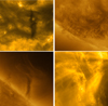 |
Fig. 19. Examples of filaments and prominences observed in HRIEUV in 2022 March (see Sect. 3.2.4). |
| In the text | |
|
Fig. 20. Mosaic of prominence eruptions observed by FSI in the 30.4 nm passband in 2022 March. The “enhance off-limb” functionality of JHelioviewer (Müller et al. 2017) was used when creating these graphics (see Sects. 3.3 and 3.3.3). |
| In the text | |
|
Fig. 21. FSI observations in the 17.4 nm passband of the C2.8 flare on 2022 March 10 (see Sect. 3.3.1). The images present the arcades of the post-flare loops. |
| In the text | |
|
Fig. 22. Time sequence of the eruption on 2022 March 21, as seen by FSI in the 30.4 nm passband. The “enhance off-limb” functionality of JHelioviewer (Müller et al. 2017) was used when creating these graphics (see Sect. 3.3.2). |
| In the text | |
|
Fig. 23. Enlargements of selected compact features observed by FSI at 17.4 nm on 2022 March 7 at 06:20:30 UT. Assuming that the sources are unresolved, the green and red profiles (horizontal and vertical, respectively) indicate a FWHM width of the effective PSF of 1.5 pixels (see Sect. 4.3). |
| In the text | |
|
Fig. 24. Enlargements of selected compact features observed by HRIEUV on 2022 March 7 at 00:41:55 UT. Assuming that the sources are unresolved, the green and red profiles (horizontal and vertical, respectively) indicate a FWHM width of the effective PSF of 1.5 pixels (see Sect. 4.3). |
| In the text | |
|
Fig. 25. HRILya observations of a set of quiet-Sun regions located near disk center, obtained on 2022 March 8 (panel a), 2022 March 22 (panel b), and 2022 March 30 (panel c; see Sect. 4.3). |
| In the text | |
Current usage metrics show cumulative count of Article Views (full-text article views including HTML views, PDF and ePub downloads, according to the available data) and Abstracts Views on Vision4Press platform.
Data correspond to usage on the plateform after 2015. The current usage metrics is available 48-96 hours after online publication and is updated daily on week days.
Initial download of the metrics may take a while.