| Issue |
A&A
Volume 699, July 2025
|
|
|---|---|---|
| Article Number | A138 | |
| Number of page(s) | 11 | |
| Section | The Sun and the Heliosphere | |
| DOI | https://doi.org/10.1051/0004-6361/202554650 | |
| Published online | 03 July 2025 | |
Extreme-ultraviolet transient brightenings in the quiet-Sun corona
Closest perihelion observations with Solar Orbiter/EUI
1
Solar-Terrestrial Centre of Excellence – SIDC, Royal Observatory of Belgium, Ringlaan -3- Av. Circulaire, 1180 Brussels, Belgium
2
Université Paris-Saclay, CNRS, Institut d’Astrophysique Spatiale, 91405 Orsay, France
3
Centre Spatial de Liège, Université de Liège, Av. du Pré-Aily B29, 4031 Angleur, Belgium
4
Max-Planck-Institut für Sonnensystemforschung, Justus-von-Liebig-Weg 3, 37077 Göttingen, Germany
5
Mathematics Institute, St Andrews University, KY16 9SS St Andrews, UK
6
Centre for mathematical Plasma Astrophysics (CmPA), Department of Mathematics, KU Leuven, 3001 Leuven, Belgium
7
Institute of Geodynamics of the Romanian Academy, Bucharest, Romania
⋆ Corresponding author: This email address is being protected from spambots. You need JavaScript enabled to view it.
Received:
19
March
2025
Accepted:
6
May
2025
Abstract
Context. The extreme-ultraviolet (EUV) brightenings identified by Solar Orbiter, commonly known as campfires, are the smallest transient brightenings detected to date outside active regions in the solar corona.
Aims. In order to understand their possible contribution to quiet-Sun heating, we investigated the spatio-temporal distribution of a large ensemble of the finest scale EUV transient brightenings observed by the Extreme Ultraviolet Imager (EUI) aboard Solar Orbiter.
Methods. We performed a statistical analysis of the EUV brightenings by using quiet-Sun observations at the highest possible spatial resolution ever obtained by the EUI. We used observations in the 17.4 nm passband of the High Resolution EUV Imager (HRIEUV) of EUI acquired during the closest perihelia of Solar Orbiter in 2022 and 2023. Solar Orbiter being at a distance 0.293 AU from the Sun, these observations have an exceptionally high image scale of 105 km, recorded at a fast cadence of 3 seconds. We used a wavelet-based automatic detection algorithm to detect and characterise the events of interest, and we studied their morphological and photometrical properties.
Results. We report the detection of the smallest and shortest lived EUV brightenings to date in the quiet Sun. The size and lifetime of the detected EUV brightenings appear power-law distributed down to a size of 0.01 Mm2 and a lifetime of 3 seconds. In general, their sizes lie in the range of 0.01 Mm2 to 50 Mm2, and their lifetimes vary between 3 seconds and 40 minutes. We find an increasingly high number of EUV brightenings on smaller spatial and temporal scales. We estimate that about 3600 EUV brightenings appear per second on the whole Sun. The HRIEUV brightenings thus represent the most prevalent, localised, and finest scale transient EUV brightenings in the quiet regions of the solar corona.
Conclusions. Using observations from EUI/HRIEUV at the highest possible achievable spatial resolution with the fastest cadence ever attained for quiet-Sun EUV observations, we detect the smallest and shortest lived EUV brightenings to date. Future studies that can provide estimates of the thermal energy content of the smallest-scale EUV brightenings will help to provide better insights into their role in the coronal heating.
Key words: magnetic reconnection / instrumentation: high angular resolution / Sun: corona / Sun: transition region / Sun: UV radiation
© The Authors 2025
 Open Access article, published by EDP Sciences, under the terms of the Creative Commons Attribution License (https://creativecommons.org/licenses/by/4.0), which permits unrestricted use, distribution, and reproduction in any medium, provided the original work is properly cited.
This article is published in open access under the Subscribe to Open model. This email address is being protected from spambots. You need JavaScript enabled to view it. to support open access publication.
1. Introduction
The ubiquitous presence of localised transient brightenings throughout the solar atmosphere is generally attributed to an impulsive release of energy by the process of magnetic reconnection (Klimchuk 2015; Pontin & Priest 2022). The nanoflare heating model of the quiet solar corona was proposed in Parker (1988) and further developed in Priest et al. (2002). The tectonics model in Priest et al. (2002) involves the prevalence of small-scale transient events or bursts, driven by magnetic reconnection (Parker 1972, 1983a,b) due to misaligned magnetic field strands, occurring continuously at small spatial and temporal scales in the solar atmosphere. This misalignment and structuring of the events in the corona are likely caused by the rapidly evolving small-scale magnetic elements on the solar surface. For instance, Smitha et al. (2017) discovered an order of magnitude more photospheric flux cancellation events than previously known at the boundaries of many granules, which has led to the development of a flux-cancellation model (Priest et al. 2018) for heating the chromosphere and corona and even accelerating the solar wind (Pontin et al. 2024).
In the solar transition region and lower corona, a plethora of small-scale localised brightening events in the quiet Sun, with typical length scales of a few Megameters, has been documented in the literature (Harrison et al. 2003; Young et al. 2018). Transition region explosive events (TREEs) are the most widely studied in this category (Brueckner & Bartoe 1983; Dere et al. 1989; Dere 1994; Innes et al. 1997; Teriaca et al. 2002, 2004). TREEs are generally characterised by their broad and multi-component spectral profiles in typical transition-region emission lines. Other classes of localised brightenings in the quiet Sun detected from various EUV imaging instruments include, but are not limited to, Blinkers (Harrison 1997), EUV transients (Berghmans et al. 1998), and many other micro-to-nano-flare-type transient events (Krucker & Benz 1998; Aschwanden et al. 2000a,b; Parnell & Jupp 2000; Benz & Krucker 2002; Joulin et al. 2016; Chitta et al. 2021; Purkhart & Veronig 2022; Belov et al. 2024). Despite the detections of a variety of EUV transients in the micro-to-nano-flare energy range, their estimated energy-flux rates have been reported to be insufficient to balance the coronal quiet-Sun energy losses (Withbroe & Noyes 1977; Aschwanden et al. 2016). Given the power-law-like distribution of the sizes and lifetimes of transient events in the corona, the determination of these characteristics on finer scales has remained a reflection of the limitations of the instruments; this is in terms of spatial and temporal resolutions, rather than an actual characterisation of the events.
Recently, Berghmans et al. (2021) reported the smallest EUV transient brightenings or bursts in the solar corona to date, which were identified by the High-Resolution EUV Imager (HRIEUV) of the Extreme Utraviolet Imager (EUI, Rochus et al. 2020) on board the Solar Orbiter (Müller et al. 2020). Commonly known as campfires, these EUV brightenings appear in the lower corona and above the locations of supergranular network boundaries. They have been reported to have sizes between 0.08 Mm2 and 5 Mm2 and durations between 10 s and 200 s by Berghmans et al. (2021). Combining the observations of HRIEUV and Atmospheric Imaging Assembly (AIA, Lemen et al. 2012) on board the Solar Dynamics Observatory (SDO, Pesnell et al. 2012), and using stereoscopic techniques, Zhukov et al. (2021) found that these EUV brightenings are typically formed over the transition region to the lower corona, i.e. at heights between 1 Mm and 5 Mm in the solar atmosphere.
Recent magnetohydrodynamic simulations (Chen et al. 2021, 2025) and magnetic-field extrapolations (Barczynski et al. 2022) have indicated that magnetic reconnection in the transition region and lower corona is the likely mechanism behind the generation of EUV brightenings observed by HRIEUV. By studying the photospheric magnetic field at the base of the EUV brightenings, Panesar et al. (2021) and Kahil et al. (2022) showed that many of the EUV brightenings observed by HRIEUV occur above the locations of small-scale bipolar magnetic elements, which is consistent with the flux-cancellation model (Priest et al. 2018; Pontin et al. 2024). Furthermore, Nelson et al. (2024) found that these EUV brightenings preferentially appear co-spatial with the strong (> 20 G) photospheric network field, though they predominantly do not occur co-spatial with bipolar magnetic elements.
Using EUV observations from the AIA, Chitta et al. (2021) also reported the presence of EUV transient brightenings or EUV bursts in the quiet Sun. These EUV bursts were reported to have sizes in the range of 0.2 Mm2 to 10 Mm2 and lifetimes between 36 s and 400 s in Chitta et al. (2021). The occurrence rate of these EUV bursts was found to be a factor of 100 lower than that required to balance the quiet-Sun energy requirement. The EUV brightenings reported in Berghmans et al. (2021) have an occurrence rate that is almost twice that of the EUV bursts reported in Chitta et al. (2021). The higher spatial and temporal resolution of HRIEUV, and its higher radiometric sensitivity (Gissot et al. 2023; Shestov et al. 2025) in comparison to AIA can be considered as an important reason for the higher number of detections in the former case. The HRIEUV observations in Berghmans et al. (2021) have a one-pixel resolution of 200 km and a cadence of 5 s, while the AIA observations in Chitta et al. (2021) have those of 435 km and 12 s. Even with the high-resolution observations of HRIEUV, the number of EUV brightenings reported in Berghmans et al. (2021) still represents a deficit of at least 50 times the required rate to account for the quiet-Sun coronal-energy requirements. This deficit can be improved by using much better spatially and temporally resolved observations to aid the detections of yet unresolved structures in the solar corona.
At the same time, there is also an active debate on the thermal properties of EUV brightenings observed by EUI along with their overall contribution to the coronal heating requirements. Based on imaging observations of EUI with AIA, Berghmans et al. (2021) found that the EUV brightenings reach temperatures of 1 MK, while Dolliou et al. (2023) indicated that this may not be the case for all EUV brightenings. Additionally, by studying a sample of EUV brightenings with UV/EUV spectroscopic observations, Huang et al. (2023) and Dolliou et al. (2024) showed that many of the EUV brightenings may have temperatures below 1 MK.
As is the case for all observations, the smallest size and shortest lifetime reported for the EUV brightenings observed by HRIEUV and the EUV bursts observed by AIA are also limited by the spatial and temporal resolution of the respective observations employed. Here, we present the HRIEUV observations taken during the closest perihelion of Solar Orbiter at about 0.293 AU from the Sun. At the closest proximity to the Sun that Solar Orbiter can achieve, these unique observations possess the highest possible spatial resolution that can be achieved by HRIEUV. These observations have spatial and temporal resolutions about two times better than those used in Berghmans et al. (2021) and the other EUV brightenings related studies using HRIEUV mentioned above, and four times better than the AIA observations used in Chitta et al. (2021). The HRIEUV passband centred at the 17.4 nm has a peak temperature response close to 1 MK. We took advantage of the unique EUV observations of the quiet-Sun corona with unprecedented resolution provided by HRIEUV in close proximity to the Sun to perform a statistical study of the properties of smallest-scale EUV brightenings which were previously inaccessible. As these brightenings are imprints of fine-scale magnetic reconnection, we explored their possible role in heating quiet regions of the solar corona. We use the term EUV brightenings for the transient small-scale EUV brightenings or EUV bursts observed by HRIEUV up to its resolution limit.
2. Solar Orbiter/EUI perihelion observations
Solar Orbiter has a unique orbit (Müller et al. 2020; Zouganelis et al. 2020), and, by virtue of this, it can achieve the closest proximity to the Sun (Solar Orbiter perihelion); that is, just 0.293 AU away from the Sun. Berghmans et al. (2023) showcased the details of EUI observations for the Solar Orbiter’s first close perihelion. In this study, we used the quiet-Sun observations at the Solar Orbiter perihelion (0.293 AU) of HRIEUV in the 17.4 nm passband taken on 12 October 2022 from 05:25:00 UTC to 06:09:30 UTC (dataset-1) and on 6 October 2023 from 10:00:00 UTC to 11:00:00 UTC (dataset-2). Both the datasets were obtained as part of the Solar Orbiter Observing Plan named R_SMALL_HRES_HCAD_RS-burst (Zouganelis et al. 2020). The HRIEUV images have a pixel scale of 0.492″ (Gissot et al. 2023), which for these observations correspond to approximately 105 km on the solar surface. These observations have the highest possible spatial resolution that can be achieved by HRIEUV. They have an extremely high cadence of 3 s, which is the best suitable fast cadence with which HRIEUV can obtain good-quality quiet-Sun observations. These unique HRIEUV datasets thus constitute the best resolved, spatially and temporally, observations of the quiet Sun ever obtained in EUV passbands. The observations used here are the best of their kind to date to study the EUV brightenings occurring on the finest spatial and temporal scales.
We used the level-2 calibrated release-6 data of EUI/HRIEUV (Kraaikamp et al. 2023) available on the EUI website1 and in the Solar Orbiter Data Archive (SOAR2). The release-6 data of EUI has considerable improvements in terms of pointing information and provides significantly stable data sequences. The images from dataset-1 were also employed by Chitta et al. (2023) to study properties of quiet-Sun coronal loops and their relation to the underlying surface-magnetic-field distribution. The duration of dataset-1 is almost 45 minutes, and that of dataset-2 is 60 minutes. The exposure time for all the images in the two datasets studied here is 1.65 seconds. With a pixel scale of 105 km, the field of view (FoV) of 2048 × 2048 HRIEUV pixels corresponds to 215 Mm × 215 Mm on the surface of the Sun for both of the datasets. An example of the HRIEUV FoV of the two datasets is shown in Fig. 1 with context images of the full disc of the Sun as captured by the Full Sun Imager (FSI; aboard EUI). During both sets of observations, the Solar Orbiter’s orbit was at an inclination of about 4° towards the solar south with respect to Earth’s orbital plane. The separation angle of the Solar Orbiter with respect to the Sun-Earth line was approximately 120° during these observations, and thus no coordinated observations were possible in these cases with the Earth-aligned observatories.
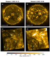 |
Fig. 1. Representative images of both EUI quiet-Sun observations studied in this article. Panels a and b show the visualisation from JHelioviewer (Müller et al. 2017), where the EUI/FSI 17.4 nm images overlaid with the near-simultaneous HRIEUV images are shown. The time mentioned in UTC corresponds to the time of observation at the Solar Orbiter. Carrington coordinates are shown, the crossing of the two yellow great circles indicates the antipode of the Earth/SDO sub-solar point. The red and blue markers indicate the solar north and south poles. Panels c and d show the HRIEUV images that cover a FoV of approximately 20° in longitude and latitude, corresponding to 215 Mm × 215 Mm on the surface of the Sun for both datasets. The detected EUV brightenings at the specific instance are marked in cyan over the respective FoVs for illustrative purposes. Movie 1 and movie 2 (available online) show the detected EUV brightenings over the full FoV for the complete duration of the two data-sequences. |
Note that some portion at the top right corner of the HRIEUV FoV of dataset-2 is covered by coronal loops that belong to a non-flaring active region present in the vicinity of the FoV (see Figs. 1b and d). As these active-region coronal loops cover only a small portion of the FoV and are stable throughout the data-sequence, we consider that dataset-2 mostly contains quiet-Sun environment. Each of the two quiet-Sun datasets used here cover almost 0.75% of the solar surface and contain the observation sequences for long durations of almost 45−60 minutes. The quiet-Sun region spanned by these observations can thus be considered as typical quiet coronal environment present over the solar surface at any given instance. Subsequently, the properties of EUV brightenings studied here should be treated as such for the average population of EUV brightenings present in quiet regions of the Sun.
3. Analysis and results
3.1. Detection of EUV brightenings
We detected EUV brightenings in both datasets by using the algorithm employed in Berghmans et al. (2021). This wavelet-based automated detection scheme separates the small space-time transient events from random intensity fluctuations by determining their statistical significance against the noise present in the data. The relevant details about the detection scheme are provided in Appendix A. The detection algorithm reveals the EUV brightenings with their ubiquitous presence across the FoV. We detect a total of 79089 EUV brightenings in dataset-1 and 98649 EUV brightenings in dataset-2. Figures 1c and d show the detected EUV brightenings at a particular instance over the FoV of the two datasets. We observe that there is tendency for the EUV brightenings to appear in groups (see movie 1 and movie 2, available online). Figure 2 shows six illustrative examples of a close-up view of the EUV brightenings, with additional examples provided in Appendix B. The smallest EUV brightenings detected have an area of 0.01 Mm2, and the shortest lived ones have a lifetime of 3 s. These minimum values of the detected size and lifetime of EUV brightenings represent the image scale and cadence limit of the observations. Note that the above-quoted values do not include the individual events of one spatial-pixel which exist only in a single time-frame. However, the one spatial-pixel events that last for several time-frames and one time-frame events that consist of several spatial-pixels are considered in the analysis. Such events, respectively, constitute 2% and 51% of the total number of EUV brightenings studied here. Thus, we are limited more by the temporal cadence than the spatial resolution of the observations in detecting the small-scale events that evolve on much shorter timescales.
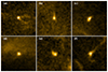 |
Fig. 2. Illustrative examples of close-up view of six EUV brightenings. The FoV of each panel is 4 Mm × 4 Mm. |
3.2. Spatial distribution of EUV brightenings
The average value of the number of EUV brightenings present in every frame of dataset-1 is found to be about 390, and that of dataset-2 is about 350. Their spatial area coverage over the respective FoV is estimated to have an average value of 0.11% for dataset-1 and 0.08% for dataset-2. Despite their ubiquitous and pervasive nature, EUV brightenings are observed to avoid the core of the medium-to-large-scale coronal loops present in the FoV. In the close neighbourhood of such structures, the EUV brightenings are preferably present near their foot points. As mentioned above, the number of EUV brightenings per frame and their spatial area coverage in dataset-2 is slightly less than in dataset-1. This is due to the presence of loop structures in the dataset-2 that cover some portion of the top right corner of the FoV (see Figs. 1b and d). These coronal loops, as mentioned in Sect. 2, are part of the active region present in the vicinity of the observed FoV.
With the total number of EUV brightenings detected in each dataset and dividing it by the spatial area of the FoV and duration of respective dataset, we find the occurrence rate of the EUV brightenings from dataset-1 to be 6.3 × 10⁻¹⁶ m−2 s−1 and that from dataset-2 to be 5.9 × 10⁻¹⁶ m−2 s−1. This gives an estimated average occurrence rate of EUV brightenings over the whole surface area of the Sun of approximately 3600 per second. These values are more than one order of magnitude higher than the EUV brightenings reported in Berghmans et al. (2021) and Nelson et al. (2024) and the EUV bursts reported in Chitta et al. (2021). Note that Berghmans et al. (2021) and Nelson et al. (2024) used the same detection algorithm as in this sudy, while the detection scheme used in Chitta et al. (2021) was compeletly different. The increase in the number of detected EUV transient brightenings is thus primarily due to the extremely high resolution of HRIEUV at the Solar Orbiter perihelion in comparison to other observations (as described in Sects. 1 and 2). However, if the two datasets studied here represent unusual quiet-Sun regions that display an excess of enhanced small-scale transient activity in form of EUV brightenings, the ubiquitous and pervasive presence of EUV brightenings may not be the average nature of a common quiet-Sun region. In such a case, the high occurence rate of EUV brightenings detected here could be the combined effect of higher resolution and an enhanced small-scale activity of these exceptional quiet-Sun regions. Neverthless, the EUV brightenings detected and studied here are the most prevalent, localised, and smallest scale quiet-Sun EUV transient brightenings detected in the solar corona to date.
3.3. Morphological and photometrical properties
We estimated the morphological properties (surface area, lifetime, volume, and aspect ratio) and photometrical properties (total brightness, average brightness, and peak brightness) of all the EUV brightenings detected in both the datasets. Appendix A provides the definition for the above-mentioned properties of the EUV brightenings. Figure 3 shows, for both datasets, the distribution of the average brightness of the EUV brightenings in comparison to the pixel brightness values of the temporally averaged FoV. The distributions of the average brightness of EUV brightenings fall along the higher values of the respective distributions for the pixel brightness of the average FoV. As quoted in Fig. 3, the mean values of the distribution for the average brightness of the EUV brightenings are about 1.6 to 2.0 times larger than the mean values of the distributions for the pixel brightness values of the average FoV. The temporally averaged FoV can be considered to represent the local background conditions. This indicates that the average member of the population of EUV brightenings detected in our observations has an approximately 50% brightness enhancement compared to the background quiet-Sun emission.
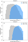 |
Fig. 3. Distributions of average brightness of EUV brightenings detected in the two datasets are shown in blue in each panel. Over-plotted are the respective distributions of pixel brightness of the temporally averaged FoV in grey. The overlapping region of the two distributions is shown in dark blue. The axes of both plots are shown with a log10 scale. |
The distribution of properties of EUV brightenings are studied further with the help of histograms and scatter plots that are shown in Figs. 4 and 5 for dataset-1, and in Figs. C.1 and C.2 for dataset-2 (Appendix C), respectively. Noticeably, the respective distributions for the two datasets show very similar trends. The detected EUV brightenings have surface areas in the range of 0.01 Mm2 to 50 Mm2 and lifetimes from 3 seconds to 40 minutes. The distribution of the properties of EUV brightenings in Fig. 4 shows that, within the detected population of EUV brightenings, their surface area and lifetime vary by almost three orders of magnitude. We performed a maximum-likelihood power-law fit (Clauset et al. 2009; Alstott et al. 2014) to the probability density functions estimated from the histograms of surface area, lifetime, volume, and total brightness. The calculated power-law indices are quoted in the respective panels of Fig. 4 for dataset-1, and similarly in Fig. C.1 of Appendix C for dataset-2. The obtained values of power-law indices for the distribution of size and lifetime are similar to those mentioned in Berghmans et al. (1998) for quiet-Sun EUV transient brightenings observed by the Extreme-ultraviolet Imaging Telescope (EIT, Delaboudinière et al. 1995) aboard the Solar and Heliospheric Observatory. This indicates that the small-scale EUV brightenings detected by different resolution instruments may follow the similar scaling laws and are possibly part of the same nanoflare family. The aspect-ratio histogram in Fig. 4 reveals that the events with an almost symmetric shape (aspect ratio < 3.0) are more numerous than those with an asymmetric shape (aspect ratio > 3.0). With the power-law behaviour of the distribution of the surface area, lifetime, and volume; the smaller, short-lived and events with symmetric morphology dominate in the detected population of EUV brightenings.
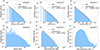 |
Fig. 4. Probability density distributions of properties of EUV brightenings for dataset-1. The probability density function (PDF) and power-law fit are shown for the distributions of surface area, lifetime, volume, and total intensity. The axes of all the plots are shown with a log10 scale. The corresponding figure for dataset-2 is shown in Appendix C. |
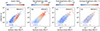 |
Fig. 5. Relations between different properties of EUV brightenings for dataset-1. The scatter plot between surface area and lifetime is shown along with trends related to other morphological and photometrical properties in different panels. The axes of all the plots are shown with a log10 scale. The corresponding figure for dataset-2 is shown in Appendix C. |
The scatter plots in Fig. 5 for dataset-1 show the interrelation between different properties of EUV brightenings. The different panels in Fig. 5 show the scatter plot between surface area and lifetime and their association with aspect ratio in panel a, total brightness in panel b, peak brightness in panel c and average brightness panel d. The corresponding scatter plots for dataset-2 are shown in Fig. C.2 of Appendix C. The value of Spearman’s correlation coefficient between surface area and lifetime is found to be 0.71 for both datasets. The scatter plot shown in Fig. 5a hints that populations of the EUV brightenings show distinct behaviour with respect to aspect ratio depending on whether their surface area is larger or smaller than 0.2 Mm2. Among the EUV brightenings detected in each dataset, almost 93% of the events have a surface area under 0.2 Mm2. The lifetimes of the EUV brightenings in the population with a surface area smaller than 0.2 Mm2 lie between 3 s and 2 min. Among this population group, 91% of EUV brightenings are of almost symmetric shape with an aspect ratio less than 3.0. While among the population group with a surface area larger than 0.2 Mm2, 55% of the EUV brightenings are of asymmetric shape with an aspect ratio over 3.0. Among these two population groups, there is no distinction observed in terms of their spatial distribution across the FoV. This illustrates that, though randomly spread across the FoV, the smaller and short-lived EUV brightenings are dominated by almost circular events, and larger and longer-lived events are mostly elongated in shape.
The scatter plots shown in Figs. 5b–d show that the morphological properties of EUV brightenings have positive association with their photometrical properties. As shown in Fig. 5b there is a strong positive association of total brightness with respect to the variation of surface area and lifetime. This is primarily due to the intrinsic definition of total brightness of the event, that is the integrated brightness of the event over its area and duration. Such a positive association of surface area and lifetime is also present for the case of peak brightness (Fig. 5c), though the trend is not as strong as that for the case of total brightness. For the case of average brightness (Fig. 5d) the trend is comparatively weaker. Such associations between surface area, lifetime, aspect ratio, and brightness of the EUV brightenings show that there is a tendency for spatially smaller, symmetrical, and shorter lived EUV brightenings to have lower values of brightness, and for larger, asymmetrical, and longer lived EUV brightenings to have higher values of brightness. The statistical distribution and interrelation among different properties of EUV brightenings presented in this section show that the population group of small events (0.01 Mm2 < surface area < 0.2 Mm2), which are mostly short lived (3 s < lifetime < 2 min), almost circular, and not very bright in comparison to others, represent the dominant group within the detected population of EUV brightenings. Such a population of fine-scale EUV brightenings has become accessible by the virtue of high spatial and temporal resolution of HRIEUV with its high radiometric sensitivity.
4. Discussion
Previous studies of small-scale coronal transients indicate that nanoflare heating might not be sufficient to account for the coronal energy losses outside the active regions of the Sun (Aschwanden et al. 2000b; Benz & Krucker 2002; Joulin et al. 2016; Chitta et al. 2021; Purkhart & Veronig 2022), primarily due to the low occurrence rate of such low-energy events in the quiet Sun. With the high spatial and temporal resolution observations of HRIEUV presented in this study, an increasingly high occurrence rate of the EUV brightenings is observed at finer spatial and temporal scales. If these events reach coronal temperatures of 1 MK or more, they can be possible candidates for quiet-Sun coronal heating. On the other hand, the high occurrence rate and the ubiquitous and pervasive nature of EUV brightenings observed in the two datasets studied here may not represent the average behaviour of quiet-Sun corona in general. For instance, Gorman et al. (2023) showed specific cases of large sections of the quiet-Sun corona, on supergranular scales, that lack clear signatures of transient EUV-brightening-type events, giving rise to the coronal appearance that is very diffuse.
Berghmans et al. (2021) derived temperatures of about 1 MK for most of the EUV brightenings observed by HRIEUV, and their physical heights have been found to be limited up to lower corona (Zhukov et al. 2021). By studying a sample of EUV brightenings, Huang et al. (2023) and Dolliou et al. (2023, 2024) indicated that many of these events may have temperatures below 1 MK and are chromospheric or transition-region events. Nelson et al. (2023) also showed that many of the EUV brightenings display a discernible transition-region response. However, due to the limited resolution of the supplementary imaging and spectral observations used with HRIEUV in the above-mentioned studies, significant conclusions cannot be made about the smallest scale EUV brightenings observed by HRIEUV. While it is important to note that by using a 3D self-consistent quiet-Sun model of resolution comparable to HRIEUV, Chen et al. (2025) indicate that the EUV brightenings observed by HRIEUV may be composed of a mix of different populations of events, with some of the events reaching coronal temperatures of 1 MK and above, while others remain at transition-region temperatures.
Estimating the temperature and thermal energy flux for the EUV brightenings is crucial to addressing their role in coronal heating. The HRIEUV passband centred at 17.4 nm has an effective width of 0.5 nm (Gissot et al. 2023). With the peak temperature response of the HRIEUV passband close to 1 MK, the HRIEUV observations have contributions from solar plasma with temperatures in the range of 0.3 MK to 1.2 MK (Shestov et al. 2025). Thus, multi-wavelength imaging and spectral observations with high spatial, temporal, and wavelength resolutions are crucial for a better understanding of the temperature and density of the smallest scale HRIEUV brightenings. The joint observations of EUI/HRIEUV with upcoming missions in near future, such as EUV High-Throughput Spectroscopic Telescope (EUVST, Shimizu et al. 2019) aboard Solar–C and Multi-slit Solar Explorer (MUSE, De Pontieu et al. 2022), will be of utmost importance in this context.
5. Conclusions
In this article, we present the highest resolution observations of the quiet solar corona available to date. The HRIEUV telescope of EUI on board the Solar Orbiter obtained such observations during its perihelia. Using two such sets of observations we have detected the smallest, shortest lived, and most prevalent EUV transient brightenings reported till now, with sizes down to 0.01 Mm2 and lifetimes of 3 s. We find that the EUV brightenings are ubiquitous, with 79089 EUV brightenings present in dataset-1 and 98649 in dataset-2. Their spatial area coverage is about 0.1% with a high occurrence rate of about 6.1 × 10⁻¹⁶ m−2 s−1 over quiet regions of the Sun. This gives an average occurrence rate over the whole surface area of the Sun of approximately 3600 EUV brightenings per second. This occurrence rate is more than one order of magnitude greater than that for the previously reported values for the similar events (Chitta et al. 2021; Berghmans et al. 2021; Nelson et al. 2024). This is primarily by virtue of high spatial and temporal resolution observations of HRIEUV obtained at the closest perihelia of the Solar Orbiter. Given that the observations used in this study have the best possible spatial resolution achievable by HRIEUV, higher cadence observations of the quiet Sun – while maintaining the highest possible spatial resolution – may reveal an even higher occurrence rate of EUV brightenings. Such EUI/HRIEUV observations are planned for the Solar Orbiter’s perihelion in the near future. However, great caution must be exercised regarding the exposure time of faster cadence observations to maintain sufficient signal levels, particularly when observing the quiet, low-emission regions of the solar corona.
We studied the statistical distribution and interrelation among different morphological and photometrical properties of EUV brightenings. We find power-law behaviour in the distribution of the surface area and lifetime of the EUV brightenings. A positive correlation is seen between these properties of the brightenings. We find that among the detected EUV brightenings spatially smaller and shorter-lived events predominantly have an almost symmetric shape and circular mophology. On the other hand, the larger and longer duration events mostly have asymmetric shapes and elongated morphology. A positive association is observed between the brightness of the EUV brightenings and their surface areas and lifetimes. We find a general trend of smaller and shorter lived events having lower values of brightness, and larger and longer lived ones have higher values of brightness.
We find that EUV brightenings with a surface area smaller than 0.2 Mm2 and lifetimes shorter than 2 min represent the dominant population group within the detected EUV brightenings. Thus, the high spatial and temporal resolution of HRIEUV with its high radiometric sensitivity is indispensable to study the smallest scale EUV brightenings in details. However, our understanding of the thermal properties of the HRIEUV transient brightenings remains elusive due to the current absence of high-resolution multi-wavelength imaging and spectral observations. Such high-resolution observations coordinated with HRIEUV that can simultaneously map transition region and corona are necessary in this context. Future solar missions such as MUSE and Solar–C/EUVST, in combination with Solar Orbiter/EUI observations, will provide unique opportunities to gain better insights into the finest scale events in the solar corona.
Data availability
Movies associated to Fig. 1 are available at https://www.aanda.org
Acknowledgments
Authors thank anonymous referee for constructive comments. Solar Orbiter is a space mission of international collaboration between ESA and NASA, operated by ESA. The EUI instrument was built by CSL, IAS, MPS, MSSL/UCL, PMOD/WRC, ROB, LCF/IO with funding from the Belgian Federal Science Policy Office (BELSPO/PRODEX PEA 4000106864, 4000112292 and 4000134088); the Centre National d’Etudes Spatiales (CNES); the UK Space Agency (UKSA); the Bundesministerium für Wirtschaft und Energie (BMWi) through the Deutsches Zentrum für Luftund Raumfahrt (DLR); and the Swiss Space Office (SSO). N.N. acknowledges funding from the Belgian Federal Science Policy Office (BELSPO) contract B2/223/P1/CLOSE-UP. C.V. and L.D. thanks BELSPO for the provision of financial support in the framework of the PRODEX Programme of the European Space Agency (ESA) under contract numbers 4000143743, 4000134088 and 4000136424. L.P.C. gratefully acknowledges funding by the European Union (ERC, ORIGIN, 101039844). Views and opinions expressed are however those of the author(s) only and do not necessarily reflect those of the European Union or the European Research Council. Neither the European Union nor the granting authority can be held responsible for them. This research was supported by the International Space Science Institute (ISSI) in Bern, through ISSI International Team project #23-586 (Novel Insights Into Bursts, Bombs, and Brightenings in the Solar Atmosphere from Solar Orbiter). Authors thank Dr. Susanna Parenti and Prof. Louise Harra for helpful discussions. JHelioviewer software was used in this research to visualise EUI observations. SSWIDL and various Python packages including sunpy and astropy were used for the data analysis. This work has used NASA’s Astrophysics Data System.
References
- Alstott, J., Bullmore, E., & Plenz, D. 2014, PLoS One, 9, 1 [Google Scholar]
- Aschwanden, M. J., Nightingale, R. W., Tarbell, T. D., & Wolfson, C. J. 2000a, ApJ, 535, 1027 [Google Scholar]
- Aschwanden, M. J., Tarbell, T. D., Nightingale, R. W., et al. 2000b, ApJ, 535, 1047 [Google Scholar]
- Aschwanden, M. J., Crosby, N. B., Dimitropoulou, M., et al. 2016, Space Sci. Rev., 198, 47 [Google Scholar]
- Barczynski, K., Meyer, K. A., Harra, L. K., et al. 2022, Sol. Phys., 297, 141 [NASA ADS] [CrossRef] [Google Scholar]
- Belov, S. A., Bogachev, S. A., Ledentsov, L. S., & Zavershinskii, D. I. 2024, A&A, 684, A60 [NASA ADS] [CrossRef] [EDP Sciences] [Google Scholar]
- Benz, A. O., & Krucker, S. 2002, ApJ, 568, 413 [Google Scholar]
- Berghmans, D., Clette, F., & Moses, D. 1998, A&A, 336, 1039 [NASA ADS] [Google Scholar]
- Berghmans, D., Auchère, F., Long, D. M., et al. 2021, A&A, 656, L4 [NASA ADS] [CrossRef] [EDP Sciences] [Google Scholar]
- Berghmans, D., Antolin, P., Auchère, F., et al. 2023, A&A, 675, A110 [NASA ADS] [CrossRef] [EDP Sciences] [Google Scholar]
- Brueckner, G. E., & Bartoe, J. D. F. 1983, ApJ, 272, 329 [Google Scholar]
- Chen, Y., Przybylski, D., Peter, H., et al. 2021, A&A, 656, L7 [NASA ADS] [CrossRef] [EDP Sciences] [Google Scholar]
- Chen, Y., Peter, H., & Przybylski, D. 2025, A&A, 693, A29 [NASA ADS] [CrossRef] [EDP Sciences] [Google Scholar]
- Chitta, L. P., Peter, H., & Young, P. R. 2021, A&A, 647, A159 [NASA ADS] [CrossRef] [EDP Sciences] [Google Scholar]
- Chitta, L. P., Solanki, S. K., del Toro Iniesta, J. C., et al. 2023, ApJ, 956, L1 [NASA ADS] [CrossRef] [Google Scholar]
- Clauset, A., Shalizi, C. R., & Newman, M. E. J. 2009, SIAM Rev., 51, 661 [NASA ADS] [CrossRef] [Google Scholar]
- De Pontieu, B., Testa, P., Martínez-Sykora, J., et al. 2022, ApJ, 926, 52 [NASA ADS] [CrossRef] [Google Scholar]
- Delaboudinière, J. P., Artzner, G. E., Brunaud, J., et al. 1995, Sol. Phys., 162, 291 [Google Scholar]
- Dere, K. P. 1994, Adv. Space Res., 14, 13 [Google Scholar]
- Dere, K. P., Bartoe, J. D. F., & Brueckner, G. E. 1989, Sol. Phys., 123, 41 [Google Scholar]
- Dolliou, A., Parenti, S., Auchère, F., et al. 2023, A&A, 671, A64 [NASA ADS] [CrossRef] [EDP Sciences] [Google Scholar]
- Dolliou, A., Parenti, S., & Bocchialini, K. 2024, A&A, 688, A77 [NASA ADS] [CrossRef] [EDP Sciences] [Google Scholar]
- Gissot, S., Auchère, F., Berghmans, D., et al. 2023, ArXiv e-prints [arXiv:2307.14182] [Google Scholar]
- Gorman, J., Chitta, L. P., Peter, H., et al. 2023, A&A, 678, A188 [NASA ADS] [CrossRef] [EDP Sciences] [Google Scholar]
- Harrison, R. A. 1997, Sol. Phys., 175, 467 [Google Scholar]
- Harrison, R. A., Harra, L. K., Brković, A., & Parnell, C. E. 2003, A&A, 409, 755 [NASA ADS] [CrossRef] [EDP Sciences] [Google Scholar]
- Huang, Z., Teriaca, L., Aznar Cuadrado, R., et al. 2023, A&A, 673, A82 [NASA ADS] [CrossRef] [EDP Sciences] [Google Scholar]
- Innes, D. E., Inhester, B., Axford, W. I., & Wilhelm, K. 1997, Nature, 386, 811 [Google Scholar]
- Joulin, V., Buchlin, E., Solomon, J., & Guennou, C. 2016, A&A, 591, A148 [NASA ADS] [CrossRef] [EDP Sciences] [Google Scholar]
- Kahil, F., Hirzberger, J., Solanki, S. K., et al. 2022, A&A, 660, A143 [NASA ADS] [CrossRef] [EDP Sciences] [Google Scholar]
- Klimchuk, J. A. 2015, Phil. Trans. R. Soc. London Ser. A, 373, 20140256 [Google Scholar]
- Kraaikamp, E., Gissot, S., Stegen, K., et al. 2023, SolO/EUI Data Release 6.0 2023-01 (Royal Observatory of Belgium (ROB)), https://doi.org/10.24414/z818-4163 [Google Scholar]
- Krucker, S., & Benz, A. O. 1998, ApJ, 501, L213 [Google Scholar]
- Lemen, J. R., Title, A. M., Akin, D. J., et al. 2012, Sol. Phys., 275, 17 [Google Scholar]
- Lim, D., Van Doorsselaere, T., Berghmans, D., et al. 2025, A&A, 698, A65 [NASA ADS] [CrossRef] [EDP Sciences] [Google Scholar]
- Müller, D., Nicula, B., Felix, S., et al. 2017, A&A, 606, A10 [Google Scholar]
- Müller, D., St. Cyr, O. C., Zouganelis, I., et al. 2020, A&A, 642, A1 [Google Scholar]
- Murtagh, F., Starck, J. L., & Bijaoui, A. 1995, A&AS, 112, 179 [Google Scholar]
- Nelson, C. J., Auchère, F., Aznar Cuadrado, R., et al. 2023, A&A, 676, A64 [NASA ADS] [CrossRef] [EDP Sciences] [Google Scholar]
- Nelson, C. J., Hayes, L. A., Müller, D., et al. 2024, A&A, 692, A236 [NASA ADS] [CrossRef] [EDP Sciences] [Google Scholar]
- Panesar, N. K., Tiwari, S. K., Berghmans, D., et al. 2021, ApJ, 921, L20 [CrossRef] [Google Scholar]
- Parker, E. N. 1972, ApJ, 174, 499 [NASA ADS] [CrossRef] [Google Scholar]
- Parker, E. N. 1983a, ApJ, 264, 635 [Google Scholar]
- Parker, E. N. 1983b, ApJ, 264, 642 [Google Scholar]
- Parker, E. N. 1988, ApJ, 330, 474 [Google Scholar]
- Parnell, C. E., & Jupp, P. E. 2000, ApJ, 529, 554 [Google Scholar]
- Pesnell, W. D., Thompson, B. J., & Chamberlin, P. C. 2012, Sol. Phys., 275, 3 [Google Scholar]
- Pontin, D. I., & Priest, E. R. 2022, Liv. Rev. Sol. Phys., 19, 1 [NASA ADS] [CrossRef] [Google Scholar]
- Pontin, D. I., Priest, E. R., Chitta, L. P., & Titov, V. S. 2024, ApJ, 960, 51 [NASA ADS] [CrossRef] [Google Scholar]
- Priest, E. R., Heyvaerts, J. F., & Title, A. M. 2002, ApJ, 576, 533 [NASA ADS] [CrossRef] [Google Scholar]
- Priest, E. R., Chitta, L. P., & Syntelis, P. 2018, ApJ, 862, L24 [Google Scholar]
- Purkhart, S., & Veronig, A. M. 2022, A&A, 661, A149 [NASA ADS] [CrossRef] [EDP Sciences] [Google Scholar]
- Rochus, P., Auchère, F., Berghmans, D., et al. 2020, A&A, 642, A8 [NASA ADS] [CrossRef] [EDP Sciences] [Google Scholar]
- Shestov, S. V., Zhukov, A. N., Auchère, F., Berghmans, D., & Loicq, J. 2025, A&A, 699, A7 [NASA ADS] [CrossRef] [EDP Sciences] [Google Scholar]
- Shimizu, T., Imada, S., Kawate, T., et al. 2019, SPIE Conf. Ser., 11118, 1111807 [NASA ADS] [Google Scholar]
- Smitha, H. N., Anusha, L. S., Solanki, S. K., & Riethmüller, T. L. 2017, ApJS, 229, 17 [Google Scholar]
- Starck, J.-L., & Murtagh, F. 1994, A&A, 288, 342 [NASA ADS] [Google Scholar]
- Starck, J.-L., & Murtagh, F. 2002, Astronomical Image and Data Analysis (Berlin: Springer) [Google Scholar]
- Teriaca, L., Madjarska, M. S., & Doyle, J. G. 2002, A&A, 392, 309 [NASA ADS] [CrossRef] [EDP Sciences] [Google Scholar]
- Teriaca, L., Banerjee, D., Falchi, A., Doyle, J. G., & Madjarska, M. S. 2004, A&A, 427, 1065 [NASA ADS] [CrossRef] [EDP Sciences] [Google Scholar]
- Withbroe, G. L., & Noyes, R. W. 1977, ARA&A, 15, 363 [Google Scholar]
- Young, P. R., Tian, H., Peter, H., et al. 2018, Space Sci. Rev., 214, 120 [Google Scholar]
- Zhukov, A. N., Mierla, M., Auchère, F., et al. 2021, A&A, 656, A35 [NASA ADS] [CrossRef] [EDP Sciences] [Google Scholar]
- Zouganelis, I., De Groof, A., Walsh, A. P., et al. 2020, A&A, 642, A3 [NASA ADS] [CrossRef] [EDP Sciences] [Google Scholar]
Appendix A: Detection scheme for EUV brightenings
As mentioned in Sect. 3.1 we use the wavelet-based automated detection algorithm similar to that employed in Berghmans et al. (2021), to isolate the transient EUV brightenings occurring at small scales in the observations. We separate the small features of interest spatially by determining their statistical significance over the noise present in the data and track them in time through the observation sequence. The HRIEUV level-2 images are remapped to Carrington coordinates, with 105 km pitch, before subjecting them to the detection algorithm. The HRIEUV resolution is thus kept preserved while performing the coordinate transformation.
In the noise model we consider the photon shot noise and read-out noise which are the dominant sources of noise present in the HRIEUV observations (Rochus et al. 2020; Gissot et al. 2023). The small-scale transient brightenings of interest are detected using the first two scales of a dyadic ‘à trous’ wavelet transform of the images using a B3 spline scaling function (Starck & Murtagh 1994, 2002). Using the treatment of Murtagh et al. (1995) and applying Poisson statistics, wavelet coefficients in the first two scales are considered significant when they are greater than 6 times the root-mean-square amplitude expected from the noise model. Such a threshold puts a rigorous statistical significance criterion on the detection of the small-scale events with almost 99% confidence level against the dominant sources of noise present in the data. The thresholding of the wavelet coefficients in each image results in a binary cube. The 6-connected voxels in the space and time (x,y,t) dimensions of the binary cube are clustered into numbered regions. Each region defines an event i.e. an EUV brightening.
The above detection scheme is applied to both the datasets. The morphological properties (lifetime, surface area, volume and aspect ratio) and photometrical properties (total brightness, average brightness, and peak brightness) are estimated for of all the EUV brightenings detected in both the datasets. The lifetime of an event is its duration in seconds. The surface area of an event is given by the area in Mm2 in the image plane, of the total number of pixels of the projection of the event along the temporal axis during its lifetime. The volume is defined as the total number of voxels of the event including its spatial and temporal pixels and is expressed in Mm2 s. The estimate of aspect ratio is obtained by the ratio of major axis to minor axis of the ellipse fitted to the event at the instance of its largest spatial extent. The total brightness of an event, expressed in data-numbers (DN), is calculated as the integrated data value over all the voxels of an event during its lifetime. The average brightness of an event, in DN s−1, is the value obtained by dividing the total brightness value by the total number of voxels of the event. The peak brightness, expressed in DN s−1, is the data value of the brightest voxel of the event. The detection results presented in this study are also employed by Lim et al. (2025) to study quasi-periodic pulsations in the EUV brightenings.
Appendix B: Examples of EUV brightenings
Figure B.1 shows additional examples of EUV brightenings.
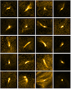 |
Fig. B.1. Additional examples of close-up view of 20 EUV brightenings. The FoV of each panel is 4 Mm×4 Mm. |
Appendix C: Distribution of properties of EUV brightenings for dataset-2
Figures C.1 and C.2 respectively show the histograms and scatter-plots for the properties of EUV brightenings for dataset-2. The corresponding figures for dataset-1 are shown as figs. 4 and 5 in Sect. 3.3. The trends in the different probability distributions and interrelation among different properties of the EUV brightenings are very similar for both the datasets, that are explained in Sect. 3.3.
All Figures
|
Fig. 1. Representative images of both EUI quiet-Sun observations studied in this article. Panels a and b show the visualisation from JHelioviewer (Müller et al. 2017), where the EUI/FSI 17.4 nm images overlaid with the near-simultaneous HRIEUV images are shown. The time mentioned in UTC corresponds to the time of observation at the Solar Orbiter. Carrington coordinates are shown, the crossing of the two yellow great circles indicates the antipode of the Earth/SDO sub-solar point. The red and blue markers indicate the solar north and south poles. Panels c and d show the HRIEUV images that cover a FoV of approximately 20° in longitude and latitude, corresponding to 215 Mm × 215 Mm on the surface of the Sun for both datasets. The detected EUV brightenings at the specific instance are marked in cyan over the respective FoVs for illustrative purposes. Movie 1 and movie 2 (available online) show the detected EUV brightenings over the full FoV for the complete duration of the two data-sequences. |
| In the text | |
|
Fig. 2. Illustrative examples of close-up view of six EUV brightenings. The FoV of each panel is 4 Mm × 4 Mm. |
| In the text | |
|
Fig. 3. Distributions of average brightness of EUV brightenings detected in the two datasets are shown in blue in each panel. Over-plotted are the respective distributions of pixel brightness of the temporally averaged FoV in grey. The overlapping region of the two distributions is shown in dark blue. The axes of both plots are shown with a log10 scale. |
| In the text | |
|
Fig. 4. Probability density distributions of properties of EUV brightenings for dataset-1. The probability density function (PDF) and power-law fit are shown for the distributions of surface area, lifetime, volume, and total intensity. The axes of all the plots are shown with a log10 scale. The corresponding figure for dataset-2 is shown in Appendix C. |
| In the text | |
|
Fig. 5. Relations between different properties of EUV brightenings for dataset-1. The scatter plot between surface area and lifetime is shown along with trends related to other morphological and photometrical properties in different panels. The axes of all the plots are shown with a log10 scale. The corresponding figure for dataset-2 is shown in Appendix C. |
| In the text | |
|
Fig. B.1. Additional examples of close-up view of 20 EUV brightenings. The FoV of each panel is 4 Mm×4 Mm. |
| In the text | |
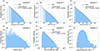 |
Fig. C.1. Same as Fig. 4 but for dataset-2. |
| In the text | |
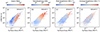 |
Fig. C.2. Same as Fig. 5 but for dataset-2. |
| In the text | |
Current usage metrics show cumulative count of Article Views (full-text article views including HTML views, PDF and ePub downloads, according to the available data) and Abstracts Views on Vision4Press platform.
Data correspond to usage on the plateform after 2015. The current usage metrics is available 48-96 hours after online publication and is updated daily on week days.
Initial download of the metrics may take a while.