| Issue |
A&A
Volume 686, June 2024
|
|
|---|---|---|
| Article Number | A17 | |
| Number of page(s) | 22 | |
| Section | Extragalactic astronomy | |
| DOI | https://doi.org/10.1051/0004-6361/202348559 | |
| Published online | 24 May 2024 | |
The transient event in NGC 1566 from 2017 to 2019
I. An eccentric accretion disk and a turbulent, disk-dominated broad-line region unveiled by double-peaked Ca II and O I lines⋆
1
Institut für Astrophysik und Geophysik, Universität Göttingen, Friedrich-Hund Platz 1, 37077 Göttingen, Germany
e-mail: This email address is being protected from spambots. You need JavaScript enabled to view it.
2
Ruhr University Bochum, Faculty of Physics and Astronomy, Astronomical Institute (AIRUB), 44780 Bochum, Germany
3
South African Astronomical Observatory, PO Box 9 Observatory Road, Observatory, 7935 Cape Town, South Africa
4
Southern African Large Telescope, PO Box 9 Observatory, 7935 Cape Town, South Africa
5
Department of Astronomy, University of Cape Town, Private Bag X3, Rondebosch 7701, South Africa
6
Department of Physics, University of the Free State, PO Box 339 Bloemfontein 9300, South Africa
7
Department of Physics, Faculty of Natural Sciences, University of Haifa, Haifa 3498838, Israel
8
Haifa Research Center for Theoretical Physics and Astrophysics, University of Haifa, Haifa 3498838, Israel
9
Nicolaus Copernicus Astronomical Center, Polish Academy of Sciences, Bartycka 18, 00-716 Warszawa, Poland
10
Universidad Católica del Norte, Instituto de Astronomía, Avenida Angamos 0610, Antofagasta, Chile
11
Department of Physics, Geology, and Engineering Technology, Northern Kentucky University, 1 Nunn Drive, Highland Heights, KY 41099, USA
12
School of Physics & Astronomy and the Wise Observatory, The Raymond and Beverly Sackler Faculty of Exact Sciences, Tel-Aviv University, Tel-Aviv 69978, Israel
13
Max-Planck-Institut für Radioastronomie, Auf dem Hügel 69, 53121 Bonn, Germany
14
Institute of Astronomy, Madingley Road, Cambridge CB3 0HA, UK
15
European Space Agency (ESA), European Space Astronomy Centre (ESAC), Villanueva de la Cañada, 28691 Madrid, Spain
Received:
10
November
2023
Accepted:
16
February
2024
Abstract
Context. NGC 1566 is a local face-on Seyfert galaxy and is known for exhibiting recurrent outbursts that are accompanied by changes in spectral type. The most recent transient event occurred from 2017 to 2019 and was reported to be accompanied by a change in Seyfert classification from Seyfert 1.8 to Seyfert 1.2.
Aims. We aim to study the transient event in detail by analyzing the variations in the optical broad-line profiles. In particular, we intend to determine the structure and kinematics of the broad-line region.
Methods. We analyzed data from an optical spectroscopic variability campaign of NGC 1566 taken with the 9.2 m Southern African Large Telescope (SALT) between July 2018 and October 2019 triggered by the detection of hard X-ray emission in June 2018. We supplemented this data set with optical to near-infrared (NIR) spectroscopic archival data taken by VLT/MUSE in September 2015 and October 2017, and investigated the emission from different line species during the event.
Results. NGC 1566 exhibits pronounced spectral changes during the transient event. We observe the emergence and fading of a strong power-law-like blue continuum as well as strong variations in the Balmer, He I, and He II lines and the coronal lines [Fe VII], [Fe X], and [Fe XI]. Moreover, we detect broad double-peaked emission line profiles of O Iλ8446 and the Ca IIλλ8498, 8542, 8662 triplet. This is the first time that genuine double-peaked O Iλ8446 and Ca IIλλ8498, 8542, 8662 emission in AGN is reported in the literature. All broad lines show a clear redward asymmetry with respect to their central wavelength and we find indications for a significant blueward drift of the total line profiles during the transient event. The profiles and the FWHM of the Balmer lines remain largely constant during all observations. We show that the double-peaked emission line profiles are well approximated by emission from a low-inclination, relativistic eccentric accretion disk, and that single-peaked profiles can be obtained by broadening due to scale-height-dependent turbulence. Small-scale features in the O I and Ca II lines suggest the presence of inhomogeneities in the broad-line region.
Conclusions. We conclude that the broad-line region in NGC 1566 is dominated by the kinematics of a relativistic eccentric accretion disk. The broad-line region can be modeled to be vertically stratified with respect to scale-height turbulence with O I and Ca II being emitted close to the disk in a region with high (column) density, while the Balmer and helium lines are emitted at greater scale height above the disk. The observed blueward drift might be attributed to a low-optical-depth wind launched during the transient event. Except for this wind, the observed kinematics of the broad-line region remain largely unchanged during the transient event.
Key words: galaxies: active / galaxies: Seyfert / galaxies: nuclei / quasars: individual: NGC 1566 / quasars: emission lines
Based on observations made with the Southern African Large Telescope (SALT).
© The Authors 2024
 Open Access article, published by EDP Sciences, under the terms of the Creative Commons Attribution License (https://creativecommons.org/licenses/by/4.0), which permits unrestricted use, distribution, and reproduction in any medium, provided the original work is properly cited.
This article is published in open access under the Subscribe to Open model. This email address is being protected from spambots. You need JavaScript enabled to view it. to support open access publication.
1. Introduction
Variability is widespread in active galactic nuclei (AGN). It occurs in all spectral bands and on typical timescales of hours to weeks or even years. Generally, the variability of AGN is assumed to be stochastic in nature and has been used with great success in the last ∼30 years to identify and map the innermost AGN structures – namely the accretion disk (AD), the broad-line region (BLR), and the dusty torus (TOR) – using methods such as reverberation mapping (RM; Blandford & McKee 1982). RM traces the lagging emissive response of individual AGN emission lines to the time-varying ionizing continuum radiation from the central source close to the supermassive black hole (SMBH). As regular and densely sampled observations of the X-ray/UV ionizing continuum are difficult to acquire, an optical continuum is often used as a proxy for the ionizing radiation. Typical optical continuum and line variability for an object (on timescales of months) can span a wide range, from only a few percent up to a few dozen percent (e.g., Ulrich et al. 1997). Aside from these typical temporal variations of the continuum and emission lines, studies have shown that the variability behavior of individual objects can differ from one epoch to another, and apparent variations of the BLR responsivity have been reported (e.g., Hu et al. 2020; Gaskell et al. 2021), sometimes over timescales comparable to or even shorter than the expected dynamical timescales (De Rosa et al. 2018).
In addition to the overall stochastic variability behavior of AGN, transient events such as changing-look (CL) transitions have increasingly gained attention over recent years. Originally, the term “changing-look” was used to describe Compton-thick AGN becoming Compton-thin and vice versa (e.g., Guainazzi 2002; Matt et al. 2003). In analogy, optical CL AGN are characterized by their change of spectral classification, switching between Sy 1 and Sy 2 and associated subtypes1. These transitions happen over timescales of months to years and are often accompanied by significant flux changes on the order of several magnitudes (e.g., MacLeod et al. 2016; Graham et al. 2020; Green et al. 2022). The observed change between Seyfert types during CL events does not challenge the general validity of the unified AGN model, according to which the source classification is mainly due to the orientation with respect to the observer (Antonucci 1993). Rather, the huge change in continuum flux on short timescales and the resulting apparent changes in BLR kinematics provide a unique opportunity to refine our understanding of BLR structure. According to the locally optimized cloud model (LOC model, Baldwin et al. 1995), the continuum luminosity determines which parts of the BLR – near or far from the continuum source – are visible. If the BLR is not scale invariant, then a transient event inevitably leads to obvious changes in BLR kinematics and Seyfert subtype. However, to date, the implications of the LOC model have not been adequately addressed in CL-AGN research.
The typical CL transition timescales cannot be explained by viscous radial inflow, a circumstance that is known as the “viscosity crisis” (Lawrence 2018, and references therein). Currently, several explanations for the CL phenomenon are discussed, including tidal disruption events (TDEs), strong variations in the accretion flow, microlensing caused by an intervening object, or sudden changes in obscuration. However, at least for some cases, the behavior of the observed post-CL light curves disfavors discrete events as the cause of the CL phenomenon (e.g., Runnoe et al. 2016; Zetzl et al. 2018). In general, the similarities between TDEs and some observed CL events require clearly defined distinction criteria and, in turn, extensive observational data for each event (e.g., Zabludoff et al. 2021; Komossa & Grupe 2023).
Other possible mechanisms that are discussed include accretion disk instabilities (Nicastro et al. 2003), magneto-rotational instabilities (e.g., Ross et al. 2018), radiation pressure instabilities (Śniegowska et al. 2023), magnetically elevated accretion (e.g., Dexter & Begelman 2019), accretion state transitions (e.g., Noda & Done 2018), and interactions between binaries of SMBHs (Wang & Bon 2020). In addition, the phenomenon of periodicities in AGN light curves (e.g., Bon et al. 2017, and references therein) and repeat CL events (e.g., Sniegowska et al. 2020) has gained more attention from the scientific community in recent years.
Until recently, CL events were thought to be rather rare. However, the evidence for CL events being much more common has been growing in recent years. To date, a few dozen CL AGN have been identified. Early detections include NGC 1566 (Pastoriza & Gerola 1970), NGC 3515 (Collin-Souffrin et al. 1973), NGC 4151 (Penston & Perez 1984), and Fairall 9 (Kollatschny & Fricke 1985). More recent detections are, for example, NGC 2617 (Shappee et al. 2014), Mrk 590 (Denney et al. 2014), HE 1136–2304 (Parker et al. 2016; Zetzl et al. 2018; Kollatschny et al. 2018), WISE J1052+1519 (Stern et al. 2018), and 1ES 1927+654 (Trakhtenbrot et al. 2019a). However, only a few of them – most notably 1ES 1927+654 – have been studied spectroscopically in greater detail in temporal proximity to the transient event. This lack of high-quality data is a significant hinderance to endeavors to understand the CL phenomenon.
NGC 1566 (α2000 = 04h 20m 00.42s, δ2000 = −54 ° 56′ 16.1″) is a local (z = 0.00502) face-on Seyfert galaxy2 and is known for exhibiting recurrent outbursts accompanied by changes in spectral type (Shobbrook 1966; Pastoriza & Gerola 1970; Alloin et al. 1985, 1986). The most recent transient event occurred from 2017 to 2019, and an accompanying CL event (a change in Seyfert classification from Sy 1.8 to Sy 1.2; that is, from showing only weak broad emission in Hβ and Hα to showing stronger broad Hβ emission) was reported by Oknyansky et al. (2019, 2020). Optical (post-)outburst spectra from 2018 were presented by Oknyansky et al. (2019, 2020) and Ochmann et al. (2020). The flux and spectral variations were the strongest changes observed since 1962, when NGC 1566 exhibited similarly strong broad-line emission (Shobbrook 1966; Pastoriza & Gerola 1970). The object already started to brighten significantly in September 2017 (Dai et al. 2018) and reached its peak optical flux in July 2018. A thorough historical overview of the variations in NGC 1566 from the 1960s until today can be found in Oknyansky et al. (2020).
Here, we present first results of a multiwavelength campaign of NGC 1566 during its transient event from 2017 to 2019. Observations with SALT, XMM-Newton, NuSTAR, and Swift were triggered by the detection of hard X-ray emission with Integral in June 2018 (Ducci et al. 2018). This led to a dense multiwavelength campaign with a duration of ∼850 days and follow-up observations in 2019/2020. The first XMM-Newton, NuSTAR, and Swift observations (Parker et al. 2019) revealed the rapid increase in X-rays and the presence of a typical Seyfert-1-type X-ray spectrum in outburst, along with the formation of an X-ray wind at v ∼ 500 km s−1. In 2023 October, NGC 1566 was found to be in a low state in all Swift bands (Xu et al. 2024). Further results of the observations with XMM-Newton, NuSTAR, and Swift will be presented in future publications. Our observations are supplemented by archival observations with VLT/MUSE, and cover the optical and NIR wavelength range (∼4300 Å–∼9300 Å) at epochs directly before, during, and after the transient event. The observations in detail reveal drastic changes in the line emission and nonstellar continuum. The present paper is structured as follows. In Sect. 2, we describe the observations and the data reduction. In Sect. 3, we present the analysis of the spectroscopic observations. We discuss the results in Sect. 4 and summarize them in Sect. 5. Throughout this paper, we assume a Λ cold dark matter cosmology with a Hubble constant of H0 = 73 km s−1 Mpc−1, ΩΛ = 0.73, and ΩM = 0.27.
2. Observations and data reduction
2.1. Optical spectroscopy with SALT
We acquired optical long-slit spectra of NGC 1566 with the Southern African Large Telescope (SALT; Buckley et al. 2006) at 2 epochs shortly after the detection of hard X-ray emission in June 2018, and one follow-up spectrum in September 2019. The observations have proposal codes 2018-1-DDT-004, 2018-1-DDT-008 (PI: Kollatschny) and 2018-2-LSP-001 (PI: Buckley). The log of the spectroscopic observations is given in Table 1. In addition to the galaxy spectra, we took necessary calibration images (flat-fields, Xe arc frames). All observations were taken under identical instrumental conditions with the help of the Robert Stobie Spectrograph (RSS; Kobulnicky et al. 2003) using the PG0900 grating and a 2 × 2 spectroscopic binning. To minimize differential refraction, the slit width was fixed to  projected onto the sky at an optimized projection angle. For the extraction of the spectra, we used a square aperture of
  ×
×  . We covered the wavelength range from 4210 to 7247 Å with a spectral resolution of ∼6.7 Å. This corresponds to object rest-frame wavelengths of 4189 to 7211 Å. Two gaps in the spectra are caused by gaps between the three CCDs of the spectrograph. They range from 5219 to 5274 Å and 6262 to 6315 Å (5193 to 5248 Å and 6231 to 6283 Å in the rest-frame), respectively. For all observations, we used the same instrumental setup as well as the same standard star (LTT 4364) for flux calibration, and performed standard reduction procedures using IRAF packages. In order to account for small spectral shifts (≲0.5 Å) in the wavelength calibration between spectra, we performed a wavelength intercalibration with respect to the MUSE spectra. This was done separately for the Hβ and Hα line using the narrow lines [O III] λλ4959, 5007 and [S II] λλ6716, 6731, respectively.
Log of spectroscopic observations of NGC 1566 before, during and after the transient event in 2018.
In addition to our three observations, we utilize one additional SALT observation of NGC 1566 from the SALT archive3 for our variability study. This spectrum was taken on 2018 July 30 as part of the proposal 2018-1-SCI-029 (PI: Marchetti) by the RSS using the PG0900 grating, a  slit and 2 × 4 binning. This setup covered the wavelength range from 4920 to 7922 Å with a spectral resolution of ∼5.7 Å. This corresponds to object rest-frame wavelengths of 4895 to 7882 Å. We followed the same reduction steps as for the other SALT observations, employing calibration images with matching instrumental setup. In particular, we used the same standard star LTT 4364 for flux calibration of the spectrum. The signal-to-noise ratio (S/N) in the continuum range (5100 ± 20) Å (rest-frame) is ∼110 compared to S/N ∼190 in the
  aperture SALT spectrum from 2018 July 20.
All spectra were corrected for Galactic reddening applying the extinction curve of Cardelli et al. (1989) and using a ratio R of absolute extinction A(V) to EB − V = 0.0079 (Schlafly & Finkbeiner 2011) of 3.1, and calibrated to the same [O III] λ5007 flux of (102 ± 2)×10−15 ergs s−1 cm−2 (see Sect. 2.2) in the optical regime. We also corrected for slightly different background flux contributions between observations using an intercalibration to a campaign (Ochmann et al., in prep.) with the UV-Optical Telescope (UVOT; Roming et al. 2005) of Swift. The differing background flux contributions arise due to differing observing conditions between observations and the large spatial extent of NGC 1566 in the slit.
2.2. Optical and NIR spectroscopy with MUSE
NGC 1566 was observed with VLT/MUSE (Multi Unit Spectroscopic Explorer; Bacon et al. 2010, 2014) IFU spectrograph as part of the ESO programs 096.D-0263 (PI: J. Lyman) and 0100.B-0116 (PI: C. M. Carollo) on 2015 September 24 and 2017 October 23, respectively. The former observation was carried out in the no-AO wide field mode (WFM), that is, with natural seeing and FoV of 1′×1′, while the latter was performed in the AO WFM making use of adaptive optics. MUSE covers the optical and NIR wavelength range between ∼4700 Å and 9300 Å at a spectral resolution of ∼2.5 Å. The spectra are sampled at 1.25 Å in dispersion direction and at  in spatial direction. The seeing and exposure time of the observations are given in Table 1.
The data were reduced using the MUSE pipeline development version 1.6.1 and 2.2 (Weilbacher et al. 2012, 2014) for the observation from 2015 September 24 and 2017 October 23, respectively. This reduction includes the usual steps of bias subtraction, flat-fielding using a lamp-flat, wavelength calibration and twilight sky correction. Every data cube is the product of four combined raw science images. We extracted spectra of NGC 1566’s nucleus and the H II region detected by da Silva et al. (2017) using circular apertures of  and
and  radius, respectively. The apertures were chosen such that they are centered on the respective region, comprise the bulk of the emission, and have minimal overlap. A zoomed-in region of the data cube from 2017 October 23 centered on the nucleus is shown in Fig. 1. The apertures are indicated by a blue and magenta circle, respectively.
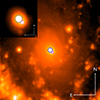 |
Fig. 1. Image ( |


In the following, we use the AO wide field mode MUSE spectrum from 2017 October 23 as a reference spectrum for all spectroscopic observations. Therefore, we calibrated all spectra to the same absolute [O III] λ5007 flux of (102 ± 2)×10−15 ergs s−1 cm−2. This value is in agreement with results of Kriss et al. (1991), who measured an [O III] λ5007 flux of (101.62 ± 7.32)×10−15 ergs s−1 cm−2 in a HST/FOS spectrum obtained with an aperture of  on 1991 February 8. This indicates that the bulk of the [O III] λ5007 emission close to the nucleus stems from a confined region with a size
  , which translates to ≲30 pc using the Cosmology Calculator of Wright (2006).
3. Results
3.1. Optical spectral observations
We present all reduced optical spectra obtained before, during, and after the transient event in NGC 1566 in Fig. 2. For each spectrum, we give a chronologically sorted ID, the UT date and the time difference in days with respect to 2018 July 2 (t0 = 58301.44 MJD), when NGC 1566 reached its peak optical flux in the ASAS-SN4 (All-Sky Automated Survey for SuperNovae; Shappee et al. 2014; Kochanek et al. 2017; Jayasinghe et al. 2019) V-band and g-band light curves.
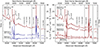 |
Fig. 2. All optical spectra obtained before, during, and after the transient event in NGC 1566. MUSE and SALT spectra are shown in blue and red, respectively. The left panel shows the spectra obtained during the rising phase, including the optical spectrum from 2018 July 20, while the right panel shows the spectra obtained during the declining phase, again including the optical high-state spectrum from 2018 July 20 for reference. The SALT spectrum from 2018 July 30 is shifted by −2 × 10⁻¹⁵ ergs s−1 cm−2 Å−1 for clarity. For each spectrum, we give the ID as well as the UT date of the observation. The most prominent telluric absorption bands are flagged (gray). |
Spectrum 1 was obtained on 2015 September 24, and therefore ∼700 days before Dai et al. (2018) reported a brightening of NGC 1566 in September 2017, and 1012 days before the transient event reached its peak. Spectrum 25 was obtained on 2017 October 23, 252 days before peak flux. This spectrum sees the emergence of a nearly linear continuum across the optical band, accompanied by the appearance of strong Fe II multiplet emission of the transitions 42 (∼4910 − 5180 Å), 48 and 49 (∼5185 − 5450 Å), and weak coronal line emission of [Fe VII] λλ5721, 6087 and [Fe X] λ6375 as well as weak emission of He Iλλ6678, 7065.
Spectra 3 and 4 were obtained on 2018 July 20 and July 30, and therefore 18 and 28 days after peak flux. Spectrum 3 has already been presented by Ochmann et al. (2020), however, it had not been intercalibrated to the other spectra of the campaign (see Sect. 2.1). To our knowledge, these two high-state spectra presented here are the optical spectra closest to the transient peak presented in the literature so far (see Oknyansky et al. 2019, 2020). The two spectra are qualitatively identical and show a strong, power-law-like blue continuum, broad He Iλλ5876, 6678, 7065 emission, strong emission in Hα, very prominent emission between ∼5100 Å and ∼5700 Å, usually attributed to Fe II emission, as well as coronal line emission of [Fe VII] λλ5721, 6087 and [Fe X] λ6375. Due to the larger wavelength coverage, Spectrum 3 also reveals strong emission of the Balmer lines Hγ and Hβ as well as of He IIλ4686 and the Fe II multiplet transitions 38 and 39 (∼4500 − 4650 Å).
Spectra 5 and 6 were obtained 95 and 434 days after the transient peak, respectively, and reveal the fading of the strong blue continuum as well as of the broad emission lines. One notable exception from the general fading are the coronal lines [Fe VII] λλ5721, 6087, which are stronger in the spectrum from 2018 October 4 than in the high-state spectra obtained 77 and 67 days earlier. The spectrum from 2019 September 9 is approximately on the same level as the low-state spectrum from 2015 September 24, but still shows a slightly stronger continuum blueward of ∼6000 Å.
To illustrate the timing of the spectral observations, we show the time stamps of all spectral observations along with the ultraviolet Swift UVW2-band light curve in Fig. 3. Further, more detailed results on the spectral variations in NGC 1566 during its transient event from 2017 to 2019 will be presented in future publications (Kollatschny et al., in prep.; Ochmann et al., in prep.).
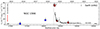 |
Fig. 3. Long-term UV Swift UVW2-band light curve before, during, and after the transient event in NGC 1566 from 2017 to 2019. The blue and red boxes mark the time stamps of the spectroscopic MUSE and SALT observations, respectively, and are numbered chronologically. To guide the eye, the boxes are positioned such that they overlap with the UVW2 light curve; that is to say, they do not represent the actual optical flux values, but give a basic representation of the relative flux with respect to each other. The date of detection of the supernova ASASSN-14ha is indicated by a red arrow and the date of peak flux in the ASAS-SN light curve is shown by a gray line. The pretransient low-state flux level is indicated by a dashed black line. |
3.1.1. Host galaxy contribution
All spectra of NGC 1566 (see Fig. 2) show a strong stellar signature from the underlying host galaxy. This holds especially true for the low-state spectra before and after the outburst, where the stellar signature of the host galaxy clearly dominates the continuum regions of the spectra. In order to determine the host galaxy contribution, we perform a spectral synthesis on Spectrum 1 from 2015 September 24. Of all the spectra in the campaign, this spectrum is the most suitable as it has the largest spectral coverage from ∼4700 Å to 9300 Å and the lowest contribution from broad-line emission and nonstellar continuum. The way we proceed is identical to that presented for IRAS 23226−3843 by Kollatschny et al. (2023). We use the Penalized Pixel-Fitting method (pPXF; Cappellari & Emsellem 2004; Cappellari 2017) and restrict the synthesis to wavelength ranges free from emission lines. This excludes in particular the Fe II complex at ∼5300 Å from the fitting procedure. We used the stellar templates from the Indo-US library (Valdes et al. 2004; Shetty & Cappellari 2015; Guérou et al. 2017), which provides high-enough spectral resolution, and fully covers the wavelength range of interest. In addition to the stellar templates, we add a constant component Fλ = c mimicking a very weak power-law component Fλ ∝ λ−β as the underlying nonstellar AGN continuum. This seems to us to be a reasonable estimate, since we cannot make an a priori statement about the nonstellar spectral index in the low-state spectrum and the contribution of a very weak power law can be approximated as constant in the optical regime6.
The result of the spectral synthesis is shown in Fig. 4 together with the input spectrum and the residual spectrum, which is the clean nuclear spectrum of NGC 1566 during its low state. The residual spectrum already includes the approximately constant nonstellar AGN component Fλ = 1.4 × 10⁻¹⁵ ergs s−1 cm−2 Å−1. This allows us to estimate the host galaxy contribution in the original low-state spectrum to be ∼60% and ∼70% in the B and V band, respectively. The clean low-state nuclear spectrum reveals line features formerly suppressed by the signature of the stellar population in the original spectrum. These features include, amongst others, narrow-line emission of [N I] λ5198, Fe II emission of the transitions 42, 48, and 49, weak He Iλλ5876, 6678, 7065 emission, and Ca IIλλ8498, 8542, 8662 triplet emission, as well as emission of O Iλ8446.
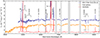 |
Fig. 4. MUSE spectrum of NGC 1566 taken on 2015 September 24 (Spectrum 1; blue) and the synthesis fit of the stellar contribution with pPXF (orange). The residuals (red) give the clean nuclear emission lines spectrum. For the fit, we flagged all prominent line emission including the Fe II complex at ∼5300 Å. The most prominent telluric absorption bands are flagged (gray). |
pPXF determines a stellar velocity dispersion of  km s−1. The exact value depends on the choice of the boundary conditions, namely the inclusion or exclusion of the NIR Ca II triplet and the probed wavelength region. We determined the error margins by reasonably varying the boundary conditions, that is, slighty varying the probed wavelength regions (±50 Å), probing only the optical or NIR part, and exluding or including the NIR Ca II triplet, thereby obtaining a robust range of variation for σ*. We note that the MUSE spectrum from 2017 October 23, although obtained under favorable seeing conditions, is not suitable to determine an estimation σ*. In this spectrum, the most prominent absorption feature, namely the Ca II absorption triplet, is blended with Ca II emission, and many wavelength bands are affected by newly emerging line emission (see Sects. 3.1 and 3.2). This limits the spectral range with a clean host-galaxy signature and introduces a large scatter in the distribution of determined stellar velocity dispersions σ*.
3.1.2. Balmer line profiles and their evolution
In order to obtain clean nuclear line profiles, we subtract the synthetic host-galaxy spectrum (see Sect. 3.1.1) from each spectrum after correcting all spectra to the same dispersion. The resulting host-free, singular-epoch line profiles of Hβ and Hα are shown in Fig. 5, where we indicate the central wavelength of Hβ and Hα with a dashed line. In order to show the accuracy of the wavelength calibration, which is on the order of ±20 km s−1, we likewise indicate the central wavelengths of [O III] λ4959, 5007 and [S II] λλ6716, 6731, respectively. Both the Hβ and the Hα profiles show a pronounced redward asymmetry during all phases of the transient event, with no major changes in the overall line profile. This was also observed by Alloin et al. (1985), who found the same redward asymmetry and no significant line profile variations despite considerable flux changes during their optical variability campaign of NGC 1566 from 1980 to 1982. Kriss et al. (1991) reported redshifts of 200 − 1000 km s−1 for all broad lines in their UV to optical FOS/HST spectra.
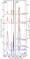 |
Fig. 5. Temporal evolution (from bottom to top) of the host-free line profiles of Hβ (left panel) and Hα (right panel). MUSE spectra are shown in blue, SALT spectra are shown in red. The profiles are shifted in flux for clarity. We indicate the central wavelengths of Hβ and Hα by dashed lines. Likewise, we indicate the central wavelengths of the narrow lines [O III] λ4959, 5007 and [S II] λλ6716, 6731 to demonstrate the accuracy of the spectral calibration. |
In order to assess the line profile variations of Hβ and Hα in more detail, we calculate the host-free mean and rms line profiles. The resulting profiles are shown in Fig. 6. The Hβ and Hα rms profiles, which map only the variable part of the line emission, show no evidence of residual narrow-line flux from Hβnarrow, [O III] λλ4959, 5007 (see also Sect. 3.3) and Hαnarrow, [N II] λλ6548, 6583, respectively. This illustrates the high accuracy of the spectral intercalibration. The profiles have a FWHM of (2180 ± 50) km s−1 and (2060 ± 50) km s−1 for Hβ and Hα, respectively, and are strongly asymmetric with respect to the rest-frame velocity, with the red wing being broader by about ∼400 km s−1 with respect to the central wavelength. In addition, both rms profiles show an additional narrow peak component that is not associated with narrow-line residuals, but instead is shifted with respect to the rest-frame central wavelength by (220 ± 50) km s−1 and (210 ± 50) km s−1, respectively. With respect to the peak positions, the central rms profiles are almost perfectly symmetric. Major deviations from symmetry are only evident in the extended line wings.
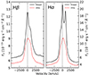 |
Fig. 6. Mean (solid black) and rms (dashed red) line profiles of Hβ (left panel) and Hα (right panel). The central velocity v = 0 km s−1 is indicated by a black dashed line. The Hβ and Hα rms profiles show a peak at +(220 ± 50) km s−1 and +(210 ± 50) km s−1, respectively, with respect to the central wavelength. The profiles are strongly asymmetric with the red wing being broader by about ∼400 km s−1. The FWHM amounts to (2180 ± 50) km s−1 and (2060 ± 50) km s−1 for Hβ and Hα, respectively. |
At this point, the individual Hβ and Hα line profiles still comprise contributions from the narrow components Hβnarrow and Hαnarrow as well as [N II] λλ6548, 6583, respectively. Therefore, in order to obtain clean FWHM measurements for singular epochs, we subtract a scaled [O III] λ5007 profile taken from the 2015 September 24 spectrum as a mean template for each narrow-line component from the total line profile. We adopt this procedure as we explicitly assume that the narrow-line components are not purely Gaussian, but instead are more complex as they are being shaped by the kinematics of the narrow-line region. This is supported by the findings of Alloin et al. (1985) and da Silva et al. (2017), who found that adequately modeling the narrow lines in NGC 1566 requires at least two Gaussians.
We show the resulting broad Hβ line profiles after subtraction of a suitable linear pseudo-continuum in Fig. 7. From each of these profiles, we subtracted a constant narrow-line component Hβnarrow with a flux of 18.2 × 10⁻¹⁵ ergs s−1 cm−2. We give the measured FWHM and redshift of all Hβbroad profiles in Table 2. We observe the following trends in the emission lines: The Hβ profiles in Spectrum 1, Spectrum 2 and Spectrum 3 are skewed and clearly display the redward asymmetry mentioned previously. While the Hβbroad profile in Spectrum 1 exhibits minor distortions of the central profile, probably due Hβnarrow residuals (see also Sect. 3.3), the profile in Spectrum 2 appears to be free from this effect. Most strikingly, we observe a substantial change in redshift of the Hβbroad profile between Spectrum 1 and Spectrum 2, with a shift of the line peak from +(730 ± 50) km s−1 to +(490 ± 50) km s−1. This trend continues until Spectrum 3, where the redshift of the profile only amounts to +(360 ± 50) km s−1. We term this velocity shift of the total Hβ profile during the rising phase of the transient event to be a blueward drift of the line profile. To illustrate we show the normalized Hβ profiles from Spectrum 1 to Spectrum 3 in Fig. 8.
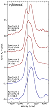 |
Fig. 7. Temporal evolution (from bottom to top) of the normalized, narrow-line, and host-galaxy-subtracted Hβ profiles in velocity space. A suitable linear pseudo-continuum was subtracted, and the spectra are flux-shifted for clarity. MUSE spectra are shown in blue, SALT spectra are shown in red. The central velocity v = 0 km s−1 is indicated by a dashed line. We give the spectrum ID, the date of observations, and the time in days with respect to the peak time t0 = 58301.44 MJD of the transient event. The reconstructed Hβ profile for Spectrum 1 (2015 September 24) is shown as a dotted line (see Sect. 3.3). |
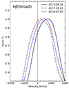 |
Fig. 8. Blueward drift of the normalized Hβ profiles in velocity space (from Spectrum 1 (2015 September 24) to Spectrum 2 (2017 October 23), and Spectrum 3 (2018 July 20)) after subtraction of the narrow-line and the host-galaxy contribution. The Hβ profile from Spectrum 1 is the reconstructed Hβ profile (see Sect. 3.3). The blueward drift of the Hβ profile during the rising phase is clearly visible. The redshift of the Hβ line shifts from +(730 ± 50) km s−1 to +(490 ± 50) km s−1 and +(360 ± 50) km s−1 from Spectrum 1 to Spectrum 2 and Spectrum 3, respectively. |
FWHM and redshift Δv (with respect to the central wavelength) of the Hβ line profile for all epochs.
In comparison to the Hβ profiles from Spectrum 1 to Spectrum 3, the Hβ profile in Spectrum 5 is slightly distorted with an apparent additional emission component at +(130 ± 10) km s−1. The redshift increases from +(360 ± 50) km s−1 to +(450 ± 100) km s−1 from Spectrum 3 to Spectrum 5. The profile in Spectrum 6 is two-peaked, caused by the apparent emission component in Spectrum 5 now being present as an apparent absorption component that distorts the profile. Due to the absorption, the Hβbroad profile cannot be normalized to peak height like the previous profiles, and no meaningful measurement of the redshift can be performed.
Strikingly, the profile and the FWHM of Hβbroad do not change significantly during the rising phase of the transient event. The slightly lower value of FWHM = (1970 ± 50) km s−1 in the low-state Spectrum 1 from 2015 September 24 compared to the other spectra is caused by the minor distortion of the central profile due to a narrow-line residual. Taking this residual into account (see Sect. 3.3), the width amounts to FWHM = (2200 ± 50) km s−1, and is therefore in perfect agreement with the values obtained for the other profiles7.
Although our procedure is able to recover clean Hβbroad profiles, it is not successful in recovering Hαbroad profiles. This is due to differences in the exact profile shape and width between [O III] λ5007 and [N II] λλ6548, 6583. Nevertheless, because of the very similar rms profiles of both Hβ and Hα, we suspect Hαbroad to show the same behavior as Hβbroad.
3.1.3. Black hole mass estimation using the MBH − σ* and MBH–FWHM(Hβ), L5100 scaling relations
In Sect. 3.1.1, we obtain a value of  km s−1 for the stellar velocity dispersion in the nuclear region of NGC 1566 during its low state. For the same spectrum we obtain a clean measurement of FWHM(Hβ) = (2200 ± 50) km s−1 in Sect. 3.1.2. These results allow us to estimate the black hole mass MBH using the MBH − σ* scaling relation of Onken et al. (2004, see their Eq. (2)) and the MBH–FWHM(Hβ), L5100 scaling relation of Vestergaard & Peterson (2006, see their Eq. (5)). From the MBH − σ* scaling relation we obtain
 (1)
(1)
For the MBH–FWHM(Hβ), L5100 scaling relation, we measure L5100 in the host-free low-state spectrum. We obtain a continuum flux of Fλ = 1.4 × 10⁻¹⁵ ergs s−1 cm−2 Å−1, which results in a luminosity of λL5100 = 3.91 × 1041 ergs s−1. Together with FWHM(Hβ) = (2200 ± 50) km s−1 measured in Sect. 3.1.2, we therefore obtain a black hole mass of
 (2)
(2)
Using a velocity dispersion of σ* = (105 ± 10) km s−1, which is slightly higher than  km s−1 obtained by us, Smajić et al. (2015) obtained a mass of MBH = (8.6 ± 4.4)×106 M⊙. Using also the flux and FWHM of broad Br γ from their data, they estimated the black hole mass MBH in NGC 1566 to be MBH = (3.0 ± 0.9)×106 M⊙, and found their results to be in good agreement with results obtained by Woo & Urry (2002) and Kriss et al. (1991), respectively. We give their results and our values in Table 3. From here on, we adopt the mean black hole mass of MSMBH = (5.3 ± 2.7)×106 M⊙ for NGC 1566.
Black hole masses MSMBH for NGC 1566 determined by different studies.
3.2. Near-infrared spectral observations
MUSE observed NGC 1566 on 2015 September 24 and 2017 October 23 in the wavelength range ∼4700 Å to 9300 Å. This is ∼700 days before and ∼50 days after the start of the reported brightening of NGC 1566 in September 2017, respectively. We show the NIR part (rest-frame wavelength 7000 Å–9300 Å) of the nuclear spectra together with the resulting difference spectrum in Fig. 9. The spectra were extracted using a circular aperture with a radius of 1″. In contrast to the optical regime, the spectra are intercalibrated to the same narrow-line flux of [O II] λλ7320, 7330, [Ni II] λ7378, and [S III] λ9069, as well as the same absorption strength in the Ca IIλλ8498, 8542, 8662 triplet. The absorption strength of the Ca II triplet can be considered constant due to the identical aperture of both observations, in other words, the underlying stellar population from the host galaxy is identical.
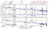 |
Fig. 9. Intercalibrated MUSE NIR spectra from 2015 September 24 and 2017 October 23 (upper panel) and the resulting difference spectrum (lower panel). The most prominent telluric absorption bands are shown in gray. In addition to an increase in NIR continuum flux, the difference spectrum reveals emission from several broad lines and [Fe XI] λ7892. The most prominent emission feature is the blend of O Iλ8446 and the Ca IIλλ8498, 8542, 8662 triplet (gray box). The linear pseudo-continuum used for later analysis is shown as a gray line. The positions of all identified emission lines are marked by dashed lines. Narrow emission lines and the stellar Ca II triplet absorption are denoted in black, while variable line emission is denoted in red. |
Spectrum 1 from 2015 September 24 is clearly dominated by the stellar contribution from the host galaxy. The most prominent emission feature in this spectrum are the narrow lines [O II] λλ7320, 7330, [Ni II] λ7378 and [S III] λ9069. In addition, prominent absorption in the Ca IIλλ8498, 8542, 8662 triplet is present. Spectrum 2 from 2017 October 23, approximately 50 days into the brightening, shows the emergence of a nearly linear continuum across the entire wavelength band, as well as several additional emission lines. Both continuum and line flux can be best recognized in the difference spectrum. We identify broad emission from He Iλ7065, possible emission from Pa 12 λ8751, Pa 11 λ8863 (although only marginally detected in both cases) and Pa 9 λ9229, as well as emission from the coronal line [Fe XI] λ7892, all of which previously not present in the low-state spectrum from 2015 September 24. In addition to the lines identified before, we observe the emergence of broad emission at ∼7306 Å, which cannot be unambiguously identified. This broad-line feature might also be present in other NIR AGN spectra (e.g., Landt et al. 2008), however, a clear detection in singular-epoch spectra is difficult due to blending with the narrow lines [O II] λλ7320, 7330.
The most prominent emission feature is broad emission in O Iλ8446 and the Ca IIλλ8498, 8542, 8662 triplet. We indicate these lines in Fig. 9 by a gray box. The linear continuum subtracted from the line profiles for further analysis is shown by a gray line. A thorough analysis of the line profiles is performed in Sects. 3.2.1–3.2.3. We show that the Ca IIλ8662 profile is well approximated by emission from an elliptical disk. Furthermore, the blended total profile of O Iλ8446 and Ca IIλλ8498, 8542 can be reconstructed using the Ca IIλ8662 difference profile as a template for all three lines.
3.2.1. The double-peaked Ca II λ8662 line profile
We show the clean line profile of Ca IIλ8662 in velocity space (after subtraction of the underlying linear continuum indicated in Fig. 9) in Fig. 10. The Ca IIλ8662 difference profile is double-peaked, with the red peak being stronger than the blue peak by about 10%. Moreover, the red peak is composed of three individual subpeaks that form a “trident” structure. The total profile is strongly asymmetric with the right wing being broader by ∼300 km s−1. The full width at half maximum (FWHM) amounts to (1920 ± 50) km s−1 when the Ca IIλ8662 profile is normalized to Fλ(0 km s−1) = 1. The blue and red peak are positioned at vblue peak ≈ −615 km s−1 and vred peak ≈ +950 km s−1, respectively, and are therefore separated by ∼1600 km s−1.
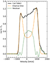 |
Fig. 10. Normalized difference line profile of Ca IIλ8662 in velocity space (black) after subtraction of a linear pseudo-continuum. The profile is double-peaked and strongly asymmetric, with the red peak being stronger (by about 10%) and being shifted to higher velocities (vred peak ≈ +950 km s−1) than the blue peak (vblue peak ≈ −615 km s−1). In addition, the red peak shows a “trident” structure, meaning, it is composed of three individual subpeaks. The width of the profile amounts to FWHM = (1920 ± 50) km s−1. We show the best-fit results for the elliptical disk model (orange) and the residual flux (green). |
The profile closely resembles that of H I 21 cm-line emission profiles in so-called “lopsided” galaxies, where the matter distribution in the galaxy’s plane is asymmetric with respect to the galaxy’s center (e.g., Richter & Sancisi 1994). Similar asymmetric line profiles have been observed in a number of AGN, for example, Arp 102B (Popović et al. 2014), NGC 4958 (Ricci & Steiner 2019), NGC 1097 (Storchi-Bergmann et al. 1997; Schimoia et al. 2015), and others (Gezari et al. 2007; Lewis et al. 2010), as well as TDEs, for example, PTF09djl (Liu et al. 2017), AT 2018hyz (Hung et al. 2020), AT 2020zso (Wevers et al. 2022), and are thought to be signatures of an elliptical (accretion) disk. We analyze the line profile of Ca IIλ8662 in the framework of an elliptical accretion disk model in Sect. 3.2.2 in more detail.
3.2.2. Fitting the Ca II λ8662 difference profile with an elliptical accretion disk model
The analysis of the Ca IIλ8662 difference profile reveals a strongly asymmetric, double-peaked profile with the red peak being stronger than the blue peak by about 10%. Emission line profiles with stronger red than blue peaks are inconsistent with circular accretion disk models (see, e.g., Eracleous et al. 1995; Lewis et al. 2010). Instead, they require an asymmetric distribution of matter (or emissivity) in the accretion disk such that the receding part of the disk – with respect to the observer – contributes more to the line flux than the approaching part. We note, however, that observed double-peaked line profiles attributed to the emission from an accretion disk are generally more complex and often additional components such as Gaussians are needed to obtain good fits (e.g., Hung et al. 2020; Wevers et al. 2022). In general, line profiles in AGN are most likely shaped by a superposition of several effects, such as, amongst many others, the geometry of the BLR, turbulence, (disk) winds (e.g., Goad & Wanders 1996; Schulz et al. 1995; Goad et al. 2012; Flohic et al. 2012) or, in the case of Ca IIλλ8498, 8542, 8662 triplet emission, stellar absorption.
We assume that the Ca IIλ8662 profile is indeed a genuine double-peaked profile ; that is to say, it is not caused by the underlying stellar absorption of the host galaxy (see Sect. 4.2.1 for more details). We therefore fit the Ca IIλ8662 line profile with the relativistic elliptical accretion disk model of Eracleous et al. (1995), in which the total observed flux F from the line is described by the expression
 (3)
(3)
where ν, dΩ, and Iν are the frequency, solid angle element as seen by the observer, and the specific intensity. The specific intensity Iνe in the frame of the emitter is given as
![Mathematical equation: $$ \begin{aligned} I_{\nu _e} = \frac{1}{4\pi }\frac{\epsilon _0\, \xi ^{-q}}{\sqrt{2\pi }\sigma } \exp {\left[-\frac{(v_{\rm e} - v_0)^2}{2\sigma ^2}\right]}, \end{aligned} $$](/articles/aa/full_html/2024/06/aa48559-23/aa48559-23-eq30.gif) (4)
(4)
where σ is the broadening parameter, ϵ(ξ) = ϵ0 ξ−q is the line emissivity, and ve and v0 are the emitted and rest frequency, respectively. The model has seven free parameters, namely the inner and outer pericenter distance ξ1 and ξ2, the inclination angle i, the major axis orientation ϕ0, the broadening parameter σ, the disk eccentricity e, and the emissivity power-law index q (see Eracleous et al. 1995 for details).
To find the best-fitting parameter set to the data, we apply a combination of the Monte Carlo method and momentum-based gradient descent to minimize χ2 of the model fit. In a first step, we flag the central part of the profile between −450 km s−1 < v < +850 km s−1, as well as the region for which +1350 km s−1 < v < +1750 km s−1, that is, the inner two peaks of the trident and the outermost red line wing. We proceed in this way as we assume the red trident peak to be a superposition of three individual peaks, all of them with the same width as the blue peak of the Ca IIλ8662 profile (see Sect. 4.4.3 for details). We then restrict the posterior parameter space by creating ∼250 000 models by sampling from a uniform prior parameter distribution of 200 rg < ξ1 < 10 000 rg, 500 rg < ξ2 < 20 000 rg, 0 ° < i < 20°, 0 ° ≤ϕ0 < 360°, 0 km s−1 < σ < 2000 km s−1, 0 ≤ e < 1, and 1 < q < 5, from which the parameters are randomly drawn. The choice for the inclination i is based on the results of Parker et al. (2019), who determined an inclination angle of i < 11°. To scan the parameter space, we first vary individual parameters while leaving the rest of the parameter set fixed. We start with the inclination angle i and the broadening parameter σ, which mainly govern the width of the total profile and of the blue and red peak, and then investigate the effects of the major axis orientation ϕ0, the inner and outer pericenter distance ξ1 and ξ2, and finally the disk eccentricity e and the emissivity power-law index q. We then examine the parameter space in more detail by iteratively increasing the number of free parameters (up to seven) and varying them with an increasingly finer parameter grid. This iterative approach is similar to the procedure presented by Short et al. (2020).
We find that the only reasonable solutions reproducing the key features of the line profile (namely FWHM, peak width, and relative peak height) require 1000 rg < ξ1 < 5000 rg, 3000 rg < ξ2 < 8000 rg, 5 ° < i < 12°, 150 ° ≤ϕ0 < 250°, 50 km s−1 < σ < 200 km s−1, 0.1 ≤ e < 0.8, and 2 < q < 5. In a second step, we apply the momentum-based gradient descent method to find the minimal value for χ2. In order to exclude running into local minima for χ2, we repeat the run with the momentum-based gradient descent method 1000 times with start parameters randomly drawn from the restricted prior parameter distribution. We give the best-fit parameter set of the model to our data, in other words, the parameter set from the run that realizes the minimal χ2, in Table 4 and show the resulting model line profile in Fig. 10. The Ca IIλ8662 profile is best modeled with an almost face-on, i = (8.10 ± 3.00)°, but eccentric accretion disk with an eccentricity of e = (0.57 ± 0.35), viewed under a major axis orientation of ϕ0 = (193.29 ± 26.00)°. The internal broadening to turbulence is low with σ = (87 ± 10) km s−1 (corresponding to vturb = 200 km s−1), and the emissivity power-law index is q = (4.34 ± 0.80).
Best-fit parameter set for the Ca IIλ8662 profile fit using the elliptical disk model of Eracleous et al. (1995).
The blue wing of the Ca IIλ8662 profile is very well approximated by the elliptical disk model, minor deviations are only found at the base of the wing and in the exact height of the peak. While the red wing is in general also well approximated by the best-fit parameter model, the red peak of the model is shifted slightly inwards by about 50 km s−1. The central part of the profile between −450 km s−1 < v < +850 km s−1 is not well approximated by the purely elliptical disk model, and an additional component is clearly visible in the difference profile in Fig. 10. We do not fit the complete line profile by including an additional Gaussian component as has been done in other studies (e.g., Hung et al. 2020; Wevers et al. 2022), since this additional component is clearly not a Gaussian. A thorough discussion of the best-fit results is given in Sect. 4.2.2.
3.2.3. Decomposing the blended O I and Ca II profile
We show the blended line profile of O Iλ8446 and the Ca IIλλ8498, 8542 lines (after subtraction of the same linear continuum as for Ca IIλ8662) in Fig. 11. The blue wing of O Iλ8446 and the red wing of Ca IIλ8542 are free from other line contributions. The wings have the same profile as the blue and red wing of Ca IIλ8662, respectively. We therefore suspect that the O Iλ8446 line and the Ca II triplet lines in fact all have the same or at least very similar profiles. To test this assumption, we decompose the O Iλ8446, Ca IIλ8498 and Ca IIλ8542 complex using the Ca IIλ8662 difference profile as a template for all lines. In fact, we are able to reconstruct the O Iλ8446 and Ca IIλλ8498, 8542 complex using a Ca II triplet ratio of 1:1:1 and an O Iλ8446-to-Ca IIλ8662 ratio of 0.85:1. All lines are fixed at their respective central wavelengths (±50 km s−1). In order to be able to cleanly reconstruct the slope of the blue wing of O Iλ8446, we have to convolve the Ca IIλ8662 template with a Gaussian with a width corresponding to σ ≈ 70 km s−1.
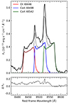 |
Fig. 11. Decomposition of the O Iλ8446 and Ca IIλλ8498, 8542 complex using the Ca IIλ8662 line profile (see Fig. 10) as a template for each line constituting the blended profile (black solid line; upper panel). We are able to reconstruct the O Iλ8446 and Ca IIλλ8498, 8542 complex using a Ca II triplet ratio of 1:1:1 and an O Iλ8446-to-Ca IIλ8662 ratio of 0.85:1. In order to be able to cleanly reconstruct the slope of the blue wing of O Iλ8446, we have to convolve the Ca IIλ8662 template with a Gaussian with a width corresponding to σ = 70 km s−1. The difference between original blended line profile (black solid line) and reconstructed line profile (black dashed line) is shown in the lower panel. |
The reconstruction using three overlapping Ca IIλ8662 profiles cleanly reproduces the key features of the blend of O Iλ8446 and Ca IIλλ8498, 8542. In particular, the two peaks in the blended profile can now be clearly attributed to the overlap of O Iλ8446 and Ca IIλ8498, and of Ca IIλ8498 and Ca IIλ8542. Only one larger residuum remains in the overlap between the red and blue wing of Ca IIλ8498 and Ca IIλ8542, respectively. The underlying emission of ∼0.1 × 10⁻¹⁵ ergs s−1 cm−2 Å−1 is on the level of the left continuum after subtraction of the linear pseudo-continuum. We therefore attribute the difference between the reconstructed blended profile and the observed profile to underlying, additional emission not connected to the O Iλ8446 and Ca IIλ8498, 8542 complex.
3.3. Reconstructing the Balmer line profiles using the Ca II λ8662 difference profile
We demonstrate in Sect. 3.2.3 that the blended line profile of O Iλ8446 and the Ca IIλλ8498, 8542 lines can be decomposed into three individual double-peaked profiles closely resembling that of Ca IIλ8662. While the O Iλ8446 profile and the Ca IIλλ8498, 8542, 8662 profiles are clearly double-peaked, the Balmer lines lines show no clear indication of double peaks. Instead, the presented rms profiles of Hβ and Hα indicate single-peaked emission line profiles, but with a similar redward asymmetry as observed in the Ca IIλ8662 difference profile. In the Hβ and Hα rms profiles, the red wing is ∼400 km s−1 broader (with respect to the central wavelength), while the red wing in the Ca IIλ8662 difference profile is ∼300 km s−1 broader than the blue wing.
We now show that the Balmer line profiles can be reconstructed from the Ca IIλ8662 profile by applying a simple broadening function. To this end, we use a three-parameter Lorentzian
![Mathematical equation: $$ \begin{aligned} I(\lambda ) = I_0 \left[\frac{\Gamma ^2}{(\lambda -\lambda _0)^2 + \Gamma ^2}\right], \end{aligned} $$](/articles/aa/full_html/2024/06/aa48559-23/aa48559-23-eq31.gif) (5)
(5)
where Γ is the half width at half-maximum.
This procedure is motivated by the findings of Kollatschny & Zetzl (2011), who were able to model turbulent motions in the BLR using Lorentzian line profiles, and of Goad et al. (2012), who found that in their bowl-shaped BLR model, Lorentzian line profiles emerge in low-inclination systems for lines formed at larger BLR radii and in the presence of scale-height-dependent turbulence. Therefore, according to the aforementioned models, the broadening by a Lorentzian function in our approach mimics the effects of turbulence in the BLR gas. In addition, other studies also found that emission line profiles in AGN exhibiting line widths of FWHM ≲ 4000 km s−1 are well approximated by Lorentzian profiles (e.g., Véron-Cetty et al. 2001; Sulentic et al. 2002).
For this procedure, we use the Hβ line profile from Spectrum 1 (2015 September 24) as well as the Hβ and Hα rms profiles. For each of these profiles, we broaden the Ca IIλ8662 profile by choosing an appropriate half width Γ such that the broadened Ca II profile matches the corresponding Balmer line profile. In addition, we introduce a velocity shift Δv in order to account for additional blueshifts and redshifts, respectively, of the Balmer lines. The resulting fits and the residual fluxes are shown in Fig. 12. The Hβ line profile from 2015 September 24 is very well approximated by a Ca IIλ8662 line profile that is shifted by Δv = +360 km s−1 and broadened with a Lorentzian with a half width of Γ = 450 km s−1. The only major residuum is a small narrow Hβ component. The Hβ rms profile is also well approximated by applying Lorentzian broadening of half width Γ = 450 km s−1, but this time with a shift of Δv = −50 km s−1. In addition to He IIλ4686, which is already clearly visible in the rms spectrum, we detect emission features at ∼4812 Å, ∼4922 Å and ∼5016 Å in the residual flux in Fig. 12. Based on the resemblance between the emission features at ∼4922, 5016 Å and the difference line profile of He Iλ7065 (see Fig. 9), we identify these emission lines as He Iλλ4922, 5016. The profiles of He Iλλ4922, 5016, 7065 as well as of the unidentified emission feature at ∼4812 are analyzed in more detail in Sect. 3.4. The central Hα rms profile is again well approximated by applying Lorentzian broadening of half width Γ = 450 km s−1 with a shift of Δv = −60 km s−1. However, the line wings are less well approximated and residuals between −2500 km s−1 and +2500 km s−1 are clearly visible in the residual flux. In contrast to Hβ, the residual flux in Hα indicates an additional and very broad component with a full width at zero intensity (FWZI) of FWZI ∼ 20 000 km s−1. This is in agreement with the results of Alloin et al. (1986), who found that the broad Hα line in NGC 1566 line consisted of two components, namely a broad component with an intermediate width of FWHM = 1910 km s−1 and a much broader component with a width of FWHM = 6200 km s−1.
 |
Fig. 12. Reconstruction of the Hβ and Hα line profiles using the Ca IIλ8662 line profile, appropriately shifted by a velocity difference Δv and broadened with a Lorentzian function of half width Γ. The resulting smoothed profiles are shown by a dashed red line (top panels). The residual fluxes are shown in the lower panels. The residual flux of the Hβ profile from Spectrum 1 (2015 September 24) reveals a small residuum from narrow Hβ emission (lower left panel). The residual flux of the reconstructed Hβ rms profile reveals underlying He Iλ4922 emission and possible emission from an unidentified line species at 4812 Å (lower middle panel). While the central rms profile of Hα rms is well approximated by a shifted and broadened Ca IIλ8662 difference profile, we see indications for an additional underlying and extremely broad component in the residual flux (lower right panel). |
3.4. Helium line profiles
We show the rms profiles of He Iλ5016 as well as of the unidentified emission at 4812 Å, and the difference line profile of He Iλ7065 in Fig. 13. In each case, we subtracted a suitable linear pseudo-continuum. All three emission lines have an identical width of FWHM ≈ 2170 km s−1 and show indications of a double-peak structure with the red peak again being stronger than the blue peak. The peaks are positioned at −615 km s−1 and +950 km s−1, and are therefore identical to the peak positions in Ca IIλ8662 (see Sect. 3.2.1). In addition, we again observe a redward asymmetry with the red wing being broader by ∼400 km s−1 with respect to the central velocity.
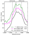 |
Fig. 13. Comparison of the profiles of He Iλ5016, He Iλ7065 and the unidentified line species at approximately 4812 Å in velocity space. We subtracted a suitable linear pseudo-continuum from each line and shifted the profiles in flux for clarity. The positions of the left and right peak of Ca IIλ8662 at −615 km s−1 and +950 km s−1, respectively, are indicated with gray lines. All three line profiles show indications for a similar double-peaked structure and have an identical width of FWHM ≈ 2170 km s−1 when normalized to the profile peak, and of FWHM ≈ 2500 km s−1 when the additional central emission is taken into account. |
In contrast to Ca IIλ8662 (see Fig. 10), the three profiles (see Fig. 13) do not exhibit a central and skewed dip, but instead show additional emission in the region −450 km s−1 < v < +550 km s−1. Supposing that this additional component is superimposed on a double-peaked profile similar to that of Ca IIλ8662, the FWHM of the genuine double-peaked He Iλλ5016, 7065 without the additional component can be estimated to be closer to FWHM ∼ 2500 km s−1.
3.5. The H II region close to the nucleus
An H II region at a separation of only  (corresponding to ∼100 pc) from the nucleus of NGC 1566 was detected by Smajić et al. (2015) and da Silva et al. (2017). Due to the close proximity to the nucleus, we investigate the possible extent of contamination from this region in the nuclear spectra. For this purpose, we extract the spectrum of the H II region from the MUSE data cubes from 2015 September 24 and 2017 October 23, respectively, using a circular aperture of
  . Due to the favorable seeing conditions on 2017 October 23 and the spectrum being taken in AO wide field mode, we scale the spectrum from 2015 September 24 to the integrated [O III] λ5007 flux of (4.2 ± 0.3)×10−15 ergs s−1 cm−2 from 2017 October 23. The spectra are shown in Fig. 14 together with the resulting difference spectrum. Both spectra are dominated by narrow line emission of Hβλ4861, [O III] λλ4959, 5007, [N II] λλ6548, 6583, Hαλ6563, [S II] λλ6716, 6731, [S III] λ9069, absorption of the Ca II triplet, and a strong underlying stellar contribution. For the low-state spectrum from 2015 September 24, the V-band flux amounts to ∼0.3 × 10⁻¹⁵ergs s−1 cm−2 Å−1. The spectra reveal an apparent increase in flux from 2015 September 24 to 2017 October 23, both in the most prominent narrow lines except for [O III] λλ4959, 5007 as well as in the underlying continuum emission. We attribute this to narrow-line flux losses in the extended narrow-line region (NLR) due to unfavorable seeing conditions on 2015 September 24 on the one hand, and scattered radiation from the brightening nucleus on 2017 October 23 on the other hand. The effect of the stray emission from the brightening nucleus is best seen in the Hβ line, where a small broad component appears to emerge on 2017 October 23.
 |
Fig. 14. Spectrum of the H II region at a distance of |

4. Discussion
4.1. Influence of the H II region on the AGN spectra
Stray emission from the H II region at a distance of  from the nucleus can in principle effect the observed AGN spectra by contributing additional continuum and line flux, thereby also effecting the intercalibration of the AGN spectra on the basis of the [O III] λ5007 line. In order to assess the potential effect of stray emission, we inspect the MUSE H II region spectra from 2015 September 24 and 2017 October 24 in Sect. 3.5 and determine an integrated [O III] λ5007 flux of (4.2 ± 0.3)×10−15 ergs s−1 cm−2. This is 4% of the integrated [O III] λ5007 of the nuclear region. However, since the extraction apertures for the nuclear region and the H II region in the MUSE spectra were chosen such that the overlap between the apertures is minimal (see Sect. 2.2), the real contribution from additional [O III] λ5007 from the H II region can be securely estimated to be < 1%, even when taking into account seeing effects. For the SALT spectra, the square aperture of
  for the nuclear region slightly increases the contribution from the H II region, and modest inaccuracies in the exact slit pointing might add to this effect. Nevertheless, the additional contribution in [O III] λ5007 flux can conservatively be estimated to be < 2%.
From the MUSE spectra of the nuclear region and the H II region taken on 2015 September 24, we find that the V-band flux in the H II region is 7% of that in the low-state nuclear spectrum. However, this measurement still includes the strong stellar host-contribution, which we estimate to account for ∼70% of the V-band flux (see Sect. 3.1.1). This reduces the potential continuum contribution of the H II region to the host-free nuclear spectra to ∼4%. Taking into account the minimal overlap between apertures, this further reduces the contribution to < 1% for the MUSE and < 2% for the SALT spectra. We conclude that the H II region contributes only insignificantly to the nuclear spectra presented in this paper.
4.2. The double-peaked Ca II triplet and O I line profiles
4.2.1. Robustness of the double-peaked difference profiles
We show in Sect. 3.2.1 that the difference line profile of Ca IIλ8662 is “lopsided” and double-peaked, exhibiting a skewed dip in the central profile. It closely resembles line profiles observed in a number of AGN and TDEs (see Sect. 3.2.1), which are interpreted to arise in an elliptical accretion disk. To our knowledge, this is the first time “genuine” double-peaked Ca II triplet emission – as well as double-peaked Lβ-pumped O Iλ8446 emission – in AGN has been presented in the literature. Only recently, Dias dos Santos et al. (2023) found, for the first time, a double-peaked O Iλ11279 profile in III Zw 002. Out of the 14 Ca II emitters shown by Persson (1988a), none shows unambiguous indications for a double-peaked profile caused by gas kinematics. Instead, Persson (1988a) attributes the central dips present in some Ca II emitters, such as Mrk 42, to underlying stellar absorption from the host galaxy. However, genuine double-peaked Ca II profiles were detected in spectra of cataclysmic variables and associated with emission from an accretion disk (e.g., Persson 1988b, and references therein).
We omit the effect of Ca II absorption by extracting the Ca II difference line profile between the observations taken on 2015 September 24 and 2017 October 23, respectively. The robustness of the double-peaked profile therefore depends directly on the quality of the intercalibration of these two spectra. The quality of the intercalibration can be directly assessed from Fig. 9. The two spectra we intercalibrated such that the stellar signature of the host galaxy and the narrow lines in the difference profile vanish. The difference spectrum reveals only broad line emission, indicating a successful intercalibration of the two spectra.
The strongest argument for a successful correction for Ca II absorption is provided by comparing the line profile of Ca IIλ8662 with that of O Iλ8446 and Ca IIλ8542. The blue wing of O Iλ8446 is neither influenced by strong absorption nor by blending with Ca IIλ8498. Likewise, the red wing of Ca IIλ8542 is free of absorption as well as line blending effects. We show a comparison of the Ca IIλ8662 difference line profile with the blue wing of O Iλ8446 and the right wing of Ca IIλ8542 in Fig. 15. The profiles of O Iλ8446 and Ca IIλ8542 are normalized to their left and right peak, respectively, and shifted downwards for clarity. All profiles exhibit identical line features, namely a pronounced left peak ➀, the same lopsidedness and characteristic small-scale features in the central profile ➁, and a triple-peaked red peak ➂ that resembles a trident. Although the exact position, width and scaling of the blue peak and the small-scale features in the O Iλ8446 profile differ slightly from that in the Ca IIλ8662 profile, the qualitative profile is identical. We therefore conclude that the Ca IIλ8662 difference line profile presented in Fig. 10 is in fact the clean profile and that residual Ca II absorption is not significantly affecting the line profile. More precisely, the skewed, lopsided profile is exclusively due to the structure and kinematics of the BLR.
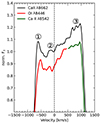 |
Fig. 15. Comparison of the Ca IIλ8662 difference line profile (black) with the blue wing of O Iλ8446 (red) and the right wing of Ca IIλ8542 (green) in velocity space. The profiles of O Iλ8446 (red) and Ca IIλ8542 are normalized to their left and right peak, respectively, and shifted downwards for clarity. All profiles exhibit identical line features, namely a pronounced left peak ➀, the same lopsidedness and characteristic small-scale features in the central profile ➁, and a triple-peaked (trident) red peak ➂. |
4.2.2. The elliptical accretion disk model for Ca II λ8662
We show in Sect. 3.2.2 that the Ca IIλ8662 difference profile (and in turn the O I profile and the other Ca II profiles), with exception of the inner part of the profile, is in general well approximated by line emission from a relativistic elliptical accretion disk. In particular, the model reproduces the observed shape of the line wings, and only the red peak of the model fit is marginally shifted inwards by about 50 km s−1 with respect to the observed profile. This indicates that the structure (and/or kinematics) of the disk generating the line profile might be more complex than a homogeneous elliptical disk, thereby causing the trident structure in the red peak (see Sect. 4.4.3 for further details).
The model reproduces a low disk inclination of i = (8.10 ± 3.00)° in agreement with findings of Parker et al. (2019), who found i < 11°, and with the almost face-on view of the host galaxy, though we note that NGC 1566’s host-galaxy geometry is more complex on larger scales (Elagali et al. 2019). The major axis viewing angle, which is the angle between the major axis in apocenter direction and the projected line-of-sight in the disk plane, is ϕ0 = (193.29 ± 26.00)°. The disk is confined within the inner and outer pericenter distances ξ1 and ξ2 of (2231 ± 1000) rg and (4050 ± 1500) rg, respectively, and exhibits very low internal broadening with σ = (87 ± 10) km s−1. The eccentricity of e = 0.57 ± 0.35 is moderate, and the emissivity power-law index q amounts to 4.34 ± 0.80. This is larger than the value of q ≈ 3 for the emissivity profile of an outer accretion disk (≳100 rg) irradiated by an isotropic point source (or simple extended source) of X-ray emission (see Wilkins & Fabian 2012, and references therein) usually adopted in other studies (e.g., Eracleous & Halpern 1994, 2003).
Our best-fit model is able to reproduce all key features of the Ca IIλ8662 profile, namely the redward asymmetry and the narrow blue and red peak, respectively. It cannot, however, account for all of the emission in the central part of the profile between −450 km s−1 < v < +850 km s−1. This discrepancy between disk-modeled line profiles and observed line profiles has been noticed in other studies (e.g., Hung et al. 2020; Wevers et al. 2022; Dias dos Santos et al. 2023), and has been attributed to additional emission from gas above the disk plane. In contrast to previous studies, we do not attempt to recover the additional emission component by a Gaussian component as this component in our model is clearly not a Gaussian. Instead, the central emission component has a distorted, rather flat-topped profile with a pronounced redward asymmetry.
In agreement with the aforementioned studies, we attribute this additional emission component to emission from BLR clouds situated above the accretion disk plane, apparently not retaining the angular momentum of the disk. The observed redward asymmetry might be explained by the asymmetric distribution of clouds with respect to the ionizing continuum, which we assume to be in close vicinity to the SMBH. Regardless of the exact distribution of BLR gas above the disk, we conclude that the BLR in NGC 1566 is a two-component BLR, consisting of a BLR disk component and an additional component of BLR gas above the disk plane.
For a sample of six AGN, Eracleous et al. (1995) found pericenter distances ξ1 and ξ2 for Hα ranging between 350 − 1900 rg and 3000 − 9000 rg, respectively. For a sample of 116 double-peaked Balmer line AGN, Strateva et al. (2003) found the accretion disks to be consistent with inner radii of (200 − 800) rg, and outer radii ≥2000 rg. This places our inner pericenter distance ξ1 at the higher end of the distribution, and the outer pericenter distance ξ2 at the lower end. Nevertheless, the scatter in the modeled disk extents for different objects is rather large. For example, Ricci & Steiner (2019) found both pericenter distances ξ1 and ξ2 for Hα in NGC 4958 to be < 1000 rg. Storchi-Bergmann et al. (1997) found pericenter distances ξ1 and ξ2 of 1300 rg and 1600 rg in NGC 1097 using their refined elliptical disk model, indicating a rather ring-like structure.
In order to test the robustness of our solution, we now calculate the expected lag of Hβ using the RHβ − λL5100 relationship
![Mathematical equation: $$ \begin{aligned} \mathrm{log}\left[\frac{R}{\mathrm{1\,lt\text{-}day}}\right] = K + \beta \, {\log }\left[\frac{\lambda L_{5100}}{10^{44}\,\mathrm{erg\,s}^{-1}}\right], \end{aligned} $$](/articles/aa/full_html/2024/06/aa48559-23/aa48559-23-eq37.gif) (6)
(6)
where K is the origin and β is the slope of the relation. We expect Hβ to be emitted at approximately the same radial distance as Ca IIλ8662, since we can model the Hβ profile as a Ca IIλ8662 profile broadened by a Lorentzian function. This is interpreted as the effect of scale-height-dependent turbulence (see Sect. 4.4.1), which in turn means that the underlying rotational kinematics of Hβ and Ca II are identical. Recent works suggest that the FWHM of Hβ and Ca II in high-luminosity sources are tightly correlated, while the FWHM of Hβ in local low-luminosity sources like NGC 1566 is slightly larger than that of Ca II (Martínez-Aldama et al. 2021). We use a slope of β = 0.53 as found by Bentz et al. (2013) and Kollatschny et al. (2018), K = 1.53, and adopt λL5100 = 3.91 × 1041 ergs s−1 obtained in Sect. 3.1.3. This gives a BLR radius of only ∼1.8 lt-days. We now compare this value with the delay expected from the best-fit elliptical accretion disk model calculated in Sect. 3.2.2. For this purpose, we first calculate the distance d = ξ2/(1 − e)−ξ2 of the center of the disk to the SMBH using the outer perigee ξ2 of the disk emitting region and the eccentricity e. This gives a distance of d ≈ 5500 rg from the SMBH to the disk center, and with MBH = (5.3 ± 2.7)×106 M⊙ calculated in Sect. 3.1.3, which results in a gravitational radius rg = GM/c2 of 0.0003 lt-days, we obtain ∼1.7 lt-days for the expected delay between continuum and line emission in NGC 1566. This is a rough estimate, since the line emission is not weighted by emissivity. Nonetheless, this simple order-of-magnitude assessment confirms that the best-fit disk parameters are in good agreement with established reverberation mapping scaling relations.
4.2.3. The Bowen fluorescence line O I λ8446 as part of the elliptical disk model
We find indications for O Iλ8446 as well as Ca II triplet emission already being present during the low-state, host-galaxy subtracted spectrum from 2015 September 24 (Spectrum 1; see Fig. 4). Although the S/N of O I and Ca II in the host-galaxy subtracted spectrum is low and the Ca II triplet is still affected by residual absorption, we identify the blue wing of O Iλ8446 together with its blue peak. We show a comparison between the blue O Iλ8446 wing from 2015 September 24 and the blue O Iλ8446 wing from the difference spectrum in Fig. 16. The blue wing of O Iλ8446 from the low-state spectrum is scaled and smoothed for clarity. We find a blueward drift of about −(150 − 200) km s−1 with respect to the low-state spectrum. For comparison, Hβ shifted by −240 km s−1 between Spectrum 1 and Spectrum 2 (from 2015 September 24 to 2017 October 23). This indicates that O Iλ8446 shifts in tandem with the Balmer lines (see Sect. 3.1.2), but not necessarily by the exact same amount8.
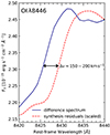 |
Fig. 16. Comparison of the blue wing of O Iλ8446 between the difference spectrum from 2015 September 24 to 2017 October 23 (blue) and the host-subtracted residuum spectrum from 2015 September 24 (slightly smoothed and scaled for clarity; red) resulting from the stellar synthesis in Sect. 3.1.1. The shift of the blue wing of O Iλ8446 from 2015 September 24 to 2017 October 23 indicates a blueward drift of the line emission. The difference velocity Δvshift amounts to Δvshift ≈ 150 − 200 km s−1. |
In the following, we discuss the production channels of O Iλ8446 and its region of origin. O Iλ8446 emission can be produced by either recombination, collisional excitation by electrons, continuum fluorescence, Lyβ fluorescence (a process first described by Bowen 1947, hence also termed Bowen fluorescence) or a combination of these mechanisms (for a review see Grandi 1980). The exact mechanism(s) responsible for the emission of O Iλ8446 in a particular source can be determined by performing line diagnostics with respect to other O I lines in this source. Rodríguez-Ardila et al. (2002a) performed line diagnostics on the O I lines λλ1304, 7774, 8446, 11287 in a sample of six AGN. They found O Iλ8446 to be formed through collisional excitation and Lyβ fluorescence, and excluded recombination and continuum fluorescence as a source of the observed line strength of O Iλ8446. Matsuoka et al. (2007) later corroborated these results by means of photoionization models.
O Iλ8446 emission in AGN has been known for several decades, and has early been associated with the broad line region due to the absence of a narrow component (Grandi 1980). We can confirm the absence of a narrow O Iλ8446 component in NGC 1566, and, moreover, report that O Iλ8446 and the lines of the NIR Ca II triplet exhibit virtually identical line profiles (see Fig. 15). Persson (1988a) found a tight correlation between the FWHM of O Iλ8446 and the Ca II triplet, indicating that the O I and Ca II lines stem from approximately the same region. Likewise, Rodríguez-Ardila et al. (2002b) concluded by virtue of identical line profiles, that O I and Ca II share the same kinematics. We can confirm this result based on the identical line profiles, that place the emitting gas in a region dominated by the kinematics of an elliptical disk (see Sect. 4.2.2). We stress, however, that the profile of O Iλ8446 exhibits a more redshifted blue peak and a shallower blue wing than Ca IIλ8662. This required convolving the Ca IIλ8662 profile with a Gaussian of small width in order to reproduce the slope of the left wing of O Iλ8446 when reconstructing the blended O I and Ca II triplet complex. Such a slight change in the profile’s shape can be achieved in the best-fit Ca IIλ8662 model by increasing the inner pericenter distance ξ1 by about 10%. We therefore speculate that emission of O Iλ8446 takes place in a similar, overlapping region with respect to emission of Ca II, and that this region has a marginally larger inner radius.
Bowen fluorescence lines have recently gained attention by the detection and definition of a new class of transient events in AGN by Trakhtenbrot et al. (2019b). They described a new class of long-lived (a few years) transient events during which broad N IIIλ4640 (as well as O IIIλ3133 and N IIIλλ4097, 4103; see Makrygianni et al. 2023, and references therein) is generated by the absorption of He II Lyα by O III. O III then de-excites through a series of optical transitions and a far-UV transition at 374.436 Å, which in turn excites N III, generating optical emission of N IIIλλ4097, 4104, 4379, 4634, 4641 (Bowen 1928, 1935). We note that Lβ pumping, and therefore the generation of O Iλ8446, follows a different production channel, namely the absorption of H I Lβ (1025.72 Å) by O I, directly leading to the emission of O Iλλ1304, 8446, 11287 through optical de-excitation.
The presence of enhanced ionizing UV emission during Bowen fluorescence flares has been attributed to enhanced accretion onto the SMBH (Trakhtenbrot et al. 2019b; Makrygianni et al. 2023) in a pre-existing AGN. Based on the detection of weak O Iλ8446 emission in NGC 1566 present already before the transient event, we likewise attribute the enhanced UV emission (Oknyansky et al. 2020) and the in turn enhanced O Iλ8446 emission during the event to an increase in accretion rate.
4.2.4. Density and column density in the O I and Ca II disk
Based on the almost identical line profiles of O Iλ8446 and Ca II, we show in Sect. 4.2.3 that both lines originate from approximately the same region, and that this region is dominated by the kinematics of an elliptical accretion disk. We now show that this is consistent with photoionization calculations, which indicate that both O Iλ8446 and Ca II are emitted from a region of similar (column) density. In Sect. 3.2.3, we find a Ca II triplet ratio of 1:1:1 and an O Iλ8446-to-Ca IIλ8662 ratio of 0.85:1. The Ca II T: O Iλ8446 ratio is therefore 3.5. Persson (1988a) pointed out that if Ca II triplet emission is detected in AGN, the Ca II triplet ratio is usually on the order of 1:1:1. This indicates that the Ca II emission arises from a region that is optically thick in Ca II. Model calculations for Ca II (Joly 1989; Ferland & Persson 1989) placed the emitting region in a cool and dense gas with a temperature T ≤ 8000 K, a density of nH ≃ 1012 cm−3, and a column density of NH ≥ 1023 cm−2. More recent studies corroborated the results for the gas and column density (Panda et al. 2020; Panda 2021a,b). These physical conditions are the conditions of an outer, cold accretion disk, and Ferland & Persson (1989) and later Dultzin-Hacyan et al. (1999) associated Ca II emission with a wind (or corona) just above the accretion disk. Based on photoionization model calculations on surveys of intermediate-redshift quasars, Matsuoka et al. (2007) and Martínez-Aldama et al. (2015) suggested that O Iλ8446 and the Ca II triplet are emitted from regions with similar physical conditions. In particular, Matsuoka et al. (2007) restricted the density of the O I and Ca II emitting gas to nH ≃ 1011.5 cm−3, and based on our measured Ca II T: O Iλ8446 ratio of 3.5 in NGC 1566, their model gives a column density of NH ≃ 1.2 × 1023 cm−2 (see Fig. 8 in Matsuoka et al. 2007) for the O Iλ8446 emitting region in NGC 1566. In summary, we suggest that O I and Ca II are emitted in a similar, overlapping region, as argued before on basis of the identical line profiles.
4.3. Helium profiles and the unidentified emission at 4812 Å
In Sects. 3.3 and 3.4 we identify emission of He Iλλ4922, 5016, 7065 based on their identical line profiles. The profiles of He Iλλ5016, 7065 show, in comparison to the profiles of O Iλ8446, Ca IIλλ8498, 8542, 8662, and the “smoothed” profile of Hβ, a much stronger central emission component, whereas the double-peak structure is almost completely suppressed. The He I profiles bear a remarkable resemblance to the late-time Hα profiles observed in the TDE AT 2018hyz by Hung et al. (2020), when the central additional emission starts to dominate the line profile. Hung et al. (2020) identified the additional emission to be a nondisk Gaussian component related to a BLR that formed by radiatively driven winds. Likewise, the BLR in NGC 1566 can be modeled as a two-component BLR, namely BLR disk and BLR gas above the disk plane, where the BLR component from above the disk contributes more to the He I lines than to the other line species. At the same time, the FWHM of the He I disk-component in NGC 1566 is ∼2500 km s−1 and therefore broader by ∼600 km s−1 and ∼300 km s−1 in comparison to Ca IIλ8662 and Hβ, respectively.
The detection of the yet unidentified emission at ∼4812 Å is based on the striking resemblance between this emission line and the He Iλλ5016, 7065 profiles, all of them exhibiting approximately the same width, weak double-peak features and additional strong emission in the central line profile with almost identical small-scale features. The pronounced similarity between the profiles might suggest that this is genuine emission and not just a residual from the reconstruction of Hβ from the double-peaked Ca II profile. If indeed line emission, the exact identification of the line species is difficult, since the central wavelength of ∼4812 Å is estimated by comparing the line profile with that of He Iλλ5016, 7065. As shown previously, Hβ and O Iλ8446 show significant, but not necessarily identical blueward drifts during the rising phase of the transient event, and we suspect the same to be true for all broad lines. Consequently, we cannot exactly determine the central wavelength of the unidentified emission. Despite the resemblance to the He I profiles, we find the emission at ∼4812 Å unlikely to be associated with He I as no emission from He I is expected in a spectral range ±100 Å around this wavelength (see the NIST Atomic Spectra Database9).
Véron et al. (2002) associated the “red shelf” observed in some Seyfert 1s (Meyers & Peterson 1985) with broad emission from He Iλ4922 and He Iλ5016. We confirm the presence of He Iλλ4922, 5016 in NGC 1566 and that they constitute the red shelf of Hβ clearly discernible in the rms spectrum close to Hβ (see Fig. 12). Although the blue wing of He Iλ4922 is slightly disturbed by either interference from small Hβ residuals or unidentified line emission, the red wing shows the same shape as the other He I lines. We also find indications for the red wing of He Iλ4713, however, this line is heavily blended with He IIλ4686. The spectral region between ∼4500 Å and ∼5600 Å in AGN can be densely populated by line emission of Fe II, and previous studies found tight correlations between the properties of Ca II and Fe II emitting regions (Panda et al. 2020; Panda 2021a,b). In particular, Ca II and Fe II are expected to be emitted from gas with the same temperature, density, column density, and their line profile widths indicate an origin from approximately the same spatial region (Marinello et al. 2016, 2020). Hence, since NGC 1566 shows strong Ca II emission, significant optical Fe II emission is expected. Indeed, we observe strong line emission between ∼4500 Å and ∼5600 Å during the transient event, requiring a careful decomposition and fitting in order to determine the different line contributions. This is, however, beyond the scope of this paper.
4.4. Broad-line region structure and kinematics
4.4.1. The role of turbulence and stratification in the BLR
Spectrum 1 (2015 September 24) and Spectrum 2 (2017 October 23) exhibit very similar Hβ line profiles, and we show in Sect. 3.3 that the low-state Hβ profile is in perfect agreement with a double-peaked Ca IIλ8662 profile smoothed by a Lorentzian of half width Γ = 450 km s−1. The resulting profile itself is not a Lorentzian profile, but is asymmetrical and slightly skewed due to the underlying double-peaked profile. Likewise, we can model the rms profiles of Hβ and Hα by exactly the same procedure10. This indicates that underlying kinematics do not change drastically during the transient event. We draw two major conclusions from these results: First, since the low-state Hβ profile before the transient event is evidently shaped by the same elliptical-disk kinematics as Ca IIλ8662, the disk-like BLR was already present before the transient event began in 2017. Second, the Hβ profile is influenced by some physical process effectively smearing out the profile with respect to the double-peaked Ca IIλ profile. In the following, we show that this smearing of the profile can be attributed to turbulence.
Kollatschny & Zetzl (2013a,b) were able to parameterize broad emission lines in AGN by the ratio of FWHM to line dispersion σline, and modeled line profiles shaped by scale-height-dependent turbulence as Lorentzian profiles. They obtained distances R of the line emitting region using reverberation mapping and modeled the scale height H according to
 (7)
(7)
given by Pringle (1981), where α is the viscosity parameter of order unity. The velocities give the turbulent and rotational velocities, respectively. Kollatschny & Zetzl (2013a,b) found a flattened distribution for the Hβ emitting region, and in particular that the height of the line emitting region increases with distance to the SMBH, resulting in a flat bowl-shaped geometry. Strikingly, Kollatschny & Zetzl (2013a) found for a large sample of AGN that each emission line was associated with a specific turbulent velocity, and in particular that the turbulent component in Hβ profiles corresponded to turbulent motions of vturb ∼ 400 km s−1. Goad et al. (2012) found that Lorentzian profiles of the emission lines naturally arise for low-inclination systems in their bowl-shaped BLR model, and evidence for bowl-shaped BLR geometries (e.g., Ramolla et al. 2018, and references therein) or in general flattened or disk-like geometries (e.g., Gaskell et al. 2007; Pancoast et al. 2014; Williams et al. 2018) have also been found by other studies.
As the temporal sampling of the presented variability campaign of NGC 1566 during the transient event is too low to perform classical reverberation mapping, we are not able to obtain geometrical information from the transfer function. Therefore, we cannot make a precise prediction about the exact shape of the BLR; that is, whether it is rather disk-like or bowl-shaped. However, as the aforementioned models associate turbulence with scale height above the disk, we deduce a vertical stratification of the BLR; that is, Hβ is emitted at greater scale height than Ca II and O I: For α set to 1, the turbulent velocities v(CaII)turb = 200 km s−1 (see Sect. 4.2.2) and v(Hβ)turb = 900 km s−1 as well as FWHM (Ca II) = 1920 km s−1 and FWHM (Hβ) = 2200 km s−1, we obtain an H/R value of ∼0.1 and ∼0.4 for Ca II and Hβ, respectively. Therefore, Hβ is being emitted roughly at four times the height of Ca II.
Although the He I profiles do not allow for a reliable fit with the elliptical disk model alone, we note that we can in principle construct such “smeared out” broader profiles (in comparison to Hβ) by decreasing the inner and outer pericenter distance of the emitting region while at the same time increasing the internal broadening. This indicates that the He I emission is generated at shorter distances from the ionizing continuum (“further in”), paired with higher internal broadening, which can be interpreted as turbulence due to greater scale height and therefore a higher layer in the disk. This is in agreement with results of Kollatschny & Zetzl (2013b), who showed that high-ionization lines are emitted closer to the SMBH, but at greater heights.
In conclusion, we term the BLR in NGC 1566 to be disk-dominated. This means that all broad emission lines analyzed in this study (Hβ, He I, Ca II, and O I) show the kinematic signature of an elliptical accretion disk. While this signature is clearly visible in the line profiles of Ca II, and O I as they are being emitted closest to the midplane of the disk, it is smeared out by turbulence (and in some part by the presence of additional emission components) in the case of Hβ and He I.
4.4.2. Temporal evolution of the Balmer profiles: A possible disk wind
We show in Sects. 3.1.2 and 4.2.3, that Hβ and O Iλ8446 exhibit blueward drifts by −240 km s−1 and −(150 − 200) km s−1, respectively, during the rising phase of the transient event (between Spectrum 1 and Spectrum 2). When fitting line profiles with accretion disk models, velocity shifts due to other physical processes affect the (a)symmetry of the profile and may prevent the determination of the true disk parameters if not taken into account. This problem regarding velocity shifted line profiles has already been addressed by Eracleous et al. (1995) and Eracleous & Halpern (2003) with respect to possible orbital motions in a binary system used to explain the formation of eccentric disks. In the following, we investigate the impact of the blueward drift on the best-fit parameter set and discuss possible explanations for the observed line profile shifts.
Supposing that Ca II exhibits a velocity shift similar to O Iλ8446, and that the line profile does not change significantly (as indicated by the almost identical Hβ profiles during the onset of the transient event), we perform a fit on a Ca IIλ8662 profile that we artificially redshift by +200 km s−1. This way, we compensate the blueward drift of the line during the transient event and obtain, presumably, the original Ca IIλ8662 before the transient event. We find that we are able to fit the shifted Ca IIλ8662 profile with the disk parameters ξ1 = (1140 ± 800) rg, ξ2 = (4468 ± 1600) rg, i = (5.64 ± 3.00)°, ϕ0 = (207.94 ± 26.00)°, σ = (85 ± 10) km s−1, e = (0.55 ± 0.40), and q = (4.50 ± 0.90). This fit largely reproduces the best-fit parameters obtained in Sect. 3.2.2 within their error margins, except for the inner pericenter distance ξ1, which decreased by half and is now slightly below the determined margin of error.
We now discuss the blueward drift of the Hβ profile in the context of line profiles presented in previous studies. The Hβ profile shifted by −240 km s−1 within ∼750 days (between Spectrum 1 and Spectrum 2) and by additional −130 km s−1 within the next 270 days (between Spectrum 2 and Spectrum 3; see Fig. 8). However, previous low-state observations over the last 30 years indicate a constant redshift of the Hβ line. Kriss et al. (1991) found an Hβbroad velocity shift of ∼ + 700 km s−1 in their HST/FOS spectrum from 1991. Likewise, we find an Hβ redshift of ( + 670 ± 50) km s−1 in the mean spectrum of a variability campaign on NGC 1566 we performed from 2012 November to 2013 March from which we presented a spectrum in Ochmann et al. (2020). A velocity shift of ( + 375 ± 6) km s−1 in a GMOS spectrum obtained in 2013 October was reported by da Silva et al. (2017). However, their analysis is primarily based on Hα due to its preferable S/N, and the Gaussian fit to Hβbroad does not capture the line profile of Hβ well. As the Hβ profile from da Silva et al. (2017) and the line profile from our 2012 to 2013 campaign are, by visual inspection, virtually identical, we conclude that the velocity shift in the GMOS spectrum from 2013 October is in fact closer to ∼ + 700 km s−1. The stability of the Hβ (and Hα) profile was already pointed out by Alloin et al. (1985), who noticed that no considerable changes in the shape of the broad components were present, despite ample changes in total flux during their observations lasting from 1980 to 1982.
Given the stability of the line profile on timescales of years, the consistent velocity shift of ∼ + 700 km s−1 for Hβbroad over the last 30 years, and indications for slightly different velocity shifts in Hβ and O Iλ8446, a disk wind might serve as an intuitive explanation for the observed blueward drift of the Hβ profile. Accretion disk winds are thought to play an important role in the formation of the BLR (Czerny & Hryniewicz 2011), and they have been invoked to explain several observational key features of the BLR, for example, the lower redshifts of low-ionization broad emission lines (BELs) in comparison to high-ionization BELs (Gaskell 1982), or the broad absorption lines (BALs) seen in the UV spectra of some AGN (Weymann et al. 1991). Gaskell (1982) tied the different redshifts between low- and high-ionization BELs to two different ionization zones, and it was later suggested that these zones are the low-ionization surface layer of a high-density accretion disk and a high-ionization, low-density wind launched from the accretion disk (Collin-Souffrin 1987; Collin-Souffrin et al. 1988, and references therein). Generally, accretion disk winds can have a severe impact on the observed line profile shapes, in particular depending on the optical depth of the wind (e.g., Chiang & Murray 1996; Murray & Chiang 1997; Flohic et al. 2012). If the optical depth is low, accretion disk winds can induce blueshifts on lines without changing their profiles (Eracleous & Halpern 2003). A disk wind would be consistent with results from Parker et al. (2019), who found indications for a v ∼ 500 km s−1 outflow being launched during the outburst in NGC 1566. On basis of the results presented in this paper, namely the blueward drift of the line profiles and differing velocity shifts between individual lines, we propose a launching accretion disk wind as an explanation for the blueward drift of Hβ and O Iλ8446 during the rising phase of the transient event in NGC 1566.
We note that changes in the line profiles caused by accretion disk winds might explain the more complex Hβ profiles observed in later stages of the transient event (see Fig. 7), when NGC 1566 transitions from a Sy 1.2 back to a Sy 1.8 galaxy (Elitzur et al. 2014).
4.4.3. Evidence for BLR (and AD) inhomogeneities
We show in Sect. 4.2.1 that the small-scale features in the O I and Ca II line profiles are not caused by absorption or blending effects, but are genuine features of the double-peaked profiles. The homogeneous elliptical disk model applied in Sect. 3.2.2 is not able to account for these features, and the small-scale variations in the profile remain imprinted on the residual flux. The most prominent deviation from the elliptical-disk profile is the trident structure in the red peak, that appears to be constituted by three individual, overlapping peaks. This might, for example, indicate that the inner orbit of the BLR disk in NGC 1566 is in fact split, such that the high-velocity part of the profile splits up. Although our current modeling cannot distinguish if the small-scale line features in the two-component BLR model originate from the disk or the gas above the disk plane, the trident in the red peak makes it intriguing to associate the small-scale deviations with inhomogeneities in the BLR disk structure, which we argue to be tightly connected to an underlying accretion flow. Inhomogeneities appear to be a key feature in AGN accretion disks (e.g., Dexter & Agol 2011; Jiang & Blaes 2020), and are, for example, invoked to explain the variability in AGN. Inhomogeneities in the BLR have been invoked in the literature in the past to explain broad-line profile changes (e.g., Veilleux & Zheng 1991; Wanders 1995) on timescales of years, and more recently Horne et al. (2021) identified azimuthal structures rotating in the BLR of NGC 5548, revealing that the BLR is not a homogeneous entity. Structural BLR models incorporating inhomogeneities in the BLR invoke, among others, spiral arms or hot spots in the disk (e.g., Gilbert et al. 1999; Storchi-Bergmann et al. 2003; Jovanović et al. 2010) and spiral arm models are able to explain the generally observed differences between average and rms profiles as well as complex subfeatures in velocity-delay maps (Wang et al. 2022; Du & Wang 2023). The detection of BLR inhomogeneities in the profiles of O I and Ca II in NGC 1566 suggests that reverberation mapping of these lines could be a powerful instrument to investigate the BLR structure in AGN in more detail. This has already been noted by Matsuoka et al. (2008).
4.4.4. A turbulent and disk-dominated BLR model as an explanation for the observed emission line profiles
We show above that the line profiles in NGC 1566 during the transient event are shaped by the superposition of at least three effects: (1) the asymmetric and double-peaked O I and Ca II profiles can be modeled by an elliptical, eccentric disk component; (2) the Hβ line profiles can be modeled as broadened versions of these profiles, a fact that we ascribe to scale-height-dependent turbulence; and (3) the line profiles exhibit blueward drifts during the rising phase of the transient event, a circumstance that might be interpreted as the signature of a low-optical-depth disk wind being launched during the transient event. In the emerging BLR picture, the BLR is not only radially stratified with regard to its ionization structure, but also vertically stratified with regard to scale-height-dependent turbulence. Based on the larger FWHM of the He I lines in comparison to Hβ, O I, and Ca II, He I is presumably emitted at shorter radial distance from the ionizing source than the other lines. Furthermore, according to our model Hβ is emitted at greater scale height than O I, and Ca II, but roughly at the same radial distance. To illustrate, we show a qualitative sketch of our BLR model in Fig. 17.
 |
Fig. 17. Qualitative edge-on view of the BLR geometry suggested for NGC 1566 (not to scale and the height of the BLR above the disk plane is largely exaggerated for clarity). The blue and red color of the disk vaguely represents the transition from a hotter inner to a cooler outer accretion disk. The BLR has a flattened distribution, with O I and Ca II being emitted close to the midplane of the accretion disk. Hβ is emitted at greater scale height. He I is emitted at shorter radial distance from the ionizing source. |
5. Conclusions
In this study, we present results of a spectroscopic variability campaign performed on NGC 1566 during its transient event from 2017 to 2019. In particular, we analyzed the emission line profiles of Ca II, O I, He I, Hβ, and Hα, and the corresponding profile changes during the event. Our results can be summarized as follows:
-
NGC 1566 exhibits strong spectral changes during its transient event from 2017 to 2019. We observe the emergence and subsequent fading of a strong, power-law-like blue continuum as well as the brightening and subsequent fading of strong Balmer, He I, and He II lines. In addition, we observe variable coronal line emission of [Fe VII], [Fe X], and [Fe XI]. Further, more detailed results on the spectral variability in NGC 1566 during its transient event will be presented in future publications.
-
We report the detection of double-peaked profiles of the Bowen-fluorescence line O Iλ8446 and Ca II with redward asymmetry during the transient event. To our knowledge, this is the first time that genuine double-peaked O Iλ8446 and Ca II triplet emission line profiles in AGN have been presented in the literature. Moreover, we find indications that O Iλ8446 as well as NIR Ca II triplet emission was already present before the onset of the transient event. The O Iλ8446 and Ca II triplet emission line profiles are well approximated by a combination of emission from an eccentric disk with a low inclination angle of i = (8.10 ± 3.00)° and an emission component from BLR gas above the disk. In addition, we interpret small-scale features in the Ca II line profile as evidence for inhomogeneities in the broad-line region associated with the accretion disk.
-
We find a NIR Ca II triplet ratio of 1:1:1 and an O Iλ8446-to-Ca IIλ8662 ratio of 0.85:1. Based on the results of previous studies by other authors, this suggests that the emission of O I and Ca II originates from approximately the same region, namely a region of high (column) density with the kinematic signature of a rotating disk.
-
Based on the stable line profiles and the constant FWHM of Hβ during the event, and Lβ-pumped O Iλ8446 emission already being present before the brightening in NGC 1566, we conclude that the broad-line region associated with the disk was already present before the beginning of the transient event. More specifically, we postulate that the elliptical disk and the associated broad-line region were not formed during the transient event, but were present before the event began.
-
We show that the Balmer line profiles in NGC 1566 exhibit the same redward asymmetry as the O I and Ca II lines, and that, in comparison, they have a slightly larger FWHM. We are able to reconstruct the Hβ and Hα rms profiles by convolving the double-peaked Ca IIλ8662 profile with a Lorentzian with a width of ∼900 km s−1. We suggest that this might be interpreted as broadening due to turbulent motions of the Balmer-line-emitting gas and that this turbulence smears out the double-peaked profile. According to this interpretation, the region of Balmer line emission in the broad-line region is most likely situated at greater scale height above the accretion disk than the region emitting Ca II.
-
We find indications for a blueward drift of the total Hβ and O Iλ8446 profiles during the rising phase of the transient event. These varying velocity shifts might be interpreted as the emergence of a low-optical-depth wind being launched during the transient event. Except for this launching disk wind, the observed kinematics of the BLR remain largely unchanged during the transient event.
Our results suggest a flattened (disk-dominated) broad-line region geometry, with a vertical stratification due to winds in combination with turbulence. Our results demonstrate the usefulness of spectroscopic transient variability campaigns with high data quality, even when sampling is sparse. We especially point out the usefulness of observations of O Iλ8446 and the NIR Ca II triplet, which is due to the close proximity of their emission region to the accretion disk. Further, more densely sampled spectroscopic observations of transient events are strongly desired.
Sy 1 galaxies show Balmer lines that are wider than the forbidden lines, while Sy 2 galaxies show Balmer lines that are about the same width as the forbidden lines (Khachikian & Weedman 1974). The types Sy 1.2, Sy 1.5, Sy 1.8, and Sy 1.9 galaxies are subtypes, with numerically larger Seyfert classes showing weaker broad emission with respect to the narrow lines (Osterbrock 1977, 1981; Winkler 1992).
We note that the narrow component of Hα in Spectrum 2 obtained with MUSE is affected by overexposure, which considerably reduces the measured flux of Hαnarrow.
We also note that when presented the possibility to choose from a range of power laws with different indices, pPXF always prefers the power law with the smallest index.
We also use the reconstructed profile from Sect. 3.3 to determine the redshift of the line.
We also find apparent blueward drifts of the same order in the red wings of Ca IIλ8662 and Ca IIλ8662. However, the S/N in the host-galaxy-subtracted spectrum is too low and the profiles are affected by residual absorption, meaning that no robust quantitative estimate of the shift can be made.
We note that the rms spectrum is dominated by the two strongest spectra closest to the transient peak.
Acknowledgments
The authors thank the anonymous referee for detailed and useful comments, which contributed significantly to the improvement of the manuscript. Furthermore, the authors thank Peter M. Weilbacher for helpful discussions regarding the MUSE reduction pipeline, Dragana Ilić for enlightening discussions about emission lines in optical spectra, Paul I. Schwarz for computational advice as well as helpful discussions, and Björn Müller for discussions regarding mathematical details of the fit to the Ca II profile. The authors greatly acknowledge support by the DFG grants KO 857/35-1 and CH 71/34-3. M.W.O. gratefully acknowledges the support of the German Aerospace Center (DLR) within the framework of the “Verbundforschung Astronomie und Astrophysik” through grant 50OR2305 with funds from the German Federal Ministry for Economic Affairs and Climate Action (BMWK). E.R.C. acknowledges support from the National Research Foundation of South Africa. Five spectra reported in this paper were obtained with the Southern African Large Telescope (SALT under proposal codes 2018-1-DDT-004, 2018-1-DDT-008 (PI: Kollatschny) and 2018-2-LSP-001 (PI: Buckley)). In addition, this paper is based on observations made with ESO Telescopes at the La Silla Paranal Observatory under programme IDs 096.D-0263 and 0100.B-0116, obtained from the ESO Science Archive Facility.
References
- Alloin, D., Pelat, D., Phillips, M., & Whittle, M. 1985, ApJ, 288, 205 [NASA ADS] [CrossRef] [Google Scholar]
- Alloin, D., Pelat, D., Phillips, M. M., Fosbury, R. A. E., & Freeman, K. 1986, ApJ, 308, 23 [NASA ADS] [CrossRef] [Google Scholar]
- Antonucci, R. 1993, ARA&A, 31, 473 [Google Scholar]
- Bacon, R., Accardo, M., Adjali, L., et al. 2010, in Ground-based and Airborne Instrumentation for Astronomy III, eds. I. S. McLean, S. K. Ramsay, & H. Takami (SPIE), Int. Soc. Opt. Photon., 7735, 131 [Google Scholar]
- Bacon, R., Vernet, J., Borisova, E., et al. 2014, The Messenger, 157, 13 [NASA ADS] [Google Scholar]
- Baldwin, J., Ferland, G., Korista, K., & Verner, D. 1995, ApJ, 455, L119 [NASA ADS] [Google Scholar]
- Bentz, M. C., Denney, K. D., Grier, C. J., et al. 2013, ApJ, 767, 149 [Google Scholar]
- Blandford, R. D., & McKee, C. F. 1982, ApJ, 255, 419 [Google Scholar]
- Bon, E., Marziani, P., & Bon, N. 2017, in New Frontiers in Black Hole Astrophysics, ed. A. Gomboc, IAU Symp., 324, 176 [NASA ADS] [Google Scholar]
- Bowen, I. S. 1928, ApJ, 67, 1 [Google Scholar]
- Bowen, I. S. 1935, ApJ, 81, 1 [NASA ADS] [CrossRef] [Google Scholar]
- Bowen, I. S. 1947, PASP, 59, 196 [NASA ADS] [CrossRef] [Google Scholar]
- Buckley, D. A. H., Swart, G. P., & Meiring, J. G. 2006, SPIE Conf. Ser., 6267, 62670Z [Google Scholar]
- Cappellari, M. 2017, MNRAS, 466, 798 [Google Scholar]
- Cappellari, M., & Emsellem, E. 2004, PASP, 116, 138 [Google Scholar]
- Cardelli, J. A., Clayton, G. C., & Mathis, J. S. 1989, ApJ, 345, 245 [Google Scholar]
- Chiang, J., & Murray, N. 1996, ApJ, 466, 704 [NASA ADS] [CrossRef] [Google Scholar]
- Collin-Souffrin, S. 1987, A&A, 179, 60 [NASA ADS] [Google Scholar]
- Collin-Souffrin, S., Alloin, D., & Andrillat, Y. 1973, A&A, 22, 343 [NASA ADS] [Google Scholar]
- Collin-Souffrin, S., Dyson, J. E., McDowell, J. C., & Perry, J. J. 1988, MNRAS, 232, 539 [NASA ADS] [CrossRef] [Google Scholar]
- Czerny, B., & Hryniewicz, K. 2011, A&A, 525, L8 [NASA ADS] [CrossRef] [EDP Sciences] [Google Scholar]
- Dai, X., Stanek, K. Z., Kochanek, C. S., Shappee, B. J., & ASAS-SN Collaboration 2018, ATel, 11893, 1 [Google Scholar]
- da Silva, P., Steiner, J. E., & Menezes, R. B. 2017, MNRAS, 470, 3850 [Google Scholar]
- Denney, K. D., De Rosa, G., Croxall, K., et al. 2014, ApJ, 796, 134 [Google Scholar]
- De Rosa, G., Fausnaugh, M. M., Grier, C. J., et al. 2018, ApJ, 866, 133 [NASA ADS] [CrossRef] [Google Scholar]
- Dexter, J., & Agol, E. 2011, ApJ, 727, L24 [Google Scholar]
- Dexter, J., & Begelman, M. C. 2019, MNRAS, 483, L17 [NASA ADS] [CrossRef] [Google Scholar]
- Dias dos Santos, D., Rodríguez-Ardila, A., Panda, S., & Marinello, M. 2023, ApJ, 953, L3 [CrossRef] [Google Scholar]
- Du, P., & Wang, J.-M. 2023, A&A, 671, A26 [NASA ADS] [CrossRef] [EDP Sciences] [Google Scholar]
- Ducci, L., Siegert, T., Diehl, R., et al. 2018, ATel, 11754, 1 [NASA ADS] [Google Scholar]
- Dultzin-Hacyan, D., Taniguchi, Y., & Uranga, L. 1999, in Structure and Kinematics of Quasar Broad Line Regions, eds. C. M. Gaskell, W. N. Brandt, M. Dietrich, D. Dultzin-Hacyan, & M. Eracleous, ASP Conf. Ser., 175, 303 [NASA ADS] [Google Scholar]
- Elagali, A., Staveley-Smith, L., Rhee, J., et al. 2019, MNRAS, 487, 2797 [NASA ADS] [CrossRef] [Google Scholar]
- Elitzur, M., Ho, L. C., & Trump, J. R. 2014, MNRAS, 438, 3340 [Google Scholar]
- Eracleous, M., & Halpern, J. P. 1994, ApJS, 90, 1 [NASA ADS] [CrossRef] [Google Scholar]
- Eracleous, M., & Halpern, J. P. 2003, ApJ, 599, 886 [NASA ADS] [CrossRef] [Google Scholar]
- Eracleous, M., Livio, M., Halpern, J. P., & Storchi-Bergmann, T. 1995, ApJ, 438, 610 [NASA ADS] [CrossRef] [Google Scholar]
- Ferland, G. J., & Persson, S. E. 1989, ApJ, 347, 656 [NASA ADS] [CrossRef] [Google Scholar]
- Flohic, H. M. L. G., Eracleous, M., & Bogdanović, T. 2012, ApJ, 753, 133 [NASA ADS] [CrossRef] [Google Scholar]
- Gaskell, C. M. 1982, ApJ, 263, 79 [NASA ADS] [CrossRef] [Google Scholar]
- Gaskell, C. M., Klimek, E. S., & Nazarova, L. S. 2007, arXiv e-prints [arXiv:0711.1025] [Google Scholar]
- Gaskell, C. M., Bartel, K., Deffner, J. N., & Xia, I. 2021, MNRAS, 508, 6077 [NASA ADS] [CrossRef] [Google Scholar]
- Gezari, S., Halpern, J. P., & Eracleous, M. 2007, ApJS, 169, 167 [CrossRef] [Google Scholar]
- Gilbert, A. M., Eracleous, M., Filippenko, A. V., & Halpern, J. P. 1999, in Structure and Kinematics of Quasar Broad Line Regions, eds. C. M. Gaskell, W. N. Brandt, M. Dietrich, D. Dultzin-Hacyan, & M. Eracleous, ASP Conf. Ser., 175, 189 [NASA ADS] [Google Scholar]
- Goad, M., & Wanders, I. 1996, ApJ, 469, 113 [NASA ADS] [CrossRef] [Google Scholar]
- Goad, M. R., Korista, K. T., & Ruff, A. J. 2012, MNRAS, 426, 3086 [Google Scholar]
- Graham, M. J., Ross, N. P., Stern, D., et al. 2020, MNRAS, 491, 4925 [NASA ADS] [Google Scholar]
- Grandi, S. A. 1980, ApJ, 238, 10 [NASA ADS] [CrossRef] [Google Scholar]
- Green, P. J., Pulgarin-Duque, L., Anderson, S. F., et al. 2022, ApJ, 933, 180 [NASA ADS] [CrossRef] [Google Scholar]
- Guainazzi, M. 2002, MNRAS, 329, L13 [Google Scholar]
- Guérou, A., Krajnović, D., Epinat, B., et al. 2017, A&A, 608, A5 [Google Scholar]
- Horne, K., De Rosa, G., Peterson, B. M., et al. 2021, ApJ, 907, 76 [Google Scholar]
- Hu, C., Li, Y.-R., Du, P., et al. 2020, ApJ, 890, 71 [NASA ADS] [CrossRef] [Google Scholar]
- Hung, T., Foley, R. J., Ramirez-Ruiz, E., et al. 2020, ApJ, 903, 31 [NASA ADS] [CrossRef] [Google Scholar]
- Jayasinghe, T., Stanek, K. Z., Kochanek, C. S., et al. 2019, MNRAS, 485, 961 [Google Scholar]
- Jiang, Y.-F., & Blaes, O. 2020, ApJ, 900, 25 [NASA ADS] [CrossRef] [Google Scholar]
- Joly, M. 1989, A&A, 208, 47 [NASA ADS] [Google Scholar]
- Jovanović, P., Popović, L. Č., Stalevski, M., & Shapovalova, A. I. 2010, ApJ, 718, 168 [CrossRef] [Google Scholar]
- Khachikian, E. Y., & Weedman, D. W. 1974, ApJ, 192, 581 [NASA ADS] [CrossRef] [Google Scholar]
- Kobulnicky, H. A., Nordsieck, K. H., Burgh, E. B., et al. 2003, in Instrument Design and Performance for Optical/Infrared Ground-based Telescopes, eds. M. Iye, & A. F. M. Moorwood, SPIE Conf. Ser., 4841, 1634 [Google Scholar]
- Kochanek, C. S., Shappee, B. J., Stanek, K. Z., et al. 2017, PASP, 129, 104502 [Google Scholar]
- Kollatschny, W., & Fricke, K. J. 1985, A&A, 146, L11 [NASA ADS] [Google Scholar]
- Kollatschny, W., & Zetzl, M. 2011, Nature, 470, 366 [NASA ADS] [CrossRef] [Google Scholar]
- Kollatschny, W., & Zetzl, M. 2013a, A&A, 549, A100 [NASA ADS] [CrossRef] [EDP Sciences] [Google Scholar]
- Kollatschny, W., & Zetzl, M. 2013b, A&A, 558, A26 [NASA ADS] [CrossRef] [EDP Sciences] [Google Scholar]
- Kollatschny, W., Ochmann, M. W., Zetzl, M., et al. 2018, A&A, 619, A168 [NASA ADS] [CrossRef] [EDP Sciences] [Google Scholar]
- Kollatschny, W., Grupe, D., Parker, M. L., et al. 2023, A&A, 670, A103 [NASA ADS] [CrossRef] [EDP Sciences] [Google Scholar]
- Komossa, S., & Grupe, D. 2023, Astron. Nachr., 344, e20230015 [NASA ADS] [Google Scholar]
- Kriss, G. A., Hartig, G. F., Armus, L., et al. 1991, ApJ, 377, L13 [CrossRef] [Google Scholar]
- Landt, H., Bentz, M. C., Ward, M. J., et al. 2008, ApJS, 174, 282 [NASA ADS] [CrossRef] [Google Scholar]
- Lawrence, A. 2018, Nat. Astron., 2, 102 [NASA ADS] [CrossRef] [Google Scholar]
- Lewis, K. T., Eracleous, M., & Storchi-Bergmann, T. 2010, ApJS, 187, 416 [NASA ADS] [CrossRef] [Google Scholar]
- Liu, F. K., Zhou, Z. Q., Cao, R., Ho, L. C., & Komossa, S. 2017, MNRAS, 472, L99 [NASA ADS] [CrossRef] [Google Scholar]
- MacLeod, C. L., Ross, N. P., Lawrence, A., et al. 2016, MNRAS, 457, 389 [Google Scholar]
- Makrygianni, L., Trakhtenbrot, B., Arcavi, I., et al. 2023, ApJ, 953, 32 [NASA ADS] [CrossRef] [Google Scholar]
- Marinello, M., Rodríguez-Ardila, A., Garcia-Rissmann, A., Sigut, T. A. A., & Pradhan, A. K. 2016, ApJ, 820, 116 [Google Scholar]
- Marinello, M., Rodríguez-Ardila, A., Marziani, P., Sigut, A., & Pradhan, A. 2020, MNRAS, 494, 4187 [NASA ADS] [CrossRef] [Google Scholar]
- Martínez-Aldama, M. L., Dultzin, D., Marziani, P., et al. 2015, ApJS, 217, 3 [CrossRef] [Google Scholar]
- Martínez-Aldama, M. L., Panda, S., Czerny, B., et al. 2021, ApJ, 918, 29 [CrossRef] [Google Scholar]
- Matsuoka, Y., Oyabu, S., Tsuzuki, Y., & Kawara, K. 2007, ApJ, 663, 781 [NASA ADS] [CrossRef] [Google Scholar]
- Matsuoka, Y., Kawara, K., & Oyabu, S. 2008, ApJ, 673, 62 [NASA ADS] [CrossRef] [Google Scholar]
- Matt, G., Guainazzi, M., & Maiolino, R. 2003, MNRAS, 342, 422 [NASA ADS] [CrossRef] [Google Scholar]
- Meyers, K. A., & Peterson, B. M. 1985, PASP, 97, 734 [NASA ADS] [CrossRef] [Google Scholar]
- Murray, N., & Chiang, J. 1997, ApJ, 474, 91 [NASA ADS] [CrossRef] [Google Scholar]
- Nicastro, F., Martocchia, A., & Matt, G. 2003, ApJ, 589, L13 [Google Scholar]
- Noda, H., & Done, C. 2018, MNRAS, 480, 3898 [Google Scholar]
- Ochmann, M. W., Kollatschny, W., & Zetzl, M. 2020, Contrib. Astron. Obs. Skaln. Pleso, 50, 318 [NASA ADS] [Google Scholar]
- Oknyansky, V. L., Winkler, H., Tsygankov, S. S., et al. 2019, MNRAS, 483, 558 [NASA ADS] [CrossRef] [Google Scholar]
- Oknyansky, V. L., Winkler, H., Tsygankov, S. S., et al. 2020, MNRAS, 498, 718 [NASA ADS] [CrossRef] [Google Scholar]
- Onken, C. A., Ferrarese, L., Merritt, D., et al. 2004, ApJ, 615, 645 [Google Scholar]
- Osterbrock, D. E. 1977, ApJ, 215, 733 [Google Scholar]
- Osterbrock, D. E. 1981, ApJ, 249, 462 [Google Scholar]
- Pancoast, A., Brewer, B. J., Treu, T., et al. 2014, MNRAS, 445, 3073 [Google Scholar]
- Panda, S. 2021a, Serb. Astron. Conf., 100, 333 [NASA ADS] [Google Scholar]
- Panda, S. 2021b, A&A, 650, A154 [NASA ADS] [CrossRef] [EDP Sciences] [Google Scholar]
- Panda, S., Martínez-Aldama, M. L., Marinello, M., et al. 2020, ApJ, 902, 76 [NASA ADS] [CrossRef] [Google Scholar]
- Parker, M. L., Komossa, S., Kollatschny, W., et al. 2016, MNRAS, 461, 1927 [NASA ADS] [CrossRef] [Google Scholar]
- Parker, M. L., Schartel, N., Grupe, D., et al. 2019, MNRAS, 483, L88 [NASA ADS] [CrossRef] [Google Scholar]
- Pastoriza, M., & Gerola, H. 1970, Astrophys. Lett., 6, 155 [NASA ADS] [Google Scholar]
- Penston, M. V., & Perez, E. 1984, MNRAS, 211, 33P [NASA ADS] [CrossRef] [Google Scholar]
- Persson, S. E. 1988a, ApJ, 330, 751 [NASA ADS] [CrossRef] [Google Scholar]
- Persson, S. E. 1988b, PASP, 100, 710 [NASA ADS] [CrossRef] [Google Scholar]
- Popović, L. Č., Shapovalova, A. I., Ilić, D., et al. 2014, A&A, 572, A66 [NASA ADS] [CrossRef] [EDP Sciences] [Google Scholar]
- Pringle, J. E. 1981, ARA&A, 19, 137 [NASA ADS] [CrossRef] [Google Scholar]
- Ramolla, M., Haas, M., Westhues, C., et al. 2018, A&A, 620, A137 [NASA ADS] [CrossRef] [EDP Sciences] [Google Scholar]
- Ricci, T. V., & Steiner, J. E. 2019, MNRAS, 486, 1138 [NASA ADS] [CrossRef] [Google Scholar]
- Richter, O. G., & Sancisi, R. 1994, A&A, 290, L9 [Google Scholar]
- Rodríguez-Ardila, A., Viegas, S. M., Pastoriza, M. G., Prato, L., & Donzelli, C. J. 2002a, ApJ, 572, 94 [CrossRef] [Google Scholar]
- Rodríguez-Ardila, A., Viegas, S. M., Pastoriza, M. G., & Prato, L. 2002b, ApJ, 565, 140 [CrossRef] [Google Scholar]
- Roming, P. W. A., Kennedy, T. E., Mason, K. O., et al. 2005, Space Sci. Rev., 120, 95 [Google Scholar]
- Ross, N. P., Ford, K. E. S., Graham, M., et al. 2018, MNRAS, 480, 4468 [Google Scholar]
- Runnoe, J. C., Cales, S., Ruan, J. J., et al. 2016, MNRAS, 455, 1691 [Google Scholar]
- Schimoia, J. S., Storchi-Bergmann, T., Grupe, D., et al. 2015, ApJ, 800, 63 [NASA ADS] [CrossRef] [Google Scholar]
- Schlafly, E. F., & Finkbeiner, D. P. 2011, ApJ, 737, 103 [Google Scholar]
- Schulz, H., Muecke, A., Boer, B., Dresen, M., & Schmidt-Kaler, T. 1995, A&AS, 109, 523 [NASA ADS] [Google Scholar]
- Shappee, B. J., Prieto, J. L., Grupe, D., et al. 2014, ApJ, 788, 48 [Google Scholar]
- Shetty, S., & Cappellari, M. 2015, MNRAS, 454, 1332 [NASA ADS] [CrossRef] [Google Scholar]
- Shobbrook, R. R. 1966, MNRAS, 131, 293 [NASA ADS] [CrossRef] [Google Scholar]
- Short, P., Nicholl, M., Lawrence, A., et al. 2020, MNRAS, 498, 4119 [NASA ADS] [CrossRef] [Google Scholar]
- Smajić, S., Moser, L., Eckart, A., et al. 2015, A&A, 583, A104 [NASA ADS] [CrossRef] [EDP Sciences] [Google Scholar]
- Sniegowska, M., Czerny, B., Bon, E., & Bon, N. 2020, A&A, 641, A167 [NASA ADS] [CrossRef] [EDP Sciences] [Google Scholar]
- Śniegowska, M., Grzȩdzielski, M., Czerny, B., & Janiuk, A. 2023, A&A, 672, A19 [NASA ADS] [CrossRef] [EDP Sciences] [Google Scholar]
- Stern, D., McKernan, B., Graham, M. J., et al. 2018, ApJ, 864, 27 [Google Scholar]
- Storchi-Bergmann, T., Eracleous, M., Teresa Ruiz, M., et al. 1997, ApJ, 489, 87 [NASA ADS] [CrossRef] [Google Scholar]
- Storchi-Bergmann, T., Nemmen da Silva, R., Eracleous, M., et al. 2003, ApJ, 598, 956 [NASA ADS] [CrossRef] [Google Scholar]
- Strateva, I. V., Strauss, M. A., Hao, L., et al. 2003, AJ, 126, 1720 [NASA ADS] [CrossRef] [Google Scholar]
- Sulentic, J. W., Marziani, P., Zamanov, R., et al. 2002, ApJ, 566, L71 [NASA ADS] [CrossRef] [Google Scholar]
- Trakhtenbrot, B., Arcavi, I., MacLeod, C. L., et al. 2019a, ApJ, 883, 94 [Google Scholar]
- Trakhtenbrot, B., Arcavi, I., Ricci, C., et al. 2019b, Nat. Astron., 3, 242 [Google Scholar]
- Ulrich, M.-H., Maraschi, L., & Urry, C. M. 1997, ARA&A, 35, 445 [NASA ADS] [CrossRef] [Google Scholar]
- Valdes, F., Gupta, R., Rose, J. A., Singh, H. P., & Bell, D. J. 2004, ApJS, 152, 251 [Google Scholar]
- Veilleux, S., & Zheng, W. 1991, ApJ, 377, 89 [NASA ADS] [CrossRef] [Google Scholar]
- Véron, P., Gonçalves, A. C., & Véron-Cetty, M. P. 2002, A&A, 384, 826 [NASA ADS] [CrossRef] [EDP Sciences] [Google Scholar]
- Véron-Cetty, M. P., Véron, P., & Gonçalves, A. C. 2001, A&A, 372, 730 [NASA ADS] [CrossRef] [EDP Sciences] [Google Scholar]
- Vestergaard, M., & Peterson, B. M. 2006, ApJ, 641, 689 [Google Scholar]
- Wanders, I. 1995, A&A, 296, 332 [NASA ADS] [Google Scholar]
- Wang, J.-M., & Bon, E. 2020, A&A, 643, L9 [NASA ADS] [CrossRef] [EDP Sciences] [Google Scholar]
- Wang, J.-M., Du, P., Songsheng, Y.-Y., & Li, Y.-R. 2022, A&A, 666, A86 [NASA ADS] [CrossRef] [EDP Sciences] [Google Scholar]
- Weilbacher, P. M., Streicher, O., Urrutia, T., et al. 2012, in Software and Cyberinfrastructure for Astronomy II, eds. N. M. Radziwill, & G. Chiozzi, SPIE Conf. Ser., 8451, 84510B [NASA ADS] [CrossRef] [Google Scholar]
- Weilbacher, P. M., Streicher, O., Urrutia, T., et al. 2014, in Astronomical Data Analysis Software and Systems XXIII, eds. N. Manset, & P. Forshay, ASP Conf. Ser., 485, 451 [Google Scholar]
- Wevers, T., Nicholl, M., Guolo, M., et al. 2022, A&A, 666, A6 [NASA ADS] [CrossRef] [EDP Sciences] [Google Scholar]
- Weymann, R. J., Morris, S. L., Foltz, C. B., & Hewett, P. C. 1991, ApJ, 373, 23 [NASA ADS] [CrossRef] [Google Scholar]
- Wilkins, D. R., & Fabian, A. C. 2012, MNRAS, 424, 1284 [NASA ADS] [CrossRef] [Google Scholar]
- Williams, P. R., Pancoast, A., Treu, T., et al. 2018, ApJ, 866, 75 [NASA ADS] [CrossRef] [Google Scholar]
- Winkler, H. 1992, MNRAS, 257, 677 [NASA ADS] [Google Scholar]
- Woo, J.-H., & Urry, C. M. 2002, ApJ, 579, 530 [NASA ADS] [CrossRef] [Google Scholar]
- Wright, E. L. 2006, PASP, 118, 1711 [NASA ADS] [CrossRef] [Google Scholar]
- Xu, D. W., Komossa, S., Grupe, D., et al. 2024, Universe, 10, 61 [NASA ADS] [CrossRef] [Google Scholar]
- Zabludoff, A., Arcavi, I., LaMassa, S., et al. 2021, Space Sci. Rev., 217, 54 [NASA ADS] [CrossRef] [Google Scholar]
- Zetzl, M., Kollatschny, W., Ochmann, M. W., et al. 2018, A&A, 618, A83 [NASA ADS] [CrossRef] [EDP Sciences] [Google Scholar]
All Tables
Log of spectroscopic observations of NGC 1566 before, during and after the transient event in 2018.
FWHM and redshift Δv (with respect to the central wavelength) of the Hβ line profile for all epochs.
Best-fit parameter set for the Ca IIλ8662 profile fit using the elliptical disk model of Eracleous et al. (1995).
All Figures
|
Fig. 1. Image ( |
| In the text | |
|
Fig. 2. All optical spectra obtained before, during, and after the transient event in NGC 1566. MUSE and SALT spectra are shown in blue and red, respectively. The left panel shows the spectra obtained during the rising phase, including the optical spectrum from 2018 July 20, while the right panel shows the spectra obtained during the declining phase, again including the optical high-state spectrum from 2018 July 20 for reference. The SALT spectrum from 2018 July 30 is shifted by −2 × 10⁻¹⁵ ergs s−1 cm−2 Å−1 for clarity. For each spectrum, we give the ID as well as the UT date of the observation. The most prominent telluric absorption bands are flagged (gray). |
| In the text | |
|
Fig. 3. Long-term UV Swift UVW2-band light curve before, during, and after the transient event in NGC 1566 from 2017 to 2019. The blue and red boxes mark the time stamps of the spectroscopic MUSE and SALT observations, respectively, and are numbered chronologically. To guide the eye, the boxes are positioned such that they overlap with the UVW2 light curve; that is to say, they do not represent the actual optical flux values, but give a basic representation of the relative flux with respect to each other. The date of detection of the supernova ASASSN-14ha is indicated by a red arrow and the date of peak flux in the ASAS-SN light curve is shown by a gray line. The pretransient low-state flux level is indicated by a dashed black line. |
| In the text | |
|
Fig. 4. MUSE spectrum of NGC 1566 taken on 2015 September 24 (Spectrum 1; blue) and the synthesis fit of the stellar contribution with pPXF (orange). The residuals (red) give the clean nuclear emission lines spectrum. For the fit, we flagged all prominent line emission including the Fe II complex at ∼5300 Å. The most prominent telluric absorption bands are flagged (gray). |
| In the text | |
|
Fig. 5. Temporal evolution (from bottom to top) of the host-free line profiles of Hβ (left panel) and Hα (right panel). MUSE spectra are shown in blue, SALT spectra are shown in red. The profiles are shifted in flux for clarity. We indicate the central wavelengths of Hβ and Hα by dashed lines. Likewise, we indicate the central wavelengths of the narrow lines [O III] λ4959, 5007 and [S II] λλ6716, 6731 to demonstrate the accuracy of the spectral calibration. |
| In the text | |
|
Fig. 6. Mean (solid black) and rms (dashed red) line profiles of Hβ (left panel) and Hα (right panel). The central velocity v = 0 km s−1 is indicated by a black dashed line. The Hβ and Hα rms profiles show a peak at +(220 ± 50) km s−1 and +(210 ± 50) km s−1, respectively, with respect to the central wavelength. The profiles are strongly asymmetric with the red wing being broader by about ∼400 km s−1. The FWHM amounts to (2180 ± 50) km s−1 and (2060 ± 50) km s−1 for Hβ and Hα, respectively. |
| In the text | |
|
Fig. 7. Temporal evolution (from bottom to top) of the normalized, narrow-line, and host-galaxy-subtracted Hβ profiles in velocity space. A suitable linear pseudo-continuum was subtracted, and the spectra are flux-shifted for clarity. MUSE spectra are shown in blue, SALT spectra are shown in red. The central velocity v = 0 km s−1 is indicated by a dashed line. We give the spectrum ID, the date of observations, and the time in days with respect to the peak time t0 = 58301.44 MJD of the transient event. The reconstructed Hβ profile for Spectrum 1 (2015 September 24) is shown as a dotted line (see Sect. 3.3). |
| In the text | |
|
Fig. 8. Blueward drift of the normalized Hβ profiles in velocity space (from Spectrum 1 (2015 September 24) to Spectrum 2 (2017 October 23), and Spectrum 3 (2018 July 20)) after subtraction of the narrow-line and the host-galaxy contribution. The Hβ profile from Spectrum 1 is the reconstructed Hβ profile (see Sect. 3.3). The blueward drift of the Hβ profile during the rising phase is clearly visible. The redshift of the Hβ line shifts from +(730 ± 50) km s−1 to +(490 ± 50) km s−1 and +(360 ± 50) km s−1 from Spectrum 1 to Spectrum 2 and Spectrum 3, respectively. |
| In the text | |
|
Fig. 9. Intercalibrated MUSE NIR spectra from 2015 September 24 and 2017 October 23 (upper panel) and the resulting difference spectrum (lower panel). The most prominent telluric absorption bands are shown in gray. In addition to an increase in NIR continuum flux, the difference spectrum reveals emission from several broad lines and [Fe XI] λ7892. The most prominent emission feature is the blend of O Iλ8446 and the Ca IIλλ8498, 8542, 8662 triplet (gray box). The linear pseudo-continuum used for later analysis is shown as a gray line. The positions of all identified emission lines are marked by dashed lines. Narrow emission lines and the stellar Ca II triplet absorption are denoted in black, while variable line emission is denoted in red. |
| In the text | |
|
Fig. 10. Normalized difference line profile of Ca IIλ8662 in velocity space (black) after subtraction of a linear pseudo-continuum. The profile is double-peaked and strongly asymmetric, with the red peak being stronger (by about 10%) and being shifted to higher velocities (vred peak ≈ +950 km s−1) than the blue peak (vblue peak ≈ −615 km s−1). In addition, the red peak shows a “trident” structure, meaning, it is composed of three individual subpeaks. The width of the profile amounts to FWHM = (1920 ± 50) km s−1. We show the best-fit results for the elliptical disk model (orange) and the residual flux (green). |
| In the text | |
|
Fig. 11. Decomposition of the O Iλ8446 and Ca IIλλ8498, 8542 complex using the Ca IIλ8662 line profile (see Fig. 10) as a template for each line constituting the blended profile (black solid line; upper panel). We are able to reconstruct the O Iλ8446 and Ca IIλλ8498, 8542 complex using a Ca II triplet ratio of 1:1:1 and an O Iλ8446-to-Ca IIλ8662 ratio of 0.85:1. In order to be able to cleanly reconstruct the slope of the blue wing of O Iλ8446, we have to convolve the Ca IIλ8662 template with a Gaussian with a width corresponding to σ = 70 km s−1. The difference between original blended line profile (black solid line) and reconstructed line profile (black dashed line) is shown in the lower panel. |
| In the text | |
|
Fig. 12. Reconstruction of the Hβ and Hα line profiles using the Ca IIλ8662 line profile, appropriately shifted by a velocity difference Δv and broadened with a Lorentzian function of half width Γ. The resulting smoothed profiles are shown by a dashed red line (top panels). The residual fluxes are shown in the lower panels. The residual flux of the Hβ profile from Spectrum 1 (2015 September 24) reveals a small residuum from narrow Hβ emission (lower left panel). The residual flux of the reconstructed Hβ rms profile reveals underlying He Iλ4922 emission and possible emission from an unidentified line species at 4812 Å (lower middle panel). While the central rms profile of Hα rms is well approximated by a shifted and broadened Ca IIλ8662 difference profile, we see indications for an additional underlying and extremely broad component in the residual flux (lower right panel). |
| In the text | |
|
Fig. 13. Comparison of the profiles of He Iλ5016, He Iλ7065 and the unidentified line species at approximately 4812 Å in velocity space. We subtracted a suitable linear pseudo-continuum from each line and shifted the profiles in flux for clarity. The positions of the left and right peak of Ca IIλ8662 at −615 km s−1 and +950 km s−1, respectively, are indicated with gray lines. All three line profiles show indications for a similar double-peaked structure and have an identical width of FWHM ≈ 2170 km s−1 when normalized to the profile peak, and of FWHM ≈ 2500 km s−1 when the additional central emission is taken into account. |
| In the text | |
|
Fig. 14. Spectrum of the H II region at a distance of |
| In the text | |
|
Fig. 15. Comparison of the Ca IIλ8662 difference line profile (black) with the blue wing of O Iλ8446 (red) and the right wing of Ca IIλ8542 (green) in velocity space. The profiles of O Iλ8446 (red) and Ca IIλ8542 are normalized to their left and right peak, respectively, and shifted downwards for clarity. All profiles exhibit identical line features, namely a pronounced left peak ➀, the same lopsidedness and characteristic small-scale features in the central profile ➁, and a triple-peaked (trident) red peak ➂. |
| In the text | |
|
Fig. 16. Comparison of the blue wing of O Iλ8446 between the difference spectrum from 2015 September 24 to 2017 October 23 (blue) and the host-subtracted residuum spectrum from 2015 September 24 (slightly smoothed and scaled for clarity; red) resulting from the stellar synthesis in Sect. 3.1.1. The shift of the blue wing of O Iλ8446 from 2015 September 24 to 2017 October 23 indicates a blueward drift of the line emission. The difference velocity Δvshift amounts to Δvshift ≈ 150 − 200 km s−1. |
| In the text | |
|
Fig. 17. Qualitative edge-on view of the BLR geometry suggested for NGC 1566 (not to scale and the height of the BLR above the disk plane is largely exaggerated for clarity). The blue and red color of the disk vaguely represents the transition from a hotter inner to a cooler outer accretion disk. The BLR has a flattened distribution, with O I and Ca II being emitted close to the midplane of the accretion disk. Hβ is emitted at greater scale height. He I is emitted at shorter radial distance from the ionizing source. |
| In the text | |
Current usage metrics show cumulative count of Article Views (full-text article views including HTML views, PDF and ePub downloads, according to the available data) and Abstracts Views on Vision4Press platform.
Data correspond to usage on the plateform after 2015. The current usage metrics is available 48-96 hours after online publication and is updated daily on week days.
Initial download of the metrics may take a while.