| Issue |
A&A
Volume 686, June 2024
|
|
|---|---|---|
| Article Number | A253 | |
| Number of page(s) | 20 | |
| Section | Stellar structure and evolution | |
| DOI | https://doi.org/10.1051/0004-6361/202348405 | |
| Published online | 21 June 2024 | |
Modeling the secular evolution of embedded protoplanetary disks
Univ. Grenoble Alpes, CNRS, IPAG, 38000 Grenoble, France
e-mail: This email address is being protected from spambots. You need JavaScript enabled to view it.
Received:
27
October
2023
Accepted:
25
March
2024
Abstract
Context. Protoplanetary disks are known to form around nascent stars from their parent molecular cloud as a result of angular momentum conservation. As they progressively evolve and dissipate, they also form planets. While a lot of modeling efforts have been dedicated to their formation, the question of their secular evolution, from the so-called class 0 embedded phase to the class II phase where disks are believed to be isolated, remains poorly understood.
Aims. We aim to explore the evolution between the embedded stages and the class II stage. We focus on the magnetic field evolution and the long-term interaction between the disk and the envelope.
Methods. We used the GPU accelerated code IDEFIX to perform a 3D, barotropic, non ideal magnetohydrodynamic (MHD) secular core collapse simulation that covers the system evolution from the collapse of the pre-stellar core until 100 kyr after the first hydrostatic core formation and the disk settling while ensuring sufficient vertical and azimuthal resolutions (down to 10−2 au) to properly resolve the disk internal dynamics and non axisymmetric perturbations.
Results. The disk evolution leads to a power-law gas surface density in Keplerian rotation that extends up to a few 10 au. The magnetic flux trapped in the disk during the initial collapse decreases from 100 mG at disk formation down to 1 mG by the end of the simulation. After the formation of the first hydrostatic core, the system evolves in three phases. A first phase with a small (∼10 au), unstable, strongly accreting (∼ 10−5 M⊙ yr−1) disk that loses magnetic flux over the first 15 kyr, a second phase where the magnetic flux is advected with a smooth, expanding disk fed by the angular momentum of the infalling material, and a final phase with a gravitationally regulated ∼60 au disk accreting at at few 10−7 M⊙ yr−1. The initial isotropic envelope eventually feeds large-scale vertically extended accretion streamers, with accretion rates similar to that onto the protostar (∼ 10−6 M⊙ yr−1). Some of the streamer material collides with the disk’s outer edge and produces accretion shocks, but a significant fraction of the material lands on the disk surface without producing any noticeable discontinuity.
Conclusions. While the initial disk size and magnetization are set by magnetic braking, self-gravity eventually drives accretion, so that the disk ends up in a gravitationally regulated state. This evolution from magnetic braking to self-gravity is due to the weak coupling between the gas and the magnetic field once the disk has settled. The weak magnetic field at the end of the class I phase (Bz ∼ 1 mG) is a result of the magnetic flux dilution in the disk as it expands from its initial relatively small size. This expansion should not be interpreted as a viscous expansion, as it is driven by newly accreted material from large-scale streamers with large specific angular momentum.
Key words: magnetohydrodynamics (MHD) / methods: numerical / protoplanetary disks / stars: formation
© The Authors 2024
 Open Access article, published by EDP Sciences, under the terms of the Creative Commons Attribution License (https://creativecommons.org/licenses/by/4.0), which permits unrestricted use, distribution, and reproduction in any medium, provided the original work is properly cited.
This article is published in open access under the Subscribe to Open model. This email address is being protected from spambots. You need JavaScript enabled to view it. to support open access publication.
1. Introduction
Protoplanetary disks are ubiquitous in star-forming systems. Once they have formed, they are believed to be the main reservoir of mass that feeds the protostar and forms planets. In the early stages of their evolution, they are still embedded in a massive infalling envelope. As the system evolves, the envelope is progressively accreted onto the disk, which acts as a buffer between the envelope and the protostar. It is, therefore, crucial to understand the long-term evolution of such disks. They likely result from a complex interplay between mass input from the envelope and mass removal through accretion onto the protostar, outflowing material, and planet formation.
In essence, protoplanetary disks are the result of angular momentum conservation in a process that gathers mass from a 103 au scale down to a few tens of au. The initial configuration and later evolution of the disk are set by the amount of angular momentum stored in the gas by the time of its formation, and the mechanisms that are able to modify this amount.
On the one hand, it is now clear from core-collapse models of growing physical complexity (see Tsukamoto et al. 2022, for a review) that we must both account for the initial magnetization of the pre-stellar core and its complex chemistry to consistently reproduce the range of sizes and masses inferred in young disks from observational surveys (Maury et al. 2019; Maret et al. 2020; Tobin et al. 2020; Sheehan et al. 2022). Yet, robust conclusions about the relative importance of these ingredients and the influence of the initial conditions are still lacking.
On the other hand, results from numerical models emphasize the importance of magnetization and self-gravity in the disk formation and early evolution. Masson et al. (2016) find that ambipolar diffusion is crucial during the collapse and for disk formation, as it decouples the magnetic field and the gas sufficiently to prevent the magnetic braking catastrophe, that suppresses the disk in ideal magnetohydrodynamic (MHD) simulations (Price & Bate 2007). Hennebelle et al. (2016) support this result and show that the size of the newborn disk is set through a balance between magnetic braking (driven by toroidal magnetic field amplification) and ambipolar diffusion.
This magnetically regulated phase is often followed by a gravitationally regulated one. In their work, Tomida et al. (2017), Xu & Kunz (2021a,b) find a disk that becomes so massive and resistive that it is mainly controlled by angular momentum transport induced by self-gravity. In such a situation, they argue that the disk is stuck in a feedback loop where mass influx from the envelope promotes the generation of self-gravitating density waves that heat the gas, thus stabilizing the disk. Hence, while we have a good understanding of the relative importance of magnetization and self-gravity during the early disk evolution, their influence on a secular scale remains to be explored.
As it falls onto the disk, the envelope can provide additional angular momentum and promote disk growth. The classic picture of an isotropic infall through a flattened, pressure-supported envelope (also known as pseudo-disk) is questioned by recent core collapse simulations of sufficiently massive molecular cloud accounting for turbulent, non ideal magnetohydrodynamics (MHD, Kuffmeier et al. 2017; Kuznetsova et al. 2019; Lebreuilly et al. 2021). In these simulations, the infall from the envelope is anisotropic and takes the form of filamentary or sheet-like structures. Such structures are reminiscent of the large-scale accretion streamers observed in recent years in embedded systems (Yen et al. 2019; Pineda et al. 2020; Murillo et al. 2022; Valdivia-Mena et al. 2022)
Hence, to understand the secular evolution of protoplanetary disks, one must understand the accretion mechanisms at stake in the disk. Magnetic braking, controlled by diffusion effects and the magnetic field intensity, is the best candidate. Yet, in cases where it becomes inefficient, self-gravity takes over. Thus, understanding the secular evolution of the magnetic field is key to understanding the regulation processes of the disk. The field may also play a role in the formation of anisotropies in the envelope.
Modeling the formation and evolution of protoplanetary disks is challenging because of the complex physics, the implied ranges of size and time, and the tri-dimensional nature of some key processes. For this reason, most collapse models either under resolve the disk vertical structure or limit the computation time to the early class I stage. Yet, Lubow et al. (1994) showed that the magnetic field radial diffusion efficiency depends on the disk thickness. It is also important to correctly capture phenomena such as magnetic field line twisting or spiral density wave generation. Thus, it is crucial to properly resolve the disk vertical extent while integrating for a significant time after the disk formation to study the disk and field evolution on a secular scale.
This paper is organized as follows: in Sect. 2 we present our method and numerical setup, as well as the initial conditions of our model. Section 3 follows the overall evolution of the setup, starting from the isothermal collapse and browsing the secular evolution of the disk. In Sect. 4 we draw the accretion history of the disk as a complex interplay between magnetic braking, gravitational instability, and angular momentum influx from the envelope while Sect. 5 probes the disk and envelope interaction that arises in the form of a large-scale accretion streamer. Finally, Sect. 6 confronts our results with observational and numerical constraints. We conclude in Sect. 7.
2. Method
We aim to perform a long timescale core collapse simulation using the finite volume code IDEFIX (Lesur et al. 2023). This section presents the code and setup general properties.
2.1. Governing equations and integration scheme
The framework of our simulation lies in the context of non relativistic, inviscid, and locally isothermal non ideal magnetohydrodynamics (MHD). The code solves for the classic mass, momentum, and Maxwell’s equations:
 (1)
(1)
 (2)
(2)
 (3)
(3)
 (4)
(4)
 (5)
(5)
where ρ, P, u, B and J are respectively the density, the thermal pressure, the gas velocity, the magnetic field threading the medium and the electrical current. c is the speed of light and ϕg is the gravitational potential. It is the sum of a point mass contribution from central mass ϕpm (see Appendix B) and a self-gravitational contribution ϕsg which is connected to the density distribution via the Poisson equation:
 (6)
(6)
with G the gravitational constant. We assume the point mass to be fixed at the center and therefore neglect any reaction to the accretion of non-zero linear momentum material. The electromotive field ℰ is derived from the non ideal Ohm’s law in the case of ambipolar and Ohmic diffusions and reads:
 (7)
(7)
where ηO and ηA are the Ohmic and ambipolar diffusion coefficients, and b is a unitary vector aligned with the magnetic field.
IDEFIX solves the above equations using a conservative Godunov method (Toro 2009) with a Constrained Transport (CT) scheme to evolve the magnetic field (Evans & Hawley 1988). The parabolic terms associated with non ideal effects are computed separately using a super-timestepping Runge-Kutta-Legendre scheme (Meyer et al. 2014; Vaidya et al. 2017). To prevent the accumulation of round-off errors on ∇ ⋅ B induced by the super-timestepping, we use a modified CT scheme in which the primitive variable evolved by the code is the vector potential A on cell edges in place of the magnetic field B on cell faces, as recommended by Lesur et al. (2023). We implemented a biconjugate gradient stabilized (BICGSTAB) method with preconditioning that iteratively solves the Poisson equation (see Appendix A and Appendix B for the method and its application to our problem). Finally, a grid coarsening procedure (Zhang et al. 2019) is applied in the azimuthal direction close to the axis to increase the integration timestep without loss of resolution in the equatorial region.
2.2. Grid and geometry
The simulation is performed in a spherical coordinate system (r, θ, φ), but we also introduce the cylindrical coordinate system (R, Z, φ) that is useful for the analysis.
The radius ranges from rin = 1 to rout = 105 au. The radial axis is discretized over 576 cells. A first patch of 512 cells follows a logarithmic progression from 1 to 104 au. The remaining cells are distributed from 104 to 105 au with a stretched spacing. The θ angle is mapped between 0 and π over 128 cells. Near the poles, 32 cells (for each side) are spread on a stretched grid, with increasing resolution toward the midplane. An additional 64 cells are used from θ = 1.27 to θ = 1.87 with uniform spacing to ensure a satisfying resolution in the equatorial region. The φ coordinate covers the full 2π with 64 cells evenly distributed. The total size of the computational domain is 576 × 128 × 64.
The configuration reaches a maximum resolution of 10−2 au in the r and θ directions and 10−1 au in the φ direction at R = 1 au, that scale linearly with the radius around the midplane. Overall, the Jeans length λJ is resolved by more than 20 cells in the radial and polar direction and at least four cells in the azimuthal direction.
The disk vertical extent is properly sampled with at least 10 cells per scale height H at the inner boundary, where H = ϵR is the disk geometrical scale height and assuming a canonical aspect ratio ϵ = 0.1. We checked that the fiducial azimuthal resolution of 64 cells is sufficient to accurately capture non axisymmetric perturbations by running a more resolved test, for a shorter time, with 256 azimuthal cells. We found no qualitative difference between the two.
2.3. Equation of state
In our setup, we do not solve the energy equation. Instead, we prescribe a barotropic equation of state (EOS) following Marchand et al. (2016). As our spatial resolution is too coarse to capture the second hydrostatic core formation, this EOS reduces to:
 (8)
(8)
where n is the gas particle density, T0 is the initial gas temperature, γ = 7/5 is the adiabatic index and n1 = 1011 cm−3 is the critical gas particle density.
Consequently, our effective thermal behavior could be summarized in two stages: an isothermal phase while n < n1 followed by an adiabatic one. We define the formation of the first hydrostatic core as the moment where the central density reaches n1. It corresponds to t = 0 in our simulation.
2.4. Non ideal diffusivities
The simulation takes into account Ohmic and ambipolar diffusions. To compute the associated diffusivity coefficients, we compute the steady state abundances of the main charge carriers. For this, we use the chemical network described in Appendix C. The network is solved using the code ASTROCHEM (Maret & Bergin 2015) for a range of the gas densities ρ and the magnetic field intensities B (when relevant). The resulting diffusivities are stored in a table and, for every timestep, we read the table and perform an interpolation on-the-fly in each cell depending on the ρ and B value.
2.5. Boundary conditions, internal boundaries, and restart
The inner and outer boundary conditions are similar to a classic outflow condition, in the sense that the material can only leave the domain in the radial direction. The azimuthal magnetic field Bφ is set to zero to prevent the angular momentum from being artificially conveyed out of the numerical domain via magnetic braking. The remaining quantities are just copied in the ghost cells from the last active one.
In the θ direction, we use an “axis” boundary condition. It is specially designed to prevent the loss of magnetic field in the polar region (see appendix of Zhu & Stone 2018). For the azimuthal direction, we set a classic periodic boundary condition.
For the self-gravity solver, the boundary conditions are the same as for the dynamical solver in the θ and φ directions. In the radial direction, the gravitational potential is set to zero at the outer boundary. We define a specific “origin” inner boundary condition that expands the grid down to the center (see Appendix A.2).
We implemented three internal numerical boundaries, mainly to prevent the timestep from dropping, while ensuring physical accuracy. These features include an Alfvén speed limiter, diffusivity caps (following Xu & Kunz 2021a,b), and an advection timestep limiter. A detailed discussion is provided in Appendix D.
The full integration is performed following two steps. We first integrate the problem assuming a 2D axisymmetric geometry (with a single azimuthal cell) until just before the first core formation (this takes about one free-fall time). The axisymmetric assumption allows us to save computation time during the initial collapse in which the flow is quasi axisymmetric. We then continue the integration in full 3D geometry before the first core formation, for a 100 kyr integration.
Because the first step is 2D, the initial conditions for the second step are axisymmetric, which may prevent the emergence of non axisymmetric perturbations. To alleviate this problem, we add a white noise of amplitude ±0.1 uφ to the azimuthal velocity when starting the 3D simulation. We checked that the angular momentum is conserved when adding this white noise.
2.6. Initial conditions
The initial conditions mostly follow Masson et al. (2016). We consider a M0 = 1 M⊙ spherical cloud of initial radius r0 = 2500 au and uniform particle density n0 ≃ 2 × 106 cm−3. It is embedded in a 100 times more diluted halo of radius 105 au. The associated free-fall time is  kyr, with ρ0 the initial uniform gas mass density1.
The thermal over gravitational energy ratio is  , corresponding to an initial isothermal sound speed cs0 ≃ 0.188 km s−1. The initial temperature2 is, therefore,
  .
.
The core is subject to solid body rotation with a ratio of rotational over gravitational energy  corresponding to a rotation rate Ω0 ≃ 3.9 × 10⁻¹³ rad s−1. One difference with Masson et al. (2016) is that the background is also rotating, with a profile Ω(r) = Ω0(r/r0)−2 for r > r0 which corresponds to constant specific angular momentum along (spherical) radial lines (following Xu & Kunz 2021a).
Another difference is that the whole domain is initially threaded by a uniform vertical magnetic field B0 (and not only the central core). We set a mass-to-flux ratio3μ = 2 in unit of the critical value for collapse (M/ϕ)cr = (3/2)(63G)−1/2 (Mouschovias & Spitzer 1976) which corresponds to B0 ≃ 4 × 10⁻⁴ G.
3. Overall evolution
This section focuses on the qualitative properties of the run. First, we present the behavior of the gas and attached magnetic field during the first isothermal collapse phase and subsequent disk formation. Second, we examine the disk secular evolution properties. Third, we look at the evolution of the disk in terms of dynamics, size, and mass repartition.
3.1. From pre-stellar collapse to disk formation
We show in Fig. 1 a few snapshots of the azimuthally averaged gas particle density with attached field lines and poloidal velocity stream slightly before and just after the first hydrostatic core formation.
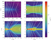 |
Fig. 1. Snapshots of the azimuthally averaged particle density (color) with attached poloidal magnetic field lines (white contours) and poloidal velocity stream (gray arrows). From left to right, the first snapshot is a large-scale view focusing on the cloud morphology significantly before the first core formation, while the three last snapshots zoom into the first core during and after its formation. |
The first snapshot is a large-scale view of the collapsing core. It illustrates how the magnetic field acts upon the infalling material: vertically, the motion is aligned with the field and the gas is free-falling. Radially, the misalignment generates a magnetic tension that slows the collapse. The result is a flattening of the core, as well as a pinching of the magnetic field lines that are dragged along the midplane by the gas. The clear interplay between gas motions and field line deformation is a result of the low diffusivities involved at this stage of the collapse. They are inefficient at decoupling the gas and the magnetic field, which remains in a near ideal MHD regime.
The three last snapshots focus on what happens at a small scale, just after the first hydrostatic core formation. As the core particle density increases, it reaches the critical value n1 (cf. Eq. (8)). The gas becomes adiabatic, which provides thermal support to the core that stops collapsing vertically (second snapshot). In the meantime, the radial collapse catches up and drags the magnetic field which acquires an hourglass shape. A torus-like, pressure-supported structure arises: it is the first hydrostatic core formation (third snapshot).
The large densities also increase the ambipolar and Ohmic diffusions. Inside the first core, the gas and the magnetic field are decoupled, and angular momentum accumulates. As a consequence, a small, rotationally supported disk settles (last snapshot). The newborn disk is fed by the remnant, vertically pressure-supported gas that could never reach the radial hydrostatic equilibrium. We refer to this midplane, pressure-supported gas as the “pseudo-disk” in the following. The “envelope” denomination is more generic and corresponds to any material that is not belonging to the disk or the seed.
3.2. disk secular evolution properties
In Fig. 2 we present the azimuthally averaged midplane surface density Σ, rotation rate Ω, poloidal magnetic field intensity BZ, and plasma parameter βP as a function of the radius, starting from the first core formation until the later times of the simulation.
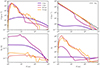 |
Fig. 2. Azimuthally averaged surface density (top left), rotation rate (top right), poloidal magnetic field intensity (bottom left), and plasma parameter βP (bottom right) versus the radius, computed in the midplane. Each color corresponds to one snapshot, the darker being the disk formation epoch, while the lighter is associated with the later times of the simulation. In the top right panel, the dashed black line is the theoretical Keplerian rotation rate with M⋆ ≈ 0.7 M⊙. |
We compute the surface density as  , where the density is integrated along the polar angle. The density barely contributes out of the disk, which itself covers a small θ range around the midplane. Therefore, this polar integration in spherical coordinates is a convenient approximation of the vertical integration in cylindrical coordinates.
At 5 kyr for R ≲ 10 au, the gas follows a steep power-law starting from a flat, high Σ. Further out, it follows a shallow power-law with low Σ. As time goes on, the steep power law becomes shallower while the transition radius increases up to 200 au.
The rotation rate is compared with the Keplerian prediction  with M⋆ the seed mass and R the cylindrical radius4. At 5 kyr for R ≲ 10 au, the gas is in Keplerian rotation. Further out, it is sub-Keplerian. As time goes on, the Keplerian transition radius increases up to 200 au. Thus, the steep, inner Σ region is associated with rotation-supported material while the outer shallow Σ region is sub-Keplerian.
At 5 kyr for R ≲ 10 au, the poloidal magnetic field shows a plateau. Further out, it follows a power-law. The intensity of the plateau decreases with time down to a few mG and the plateau transition radius increases up to a few 10 au. Initially, the plateau is associated with the rotation-supported, steep Σ region while the power-law is associated with the pressure-supported, shallow Σ region.
The plateau is characteristic of the non ideal MHD regime, responsible for decoupling the gas and BZ, while the power-law indicates a near ideal MHD regime due to the gas being less dense. A slight bump is observed at the transition radius and can be explained as follows: in the pseudo-disk region, BZ is dragged to inner radii by infalling material. Reaching the non ideal region, most of this field cannot be conveyed any further and piles up.
Finally, the plasma parameter is defined as βP = Pth/Pmag, where P is the thermal pressure and Pmag = B2/8π is the magnetic one. Thus, βP ≫ 1 indicates a thermally dominated gas, while βP ≪ 1 indicates a magnetically dominated one.
At 5 kyr for R ≲ 10 au, it follows a steep power-law starting from a high βP ≈ 105. Further out, the profile is slowly increasing from βP ≈ 1 and stays close to this limit value between the two regimes. Hence, there is a correlation between the magnetized, high surface density, rotationally supported gas, and the thermally dominated region.
As time goes on, the steep power law becomes shallower while the transition radius increases up to 200 au. The innermost region is even more thermally dominated, reaching βP ≈ 109. The outer region becomes magnetically dominated, with βP ≈ 10−1. We note that for any snapshot, the limit value βP ≈ 1 is located near the transition radius in the three other profiles.
3.3. Dynamics, size and mass repartition
The disk morphology is investigated in Fig. 3, which shows the gas surface density in the equatorial midplane at 5, 30, and 70 kyr. It covers the different dynamical states experienced by the disk during the secular integration: first, the disk is small and subject to spiral density waves. Second, it smoothes out and builds up, apart from one large, streamer-like spiral arm. Finally, the outer disk triggers new spirals that propagate to the inner radii.
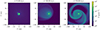 |
Fig. 3. Gas surface density in the equatorial plane. From left to right: three characteristic snapshots illustrating the successive behaviors of the disk at 5, 30, and 70 kyr respectively. |
In the middle panel, the disk exhibits a slightly eccentric morphology. We caution that this is probably a consequence of the fixed point mass assumption. In principle, while accreting mass with linear momentum, the point mass should move. Because this motion is not taken into account, there is a non-zero indirect term from gravity which makes the disk eccentric. That being said, we think it does not significantly affect the results, and the eccentricity disappears afterward (see right panel).
Figure 4 gives an overview of the evolution of the disk radius (Rd), the accretion rate (Ṁ) and the mass repartition between the seed (M⋆), the disk (Md) and the envelope (Menv) over the 100 kyr of the simulation.
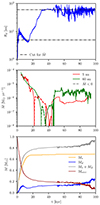 |
Fig. 4. Top panel: radius of the disk over time. The dash-dotted black lines emphasize the radii where the mass accretion rate is inspected in the next panel. Middle panel: mass accretion rate over time near the protostar (R = 5 au, red) and at the maximum stable outer radius (R = 60 au, green). Dashed lines correspond to expanding material. Bottom panel: protostar mass (orange), disk mass (blue), the total mass of the disk-protostar system (gray), and envelope mass (brown) over time. Data for the accretion rate are convolved in time using a 10 kyr window (equivalent to 8 orbits at 100 au). |
The top panel follows the evolution of the disk radius Rd. To compute it, we assume that cells satisfying uφ ≥ 0.9VK, uφ > uR and uφ > cs are part of the disk (VK and cs are the local Keplerian and sound velocities). The disk radius is then defined as the azimuthal median of the outermost radii that satisfy this criterion in the midplane.
As the disk forms after a few kyr, its radius reaches 10 au and immediately starts decreasing until 15 kyr. Then, it increases smoothly up to 60 au after 30 kyr where it remains constant until 45 kyr. After this point, the radius is subject to chaotic fluctuations around 60 au and remains so until the end of the simulation.
The middle panel follows the evolution of Ṁ near the protostar (R = 5 au) and at the maximum stable outer radius (R = 60 au). We perform an azimuthal integration over 2π and a vertical integration between ±H. In the following, H always refers to the disk geometrical scale height. Data are convolved in time using a 10 kyr window (equivalent to 8 orbits at 100 au). We caution that, in doing so, we smooth out short-timescale events occurring in the disk to focus on secular events. For instance, the fact that the accretion rate oscillates on the spiral dynamical timescale (Tomida et al. 2017) is verified, but hidden due to the large smoothing window.
We first focus on Ṁ(R = 5 au), which gives a good proxy for the accretion onto the protostar. As the disk forms, the protostar accretes at a strong rate of a few 10−5 M⊙ yr−1 that immediately starts decreasing until 20 kyr. There, it reverses with a negative rate around 10−6 M⊙ yr−11, which means that gas is expanding consistently with Rd and the protostar is no more accreting. After 35 kyr, the expansion episode stops and standard protostar accretion is back. It is first small, with strong variations between 10−8 and a few 10−7 M⊙ yr−1. After 45 kyr the range increases and stabilizes between a few 10−7 and 10−6 M⊙ yr−1.
For Ṁ(R = 60 au), the material is not part of the disk until 30 kyr and only marginally belongs to the disk afterward due to radius variability, such that we essentially probe the pseudo-disk accretion. As the disk forms, the pseudo-disk accretes at a strong rate of a few 10−5 M⊙ yr−1 that immediately start decreasing until 30 kyr. There, it reverses with a negative rate of a few 10−7 M⊙ yr−1. It is shortly and slightly expanding because Rd stops growing there. After 35 kyr, the expansion episode stops and standard pseudo-disk accretion is back. We note that the Ṁ(R = 60 au) is about one order of magnitude larger than Ṁ(R = 5 au), indicating that the disk density structure is still evolving and that proper steady state has not yet been reached.
Finally, the bottom panel shows the evolution of the mass repartition between the seed, the disk, and the envelope. M⋆ accounts for any mass falling below Rin. Md is computed by summing ρdV over any cell matching the disk criterion. The envelope mass is what is left of the initial 1 M⊙ cloud.
As the disk forms, M⋆ grows to 0.7 M⊙ until 15 kyr and stagnates afterward. In the meantime, Md reaches a maximum 0.15 M⊙ and immediately starts decreasing until 15 kyr. Then, it increases smoothly to 0.15 M⊙ after 30 kyr where it remains constant until 45 kyr. After this point, the disk mass keeps increasing while oscillating and remains so until the end of the simulation. The final disk mass is 0.25 M⊙.
Menv is rapidly decreasing until 10 kyr. Most of the lost mass ends up in the seed, the rest becomes part of the disk. After 5 kyr, the envelope mass becomes negligible compared to M⋆, and the decaying slope is shallower. The envelope is mainly accreted onto the disk. After 80 kyr, Menv becomes negligible compared to Md.
4. Accretion history
In this section, we study the accretion history of the disk based on the evolution of key physical quantities (surface density, magnetic field...). We isolate the main driving mechanisms for accretion, address their relevance throughout the disk evolution, and derive a comprehensive scenario over three accretion phases.
4.1. Driving accretion mechanisms
Protoplanetary disks are rotationally supported structures. In this context, accretion is only possible if there are one or several mechanisms capable of extracting angular momentum from the gas.
To properly account for each of these mechanisms, we derive the conservation of angular momentum in the cylindrical coordinates system (R, Z, φ) for the case of a self-gravitating, magnetized rotating disk (adapted from Lesur 2021a):
![Mathematical equation: $$ \begin{aligned} \overline{\rho u_R}\partial _R\left(\Omega R^2\right)+\frac{1}{R}\partial _R\left( R^2 \underbrace{\overline{\Pi _{R\varphi }}}_{\text{radial} \text{ stress}} \right)+R\underbrace{\left[ \langle \Pi _{Z\varphi } \rangle \right]_{-H}^{H}}_{\text{surface} \text{ stress}}=0, \end{aligned} $$](/articles/aa/full_html/2024/06/aa48405-23/aa48405-23-eq15.gif) (9)
(9)
with
 (10)
(10)
 (11)
(11)
where  , g is the gravitational field and
 (12)
(12)
for any quantity X and ![Mathematical equation: $ [X]_{-H}^H=X(Z=H)-X(Z=-H) $](/articles/aa/full_html/2024/06/aa48405-23/aa48405-23-eq20.gif) .
.
There are therefore six mechanisms acting upon the angular momentum transport in our case: hydrodynamical transport (first term in Eqs. (10) and (11)), gravitational transport (second term) and magnetic transport (third term), each of them generating both a radial stress (Eq. (10)) and a surface stress (Eq. (11)).
Among these quantities, we want to focus on the three main levers identified in previous works (Xu & Kunz 2021a,b) as the preponderant mechanisms at stake for such massive, embedded and magnetized disks: the radial gravitational stress GRφ, the magnetic braking MZφ (corresponding to the surface magnetic stress), and the surface hydrodynamical stress HZφ. Each of them is labeled as follows:
![Mathematical equation: $$ \begin{aligned}&G_{R\varphi }\equiv \frac{1}{R}\partial _R \left[R^2 \frac{\overline{g_R g_\varphi }}{4\pi G} \right],\end{aligned} $$](/articles/aa/full_html/2024/06/aa48405-23/aa48405-23-eq21.gif) (13)
(13)
![Mathematical equation: $$ \begin{aligned}&M_{Z\varphi }\equiv -R\left[\frac{\langle B_Z B_\varphi \rangle }{4\pi } \right]_{-H}^H,\end{aligned} $$](/articles/aa/full_html/2024/06/aa48405-23/aa48405-23-eq22.gif) (14)
(14)
![Mathematical equation: $$ \begin{aligned}&H_{Z\varphi }\equiv R\left[\langle \rho u_Z V_\varphi \rangle \right]_{-H}^H. \end{aligned} $$](/articles/aa/full_html/2024/06/aa48405-23/aa48405-23-eq23.gif) (15)
(15)
Figure 5 presents a comparison of each stress for three snapshots (with time increasing from top to bottom). A positive torque is associated with the extraction of angular momentum from the disk while a negative torque brings angular momentum to the disk.
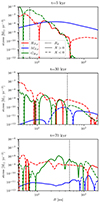 |
Fig. 5. From top to bottom we focus on t = 5, 30 and 70 kyr respectively. Each panel presents GRφ (green), MZφ (blue) and HZφ (red) versus the radius. Solid and dashed lines are associated with positive and negative stresses respectively. The dotted black line is the corresponding disk radius. Data are convolved in time using a 10 kyr window (equivalent to 8 orbits at 100 au). |
At 5 kyr, the gravitational stress is positive and dominant in the disk. It transports angular momentum from the inside out. In the meantime, magnetic braking is positive and dominant in the pseudo-disk. It extracts angular momentum from the gas. The hydrodynamical stress can be significant but is never dominant in the innermost 200 au.
At 30 kyr, the hydrodynamical stress is negative and dominant in the disk and inner pseudo-disk. It brings angular momentum from the envelope. In the meantime, magnetic braking is positive and dominant in the outer pseudo-disk. Yet, its intensity has significantly decreased. The gravitational stress can be significant but is never dominant in the innermost 200 au.
At 70 kyr, the hydrodynamical stress is negative and dominant in the inner disk. In the meantime, the gravitational stress is positive and dominant in the outer disk and the pseudo-disk. The magnetic braking is essentially positive but never significant in the innermost 200 au.
The relative importance of each stress can be connected with Fig. 6, which shows the accretion rate versus the radius for the same snapshots. Ṁ is computed as in the middle panel of Fig. 4. A positive rate corresponds to accretion while a negative one is associated with expansion.
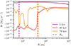 |
Fig. 6. Mass accretion rate versus the radius. Each color corresponds to one snaphsot at 5, 30 and 70 kyr respectively. The lighter, the later. Dashed lines represent the disk radius associated with each epoch. Data are convolved in time using a 10 kyr window (equivalent to 8 orbits at 100 au). |
At 5 kyr, both the disk and the pseudo-disk efficiently accrete at a few 10−5 M⊙ yr−1. At 30 kyr, the disk expands with Ṁ ranging between −10−7 and −10−6 M⊙ yr−1 and the pseudo-disk accretes at 10−6 M⊙ yr−1. The disk is therefore growing because of inside-out expansion and accumulation at the edge. At 70 kyr, the inner disk has no clear trend. It switches between accretion and expansion. In the meantime, the outer disk and the pseudo-disk accrete at Ṁ ∼ 10−6 M⊙ yr−1.
Accretion therefore results from the relative importance of each stress in the disk and the pseudo-disk. Understanding the secular evolution of these stresses is the key to understanding the different accretion behaviors.
4.2. Secular accretion scenario
In the following, we derive the disk accretion scenario in three phases by looking into the physical quantities underlying each stress.
First, spiral density waves are known to be an efficient angular momentum carrier. In our simulation, they are observed simultaneously with high accretion rates in the disk, making them a good candidate to explain accretion. Typically, Gravitational Instabilities (GI) are triggered when Md ≳ ϵM⋆ (Armitage 2011, Eq. (12)). The aspect ratio of the disk is ϵ ≲ 0.1 during the simulation, while Md > 0.1M⋆. Thus, our disk lies in the adequate regime, indicating that our spiral density waves are probably triggered by GI.
In order to characterize the stability of the disk with respect to its own gravity, we use a simplified version of the Toomre parameter Q (Toomre 1964; Goldreich & Lynden-Bell 1965a,b). Assuming that the gas is in Keplerian rotation, the simplified Toomre parameter QK writes as (Xu & Kunz 2021a,b):
 (16)
(16)
Many studies discuss the critical value for stability, which depends on the assumptions on the disk thickness or the perturbations linearity (Toomre 1964; Goldreich & Lynden-Bell 1965a,b; Gammie 2001; Wang et al. 2010). Based on these works, we expect the disk to be unstable when QK ∼ 1 while keeping in mind that the lower QK, the more likely the GI.
Second, the magnetic braking is a function of the poloidal magnetic field. Hence, the braking efficiency is controlled by the amount of poloidal magnetic flux stored in the gas. It is computed from the magnetic vector potential A:
 (17)
(17)
To complete our diagnostics, the hydrodynamical vertical stress is a function of the specific angular momentum j = Ruφ transported by the poloidal velocity flow Vp = uReR + uZeZ.
We present in Fig. 7 a series of spacetime diagrams connecting the surface density of the gas (top panel), the poloidal magnetic flux (middle panel), and the Toomre parameter (bottom panel). Figure 8 shows the specific angular momentum with the attached poloidal flow. We discuss below the different phases that we find from these figures.
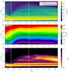 |
Fig. 7. Spacetime diagrams of the surface density (top panel), poloidal magnetic flux (middle panel), and Toomre parameter (bottom panel). Colors and radii are in log scale. The dashed white line corresponds to the disk radius, and dash-dotted white lines delimit the three accretion phases. Data were convolved in time using a 10 kyr window (equivalent to 8 orbits at 100 au). |
4.2.1. Phase I: A small, GI-driven disk
From the top panel of Fig. 7, we see that until 15 kyr, a high surface density region concentrates to the innermost 10 au corresponding to the disk. At the transition, there is a sharp drop in density, and the pseudo-disk is left with a low surface density. In parallel, the middle panel shows that a lot of magnetic flux is stored in the gas, especially within the pseudo-disk region, while the bottom panel presents a Toomre parameter that is of order of unity in the disk region, which is, therefore, GI unstable.
In addition, the left panel of Fig. 8 shows that the pseudo-disk provides material to the disk that has low specific angular momentum. At intermediate altitudes, the envelope provides material with higher j but does not reach the inner regions corresponding to the disk. At high altitudes, it provides material to the disk through its surfaces, but with low specific angular momentum.
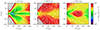 |
Fig. 8. From left to right we focus on t = 5, 30, and 70 kyr respectively, corresponding to each accretion phase. Each panel presents the specific angular momentum j in colors, with the attached poloidal velocity flow Vp as white quivers. |
Thus, in the first phase, the disk feeds the protostar thanks to GI-triggered spiral density waves that efficiently remove angular momentum at low radii. The instability is itself sustained by the mass influx from the pseudo-disk, driven by a powerful magnetic braking. There is a specific angular momentum contribution from the pseudo-disk and envelope to the disk, but it is not significant.
4.2.2. Phase II: Disk expansion fed by the envelope
From the top panel of Fig. 7, we see that between 15 and 45 kyr, the surface density increases at R ≳ 10 au, while the disk grows from inside out. This is synchronous with a continuous outward advection of the magnetic flux in the middle panel. We emphasize that at 10 au, ϕB decreases by roughly 2 orders of magnitude in the 20 first kyr. In the meantime, from the bottom panel, the Toomre parameter exhibits quite complex behavior. For R ≲ 10 au, QK is close to unity. This trend, along with the persistence of two low QK rings until the end of the simulation, predicts that the inner disk should trigger spiral density waves which we do not observe for these times and for these radii. Instead, two persistent ring-like features are observed in the surface density. Such rings are ubiquitous in self-gravitating disk simulations (Durisen et al. 2005; Boley et al. 2006; Michael et al. 2012; Steiman-Cameron et al. 2013, 2023) and are believed to be a common product of GI. Between 10 and 60 au, a significant decrease down to QK ∼ 5 is observed, as a response to the surface density increase, but this is not enough to enter a GI regime. The disk therefore smoothes out.
In addition, the middle panel of Fig. 8 shows that the pseudo-disk has become more efficient at providing angular momentum to the disk. At intermediate and high altitudes, the envelope now provides material with a large specific angular momentum, among which a significant part reaches the disk.
Thus, in the second phase, the disk stabilizes and smoothes out. It cannot accrete, since no angular momentum transport mechanism is efficient enough in this phase. On the contrary, it gains angular momentum from the envelope. The net result is a radial expansion of the disk, and the surface density power law becomes shallower. In the process, the accumulated magnetic flux is advected outward in a flux-freezing manner, hence a decrease in the magnetization. This is discussed in Sect. 4.3.
4.2.3. Phase III: GI-driven outer disk
From the top panel of Fig. 7, we see that the disk radius expansion is halted around 45 kyr and stabilizes at 60 au until the end of the simulation. In the meantime, the surface density front stops around 100 au, with a slight tendency to decrease by the end of the simulation. The flux outward advection in the middle panel stops as well, and there is even some late inward advection in the disk. In the bottom panel, at roughly 55 kyr, QK becomes of order of unity in the outermost part of the disk. The low value propagates to inner radii afterward, until the end of the simulation.
In addition, the right panel of Fig. 8 shows that the pseudo-disk starts to accrete low j material again. At intermediate altitudes, the specific angular momentum is the strongest, near the outer disk surfaces. From high altitudes, the envelope still provides material with significant j to the inner disk.
Thus, in the third phase, the disk does not receive enough angular momentum to keep expanding. The pseudo-disk is still braked and accretes onto the disk. The surface density profile steepens at the disk edge and triggers a new GI producing new spirals that propagate to inner radii. Hence the outer disk can accrete. This final state holds for the remaining 55 kyr suggesting that the disk ends up in a GI regulated state. We explore this idea in the following.
4.3. Flux-freezing during disk expansion
In Sect. 4.2.2, we find that while the disk is expanding, the magnetic flux is advected along with the gas consistently with a flux-freezing behavior. Here we discuss whether advection is indeed the dominant contribution to the magnetic field transport during the disk secular evolution. We define the midplane, azimuthally averaged, ideal, poloidal magnetic flux velocity transport  as (adapted from Lesur 2021b):
 (18)
(18)
where  comes from the first term of Eq. (7). Physically, it corresponds to the magnetic flux variation associated to advection.
Figure 9 presents  versus the radius for each phase, along with the location of the disk radius. It is normalized by the Keplerian velocity VK. A positive velocity is associated with outward transport while a negative velocity is associated with inward transport. In the following, we compare the prediction for the flux transport from advection only with the actual evolution from Fig. 7, middle panel. If they match, we conclude that the advection is mainly responsible for the flux transport, that is, the gas exhibits a flux-freezing behavior.
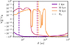 |
Fig. 9. Ideal magnetic flux velocity transport versus the radius. Each color corresponds to one snapshot at 5, 30, and 70 kyr respectively. The lighter, the later. Dashed lines represent the disk radius associated with each epoch. Data are convolved in time using a 10 kyr window (equivalent to 8 orbits at 100 au). |
At 5 kyr, the ideal transport predicts strong (≈ − 0.1) inward advection for the flux inside the disk, while we see it starts spreading in Fig. 7 (middle panel, phase I). Thus, diffusive transport dominates over advection. At 30 kyr, the ideal transport predicts significant (≈0.01) outward advection for the flux inside the disk, which is consistent with the flux recession in Fig. 7 (middle panel, phase II). Thus, the flux is advected by the spreading disk. At 70 kyr, the ideal transport predicts low (< 0.001) outward advection in the inner smooth disk and a slightly stronger (> 0.001) outward advection in the outer spiral-driven disk, while the flux seems slightly advected back inward on the long term in Fig. 7 (middle panel, phase III). This discrepancy suggests that accretion is not the main driver of flux transport in this phase.
Thus, we conclude that diffusion is responsible for flux leaking essentially during phase I and III. Conversely, during phase II, advection overcomes diffusion and the field is just diluted in the expanding disk.
4.4. A GI regulated final secular evolution
In Sect. 4.2, we conclude that the disk angular momentum process is dominated by GI-driven spiral density waves when accreting. Self-gravitating disks are prone to enter a marginally unstable, self regulated gravito-turbulent state where the Toomre parameter is maintained around the critical value Q ∼ 1 (Gammie 2001).
From Eq. (16), QK is controlled by two main levers: surface density Σ and temperature T (through  ). Yet, we use a barotropic EOS, such that T is set by the density. In this specific case, Xu & Kunz (2021a) argues that the disk stability is controlled by the surface density alone. It can enter GI through Σ increase, as a result of mass influx from the environment. Once unstable, such a disk can be brought back into stability only by lowering Σ, if authorized to spread or to significantly accrete.
To probe this phenomenon, we derive a critical surface density Σcr as a function of the radius, above which the disk should become unstable:
 (19)
(19)
where
![Mathematical equation: $$ \begin{aligned} \Sigma _0=\left[\frac{c_{\rm s,0}}{\pi }\sqrt{\frac{M_\star }{G}}(\epsilon \rho _1)^{(1-\gamma )/2} \right]^{2/(3-\gamma )}\approx 2\times 10^{5} \, \mathrm g \, cm^{-2} , \end{aligned} $$](/articles/aa/full_html/2024/06/aa48405-23/aa48405-23-eq32.gif) (20)
(20)
with ρ1 = n1 ⋅ mn the critical mass density for which the gas becomes adiabatic.
Σcr is calculated from Eq. (16) with the following assumptions:
-
QK = 1.
-
 (adiabatic regime).
 -
 .
.
Most of the data used for the calculation are detailed in Sects. 2.3 and 2.6, and we take γ = 1.4, ϵ = 0.1 and M⋆ = 0.7 M⊙.
The critical surface density is reported as a dashed black line in Fig. 10, along with the measured disk surface density for three snapshots spanning over each phase.
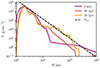 |
Fig. 10. disk surface density versus the radius. Each color focuses on one accretion phase at 5, 30, and 70 kyr respectively. The lighter, the later. The dashed black line is the predicted critical surface density from Eq. (19). |
At 5 kyr, the steep power-law at R ≲ 10 au matches the critical value between 2 and 4 au, and stands below further out. This is consistent with the spiral-driven disk in phase I. At 30 kyr, the power-law spreads, while staying below Σcr. This is consistent with the smooth disks in phase II. At 70 kyr, the inner disk stands below the critical surface density while the outer disk saturates at Σcr, around which it oscillates. This is consistent with the spiral-driven outer disk in phase III.
Hence, any deviation from the stability regime enforced by self-gravity leads to negative feedback that promotes accretion. In this sense, the disk is shaped by self-gravity. In the case where a sustained influx of material increases locally the surface density, the disk enters a self regulated state where Rd stabilizes around 60 au. This emphasizes the role of the environment interacting with the disk.
5. Interaction with the parent molecular cloud: A large-scale accretion streamer
The most striking evidence of an interaction between the molecular cloud and the protostar-disk system is the appearance of a large-scale, streamer-like spiral arm driving asymmetric infall between the remnant cloud and the central protostar-disk system. Here, we discuss the accretion streamer morphology and kinematics and investigate on how it connects to the central system. We also compute some observational properties.
5.1. Streamer spatial and velocity distribution: A sheet-like morphology
Figure 11 presents a large-scale equatorial slice of the gas surface density (top row) along with poloidal slices of the gas particle density (middle row) and poloidal velocity (bottom row) performed at the azimuth of the streamer for two late time snapshots. The poloidal velocity is normalized by the free-fall velocity  .
.
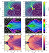 |
Fig. 11. Top row: large-scale equatorial slice of the gas surface density with associated equatorial velocity flow (white quivers). A dashed white line indicates the azimuth of the main streamer, for which poloidal slices are performed. Middle row: large-scale poloidal slice of the gas particle density with associated poloidal velocity flow (white quivers). Bottom row: large-scale poloidal slice of the gas poloidal velocity, normalized by the free-fall velocity, with associated poloidal velocity flow (white quivers). Each column corresponds to a late time snapshot, respectively at 60 (left column) and 70 kyr (right column). In each plot, a line integrated convolution treatment is applied to emphasize the gas streamlines. The innermost 100 au are masked by a gray circle to allow for adequate contrast. |
Focusing on the top row, we see that the environment of the protostar-disk system is divided between a low surface density bubble and an extended region of growing surface density that culminates in an azimuthally localized channel of gas at lower radii. This is the main accretion streamer, toward which the equatorial velocity flow is converging. The streamer structure extends up to approximately 1000 au and connects to the disk. A second converging flow is observed in the low-density bubble, corresponding to an additional fainter streamer. The streamers rotate between the two snapshots.
The middle row shows that the gas particle density is vertically stratified, with densities ranging between 106 cm−3 close to the polar axis and 108 cm−3 in the midplane. Overall, the streamer converges in a sheet-like morphology that is even better identified when represented in three dimensions5.
Finally, the bottom row illustrates two different dynamical behaviors. Far from the midplane, the flow is near free-fall. The gas is channeled toward lower radii at constant velocity and falls directly above (and below) the disk. Near the midplane, the large-scale velocity is smaller. A gradient is observed toward lower radii as the gas catches up with more elevated material, reaching near free-fall velocity. In this case, the gas falls directly onto the disk edge. The associated velocity variation suggests that material is shocking in this region.
In Fig. 12, we present a large-scale equatorial slice at t = 60 kyr showing the plasma parameter βP. Interestingly, the streamer and the central protostar-disk system are characterized by βP > 1, indicating that the gas in these regions is thermally dominated. On the contrary, the surrounding low-density bubble is characterized by βP < 1, indicating that the gas is magnetically dominated. This configuration points toward a magnetic origin for the streamer formation, such as the interchange instability proposed by Mignon-Risse et al. (2021) in the context of massive star formation or the magnetic process discussed in Tu et al. (2023) for the collapse of a turbulent, low-mass protostellar core.
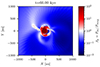 |
Fig. 12. Large-scale equatorial slice at t = 60 kyr. Colors are the plasma parameter βP. |
5.2. Connecting to the central system: Looking for shock signatures
Figure 13 provides a three-dimensional representation of the disk and streamer with two attached streamlines at time 70 kyr. The disk and streamer are displayed for representation purposes. In this plot, cells associated with the disk must have gas particle density over 109 cm−3. The streamer corresponds to cells where n ≥ 106 cm−3 and ur < 0 to ensure we focus on infalling material belonging to the parent molecular cloud. We additionally require r > 200 au to exclude the central system. Streamlines are integrated with starting points of cylindrical radius R0 = 350 au and azimuth φ0 = φstreamer, with respectively Z0 = 0 and Z0 = 100 au to probe the gas in the midplane and at elevated location.
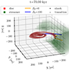 |
Fig. 13. Three-dimensional representation of the disk and streamer with two attached streamlines at time 70 kyr. Red surfaces correspond to the disk, while green surfaces represent the streamer. Both streamlines start at R = 350 au and φ = φstreamer with respectively Z = 0 (orange solid line) and Z = 100 au (blue solid line). Black dots indicate shocks (or rarefactions) along the streamlines while the gray dot corresponds to a density transition (see Fig. 14 for their identification). For an animated version of the figure with a large-scale visualization of the streamer, see https://cloud.univ-grenoble-alpes.fr/s/ZNwHrbWg8A24Trb. |
The midplane streamline remains in the streamer and the midplane until it reaches the large-scale spiral arm where it is abruptly deflected (see Fig. 14) and entrained in the spiral motion. In contrast, the elevated streamline is channeled directly onto the innermost part of the disk, if not directly falling onto the seed (see the animated version of the plot for a better understanding).
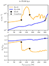 |
Fig. 14. Top: particle density along the streamlines starting at Z0 = 0 au and Z0 = 100 au respectively. Bottom: Gas velocity projected along each streamline. Colors and dots are the same as in Fig. 13. |
The question of the shock is addressed by Fig. 14. The top panel shows the gas particle density in the streamline as a function of the position on the streamline while the bottom panel is the normalized gas velocity parallel to the streamline V∥/Vff.
For the midplane streamline, a first shock signature is observed at 100 au with both discontinuities in density and velocity consistent with the encounter between the streamer and the spiral arm. The density jumps from roughly 108 to almost 1010 cm−3 and the gas loses more than half of its velocity. A fainter secondary rarefaction signature is observed around 170 au where density and velocity drop again. We caution that the gas is not in a steady state, hence the streamline may not be representative of the gas kinematics after the first deflection. For the elevated streamline, we observe a sharp increase in density corresponding to the moment where the gas connects with the disk. However, the velocity along the streamline remains near free-fall at any position, and only a faint, smooth velocity gradient is observed. This corresponds to a smooth density transition, rather than a shock signature.
5.3. Streamer mass and infall rate: Impact on protostar-disk accretion
To close our analysis of the streamer, we compute its mass and infall rate. We stay as close as possible to the computation method provided by Valdivia-Mena et al. (2022).
We stick to the definition in Sect. 5.2 to flag cells belonging to the streamer. The mass is then computed by summing ρdV over each cell. We obtain Mstreamer ≈ 0.02 M⊙ corresponding to 3% of the protostar’s mass and 10% of the disk mass at 70 kyr.
The infall rate Ṁin is the mass rate at which the streamer is infalling onto the protostar-disk system. It is not to be confused with the accretion rate Ṁ⋆ directly onto the protostar. Valdivia-Mena et al. (2022) compute it through Ṁin = Mstreamer/tff,streamer where tff, streamer is computed using a streamline model. On each point of the streamline, they interpolate the velocity V∥ and length variation dl. They can therefore compute the time needed to reach the disk.
We do the same using a streamline starting at (R, Z, φ) = (Rstreamer, 0, φstreamer), with Rstreamer ≈ 1400 au the outermost radius of the streamer. We then sum dl/V∥ along the streamline to get tff,streamer ≈ 13 kyr giving Ṁin ≈ 1.5 × 10⁻⁶ M⊙ yr−1. Compared to the accretion rate Ṁ⋆ ≡ Ṁ(R = 5 au) ≈ 5 × 10⁻⁷ M⊙ yr−1 at the same time, we get a ratio of infall to accretion of Ṁin/Ṁ⋆ ≈ 3.
6. Discussion
In this section, we confront our disk secular evolution and final GI regulated state with observations. We also discuss the compatibility of our accretion streamer with what is observed by comparing its properties with the literature.
6.1. disk secular evolution and GI self regulation
In the first 15 kyr of its life, the newborn disk is small, compact, and magnetized. It lies in the non ideal regime and accretes through GI-driven spiral density waves. This is because efficient magnetic braking promotes accretion in the well-coupled MHD pseudo-disk, which in return increases the disk mass and makes it unstable. During the second phase, between 15 and 45 kyr, the accretion in the pseudo-disk becomes less efficient and the disk can stabilize. In the meantime, the envelope provides high angular momentum material to the disk that can therefore expand. As a result, the accumulated magnetic flux is advected outward and magnetization decreases. In the third phase, lasting for the remaining 55 kyr, expansion is halted in the disk and mass accumulates at the edge from the pseudo-disk. At some point, the outer disk is massive enough to be unstable and the disk’s final state is GI regulated.
As a complement, we would like to emphasize an interesting result regarding the plasma parameter βP. In Sect. 4.2, we find that during phase II the disk is expanding, and its magnetic flux is advected along with the gas. In such a case, assuming the disk mass Md and poloidal magnetic flux ϕd to be constant, one can show that  . This is verified in Fig. 2, bottom right panel. At 5 kyr, βP(Rd)≈10. Later on, once the disk radius has increased by roughly one order of magnitude, the associated plasma parameter is βP(Rd)≈103. The verified dependency is a confirmation that once a given amount of flux is stored in the disk, it follows the gas evolution, and magnetization evolves accordingly.
Numerically speaking, our collapse and disk’s early evolution are in line with other works. Magnetic decoupling occurs by the time of the first core formation leading to a plateau with Bz ≃ 100 mG threading the disk, as expected in core-collapse simulations including ambipolar diffusion (Masson et al. 2016; Vaytet et al. 2018; Xu & Kunz 2021b). The initial disk size of roughly 10 au is consistent with a magnetic regulation (Hennebelle et al. 2016). A decreased magnetization is then observed for simulations that properly resolve the disk vertical extent (Xu & Kunz 2021b). The disk becomes massive and resistive enough to be gravitationally regulated (Tomida et al. 2017; Xu & Kunz 2021a,b). The piling up of magnetic field at the transition between the diffusive and ideal MHD regimes is reminiscent of the magnetic wall proposed by Li & McKee (1996) and observed also in Xu & Kunz (2021b), though with a fainter accumulation that could be explained by the differences in the diffusivity tables.
On the observational side, resolution is often missing to infer the surface density profile in class 0/I systems and we lack robust tracers to unveil the magnetization. The few studies available for the surface density find a power-law index between −1.7 and −1.5 (Yen et al. 2014; Aso et al. 2015, 2017). This is shallower than what we constrain to justify our GI regulation mechanism (≈ − 2). On the other hand, Fiorellino et al. (2023) find that many class I have a disk-to-star mass ratio above 0.1, which they claim is typical for a GI regulated disk. That being said, spirals are observed in only a few class 0/I protostars (Tobin et al. 2018; Lee et al. 2020), while most of these objects do not show structures (Ohashi et al. 2023). Yet, it is worth mentioning that these disks can be optically thick, in which case the spirals can be hidden.
The Class II stage is slightly better constrained. The review from Andrews (2020) summarizes class II disk properties inferred from observations. The constrained surface density profile has an index of ≈ − 1, again shallower than our finding, making GI regulation unlikely. Conversely, Zeeman measurements of the poloidal magnetic field give an upper limit of ∼1 mG at a few 10 au (Vlemmings et al. 2019) consistent with our final disk magnetization.
Thus, most of the properties of our evolved disk are consistent with current observations, with the exception of the GI regulated state, characterized by a steep surface density profile and prominent spiral density waves, which seem to be uncommon, even in young disks. The inclusion of internal heating, which is missing in the current model, could help stabilize the disk. Yet, it would not change the final picture. Indeed, in our simulation, the triggering of GI is inevitable when magnetic braking is neutralized by an inefficient magnetic coupling because no other mechanism is able to evacuate the disk angular momentum as mass piles up.
This however ignores the role of MHD disk winds that could be launched from the ionized surface layers of the disk. In our simulation, a large-scale outflowing structure arises, but it is launched far from the disk surface. The importance of such outflows with elevated launching points is discussed in many core-collapse simulations (Machida & Hosokawa 2013; Tsukamoto et al. 2015; Masson et al. 2016; Marchand et al. 2020) and they are proposed as a means to redistribute angular momentum. However, in our simulation, we find that the outflow is launched from a low density region (a “vacuum”) which density is set by the numerical limiters (Alfvén and density floor). Therefore, in our view, its origin remains numerical.
Hence, we conclude that no proper MHD disk wind is found in our simulation, while many “disk only” simulations including surface ionization exhibit MHD disk winds (Béthune et al. 2017; Bai & Stone 2017; Suriano et al. 2019; Lesur 2021b). These surface ionization processes are due to stellar far UV and X-ray photons that increase the ionization fraction by orders of magnitude. These effects are absent in our simulation, in which we only consider cosmic ray ionization in our chemical network. Hence it is tempting to associate the GI regulated disk we obtain to the lack of stellar irradiation at the disk surface. This possibility should be investigated in the future.
6.2. Large-scale streamer driving accretion in the envelope
The long-term interaction of the envelope with the protostar-disk system leads to the formation of an accretion streamer. It is composed of near free-fall gas organized in a sheet-like configuration. It connects to the protostar-disk system either by shocking onto the disk edge in the midplane or by smoothly accreting onto the disk surfaces from higher altitudes. Quantitatively, the streamer maximum radius is ≈1400 au with mass and infall rates of 0.02 M⊙ and 1.5 × 10⁻⁶ M⊙ yr−1, corresponding to 3% of the seed mass and 3 times the protostar accretion respectively.
Asymmetric large-scale structures are ubiquitous in numerical core-collapse models with sufficiently massive molecular clouds, accounting for turbulence (Kuffmeier et al. 2017; Lam et al. 2019; Kuznetsova et al. 2019; Wurster et al. 2019; Lebreuilly et al. 2021) or not (Mignon-Risse et al. 2021). The resulting envelope is often messy, exhibiting streamers with filamentary or sheet-like morphologies. Tu et al. (2023) propose a magnetic origin of the streamer formation, which is also supported by Mignon-Risse et al. (2021) and consistent with our work.
Accretion streamers have been observed both in deeply embedded class 0 (Pineda et al. 2020; Murillo et al. 2022) and in class I sources (Yen et al. 2019; Valdivia-Mena et al. 2022; Hsieh et al. 2023). They are rotating, free-falling, and connect to the disk (Pineda et al. 2020; Valdivia-Mena et al. 2022). The meeting point is either associated with a smooth transition between the infalling streamer velocity and the Keplerian disk velocity (Yen et al. 2019; Pineda et al. 2020) or it can present a sharp velocity drop consistent with shock tracing signatures (Valdivia-Mena et al. 2022). It is remarkable that both these conclusions are in agreement with the kinematics in our streamer.
A large variety of streamer sizes have been observed (103 − 104 au). The streamer mass ranges between 10−3 and 10−1 M⊙, and can be a significant fraction of the protostellar mass (0.1 − 10% of M⋆, Pineda et al. 2020; Valdivia-Mena et al. 2022; Hsieh et al. 2023). The infall rate of the streamer is Ṁin = 10−6 M⊙ yr−1, and can be of the same order as the protostellar accretion rate Ṁ⋆, if not higher. Pineda et al. (2020), Valdivia-Mena et al. (2022), Hsieh et al. (2023) find Ṁin/Ṁ⋆ ≈ 1, 5 − 10 and ≥0.05 respectively. Our computations are all lying in the observed range.
7. Conclusion
We performed a 3D large timescale, non ideal core collapse simulation in order to probe the secular evolution of embedded protoplanetary disks while paying specific attention to the magnetic field evolution and the disk’s long-term interaction with the surrounding infalling envelope.
We follow the cloud collapse until the first hydrostatic core formation leading to disk settling and integrate for an additional 100 kyr. The simulation lasts for about 20% of the class I stage (Evans et al. 2009). Yet in the meantime, 90% of the envelope is accreted by the seed or onto the disk, pointing toward an ending class I. This faster evolution of the numerical model with respect to the observations is probably a consequence of the dynamically unstable initial condition.
We achieve a resolution of 10 cells per scale height (assuming ϵ = 0.1) in order to properly capture magnetic field diffusion, field line twisting, and GI induced spirals. Our main results are:
-
The disk experiences three accretion phases. In particular, once the disk has settled, magnetic braking mainly controls accretion in the pseudo-disk. Conversely, self-gravity controls angular momentum transport in the disk through spiral density waves triggered via Toomre instability. When gas is expanding, it is thanks to the envelope providing high angular momentum material through the disk surfaces.
-
During phase II, the disk expands while keeping its mass and flux roughly constant. As a result, the plasma parameter at the disk edge follows
 . This dependency is evidence that the initial amount of magnetic flux is conserved throughout the disk evolution, and magnetization evolves accordingly to the gas motion.
 -
The disk ends up in a GI regulated state maintaining Rd around 60 au. Its surface density profile is shaped by a critical surface density radial profile of index ≈ − 2.
-
The early evolution of the disk reproduces well the results from core-collapse models such as disk compacity, magnetic field decoupling, magnetic and later GI regulation. However, no MHD disk wind is found in our simulation. This is a natural outcome of efficient decoupling, yet it contrasts with disk-only models that systematically find MHD disk winds. We conjecture that this could be due to a lack of stellar ionization processes.
-
The expanding Keplerian gas and the decrease of the magnetic field qualitatively match class II observations. Yet, the observed power-law surface density is too steep to trigger gravitational instabilities, and the presence of Toomre-driven spirals is not supported by observations.
-
After 30 kyr, the envelope is organized in a large-scale, sheet-like accretion streamer that feeds the disk. It smoothly connects to its surfaces from elevated locations and shocks onto the outer rim in the midplane. It is a significant reservoir of mass whose infall rate is comparable to the accretion rate of the protostar.
In conclusion, this secular run shows that the neutralization of magnetic braking due to an efficient decoupling leads the disk to a nearly pure hydrodynamical state where GI is the only means to accrete. Consequently, the disk is stuck in a GI regulated state shaping its surface density profile and final radius.
Yet, this scenario is difficult to support, due to the lack of observed spirals in embedded systems. This suggests that current models overestimate the importance of diffusion after disk formation. It would be interesting to explore additional ionization processes susceptible to recovering a magnetically dominated accretion. The choice of initial conditions and the impact of grain size may also act upon the diffusions. This will be the topic of a forthcoming paper.
ρ0 ≈ 9 × 10⁻¹⁸ g cm−3.
We assume a mean mass per neutral particle mn = 2.33mp, corresponding to the composition of the solar nebula.
 . The core is therefore supercritical (μ > 1).
ΩK is derived taking M⋆ at 50 kyr, because M⋆ is roughly constant afterward.
A 3D model of the streamer at 70 kyr based on particle density contours is available on https://sketchfab.com/3d-models/streamer-1407-fid-66107da9c4854078aadac140de9f4e73
Acknowledgments
We wish to thank our anonymous referee for valuable comments and suggestions that improved the present paper. We are thankful to Matthew Kunz, Benoit Commerçon and Patrick Hennebelle for fruitful discussions about the physics of collapsing cores. This project has received funding from the European Research Council (ERC) under the European Union’s Horizon 2020 research and innovation program (Grant Agreement No. 815559 (MHdisks)). This work was supported by the “Programme National de Physique Stellaire” (PNPS), “Programme National Soleil-Terre” (PNST), “Programme National de Hautes Energies” (PNHE), and “Programme National de Planétologie” (PNP) of CNRS/INSU co-funded by CEA and CNES. This work was granted access to the HPC resources of IDRIS under the allocation 2023-A0140402231. Some of the computations presented in this paper were performed using the GRICAD infrastructure (https://gricad.univ-grenoble-alpes.fr), which is supported by Grenoble research communities. Data analysis and visualization in the paper were conducted using the scientific Python ecosystem, including numpy (Harris et al. 2020), scipy (Virtanen et al. 2020) and matplotlib (Hunter 2007).
References
- Andrews, S. M. 2020, ARA&A, 58, 483 [Google Scholar]
- Armitage, P. J. 2011, ARA&A, 49, 195 [Google Scholar]
- Aso, Y., Ohashi, N., Saigo, K., et al. 2015, ApJ, 812, 27 [Google Scholar]
- Aso, Y., Ohashi, N., Aikawa, Y., et al. 2017, ApJ, 849, 56 [NASA ADS] [CrossRef] [Google Scholar]
- Bai, X.-N., & Stone, J. M. 2017, ApJ, 836, 46 [Google Scholar]
- Béthune, W., & Rafikov, R. R. 2019, MNRAS, 487, 2319 [Google Scholar]
- Béthune, W., Lesur, G., & Ferreira, J. 2017, A&A, 600, A75 [NASA ADS] [CrossRef] [EDP Sciences] [Google Scholar]
- Boley, A. C., Mejía, A. C., Durisen, R. H., et al. 2006, ApJ, 651, 517 [Google Scholar]
- Durisen, R. H., Cai, K., Mejía, A. C., & Pickett, M. K. 2005, Icarus, 173, 417 [NASA ADS] [CrossRef] [Google Scholar]
- Evans, C. R., & Hawley, J. F. 1988, ApJ, 332, 659 [Google Scholar]
- Evans, N. J., Dunham, M. M., Jørgensen, J. K., et al. 2009, ApJS, 181, 321 [NASA ADS] [CrossRef] [Google Scholar]
- Fiorellino, E., Tychoniec, Ł., de Miera, F. C.-S., et al. 2023, ApJ, 944, 135 [NASA ADS] [CrossRef] [Google Scholar]
- Gammie, C. F. 2001, ApJ, 553, 174 [Google Scholar]
- Goldreich, P., & Lynden-Bell, D. 1965a, MNRAS, 130, 97 [NASA ADS] [CrossRef] [Google Scholar]
- Goldreich, P., & Lynden-Bell, D. 1965b, MNRAS, 130, 125 [Google Scholar]
- Harris, C. R., Millman, K. J., van der Walt, S. J., et al. 2020, Nature, 585, 357 [NASA ADS] [CrossRef] [Google Scholar]
- Hennebelle, P., Commerçon, B., Chabrier, G., & Marchand, P. 2016, ApJ, 830, L8 [Google Scholar]
- Hsieh, T.-H., Segura-Cox, D., Pineda, J., et al. 2023, A&A, 669, A137 [NASA ADS] [CrossRef] [EDP Sciences] [Google Scholar]
- Hunter, J. D. 2007, Comput. Sci. Eng., 9, 90 [NASA ADS] [CrossRef] [Google Scholar]
- Kuffmeier, M., Haugbølle, T., & Nordlund, Å. 2017, ApJ, 846, 7 [NASA ADS] [CrossRef] [Google Scholar]
- Kunz, M. W., & Mouschovias, T. C. 2009, ApJ, 693, 1895 [Google Scholar]
- Kuznetsova, A., Hartmann, L., & Heitsch, F. 2019, ApJ, 876, 33 [NASA ADS] [CrossRef] [Google Scholar]
- Lam, K. H., Li, Z.-Y., Chen, C.-Y., et al. 2019, MNRAS, 489, 5326 [NASA ADS] [CrossRef] [Google Scholar]
- Lebreuilly, U., Hennebelle, P., Colman, T., et al. 2021, ApJ, 917, L10 [NASA ADS] [CrossRef] [Google Scholar]
- Lee, C.-F., Li, Z.-Y., & Turner, N. J. 2020, Nat. Astron., 4, 142 [CrossRef] [Google Scholar]
- Lesur, G. R. 2021a, J. Plasma Phys., 87, 205870101 [CrossRef] [Google Scholar]
- Lesur, G. R. 2021b, A&A, 650, A35 [NASA ADS] [CrossRef] [EDP Sciences] [Google Scholar]
- Lesur, G., Baghdadi, S., Wafflard-Fernandez, G., et al. 2023, A&A, 677, A9 [NASA ADS] [CrossRef] [EDP Sciences] [Google Scholar]
- Li, Z.-Y., & McKee, C. F. 1996, ApJ., 464, 373 [NASA ADS] [CrossRef] [Google Scholar]
- Lubow, S., Papaloizou, J., & Pringle, J. 1994, MNRAS, 267, 235 [NASA ADS] [CrossRef] [Google Scholar]
- Machida, M. N., & Hosokawa, T. 2013, MNRAS, 431, 1719 [NASA ADS] [CrossRef] [Google Scholar]
- Marchand, P., Masson, J., Chabrier, G., et al. 2016, A&A, 592, A18 [NASA ADS] [CrossRef] [EDP Sciences] [Google Scholar]
- Marchand, P., Tomida, K., Tanaka, K. E., Commerçon, B., & Chabrier, G. 2020, ApJ, 900, 180 [CrossRef] [Google Scholar]
- Maret, S., & Bergin, E. A. 2015, Astrophysics Source Code Library [record ascl:1507] [Google Scholar]
- Maret, S., Maury, A., Belloche, A., et al. 2020, A&A, 635, A15 [NASA ADS] [CrossRef] [EDP Sciences] [Google Scholar]
- Masson, J., Chabrier, G., Hennebelle, P., Vaytet, N., & Commerçon, B. 2016, A&A, 587, A32 [NASA ADS] [CrossRef] [EDP Sciences] [Google Scholar]
- Maury, A., André, P., Testi, L., et al. 2019, A&A, 621, A76 [NASA ADS] [CrossRef] [EDP Sciences] [Google Scholar]
- Meyer, C. D., Balsara, D. S., & Aslam, T. D. 2014, J. Comput. Phys., 257, 594 [NASA ADS] [CrossRef] [Google Scholar]
- Michael, S., Steiman-Cameron, T. Y., Durisen, R. H., & Boley, A. C. 2012, ApJ, 746, 98 [Google Scholar]
- Mignon-Risse, R., González, M., Commerçon, B., & Rosdahl, J. 2021, A&A, 652, A69 [NASA ADS] [CrossRef] [EDP Sciences] [Google Scholar]
- Mouschovias, T. C., & Spitzer, L., Jr 1976, ApJ, 210, 326 [NASA ADS] [CrossRef] [Google Scholar]
- Murillo, N. M., van Dishoeck, E. F., Hacar, A., Harsono, D., & Jørgensen, J. K. 2022, A&A, 658, A53 [NASA ADS] [CrossRef] [EDP Sciences] [Google Scholar]
- Ohashi, N., Tobin, J. J., Jørgensen, J. K., et al. 2023, ApJ, 951, 8 [NASA ADS] [CrossRef] [Google Scholar]
- Pineda, J. E., Segura-Cox, D., Caselli, P., et al. 2020, Nat. Astron., 4, 1158 [NASA ADS] [CrossRef] [Google Scholar]
- Price, D. J., & Bate, M. R. 2007, Ap&SS, 311, 75 [NASA ADS] [CrossRef] [Google Scholar]
- Sheehan, P. D., Tobin, J. J., Looney, L. W., & Megeath, S. T. 2022, ApJ, 929, 76 [NASA ADS] [CrossRef] [Google Scholar]
- Steiman-Cameron, T. Y., Durisen, R. H., Boley, A. C., Michael, S., & McConnell, C. R. 2013, ApJ, 768, 192 [Google Scholar]
- Steiman-Cameron, T. Y., Durisen, R. H., Boley, A. C., et al. 2023, ApJ, 958, 139 [NASA ADS] [CrossRef] [Google Scholar]
- Suriano, S. S., Li, Z.-Y., Krasnopolsky, R., Suzuki, T. K., & Shang, H. 2019, MNRAS, 484, 107 [NASA ADS] [CrossRef] [Google Scholar]
- Tobin, J. J., Looney, L. W., Li, Z.-Y., et al. 2018, ApJ, 867, 43 [CrossRef] [Google Scholar]
- Tobin, J. J., Sheehan, P. D., Megeath, S. T., et al. 2020, ApJ, 890, 130 [CrossRef] [Google Scholar]
- Tomida, K., Machida, M. N., Hosokawa, T., Sakurai, Y., & Lin, C. H. 2017, ApJ, 835, L11 [Google Scholar]
- Toomre, A. 1964, ApJ, 139, 1217 [Google Scholar]
- Toro, E. F. 2009, Riemann Solvers and Numerical Methods for Fluid Dynamics: A Practical Introduction (Springer), 315 [CrossRef] [Google Scholar]
- Trott, C. R., Lebrun-Grandié, D., Arndt, D., et al. 2022, IEEE Trans. Parallel Distrib. Syst., 33, 805 [CrossRef] [Google Scholar]
- Tsukamoto, Y., Iwasaki, K., Okuzumi, S., Machida, M. N., & Inutsuka, S.-I. 2015, MNRAS, 452, 278 [NASA ADS] [CrossRef] [Google Scholar]
- Tsukamoto, Y., Maury, A., Commerçon, B., et al. 2022, arXiv e-prints [arXiv:2209.13765] [Google Scholar]
- Tu, Y., Li, Z. Y., Lam, K. H., Tomida, K., & Hsu, C. Y. 2023, arXiv e-prints [arXiv:2307.16774] [Google Scholar]
- Umebayashi, T., & Nakano, T. 1990, MNRAS, 243, 103 [NASA ADS] [CrossRef] [Google Scholar]
- Vaidya, B., Prasad, D., Mignone, A., Sharma, P., & Rickler, L. 2017, MNRAS, 472, 3147 [NASA ADS] [CrossRef] [Google Scholar]
- Valdivia-Mena, M., Pineda, J., Segura-Cox, D., et al. 2022, A&A, 667, A12 [NASA ADS] [CrossRef] [EDP Sciences] [Google Scholar]
- Vaytet, N., Commerçon, B., Masson, J., González, M., & Chabrier, G. 2018, A&A, 615, A5 [NASA ADS] [CrossRef] [EDP Sciences] [Google Scholar]
- Virtanen, P., Gommers, R., Oliphant, T. E., et al. 2020, Nat. Methods, 17, 261 [Google Scholar]
- Vlemmings, W., Lankhaar, B., Cazzoletti, P., et al. 2019, A&A, 624, L7 [NASA ADS] [CrossRef] [EDP Sciences] [Google Scholar]
- Wang, H.-H., Klessen, R. S., Dullemond, C. P., Van Den Bosch, F. C., & Fuchs, B. 2010, MNRAS, 407, 705 [CrossRef] [Google Scholar]
- Wurster, J., Bate, M. R., & Price, D. J. 2019, MNRAS, 489, 1719 [NASA ADS] [CrossRef] [Google Scholar]
- Xu, W., & Kunz, M. W. 2021a, MNRAS, 502, 4911 [NASA ADS] [CrossRef] [Google Scholar]
- Xu, W., & Kunz, M. W. 2021b, MNRAS, 508, 2142 [NASA ADS] [CrossRef] [Google Scholar]
- Yen, H.-W., Takakuwa, S., Ohashi, N., et al. 2014, ApJ, 793, 1 [NASA ADS] [CrossRef] [Google Scholar]
- Yen, H.-W., Gu, P.-G., Hirano, N., et al. 2019, ApJ, 880, 69 [NASA ADS] [CrossRef] [Google Scholar]
- Zhang, B., Sorathia, K. A., Lyon, J. G., Merkin, V. G., & Wiltberger, M. 2019, J. Comput. Phys., 376, 276 [NASA ADS] [CrossRef] [Google Scholar]
- Zhu, Z., & Stone, J. M. 2018, ApJ, 857, 34 [Google Scholar]
Appendix A: Self-gravity solver
A.1. Implementation in IDEFIX
The IDEFIX code is upgraded with a self-gravity module. By resolving Eq. (6), it infers the self-gravitational potential from the gas density distribution.
The Laplacian operator is discretized using second-order finite difference with self-consistent boundary conditions. The resulting matricial system is solved iteratively by a biconjugate gradient stabilized (BICGSTAB) algorithm. It uses the KOKKOS routines encapsulated in IDEFIX to handle parallelization (Trott et al. 2022; Lesur et al. 2023).
A Jacobian preconditioner P can be used to fasten convergence. It is designed as the diagonal part of the discretized Laplacian. It proved to be efficient at easing convergence when the grid is irregular.
While the BICGSTAB algorithm is the one used in the present work, we implemented two additional methods: a conjugate gradient (CG) and a minimum residual (MINRES). There is a loss of generality when switching from one to another: CG requires the operator to be symmetric positive definite, while MINRES only assumes symmetry and BICGSTAB has no constraint. On the other hand, improving generality increases computational cost and/or slows down convergence. Hence, the implementation of several solvers provides an optimum solution depending on the problem.
A.2. "Origin" boundary condition
To circumvent the problem of the singularity at the center of the grid, we implement a specific "origin" inner boundary condition for the self-gravity solver. It expands the grid radially inward with a constant spacing so as to entirely fill the inner "hole" of the grid. We assume that the gas density is zero in this extension of the domain.
The Poisson equation for the gravitational potential is then solved by the self-gravity solver on this extended domain. Because the domain includes the origin, there is no need to prescribe any inner boundary condition in this approach.
A.3. Validation tests
We validate our implementation of self-gravity with two tests. The first one is a static test and confirms that the gravitational potential retrieved from the solver is accurate compared to the predicted one. The second is a dynamic test, where the dynamical solver is coupled with the self-gravity solver. It is based on Jean’s instability and makes sure we properly capture mode growth.
Figure A.1 shows the radial profile along (θ, φ) = (π/2, 0) of the gravitational field in code units, inferred from an off-centered spherical, uniform density distribution. We compute the gravitational field rather than the potential to get rid of the integration constant and to make the comparison easier.
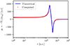 |
Fig. A.1. Static validation test: Radial profile of the gravitational field along (θ, φ) = (π/2, 0). The radius is in log scale. The grid configuration and boundary conditions are the same as our fiducial run, but we halved the resolution on each axis, uniformely for each patch. The density distribution is a uniform off-centered sphere of radius 1000, located at (r, θ, φ) = (3000, π/2, 0). We set |

We took the same grid configuration and boundary conditions as our fiducial run. We halved the resolution on each axis, uniformely for each patch, in order to reduce the computation time while keeping the grid anisotropy. The density distribution is uniform inside an off-centered sphere of radius 1000 au. The center is located at (r, θ, φ) = (3000, π/2, 0). We emphasize that only the self-gravity solver is tested here. Thus, as the physics is unimportant, we set  and G ≡ 1, and the quantities are displayed in code units. We set the convergence threshold to 10−5.
The theoretical and computed solutions are well matching thanks to the high resolution and low convergence threshold. The convergence rate for this test is about 600 iterations, starting from a zero initial guess potential. After this first "burn-in" computation, the solver requires between 1 and ∼102 iterations to converge, depending on the dynamics of the gas (it is 10 on average for our fiducial run). We checked that the scheme is second-order accurate for the gravitational potential (see Fig. A.2).
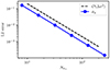 |
Fig. A.2. Convergence rate of the gravitational potential (dotted blue line) as a function of the grid spatial resolution using the BICGSTAB method. It is based on the off-centered sphere test. It exhibits second order spatial convergence. |
Figure A.3 shows the amplitude of density fluctuations in log scale as a function of time following Jean’s instability with the Poisson equation solved every timestep. Both quantities are adimensionned by background density ρ0 and cs0/L respectively, L = 10 u.c. being the domain size.
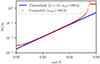 |
Fig. A.3. Dynamic validation test: Amplitude of density fluctuations in log scale as a function of time following Jean’s instability for λJ = 1/3 where Poisson equation is solved at every timestep. All quantities are dimensionless. The blue line is the theoretical prediction for the most unstable mode (λ = 10 u.c.), the red line is the computed result. |
The setup is 1D cartesian with periodic boundary conditions. The x coordinate is meshed with 1000 uniform cells and ranges between 0 and L. The density distribution is initialized with a Gaussian perturbation of amplitude 10−4. Setup is adiabatic with γ = 5/3, background density and pressure are ρ0 = 3, P0 = 1/γ in code units which gives λJ = 1/3 (G ≡ π).
For a given wavelength λ, the expected growth rate is given by  with λ > λJ. The mode of the largest wavelength is therefore the most unstable. Then, for λ = L, the theoretical growth rate is sth = 188.4 cs/L, and the associated perturbation should dominate the evolution of density perturbation.
This is confirmed by red dots, associated with the computed evolution of density perturbation, which matches the theoretical linear prediction for the most unstable mode (blue solid line) where cs0t/L is in the range 0.1 − 0.4. A linear regression in this portion of the slope gives scpt = 186.6 corresponding to a relative error of 0.9%. Hence, the dynamic is properly captured by our self-gravity solver.
Appendix B: Gravity step
The gravity calculation is performed just before the dynamical step. It triggers the gravitational potential computation from various sources. In our case, that includes self-gravity (see Appendix A) and point mass contribution.
In order to properly account for the whole gravitational feedback, the missing inner seed is assimilated to a point mass with:
 (B.1)
(B.1)
where Mpm and ϕpm are respectively the mass and associated potential of the point mass.
The initial mass is the one enclosed in a uniform sphere of radius rin and density ρ0. We sum up mass fluxes over the inner shell during the integration to update the central mass according to mass transits. The net gravitational potential used for the dynamical integration is then ϕg = ϕpm + ϕsg.
One can specify the frequency of the gravity step. Béthune & Rafikov (2019) showed that updating the gravitational potential every 4 dynamical timestep does not substantially impact the system evolution (see their test on Jeans’ instability).
We conducted our own test and obtained a relative error of 8% on the growth rate of the most unstable mode when computing gravity every 4 dynamical timestep. We consider this variation acceptable and choose to compute gravity every 4 timestep in our simulation to speed up the integration.
Appendix C: Chemical network
The magnetic diffusivities depend on the abundances of the charge carriers. To compute these abundances, we consider a simple chemical network based on Umebayashi & Nakano (1990) and Kunz & Mouschovias (2009). The network includes the following reactions:
 (C.1)
(C.1)
 (C.2)
(C.2)
 (C.3)
(C.3)
 (C.4)
(C.4)
 (C.5)
(C.5)
 (C.6)
(C.6)
 (C.7)
(C.7)
 (C.8)
(C.8)
 (C.9)
(C.9)
 (C.10)
 (C.11)
 (C.12)
 (C.13)
The ionization of H2 (Eq. C.1) is solely due to cosmic rays. We neglect shielding and focussing effects of cosmic rays, so the ionization rate ζ = 1.3 × 10⁻¹⁷ s−1 is assumed to be constant. The reaction rates for the ion-neutral (Eqs. C.2, C.3 and C.4), the dissociative recombination (Eq. C.5), and the radiative recombination (Eq. C.6) reactions are given by:
 (C.14)
where T is the temperature and α and β are the prefactor and temperature exponent, respectively. The values of α and β for each reaction are given in Table C.1.
Rate coefficients for the ion-neutral, dissociative recombination and radiative recombination reactions.
The reaction rates for electron attachment (Eq. C.7) and charge exchange reactions on neutral grains (Eqs. C.9 and C.11) are given by:
![Mathematical equation: $$ \begin{aligned} k = \pi a^2 {\left( \frac{8 k_B T}{\pi m} \right)}^{1/2} \left[ 1 + {\left( \frac{\pi e^2}{2 a k_B T} \right)}^{1/2} \right] S, \end{aligned} $$](/articles/aa/full_html/2024/06/aa48405-23/aa48405-23-eq57.gif) (C.15)
(C.15)
where a is the grain radius, kB is the Boltzmann constant, m is the mass of the electron or the ion, e is the electron charge, and S is a sticking coefficient, assumed to be 0.6 for electrons and 1 for ions, respectively. For electron attachement (Eq. C.8) and charge exchange reactions on charged grains (Eqs. C.10 and C.12), the reaction rates become:
![Mathematical equation: $$ \begin{aligned} k = \pi a^2 {\left( \frac{8 k_B T}{\pi m} \right)}^{1/2} \left( 1 + \frac{e^2}{a k_B T} \right) \left[ 1 + {\left( \frac{2}{2 + \left( a k_B T / e^2 \right)} \right)}^{1/2} \right] S, \end{aligned} $$](/articles/aa/full_html/2024/06/aa48405-23/aa48405-23-eq58.gif) (C.16)
(C.16)
We assume that grains are spherical with a radius a = 0.1 μm. The gas-to-dust mass ratio is assumed to be equal to 100. Assuming that the grains have a mass density of 3 g cm−3, this gives a grain abundance with respect to H nuclei of 1.3 × 10⁻¹².
Finally, we assume the following reaction rate for the H2 on grains (Eq. C.13):
 (C.17)
with α = 4.95 × 10⁻¹⁷ s−1.
Table C.2 gives the initial abundances. We assume that all hydrogen is in molecular form and that all carbon is in the form of CO. Iron is assumed to be ionized, so it has the same initial abundance as free electrons. Grains are assumed to be initially neutral. The abundances of all species in the chemical network are computed as a function of time using ASTROCHEM (Maret & Bergin 2015), until the steady-state equilibrium is reached.
Initial abundances with respect to H nuclei of the species considered in chemical network.
Fig. C.1 shows the abundances of the main charge carriers at the steady-state and the ionization fraction (that is the total abundance of positively or negatively charged species with respect to H nuclei), as function of the H number density, for a grain radius of a = 0.1 μm and a gas temperature given by Eq. (8). The abundances of the main charge carriers are in agreement with Umebayashi & Nakano (1990, see their Fig. 2, which corresponds to the same grain size and the similar initial abundances that those adopted here). The ionization fraction decreases with the density for nH < 1011 cm−3 and remains constant at higher densities. For densities lower than 1011 cm−3, the main charge carriers are free electrons and Fe+ ions. At higher densities, the main charge carriers are positively and negatively charged grains. The transition between the two regimes occurs when the ion fraction becomes comparable to the number density of grains.
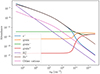 |
Fig. C.1. Abundances of the charge carriers at the steady-state as a function of the H number density for a = 0.1 μm and ζ = 1.3 × 10⁻¹⁷ s−1. The black dotted line shows the ionization fraction. |
Fig. C.2 shows the corresponding magnetic diffusivities (see Eqs. 3.4, 3.5 and 3.6 in Lesur 2021a) as a function of the H number density, for a magnetic field intensity B = 0.1(nH/cm−3)0.5 μG. The diffusivities are in agreement with Xu & Kunz (2021a, see their Fig. C2).
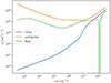 |
Fig. C.2. Magnetic diffusivities as a function of the H number density for a = 0.1 μm, ζ = 1.3 × 10⁻¹⁷ s−1, and B = 0.1(nH/cm−3)0.5 μG. The dashed line corresponds to a negative diffusivities. |
Appendix D: Internal boundaries
We use three internal boundaries in order to prevent a dramatic drop of the timestep without significant loss of accuracy: an Alvén speed limiter, diffusivity caps, and an advection timestep limiter.
In code units, Alvén speed is defined by
 (D.1)
(D.1)
where  .
.
Consequently, in strongly magnetized, low-density regions it can become very high and require very low timesteps, incompatible with the large timescale integration.
To alleviate this problem we introduce an Alvén speed limiter: for any cell of radius r if VA > VA, maxr the density is replaced with  . The associated velocities are updated following ui, new = ui ⋅ ρ/ρnew to satisfy as much as possible momentum conservation. Only uφ is left untouched. In this simulation, we set VA, max to 1 in code units.
Figure D.1, the top panel presents the Alvén speed profile at φ = 0 in the midplane (solid lines) and near the pole (dashed lines) for snapshots of increasing time. In the midplane, except for the very beginning, the Alvén speed limiter is never triggered. This is not the case near the pole. Because of cavity carving, the areas above and below the seed are strongly magnetized with low density and we need to limit the Alvén speed up to 100 au. That being said, the cavity region is barely discussed in this work because it is poorly described in the actual framework.
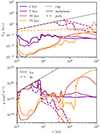 |
Fig. D.1. Top: Alvén speed in code units versus the radius, where φ = 0. Solid lines are the midplane values (θ ≈ π/2) while dashed lines are closer to the pole (θ ≈ π/3). The lighter the color, the later the snapshot. The dotted black line is the Alvén cap VA = VA, maxr where VA, max = 1 u.c.. Bottom: Ambipolar (solid) and Ohmic (dashed) diffusions versus the radius. Color coding and dotted black line are the same as for the top panel, with the diffusivity cap η = η0r2 where η0 ≈ 7.1 × 1018 cm2 s−1. |
We also use diffusivity caps following Xu & Kunz (2021a,b). The timestep associated with diffusion processes is proportional to Δl2/η, where Δl is the typical cell size and η is the diffusivity coefficient associated with the diffusion process. Particularly strong values of ηA and η0 are therefore susceptible to dramatically slow down the integration.
We solve the problem by introducing a diffusivity cap such that for any cell of radius r, if ηA, O > η0r2, the diffusivity coefficient is replaced with ηA, O = η0r2. Here, η0 ≈ 7.1 × 1018 cm2 s−1 is the conversion factor from code units to physical units.
Figure D.1, bottom panel shows the ambipolar (solid lines) and Ohmic (dashed lines) diffusivity profiles at φ = 0 for the same snapshots as the top panel. The cap is triggered for ambipolar diffusion only in the very beginning. Ohmic diffusion, however, is limited for radii below 5 au as soon as the disk forms and remains so until the end. This is expected as Ohmic diffusion increases with gas density.
The last internal boundary, the advection timestep limiter, is a consequence of the first one. In the innermost regions, gas affected by the Alvén limiter cannot be launched in the outflow. Conversely, it is falling back onto the seed, reaching high velocities that limit the timestep. To solve this problem, we use a timestep limiter such that where dtadv < dtmin, the velocity components are updated following ui, new = ui ⋅ dtmin/dtadv. We set dtmin = 1 u.c.
We monitored the total mass and angular momentum in the system during the integration to ensure that none of these routines was significantly affecting their balance.
All Tables
Rate coefficients for the ion-neutral, dissociative recombination and radiative recombination reactions.
Initial abundances with respect to H nuclei of the species considered in chemical network.
All Figures
|
Fig. 1. Snapshots of the azimuthally averaged particle density (color) with attached poloidal magnetic field lines (white contours) and poloidal velocity stream (gray arrows). From left to right, the first snapshot is a large-scale view focusing on the cloud morphology significantly before the first core formation, while the three last snapshots zoom into the first core during and after its formation. |
| In the text | |
|
Fig. 2. Azimuthally averaged surface density (top left), rotation rate (top right), poloidal magnetic field intensity (bottom left), and plasma parameter βP (bottom right) versus the radius, computed in the midplane. Each color corresponds to one snapshot, the darker being the disk formation epoch, while the lighter is associated with the later times of the simulation. In the top right panel, the dashed black line is the theoretical Keplerian rotation rate with M⋆ ≈ 0.7 M⊙. |
| In the text | |
|
Fig. 3. Gas surface density in the equatorial plane. From left to right: three characteristic snapshots illustrating the successive behaviors of the disk at 5, 30, and 70 kyr respectively. |
| In the text | |
|
Fig. 4. Top panel: radius of the disk over time. The dash-dotted black lines emphasize the radii where the mass accretion rate is inspected in the next panel. Middle panel: mass accretion rate over time near the protostar (R = 5 au, red) and at the maximum stable outer radius (R = 60 au, green). Dashed lines correspond to expanding material. Bottom panel: protostar mass (orange), disk mass (blue), the total mass of the disk-protostar system (gray), and envelope mass (brown) over time. Data for the accretion rate are convolved in time using a 10 kyr window (equivalent to 8 orbits at 100 au). |
| In the text | |
|
Fig. 5. From top to bottom we focus on t = 5, 30 and 70 kyr respectively. Each panel presents GRφ (green), MZφ (blue) and HZφ (red) versus the radius. Solid and dashed lines are associated with positive and negative stresses respectively. The dotted black line is the corresponding disk radius. Data are convolved in time using a 10 kyr window (equivalent to 8 orbits at 100 au). |
| In the text | |
|
Fig. 6. Mass accretion rate versus the radius. Each color corresponds to one snaphsot at 5, 30 and 70 kyr respectively. The lighter, the later. Dashed lines represent the disk radius associated with each epoch. Data are convolved in time using a 10 kyr window (equivalent to 8 orbits at 100 au). |
| In the text | |
|
Fig. 7. Spacetime diagrams of the surface density (top panel), poloidal magnetic flux (middle panel), and Toomre parameter (bottom panel). Colors and radii are in log scale. The dashed white line corresponds to the disk radius, and dash-dotted white lines delimit the three accretion phases. Data were convolved in time using a 10 kyr window (equivalent to 8 orbits at 100 au). |
| In the text | |
|
Fig. 8. From left to right we focus on t = 5, 30, and 70 kyr respectively, corresponding to each accretion phase. Each panel presents the specific angular momentum j in colors, with the attached poloidal velocity flow Vp as white quivers. |
| In the text | |
|
Fig. 9. Ideal magnetic flux velocity transport versus the radius. Each color corresponds to one snapshot at 5, 30, and 70 kyr respectively. The lighter, the later. Dashed lines represent the disk radius associated with each epoch. Data are convolved in time using a 10 kyr window (equivalent to 8 orbits at 100 au). |
| In the text | |
|
Fig. 10. disk surface density versus the radius. Each color focuses on one accretion phase at 5, 30, and 70 kyr respectively. The lighter, the later. The dashed black line is the predicted critical surface density from Eq. (19). |
| In the text | |
|
Fig. 11. Top row: large-scale equatorial slice of the gas surface density with associated equatorial velocity flow (white quivers). A dashed white line indicates the azimuth of the main streamer, for which poloidal slices are performed. Middle row: large-scale poloidal slice of the gas particle density with associated poloidal velocity flow (white quivers). Bottom row: large-scale poloidal slice of the gas poloidal velocity, normalized by the free-fall velocity, with associated poloidal velocity flow (white quivers). Each column corresponds to a late time snapshot, respectively at 60 (left column) and 70 kyr (right column). In each plot, a line integrated convolution treatment is applied to emphasize the gas streamlines. The innermost 100 au are masked by a gray circle to allow for adequate contrast. |
| In the text | |
|
Fig. 12. Large-scale equatorial slice at t = 60 kyr. Colors are the plasma parameter βP. |
| In the text | |
|
Fig. 13. Three-dimensional representation of the disk and streamer with two attached streamlines at time 70 kyr. Red surfaces correspond to the disk, while green surfaces represent the streamer. Both streamlines start at R = 350 au and φ = φstreamer with respectively Z = 0 (orange solid line) and Z = 100 au (blue solid line). Black dots indicate shocks (or rarefactions) along the streamlines while the gray dot corresponds to a density transition (see Fig. 14 for their identification). For an animated version of the figure with a large-scale visualization of the streamer, see https://cloud.univ-grenoble-alpes.fr/s/ZNwHrbWg8A24Trb. |
| In the text | |
|
Fig. 14. Top: particle density along the streamlines starting at Z0 = 0 au and Z0 = 100 au respectively. Bottom: Gas velocity projected along each streamline. Colors and dots are the same as in Fig. 13. |
| In the text | |
|
Fig. A.1. Static validation test: Radial profile of the gravitational field along (θ, φ) = (π/2, 0). The radius is in log scale. The grid configuration and boundary conditions are the same as our fiducial run, but we halved the resolution on each axis, uniformely for each patch. The density distribution is a uniform off-centered sphere of radius 1000, located at (r, θ, φ) = (3000, π/2, 0). We set |
| In the text | |
|
Fig. A.2. Convergence rate of the gravitational potential (dotted blue line) as a function of the grid spatial resolution using the BICGSTAB method. It is based on the off-centered sphere test. It exhibits second order spatial convergence. |
| In the text | |
|
Fig. A.3. Dynamic validation test: Amplitude of density fluctuations in log scale as a function of time following Jean’s instability for λJ = 1/3 where Poisson equation is solved at every timestep. All quantities are dimensionless. The blue line is the theoretical prediction for the most unstable mode (λ = 10 u.c.), the red line is the computed result. |
| In the text | |
|
Fig. C.1. Abundances of the charge carriers at the steady-state as a function of the H number density for a = 0.1 μm and ζ = 1.3 × 10⁻¹⁷ s−1. The black dotted line shows the ionization fraction. |
| In the text | |
|
Fig. C.2. Magnetic diffusivities as a function of the H number density for a = 0.1 μm, ζ = 1.3 × 10⁻¹⁷ s−1, and B = 0.1(nH/cm−3)0.5 μG. The dashed line corresponds to a negative diffusivities. |
| In the text | |
|
Fig. D.1. Top: Alvén speed in code units versus the radius, where φ = 0. Solid lines are the midplane values (θ ≈ π/2) while dashed lines are closer to the pole (θ ≈ π/3). The lighter the color, the later the snapshot. The dotted black line is the Alvén cap VA = VA, maxr where VA, max = 1 u.c.. Bottom: Ambipolar (solid) and Ohmic (dashed) diffusions versus the radius. Color coding and dotted black line are the same as for the top panel, with the diffusivity cap η = η0r2 where η0 ≈ 7.1 × 1018 cm2 s−1. |
| In the text | |
Current usage metrics show cumulative count of Article Views (full-text article views including HTML views, PDF and ePub downloads, according to the available data) and Abstracts Views on Vision4Press platform.
Data correspond to usage on the plateform after 2015. The current usage metrics is available 48-96 hours after online publication and is updated daily on week days.
Initial download of the metrics may take a while.