| Issue |
A&A
Volume 686, June 2024
|
|
|---|---|---|
| Article Number | A282 | |
| Number of page(s) | 16 | |
| Section | Planets and planetary systems | |
| DOI | https://doi.org/10.1051/0004-6361/202347759 | |
| Published online | 21 June 2024 | |
Precise characterisation of HD 15337 with CHEOPS: A laboratory for planet formation and evolution★,★★,★★★
1
Instituto de Astrofisica e Ciencias do Espaco, Universidade do Porto, CAUP,
Rua das Estrelas,
4150-762
Porto,
Portugal
e-mail: This email address is being protected from spambots. You need JavaScript enabled to view it.
2
Departamento de Fisica e Astronomia, Faculdade de Ciencias, Universidade do Porto,
Rua do Campo Alegre,
4169-007
Porto,
Portugal
3
Dipartimento di Fisica, Università degli Studi di Torino,
Via Pietro Giuria 1,
10125,
Torino,
Italy
4
Physikalisches Institut, University of Bern,
Gesellschaftsstrasse 6,
3012
Bern,
Switzerland
5
Center for Space and Habitability, University of Bern,
Gesellschaftsstrasse 6,
3012
Bern,
Switzerland
6
Department of Physics and Kavli Institute for Astrophysics and Space Research, Massachusetts Institute of Technology,
Cambridge,
MA
02139,
USA
7
Observatoire Astronomique de l'Université de Genève,
Chemin Pegasi 51,
1290
Versoix,
Switzerland
8
Department of Astronomy, Stockholm University, AlbaNova University Center,
10691
Stockholm,
Sweden
9
Aix-Marseille Univ., CNRS, CNES, LAM,
38 rue Frédéric Joliot-Curie,
13388
Marseille,
France
10
Division Technique INSU,
CS20330,
83507 La
Seyne-sur-Mer cedex,
France
11
Centre for Exoplanet Science, SUPA School of Physics and Astronomy, University of St Andrews,
North Haugh,
St Andrews
KY16 9SS,
UK
12
Space Research Institute, Austrian Academy of Sciences,
Schmiedl-strasse 6,
A-8042
Graz,
Austria
13
Cavendish Laboratory,
JJ Thomson Avenue,
Cambridge
CB3 0HE,
UK
14
Astrobiology Research Unit, Université de Liège,
Allée du 6 Août 19C,
4000
Liège,
Belgium
15
Space sciences, Technologies and Astrophysics Research (STAR) Institute, Université de Liège,
Allée du 6 Août 19C,
4000
Liège,
Belgium
16
Instituto de Astrofisica de Canarias,
Via Lactea s/n,
38200 La
Laguna,
Tenerife,
Spain
17
Departamento de Astrofisica, Universidad de La Laguna,
Astrofísico Francisco Sanchez s/n,
38206 La
Laguna,
Tenerife,
Spain
18
Institut de Ciencies de l’Espai (ICE, CSIC),
Campus UAB, Can Magrans s/n,
08193
Bellaterra,
Spain
19
Institut d’Estudis Espacials de Catalunya (IEEC),
Gran Capità 2-4,
08034
Barcelona,
Spain
20
European Space Agency (ESA), European Space Research and Technology Centre (ESTEC),
Keplerlaan 1,
2201 AZ
Noordwijk,
The Netherlands
21
Admatis,
5. Kandó Kálmán Street,
3534
Miskolc,
Hungary
22
Depto. de Astrofisica, Centro de Astrobiologia (CSIC-INTA),
ESAC campus,
28692
Villanueva de la Cañada (Madrid),
Spain
23
Sub-department of Astrophysics, Department of Physics, University of Oxford,
Oxford
OX1 3RH,
UK
24
Max Planck Institut für Extraterrestrische Physik,
Gießenbachstraße 1,
85748
Garching bei München,
Germany
25
INAF, Osservatorio Astronomico di Padova,
Vicolo dell’Osservatorio 5,
35122
Padova,
Italy
26
Université Grenoble Alpes, CNRS, IPAG,
38000
Grenoble,
France
27
Université de Paris Cité, Institut de physique du globe de Paris, CNRS,
1 rue Jussieu,
75005
Paris,
France
28
Institute of Planetary Research, German Aerospace Center (DLR),
Rutherfordstrasse 2,
12489
Berlin,
Germany
29
INAF, Osservatorio Astrofisico di Torino,
Via Osservatorio, 20,
10025
Pino Torinese To,
Italy
30
Centre for Mathematical Sciences, Lund University,
Box 118,
221 00
Lund,
Sweden
31
Centre Vie dans l’Univers, Faculté des sciences, Université de Genève,
Quai Ernest-Ansermet 30,
1211
Genève 4,
Switzerland
32
Thüringer Landessternwarte Tautenburg,
Sternwarte 5,
07778
Tautenburg,
Germany
33
Leiden Observatory, University of Leiden,
PO Box 9513,
2300 RA
Leiden,
The Netherlands
34
Department of Space, Earth and Environment, Chalmers University of Technology,
Onsala Space Observatory,
439 92
Onsala,
Sweden
35
Department of Astrophysics, University of Vienna,
Türkenschanzs-trasse 17,
1180
Vienna,
Austria
36
Konkoly Observatory, Research Centre for Astronomy and Earth Sciences,
1121
Budapest,
Konkoly Thege Miklós út 15–17,
Hungary
37
ELTE Eötvös Loránd University, Institute of Physics,
Pázmány Péter sétány 1/A,
1117
Budapest,
Hungary
38
IMCCE, UMR8028 CNRS, Observatoire de Paris, PSL Univ., Sorbonne Univ.,
77 av. Denfert-Rochereau,
75014
Paris,
France
39
Institut d’astrophysique de Paris, UMR7095 CNRS, Université Pierre & Marie Curie,
98bis blvd. Arago,
75014
Paris,
France
40
Astrophysics Group, Lennard Jones Building, Keele University,
Staffordshire
ST5 5BG,
UK
41
European Southern Observatory,
Karl-Schwarzschild-Straße 2,
Garching bei München
85748,
Germany
42
Mullard Space Science Laboratory, University College London,
Holmbury St. Mary, Dorking,
Surrey
RH5 6NT,
UK
43
INAF, Osservatorio Astrofisico di Catania,
Via S. Sofia 78,
95123
Catania,
Italy
44
Institute of Optical Sensor Systems, German Aerospace Center (DLR),
Rutherfordstrasse 2,
12489
Berlin,
Germany
45
Dipartimento di Fisica e Astronomia “Galileo Galilei”, Università degli Studi di Padova,
Vicolo dell’Osservatorio 3,
35122
Padova,
Italy
46
Department of Physics, University of Warwick,
Gibbet Hill Road,
Coventry
CV4 7AL,
UK
47
ETH Zurich, Department of Physics,
Wolfgang-Pauli-Strasse 2,
8093
Zurich,
Switzerland
48
Zentrum für Astronomie und Astrophysik, Technische Universität Berlin,
Hardenbergstr. 36,
10623
Berlin,
Germany
49
Institut für Geologische Wissenschaften, Freie Universität Berlin,
Maltheserstrasse 74–100,
12249
Berlin,
Germany
50
ELTE Eötvös Loránd University, Gothard Astrophysical Observatory,
9700
Szombathely,
Szent Imre h. u. 112,
Hungary
51
HUN-REN-ELTE Exoplanet Research Group,
9700
Szombathely,
Szent Imre h. u. 112,
Hungary
52
Institute of Astronomy, University of Cambridge,
Madingley Road,
Cambridge
CB3 0HA,
UK
Received:
18
August
2023
Accepted:
22
March
2024
Abstract
Context. The HD 15337 (TIC 120896927, TOI-402) system was observed by the Transiting Exoplanet Survey Satellite (TESS), revealing the presence of two short-period planets situated on opposite sides of the radius gap. This offers an excellent opportunity to study theories of formation and evolution, as well as to investigate internal composition and atmospheric evaporation.
Aims. We aim to constrain the internal structure and composition of two short-period planets situated on opposite sides of the radius valley: HD 15337 b and c. We use new transit photometry and radial velocity data.
Methods. We acquired 6 new transit visits with the CHaracterising ExOPlanet Satellite (CHEOPS) and 32 new radial velocity measurements from the High Accuracy Radial Velocity Planet Searcher (HARPS) to improve the accuracy of the mass and radius estimates for both planets. We re-analysed the light curves from TESS sectors 3 and 4 and analysed new data from sector 30, correcting for long-term stellar activity. Subsequently, we performed a joint fit of the TESS and CHEOPS light curves, along with all available RV data from HARPS and the Planet Finder Spectrograph (PFS). Our model fit the planetary signals, stellar activity signal, and instrumental decorrelation model for the CHEOPS data simultaneously. The stellar activity was modelled using a Gaussian-process regression on both the RV and activity indicators. Finally, we employed a Bayesian retrieval code to determine the internal composition and structure of the planets.
Results. We derived updated and highly precise parameters for the HD 15337 system. Our improved precision on the planetary parameters makes HD 15337 b one of the most precisely characterised rocky exoplanets, with radius and mass measurements achieving a precision better than 2% and 7%, respectively. We were able to improve the precision of the radius measurement of HD 15337 c to 3%. Our results imply that the composition of HD 15337 b is predominantly rocky, while HD 15337 c exhibits a gas envelope with a mass of at least 0.01 M⊕.
Conclusions. Our results lay the groundwork for future studies, which can further unravel the atmospheric evolution of these exoplanets and offer new insights into their composition and formation history as well as the causes behind the radius gap.
Key words: techniques: photometric / techniques: radial velocities / planets and satellites: composition / stars: individual: HD 15337 / stars: individual: TOI-402 / stars: individual: TIC 12089692
The data are available at the CDS via anonymous ftp to cdsarc.cds.unistra.fr (130.79.128.5) or via https://cdsarc.cds.unistra.fr/viz-bin/cat/J/A+A/686/A282
This article uses data from CHEOPS programme CH_PR100031.
Based on observations made with ESO-3.6 m telescope at the La Silla Observatory under programme ID 1102.C-0923.
© The Authors 2024
 Open Access article, published by EDP Sciences, under the terms of the Creative Commons Attribution License (https://creativecommons.org/licenses/by/4.0), which permits unrestricted use, distribution, and reproduction in any medium, provided the original work is properly cited.
This article is published in open access under the Subscribe to Open model. This email address is being protected from spambots. You need JavaScript enabled to view it. to support open access publication.
1 Introduction
The search for exoplanets orbiting solar-type stars has led to a large increase in the number of known planets in recent years. Space missions such as Kepler (Borucki 2016) and the Transiting Exoplanet Survey Satellite (TESS; Ricker et al. 2014) have been directly responsible for this rise, leading to the detection of many multi-planet systems that are composed of planets in the super-Earth (Rp = 1–2 R⊙) and sub-Neptune (Rp = 2–4 R⊙) regimes. Multi-planet systems that contain two or more small planets with similar masses are of particular importance to understand the formation and evolution of exoplanetary systems and even our own Solar System, by studying the differences in structure and composition between each planet. In some systems (e.g. HD 3167, Gandolfi et al. 2017; HD 23472, Barros et al. 2022), the planets lie on opposite sides of the radius gap (Fulton et al. 2017), which is defined as a gap in the radius distribution where not many planets have been detected. Some possible explanations for this apparent gap include the effect of atmospheric photoevap-oration (e.g. Owen & Wu 2017; Venturini et al. 2020), gas-poor formation (e.g. Lee & Chiang 2016), or giant impact erosion (e.g. Liu et al. 2015). Atmospheric evaporation is the most accepted explanation for this gap. Since the presence of a gas envelope is enough to significantly change the radius of a planet while maintaining a similar mass, it is possible that the smaller planets lost their envelopes due to stellar irradiation. However, Luque & Pallé (2022) have suggested the gap is not a radius gap, but a density gap, and that orbital migration of water-rich worlds can explain the observations and the population of sub-Neptunes.
The CHaracterising ExOPlanet Satellite (CHEOPS; Benz et al. 2021) is an ESA space telescope designed as a follow-up mission aiming at the precise characterisation of exoplane-tary systems around nearby bright stars. It was launched on December 18, 2019 and has been orbiting at ~700 km above Earth since then. The increased precision in the photometry measurements makes CHEOPS observations a valuable addition to previously obtained transiting light curves (from TESS or ground-based observatories), which leads to a highly precise radius and an improvement in the internal characterisation of the planets.
HD 15337 (TIC 120896927, TOI-402) is a bright (V = 9) K1 dwarf, known to host two planets lying on opposite sides of the radius valley (Gandolfi et al. 2019; Dumusque et al. 2019), which were first detected using TESS observations and confirmed with HARPS radial velocity (RV) measurements. HD 15337 b is a short-period (P = 4.76 d) super-Earth with R = 1.78R⊕ and M = 6.5 M⊕ with a companion sub-Neptune (HD 15337 c) with a 17.2-day period and a similar mass (M = 6.7 M⊕) but a larger radius (R = 2.5 R⊕), thought to have a gaseous envelope. As such, it is one of the most amenable systems to study the physics behind the radius valley due to the characteristics of both planets and the brightness of the star.
In this paper, we use archive and new TESS data and newly obtained CHEOPS photometric observations, together with archive and new ground-based RV measurements from HARPS and the Planet Finder Spectrograph (PFS), to improve the precision of the radius and the mass of HD 15337 b and HD 15337 c. We present a summary of the observations and data reduction methods in Sect. 2, followed by the estimation of the stellar parameters in Sect. 3. In Sect. 4, we describe our models and assumptions and summarise the new results. We discuss our results in Sect. 5 and conclude with a short summary of our findings in Sect. 6.
2 Observations
2.1 CHEOPS
We obtained six CHEOPS visits of HD 15337 as part of the CHEOPS Guaranteed Time Observation (GTO) programme, for a total observation time of ~2.2 days. We obtained three transits of planet b and 2 transits of planet c, plus an overlapping transit of both planets during the first visit. The details of each visit are summarised in the observation log in Table 1.
The data of each visit were reduced with the CHEOPS data reduction pipeline1 (DRP; Hoyer et al. 2020), which processes all the data automatically and corrects for bias, gain, dark, flat, and environmental effects such as cosmic ray impacts, background, and smearing. The DRP extracts the photometric signal in four apertures, RINF, DEFAULT, RSUP, and OPTIMAL, which calculates the optimal radius based on maximising the signal-to-noise ratio (S/N) of the light curve. It then produces a file with all the extracted light curves and additional data such as the roll angle time series, quality flags, and the background time series used for the corrections. We chose the DEFAULT setting, with a radius of 25 pix, that was considered to be the best according to the data reduction report.
2.2 TESS
HD 15337 was previously observed by Camera #2 of TESS with a two-minute cadence in sector 3 (from 2018-Sep-20 to 2018-Oct-18) and sector 4 (2018-Oct-18 to 2018-Nov-15), as reported in Gandolfi et al. (2019) and Dumusque et al. (2019), and more recently in sector 30 (2020-Sep-22 to 2020-Oct-21) which we include in this analysis. A total of 13 transits of HD 15337 b and five of HD 15337 c were found in the three sectors.
The data were reduced by the Science Processing Operations Center (SPOC; Jenkins 2020) pipeline and the fits files were downloaded from the Mikulski Archive for Space Telescopes (MAST) portal2. In this analysis, we employed the Presearch Data Conditioning Simple Aperture Photometry (PDCSAP) light curves, which were corrected to remove instrumental sys-tematics, outliers, discontinuities, and other non-astrophysical long-term trends from the data (Smith et al. 2012, 2017).
The files obtained from the SPOC pipeline contain a quality parameter that identifies data points that have been impacted by abnormal occurrences including attitude changes, momentum dumps, and thruster firings (Tenenbaum & Jenkins 2018). To ensure the reliability of the data, we deleted all the bad-quality flagged data points from our light curve, as well as any NaN values present, before detrending and processing the data. We followed a similar approach to the one described in Rosário et al. (2022) for the correction of the TESS light curves. We isolated each individual transit, keeping all points within three transit durations of the estimated mid-transit time and removing the remaining out-of-transit data. We normalised each transit light curve separately to avoid the influence of long-term trends, using a low-order polynomial fit. We used the Bayesian inference criterion (BIC) to choose the order of the polynomial for each transit, with a linear trend being preferred in the majority of the cases.
2.3 HARPS
HD 15337 was Doppler-monitored between 15 December 2003 and 6 September 2017 UT using the HARPS spectrograph (R ≈ 115 000; Mayor et al. 2003) mounted at the ESO-3.6m telescope (La Silla Observatory; see Gandolfi et al. 2019; Dumusque et al. 2019). We retrieved the 87 publicly available data from the ESO archive and acquired 32 additional HARPS spectra between 9 July and 12 September 2019 UT, as part of our follow-up program of TESS transiting planets (ID: 1102.C-0923; PI: Gandolfi). We set the exposure time to Texp = 900–1800 s based on seeing and sky conditions, leading to a median S/N of ~92 per pixel at 550 nm. We reduced the archival and new HARPS data using the dedicated data reduction software (DRS; Lovis & Pepe 2007) and extracted the radial velocity (RV) measurements cross–correlating the Echelle spectra with a K5 numerical mask (Baranne et al. 1996; Pepe et al. 2002). We also used the DRS to extract the full-width half maximum (FWHM) and bisector inverse slope (BIS) of the cross-correlation function (CCF) and the Ca II H & K lines activity index3  . In June 2015, the HARPS spectrograph was upgraded by replacing the circular fibres with octagonal ones (Lo Curto et al. 2015). To account for the RV offset due to the instrument refurbishment, we treated the archive HARPS RV measurements taken before (52 measurements) and after (67 measurements) June 2015 as independent data sets.
The HARPS RVs were corrected for secular acceleration following the equations from Kuerster et al. (2003). We retrieved the stellar RV and proper motion from Gaia DR2 (Soubiran et al. 2018) and EDR3 (Gaia Collaboration 2020), respectively, and found the average secular acceleration during the HARPS observations time frame to be 0.05189 ms−1 yr−1. Given the 15.743 yr baseline of the HARPS data, the secular acceleration implies a correction up to about +0.82 ms−1 for the last data point in our time series.
CHEOPS observation log for HD 15337.
2.4 PFS
HD 15337 was observed as part of the Magellan-TESS Survey (MTS) published in Teske et al. (2021). The MTS followed up several pre-selected planets from TESS to obtain RVs using the Planet Finder Spectrograph (PFS; Crane et al. 2006, 2008, 2010) located on the Magellan II Clay telescope at the Las Campanas Observatory. PFS is a precision RV spectrograph commissioned in October 2009, used primarily for the search of new planets and follow-up transit planet candidates. The PFS detector (from January 2018) has a 10k × 10k CCD detector with 9 µm pixels and a resolving power of ~ 130 000. HD 15337 was observed between 12 February 2019 and 20 December 2019 and 48 new RV measurements were obtained. The spectra were reduced in Teske et al. (2021) using a custom pipeline based on the one from Butler et al. (1996). The PFS RVs were included as a separate dataset in our analysis to account for the different offset.
3 Stellar characterisation
The spectroscopic stellar parameters for HD 15337 (effective temperature, Teff, surface gravity, log g, microturbulence velocity, and iron content, [Fe/H]) were taken from a previous version of SWEET-Cat (Santos et al. 2013; Sousa et al. 2018). The parameters were estimated based on a combined HARPS spectrum with the ARES+MOOG methodology using the latest version of ARES4 (Sousa et al. 2007, 2015) to consistently measure the equivalent widths (EWs) of selected iron lines on the spectrum. In this analysis, we used a minimisation process to find the ionisation and excitation equilibrium to converge for the best set of spectroscopic parameters. This process makes use of a grid of Kurucz model atmospheres (Kurucz 1993) and the radiative transfer code MOOG (Sneden 1973). Since the star is cooler than 5200 K, we used the appropriate iron line list for our method presented in Tsantaki et al. (2013). More recently, the same methodology was applied on a more recent combined HARPS spectrum, where we derived new spectroscopic stellar parameters (Teff = 5088 ± 78 K, log g = 4.24 ± 0.10 (dex), and [Fe/H] 0.04 ± 0.03 dex; Sousa et al. 2021), consistent within 2.2σ. Here, we also derived a more accurate trigonometric surface gravity using recent Gaia DR3 data (Gaia Collaboration et al. 2016, 2023) following the same procedure as described in Sousa et al. (2021), which provided a consistent value when compared with the spectroscopic surface gravity (4.48 ± 0.04 dex). Abundances of magnesium (Mg) and silicon (Si) were also derived using the same tools and models as for the stellar parameter determination, as well as using the classical curve-of-growth analysis method assuming local thermodynamic equilibrium. For the derivation of the abundances, we closely followed the methods described in Adibekyan et al. (2012, 2015).
We determined the radius of HD 15337 using a Markov chain Monte Carlo (MCMC) modified infrared flux method (Blackwell & Shallis 1977; Schanche et al. 2020). This was done by building spectral energy distributions (SEDs) from stellar atmospheric models defined by our spectral analysis and calculating the stellar bolometric flux by comparing synthetic and observed broadband photometry in the following bandpasses: Gaia G, GBP, and GRP, 2MASS J, H, and K, and WISE W1 and W2 (Skrutskie et al. 2006; Wright et al. 2010; Gaia Collaboration 2021). Using the known physical relations, we thus obtained the stellar effective temperature and angular diameter that can be converted to a radius using the offset-corrected Gaia parallax (Lindegren et al. 2021). To correctly estimate the error in our stellar radius, we conducted a Bayesian modelling averaging of the ATLAS (Kurucz 1993; Castelli & Kurucz 2003) and PHOENIX (Allard 2014) catalogues to produce a weighted averaged posterior distribution of the radius that encapsulates uncertainties in stellar atmospheric modelling. From this analysis, we obtained Rs = 0.855 ± 0.008 R⊙.
We then derived the isochronal mass, Ms, and age, ts, by inputting Teff, [Fe/H], and Rs along with their uncertainties into two different stellar evolutionary models. Specifically, we computed a first pair of mass and age estimates (Ms,1 ± σM1, ts,1 ± σt1) through the isochrone placement algorithm (Bonfanti et al. 2015, 2016), which interpolates the input set within pre-computed grids of PARSEC5 vl.2S (Marigo et al. 2017) tracks and isochrones. Further providing Prot = 36.5 days (Gandolfi et al. 2019) to our interpolating routine, we coupled the isochrone fitting with the gyrochronological relation from Barnes (2010), which is implemented in our isochrone placement to improve the optimisation scheme convergence, as detailed in Bonfanti et al. (2016) and retrieve more precise stellar parameters (see e.g. Angus et al. 2019). A second pair (MS,2 ± σM2, ts,2 ± σt2) was derived using Code Liégeois d’Évolution Stellaire (CLES; Scuflaire et al. 2008), which generates the best-fit evolutionary track according to the input set of stellar parameters following the Levenberg–Marquadt minimisation scheme (see e.g. Salmon et al. 2021). We successfully checked the mutual consistency of the two respective pairs of outcomes via the χ2 -based criterion described in Bonfanti et al. (2021) and then we merged the two probability density functions inferred from both the two pairs (Ms,1 ± σM1, Ms,2 ± σM2) and (ts,1 ± σt1, ts,2 ± σt2); finally, we obtained Ms = 0.840 ± 0.041 M⊙ and  Gyr. We refer to Bonfanti et al. (2021) for further details about the statistical methodology we followed. The derived stellar parameters can be found in Table 2.
Finally, we note that HD 15337 has a very dim stellar companion (Δm ~ 9.33 mag at 832 nm, Lester et al. 2021), which has been detected via speckle imaging at an angular separation of 1.4″ from the primary (Ziegler et al. 2020; Lester et al. 2021). The inferred stellar mass ratio (mass of the secondary over the mass of the primary) is 0.14 (Lester et al. 2021). The presence of a blended stellar companion causes a dilution factor in the planetary radii; in cases where the planets orbit the primary star, this can be computed using Eq. (7) of Ciardi et al. (2015). Using that equation, we find a correction factor of 1.00009 (as long as the planets orbit the primary). For this particular system, it is rather straightforward to conclude that the planets orbit the primary. If one of the planets was orbiting the secondary, the maximum possible transit depth would correspond to a configuration where such a planet would completely block the flux stemming from the secondary star. This would yield a maximum transit depth in our light curves of δmax ~ 185 ppm6. The transit depth that we measure with CHEOPS for planet b is δ ≈ 364 ppm and δ ≈ 735 ppm for planet c. Thus, the transits are too deep to correspond to the secondary star and we can confidently conclude that the two planets orbit the primary. The correction factor for the planetary radii is sufficiently small for our interior characterisation analysis not to be affected by the small dilution effect caused by the stellar companion.
4 Data analysis
4.1 Detrending of CHEOPS light curves
The light curves shown in Fig. 1 show strong correlations with the roll angle as well as other systematic effects. CHEOPS is located in a nadir-locked low-Earth orbit, which means the field stars rotate around the target star as a function of the position of the spacecraft in its orbit. This also leads to a correlation between the background flux and the roll angle, especially when approaching an Earth occultation. The gaps in the observations can be caused by Earth occultations due to the CHEOPS orbit placement or by South Atlantic Anomaly (SAA) crossings.
Another relevant effect for the majority of the targets observed by CHEOPS is temperature variation. Temperature perturbations are caused mainly by Earth occultations or when moving between targets due to the position of CHEOPS relative to the sun. This causes a ramp effect at the beginning of each time series that is discussed in more detail in Morris et al. (2021) and is corrected by detrending against the temperature of the telescope tube using the ThermFront2 Sensor temperature parameter included in the CHEOPS light curves.
We first removed outliers by performing a sigma-clip at 3σ using the centroid X and Y time series and at 6σ in the flux, ensuring we did not remove any part of the transit. The centroid position can be affected by cosmic rays, stray light or satellite trails crossing the point spread function, which helps to identify outliers. Points that varied more than 10% from the background-flux time series were also removed.
To mitigate the impact of these instrumental variations on the light curve, we performed a spline decorrelation simultaneously to the transit model fitting with the code LISA (Demangeon et al. 2018, 2021). The spline decorrelation consists of a sequential fit of the residuals against the time series of the roll angle, cen-troid position, temperature of the telescope tube, and measured background.
Overview of fundamental stellar parameters for HD 15337.
4.2 Radial velocity periodogram analysis
Figure 2 shows the offset-corrected radial velocity (RV) time series from HARPS and PFS, as well as several activity indicators obtained from the HARPS data reduction: FWHM, BIS and  . The generalised Lomb Scargle (GLS; Zechmeister & Kürster 2009) periodogram of each of the aforementioned time series is plotted alongside. A long-term trend is visible in the plotted RVs, which could be caused by long-term stellar activity like a magnetic cycle. The presence of a similar trend in the FWHM time series further hints towards a signal induced by activity. The Pearson correlation factors obtained between the RV and the FWHM series show a strong linear correlation (p-value of 5 × 10⁻⁷). However, there appears to be no long-term linear correlation (p-value of 0.25) with the
  series. The main peak in the RV time series clearly shows the presence of a planetary signal around the period of HD 15337 b reported by Gandolfi et al. (2019) and Dumusque et al. (2019), which is not present in any of the indicators. We do not see, at first glance, an indication of any significant peak near the period of HD 15337 c. To verify its presence, we removed the Doppler signal of the planet by modelling it as a Keplerian with the radvel package, fixing period and phase at the transit ephemerides. Figure 3 shows the periodogram of the RV residuals after removing planet b (in the middle-lower panel) and both planets b and c (in the lower panel). For this preliminary analysis we removed the long-term trends that are shown in the first plot of Fig. 2 by fitting a simple second-degree polynomial. We see that removing the trends and the signal of planet b, two new peaks are shown, corresponding to the period of planet c and the expected stellar rotation period of 36.5 days (Gandolfi et al. 2019; Dumusque et al. 2019). The latter is shown more clearly after removing the signal of planet c in the same way as planet b.
The GLS periodograms of the indicators show significant peaks near the stellar rotation period of 36.5 days, but also show peaks that are close to twice that value (~73 days), which could indicate that 36.5 days is half the stellar rotation period. However, K-type stars with a period this high are unlikely, especially when factoring in the temperature of 5131 K. McQuillan et al. (2014) and Santos et al. (2021) studied the relationship between the stellar mass, the effective temperature and the rotation period and according to those relationships, a period of 36.5 days is more likely. We also do not find a significant periodic signal at 73 days in the RV residuals after removing the planetary signals (Fig. 3), which further hints towards the shorter rotation period. We opted to use the  indicator to model the stellar activity and decorrelate the RVs from HARPS, as described in Sect. 4.3.2, since the FWHM and BIS periodograms show more significant peaks around the orbital period of planet c and can influence the retrieval of that signal from the RV series. The
  was also previously used to mitigate stellar activity in this system by Dumusque et al. (2019) using part of the same HARPS data we are analysing here.
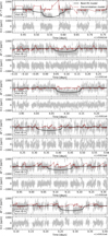 |
Fig. 1 CHEOPS light curves with spline decorrelation model (red) and best-fit transit model (black). The data from each CHEOPS visit (after removing outliers) is plotted in grey. Visit 1 has an overlapping transit of planets b and c; visits 2, 4, and 5 capture a transit of planet b; and visits 3 and 6 capture planet c. |
4.3 Transit and RV joint analysis
We performed a simultaneous fit of the previously detrended TESS photometry, the raw CHEOPS photometry, the raw HARPS and PFS RVs, the chosen stellar activity indicators, and the instrumental decorrelation parameters of CHEOPS (see Sect. 4.1) using the code LISA (Demangeon et al. 2018, 2021). The transits were modelled with the batman package (Kreidberg 2015) while the RV modelling used the radvel package (Fulton et al. 2018). We modelled the stellar activity using a Gaussian process (GP) as described in Sect. 4.3.2, which is fitted to the RV and the  data. In this analysis, we used a Bayesian inference framework that maximises the posterior probability. The parameter space was explored with the use of a Markov chain Monte Carlo (MCMC) algorithm implemented by the package emcee (Foreman-Mackey et al. 2013). We used a number of walkers that is four times greater than the number of parameters. To avoid a heavy computational load and too much memory usage while saving the chains and walkers, we performed a first initial run with 5000 steps, aimed at obtaining a rough estimation of the best-fit parameters. We then followed up with an additional 10 000 steps, starting from the median values from the initial run (excluding burn-in). The prior distributions are described in the following sections and a detailed summary of the values can be found in Table A.1.
4.3.1 Transit model
The transit model for each of the two planets was parameterised by the orbital period (P), the mid-transit time (T0), the cosine of the inclination (cos i), the planet-star radius ratio (Rp/R★), the products e sin ω and e cos ω, where e is the eccentricity and ω is the argument of the periastron, and the stellar density (ρ★). The limb-darkening was modelled with a quadratic law, with two coefficients for each instrument (u1 and u2). An additional jitter parameter and an offset parameter for the median flux were included in the model for each TESS sector and each CHEOPS visit.
We used a joint prior for the transit parameters (P, T0, cos i, ρ*), described as transiting prior in Demangeon et al. (2021). This joint prior effectively uses these parameters to compute the impact parameter (b) and the planetary orbital phase (ϕ) and allows us to define priors on b and ϕ instead of cos i and T0. We set ϕ = 0 to match the reference time, T0. We set a uniform prior for P and ϕ, ensuring the chains would not go out of the range of the CHEOPS observations during exploration and use a uniform prior for Rp/R★ between 0.01 and 0.03 (for planet b) or 0.04 (for planet c). A uniform distribution between 0 and 2 was chosen for b to allow for grazing transiting, with the additional condition that b < 1 + Rp/R★ to translate our prior knowledge that the planets are transiting. Similar to the transiting prior, a polar joint prior is used to convert e sin ω and e cos ω into e and ω. We set a beta distribution as the prior for e, with values of a = 0.867 and b = 3.03 using the formulation from Kipping (2013), and a uniform prior between −π and π for ω. For the limb-darkening coefficients, we set normal prior distributions whose mean and standard deviation were derived with the Limb-Darkening Toolkit (LDTk; Parviainen & Aigrain 2015), which estimates u1 and u2 from the effective temperature (Teff), gravity (log g), and metallicity ([Fe/H]) of the star, taking into account the response function of the instrument. We finally set a uniform prior for the jitter term, between zero and a value five times the median error from each data set, and a normal prior for each offset parameter.
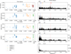 |
Fig. 2 Offset-corrected time series of the RV observations of HARPS and PFS (left), as well as the activity indicators of the HARPS RVs. For a preliminary analysis and plotting purposes, the offset between the different RV sets was estimated as the median of each time series. Corresponding GLS periodograms, computed from the offset-corrected values, as the offsets induce additional non-physical peaks that can potentially mask other relevant peaks (right). The window function is plotted in the last row. The vertical dashed lines show the approximate periods of the known planets as well as the expected stellar rotation period. The dashed horizontal lines show the 10% (dashed line), 1% (dot-dashed line), and 0.1% (dotted line) false-alarm probabilities as per Zechmeister & Kürster (2009). |
4.3.2 Radial velocity model
The model for the radial velocity analysis can be divided into three parts: the planetary model, the stellar activity model and the instrumental detrending. As we know, stellar activity is a major source of uncertainty when looking for planetary signals in RV measurements. We use an approach similar to the one in Demangeon et al. (2021), fitting a GP with a quasi-periodic kernel defined by:
![Mathematical equation: $K\left( {{t_i},{t_j}} \right) = {A^2}\exp \left[ { - {{{{\left( {{t_i} - {t_j}} \right)}^2}} \over {2\tau _{{\rm{decay }}}^2}} - {{{{\sin }^2}\left( {{\pi \over {{P_{{\rm{rdt }}}}}}\left| {{t_i} - {t_j}} \right|} \right)} \over {2{\gamma ^2}}}} \right],$](/articles/aa/full_html/2024/06/aa47759-23/aa47759-23-eq9.png) (1)
(1)
where A and Prot are the amplitude and the period of recurrence of the covariance, τdecay is the decay timescale, and γ is the periodic coherence scale. The amplitude, A, is related to the amplitude of the stellar activity signal and Prot to the stellar rotation period, making it a key parameter in the stellar activity model. We used two independent Gaussian processes with a quasi-periodic kernel implemented with the george package (Ambikasaran et al. 2015) to model the stellar variability: one for the  and the other for the RV data. While independent, the two GPs share some of their hyperparameters. The period of recurrence, the decay timescale, and the period coherence scale of the covariance are common to both GPs, while the amplitude of the covariance is different. The planetary signals were modelled with Keplerian orbit models and a systemic velocity (υ0). The Keplerian model is parameterised by the semi-amplitude of the RV signal (K), P, e sin ω, and e cos ω. For the instrumental model, we defined the first set of data (HARPS_0) as the reference, meaning υ0 is defined by this data set. We then defined an offset (ΔRV) between each data set and this reference set, which is particularly important to model the offset caused by the fibre change in HARPS as well as the fact that the PFS RVs are processed to be centred around zero. We fit the same offset value ΔRVHARPS_1 for the two HARPS data sets (67 measurements) after the fibre change. We chose to model the long-term trend in the RVs with a long-period sinusoidal function with the period, Psin, the semi-amplitude, Ksin, and the reference time, T0,sin, set as free parameters. The
  time series includes a second-degree polynomial trend with coefficients given by
  ,
,  , and
, and  . We also added a jitter parameter as we did for the transit model.
We set a Gaussian prior for each offset parameter, with the mean given by the difference between the average of each data set and a conservative standard deviation of 0.01 km s−1. As for the transit model, we put a uniform prior in the jitter parameter for each set of RVs, between zero and five times the average of the error of the data sets. The prior for υ0 was defined as a Gaussian distribution centred in the average value of the reference data set (HARPS_0), with a variance of 0.01 km s−1, as chosen for the offsets. For the hyperparameters of the kernel used for the Gaussian process model, we define a uniform prior between 0 and 0.01 km s−1 for the amplitude in the RV kernel and between 0 and 0.1 for the amplitude in the  kernel. The prior for the Prot parameter is set as uniform. The decay timescale was set to vary between 10 and 200 days with a uniform prior. For γ, the typical value is thought to be around 0.5 (Dubber et al. 2019), so we chose a uniform prior between 0.05 and 5, one order of magnitude below and above that value. We also set wide uniform priors for the free parameters of the sinusoidal trend in the RVs. Finally, we chose a uniform prior between 0 and 0.01 km s−1 for the amplitude of the planetary signals, as seen in Gandolfi et al. (2019). The remaining parameters of the planetary model are shared with the transit model and follow the priors described in Sect. 4.3.1.
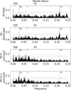 |
Fig. 3 GLS periodograms, computed from the offset-corrected values. The upper panel shows the raw periodogram of the RVs as shown in Fig. 2. The second panel shows the periodogram after the removal of the long-term trends (removed with a simple second-degree polynomial regression for pre-whitening purposes only). The lower panels show the periodograms after the removal of the Keplerian signals of HD 15337 b and c from the previous one. Vertical and horizontal lines as Fig. 2. |
4.3.3 Joint analysis results
The best-fit value of each of the parameters included in the joint analysis is obtained from the median of the posterior distribution, with the associated error corresponding to the 1σ confidence interval. A summary of the best-fit results can be found in Table 3 for the most relevant system and planet parameters, while the full results, including the posteriors of the detrending parameters and GP hyperparameters, are shown in Table A.1. Figure 4 shows the phase folded transits from TESS and CHEOPS with the best-fit transit model, while Figs. 5 and 6 show the full HARPS and PFS RV time series and the phase folded RVs for both planet models, respectively. Figure 7 shows the periodogram of the residuals of the RV fit, showing no peaks remaining near the planet periods or the stellar rotation period. All significant peaks shown in Figs. 2 and 3 that are not caused by orbiting planets were successfully removed by our GP model.
HD 15337 b has a measured radius of  and a mass of
  corresponding to a mean density of
  , consistent with a rocky planet with a thin atmosphere. For HD 15337 c, we obtain a radius of
  and a mass of
  , which gives a mean density of
  .
.
4.4 Internal structure model
Using the results from the joint analysis, we modelled the internal structure of HD 15337 b and c. We follow the method described in Leleu et al. (2021), which is based on Dorn et al. (2017). In the following, we briefly summarise the most important aspects of the model. Our internal structure model assumes each planet to be fully spherically symmetric and to consist of four fully distinct layers: an iron core modelled using equations of state from Hakim et al. (2018), a silicate mantle (Sotin et al. 2007), a water layer (Haldemann et al. 2020) and a pure H/He atmosphere as described in Lopez & Fortney (2014). We further assume that the Si/Mg/Fe ratios of each planet match the ones of the host star exactly (Thiabaud et al. 2015).
Our Bayesian inference model uses both stellar and planetary observables as input parameters, more specifically: the age, mass, radius, effective temperature, and abundances of the star and the transit depth, period, and mass relative to the star for each planet. We assumed a uniform prior for the mass fractions of the innermost three layers (iron core, mantle, and water), with the additional conditions that the sum of the three mass fractions is always one and the upper limit of the water mass fraction is 0.5 (Thiabaud et al. 2014; Marboeuf et al. 2014). For the mass of the H/He layer, we chose a prior that is uniform in log. Because of the intrinsic degeneracy of the problem, the results of the model do depend on the chosen priors and would differ if very different priors were chosen. The priors used in our analysis are provided in Table A.2. In Sect. 5, we discuss how different choices of priors and different model’s assumptions would affect our results. Furthermore, we model both planets simultaneously.
The resulting posterior distributions from our internal structure analysis for HD 15337 b and c are shown in Figs. 8 and 9, where the errors correspond to the 5th and 95th percentiles. We found a core mass fraction (fmcore) of  for planet b and
  for planet c. While our models show that the mass of H/He (mgas) in HD 15337 b is negligibly small, the planet may host a water layer, as the mass fraction with respect to the solid part of the planet (fmwater) is
  . Conversely, for HD 15337 c the water mass fraction is almost completely unconstrained at
  , while the planet seems to host a significant H/He layer with a mass of
  and a thickness of
  . The posteriors of the internal structure best-fit model are summarised in Table A.2.
HD 15337 system parameters from the joint fit of transits and RVs.
5 Discussion
The high-precision photometry measurements from CHEOPS allow us to improve the radius precision of HD 15337 b from the ~3.5% from Gandolfi et al. (2019) and Dumusque et al. (2019) to 1.8%, turning it into one of the highest precision radius measurements for super-Earths. HD 15337 c also improved its radius precision to 3%. With this, both planets are now under the 3% threshold for radius precision, which is key to improving the constraint on the water mass fraction (Dorn et al. 2017). We also significantly improved the mass precision of HD 15337 b with the help of the new HARPS and PFS data. Measured at around 11–13% by Gandolfi et al. (2019) and Dumusque et al. (2019), the mass uncertainty from our analysis is around half those values, sitting at 6.5%. While there was an improvement in the mass uncertainty of HD 15337 c, we were only able to reach a precision of 17%, very similar to the 19–21% obtained by the mentioned authors. We note that the median value of our masses is lower on both planets than what was measured before. Gandolfi et al. (2019) reported a mass of  for HD 15337 b, with Dumusque et al. (2019) providing a similar value and uncertainty at Mb = 7.20 ± 0.81 M⊕. For HD 15337 c, the difference is larger but still within the 1σ range of the result of Dumusque et al. (2019), Mc = 8.79 ± 1.68 M⊕. As expected, the new RV measurements from HARPS and PFS allow for a stronger constraint to be placed on the long-term trends, as well as the stellar activity signals by expanding the temporal range; the latter, in turn, allows for a better fit of the RV signal of both planets, leading to a more accurate result. We can also see that while the masses of both planets are similar, HD 15337 c has a radius that is ∽1.4 times larger than HD 15337 b. This results in a lower density, suggesting a planet with a more significant water layer and gas envelope.
The long-term trend shown in the RV time series is most likely caused by stellar activity, as mentioned before, given the same type of trend is also present in the FWHM indicator. Alternatively, it is possible that the signal is being caused by a long-period companion. A stellar companion could explain the trend seen in FWHM if the radial velocity of the companion is close enough to the target star. However, for a planetary companion, the FWHM trend would have to be due to the instrument and the correlation with the RV trend would have to be coincidental.
As stated in Sect. 4.3.2, the trend was modelled with a sinusoidal function, whose best-fit results show a period of  yr and a semi-amplitude of
  km s−1, an order of magnitude higher than the RV signature of the two planets. If we assume this trend is caused by a long-period companion, we estimate its minimum mass to be M sin i = 4 MJup. It would be theoretically possible that this trend was caused by the stellar companion described in Sect. 3, but we find that with a period of 540 yr (Lester et al. 2021), the orbit would need to be eccentric to produce such a trend in the time span of the HARPS observations (∽16 yr). We estimated the amplitude of the signal caused by the stellar companion, given the mass ratio of 0.14 from Lester et al. (2021). This is one order of magnitude higher than the amplitude we found in the current RVs, which could be the case for an eccentric orbit. Therefore, it is unclear that this companion is the cause of the RV trend. Initially, this trend was modelled as a second-degree polynomial as in Gandolfi et al. (2019), which provides consistent results (at 1σ) with the sinusoidal model. We decided to adopt the sinusoidal model as it provides a more direct constraint on the hypothesis of a gravitationally bound companion.
The periodogram of the RV residuals (Fig. 7) shows some hints at the periods of 6.73, 6.15, and 5.53 days. These peaks were not detected before the removal of the planetary and stellar activity signals and are also not present in the periodograms of the indicators. However, since they are below the 0.1% FAP level, there is not enough evidence of a statistically significant signal at these periods (Baluev 2008). They also do not correspond to aliases of the stellar rotation period and it is unlikely that they are of a planetary nature, given the proximity to the orbit of HD 15337 b and no hint of a transit around those periods in the TESS light curves. As such, the nature of these peaks is currently unknown.
Figure 10 shows the position of HD 15337 b and HD 15337 c in the mass-radius diagram compared to other small planets with a mass precision of <25%7. The composition models from Zeng et al. (2016) are overplotted ranging from a full iron composition to a full water world, to provide a general view of the position of each planet in the field. HD 15337 b is located on the upper range of the super-Earth population below the radius gap (Fulton et al. 2017), lying close to the pure silicate line from the model of Zeng et al. (2016). HD 15337 c on the other hand is placed within the sub-Neptune population, on the other side of the radius gap and above the predicted 100% water line, hinting at the presence of a gas envelope. The results of our internal structure analysis agree with the position of both planets in the MR diagram, as we find a H/He layer in planet c with a significant water layer and we confirm planet b to be in the super-Earth population. Despite lying near the pure silicate line, according to the models from Zeng et al. (2016), HD 15337 b shows a relatively high iron mass fraction in both core and mantle with our model.
Our internal structure model includes liquid phases in the EOS of the inner core and the water layer, but we fixed the temperature and pressure to 300 K and 1 bar outside the water layer and modelled the gas layer separately from the rest of the planet. As HD 15337 b orbits close to its star, the high irradiation causes it to reach high equilibrium temperatures (~1000 K). At these temperatures, it is highly unlikely that the water is fully condensed, and with a density that is below Earth’s density, this planet may have a molten mantle with water present in it. To tackle this problem, Dorn & Lichtenberg (2021) presented an internal structure model that takes into account this aspect and shows that the presence of water in the mantle can lead to a significant underestimation of the water mass fraction given the same observed mass and radius. Determining the water content of exoplanets with a reasonable level of accuracy is particularly relevant in the search for habitable worlds and can affect dynamic and structural properties, such as the differentiation between core and mantle (Bonati et al. 2021) and atmospheric composition (Gaillard et al. 2021). For a planet with the mass and radius of HD 15337 b, Dorn & Lichtenberg (2021) predicted a water mass fraction 15–20% higher than that obtained with our model. It should be noted that this difference appears to be smaller for more massive planets.
Another assumption we made in our model is that the abundances of the planets are exactly the same as the host star. However, Adibekyan et al. (2021) showed that while there is a correlation, it is unlikely to be a 1:1 relationship, and the ratios of Si/Mg/Fe may not necessarily match the ones from the star. We performed a new run of the internal structure model for both planets without constraining the abundances to compare the results. We saw that without the priors in the abundances, both planets share a similar range of values in the posterior of the core mass fraction. However, the distribution indicates that smaller mass fractions are accepted more often than before. The same is true for the water mass fraction of HD 15337 b, with the posterior being indistinguishable from zero at a 2σ confidence level. It is therefore more likely that there is not a significant water layer on this planet, compared to what the model with constrained abundances has shown. We also note an increase in the range in the mantle mass fraction, compensating for the smaller core and water fractions. The mass of the gas envelope of HD 15337 c does not show significant changes.
It has been suggested that HD 15337 b could host a secondary atmosphere, after losing its initial H/He envelope to photo evaporation (Dumusque et al. 2019). Confirming this would require further research into the evolution of these planets and the real composition of the gas envelope present in HD 15337 c.
We provide improved limits on radius, mass and internal structure and composition parameters that should provide a strong basis for follow-up studies. HD 15337 is expected to be observed once again, this time by JWST, which could further improve these limits and potentially provide enough data to better constrain the evolution and formation of this system.
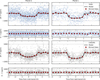 |
Fig. 4 Phase-folded light curves from TESS (upper panels) and CHEOPS (lower panels) measurements. The best-fit model of the transit is plotted in black for HD 15337 b (left) and HD 15337 c (right). The bottom panels for each instrument show the residuals of the best-fit model. We over-plot the binned light curves and residuals with 20-min bins. |
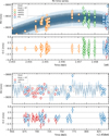 |
Fig. 5 Full RV time series for HD 15337 corrected for instrumental variability. The best-fit model with both Keplerian signals and the model with the stellar activity GP are over-plotted in blue and light blue respectively. Bottom panels: zoom on the most recent HARPS and PFS data. |
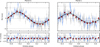 |
Fig. 6 Phase-folded radial velocity curves (top) from HARPS (grey dots) and PFS (blue dots) measurements. The best-fit model of the Keplerian signal is plotted in black for HD 15337 b (left) and HD 15337 c (right). The bottom panel shows the residuals of the best-fit model as in Fig. 4. We over-plot the binned data and residuals. |
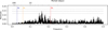 |
Fig. 7 Periodogram of the residuals from the RV fit. There are no longer any peaks at the orbital periods of the planet or the stellar rotation period, showing a good fit from the GP and the Keplerian models. Horizontal lines show the FAP thresholds as in Fig. 2. |
6 Summary
In this paper, we use all available measurements of HD 15337 obtained from CHEOPS, HARPS, and PFS to perform a joint fit of the transits and RVs of the HD 15337 system. We significantly improve the precision of the radius and mass of HD 15337 b, to 1.7% and 6.2%, respectively. We also improve the precision of the radius of HD 15337 c to 3%, but we were unable to decrease the mass uncertainties despite the additional RV points, sitting at ~18%. With our internal structure model fitting both planets at the same time, we find that HD 15337 b is most likely a rocky planet. In addition, while our calculations show a water mass fraction higher than zero at a 2σ level, the planet is also compatible with a dry composition. We also find that while the water mass fraction of HD 15337 c remains unconstrained, the model reveals a gaseous envelope with a mass higher than 0.01 M⊕. We conclude that the results of the internal structure analysis are highly dependent on the model and the applied assumptions.
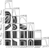 |
Fig. 8 Posterior distribution of the most important internal structure parameters for HD 15337 b. The parameters depicted are the mass fractions of the inner iron core and water layer with respect to the solid part of the planet (which together with the mass fraction of the silicate mantle add up to 1), the molar fractions of Si and Mg in the mantle layer and Fe in the inner iron core and the logarithm with base 10 of the total mass of the H/He layer in Earth masses. The values and errors on top of each column correspond to the median and the 5th and 95th percentiles. |
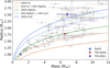 |
Fig. 10 Mass-radius plot showing the position of HD 15337 b and HD 15337 c compared to other small exoplanets. |
Acknowledgements
CHEOPS is an ESA mission in partnership with Switzerland with important contributions to the payload and the ground segment from Austria, Belgium, France, Germany, Hungary, Italy, Portugal, Spain, Sweden, and the United Kingdom. The CHEOPS Consortium would like to gratefully acknowledge the support received by all the agencies, offices, universities, and industries involved. Their flexibility and willingness to explore new approaches were essential to the success of this mission. This work was supported by FCT – Fundação para a Ciência e a Tecnologia through national funds by these grants: UIDB/04434/2020, UIDP/04434/2020, 2022.06962. PTDC, 2022.04416.PTDC. N.M.R. acknowledges support from FCT through grant DFA/BD/5472/2020. O.D.S.D. is supported in the form of work contract (DL 57/2016/CP1364/CT0004) funded by national funds through FCT. S.C.C.B. acknowledges support from FCT through FCT contracts nr. IF/01312/2014/CP1215/CT0004. D.G. gratefully acknowledges financial support from the CRT foundation under Grant No. 2018.2323 “Gaseous or rocky? Unveiling the nature of small worlds”. J.A.Eg. and Y.Al. acknowledge support from the Swiss National Science Foundation (SNSF) under grant 200020_192038. LMS gratefully acknowledges financial support from the CRT foundation under Grant No. 2018.2323 “Gaseous or rocky? Unveiling the nature of small worlds”. This work has been carried out within the framework of the NCCR PlanetS supported by the Swiss National Science Foundation under grants 51NF40_182901 and 51NF40_205606. T.Wi. and A.C.Ca. acknowledge support from STFC consolidated grant numbers ST/R000824/1 and ST/V000861/1, and UKSA grant number ST/R003203/1. The Belgian participation to CHEOPS has been supported by the Belgian Federal Science Policy Office (BELSPO) in the framework of the PRODEX Program, and by the University of Liège through an ARC grant for Concerted Research Actions financed by the Wallonia-Brussels Federation. L.D. is an F.R.S.-FNRS Postdoctoral Researcher. NCSa acknowledges funding by the European Union (ERC, FIERCE, 101052347). Views and opinions expressed are however those of the author(s) only and do not necessarily reflect those of the European Union or the European Research Council. Neither the European Union nor the granting authority can be held responsible for them. S.G.S. acknowledges support from FCT through FCT contract nr. CEECIND/00826/2018 and POPH/FSE (EC). V.A. is supported by FCT through national funds by the following grant: 2022.06962.PTDC (http://doi.org/10.54499/2022.06962.PTDC). RAl, DBa, EPa, and IRi acknowledge financial support from the Agencia Estatal de Investigación of the Ministerio de Ciencia e Innovación MCIN/AEI/10.13039/501100011033 and the ERDF “A way of making Europe” through projects PID2019-107061GB-C61, PID2019-107061GB-C66, PID2021-125627OB-C31, and PID2021-125627OB-C32, from the Centre of Excellence “Severo Ochoa” award to the Instituto de Astrofísica de Canarias (CEX2019-000920-S), from the Centre of Excellence “María de Maeztu” award to the Institut de Ciències de l’Espai (CEX2020-001058-M), and from the Generalitat de Catalunya/CERCA programme. X.B., S.C., D.G., M.F. and J.L. acknowledge their role as ESA-appointed CHEOPS science team members. L.Bo., V.Na., I.Pa., G.Pi., R.Ra., and G.Sc. acknowledge support from CHEOPS ASI-INAF agreement no. 2019-29-HH.0. P.E.C. is funded by the Austrian Science Fund (FWF) Erwin Schroedinger Fellowship, program J4595-N. ABr was supported by the SNSA. This project was supported by the CNES. B.-O.D. acknowledges support from the Swiss State Secretariat for Education, Research and Innovation (SERI) under contract number MB22.00046. This project has received funding from the European Research Council (ERC) under the European Union’s Horizon 2020 research and innovation programme (project FOUR ACES, grant agreement no. 724427). It has also been carried out in the frame of the National Centre for Competence in Research PlanetS supported by the Swiss National Science Foundation (SNSF). DE acknowledges financial support from the Swiss National Science Foundation for project 200021_200726. MF and CMP gratefully acknowledge the support of the Swedish National Space Agency (DNR 65/19, 174/18). M.G. is an F.R.S.-FNRS Senior Research Associate. MNG is the ESA CHEOPS Project Scientist and Mission Representative, and as such also responsible for the Guest Observers (GO) Programme. MNG does not relay proprietary information between the GO and Guaranteed Time Observation (GTO) Programmes, and does not decide on the definition and target selection of the GTO Programme. CHe acknowledges support from the European Union H2020-MSCA-ITN-2019 under Grant Agreement no. 860470 (CHAMELEON). SH gratefully acknowledges CNES funding through the grant 837319. KGI is the ESA CHEOPS Project Scientist and is responsible for the ESA CHEOPS Guest Observers Programme. She does not participate in, or contribute to, the definition of the Guaranteed Time Programme of the CHEOPS mission through which observations described in this paper have been taken, nor to any aspect of target selection for the programme. K.W.F.L. was supported by Deutsche Forschungsgemeinschaft grants RA714/14-1 within the DFG Schwerpunkt SPP 1992, Exploring the Diversity of Extrasolar Planets. This work was granted access to the HPC resources of MesoPSL financed by the Region Ile de France and the project Equip@Meso (reference ANR-10-EQPX-29-01) of the programme Investissements d'Avenir supervised by the Agence Nationale pour la Recherche. M.L. acknowledges support of the Swiss National Science Foundation under grant number PCEFP2_194576. P.M. acknowledges support from STFC research grant number ST/M001040/1. This work was also partially supported by a grant from the Simons Foundation (PI Queloz, grant number 327127). GyMSz acknowledges the support of the Hungarian National Research, Development and Innovation Office (NKFIH) grant K-125015, a PRODEX Experiment Agreement No. 4000137122, the Lendület LP2018-7/2021 grant of the Hungarian Academy of Science and the support of the city of Szombathely. V.V.G. is an F.R.S-FNRS Research Associate. NAW acknowledges UKSA grant ST/R004838/1. AN and JV acknowledge support from the Swiss National Science Foundation (SNSF) under grant PZ00P2_208945.
Appendix A Additional Tables
Priors used for the joint transit and RV modelling and corresponding posteriors from the best-fit model.
Priors used for the internal structure modelling and corresponding posteriors from the best-fit model with error bars corresponding to the 5% and 95% percentiles.
References
- Adibekyan, V. Z., Sousa, S. G., Santos, N. C., et al. 2012, A&A, 545, A32 [NASA ADS] [CrossRef] [EDP Sciences] [Google Scholar]
- Adibekyan, V., Figueira, P., Santos, N. C., et al. 2015, A&A, 583, A94 [NASA ADS] [CrossRef] [EDP Sciences] [Google Scholar]
- Adibekyan, V., Dorn, C., Sousa, S. G., et al. 2021, Science, 374, 330 [NASA ADS] [CrossRef] [Google Scholar]
- Allard, F. 2014, in Exploring the Formation and Evolution of Planertary Systems, 299, eds. M. Booth, B. C. Matthews, & J. R. Graham, 271 [NASA ADS] [Google Scholar]
- Ambikasaran, S., Foreman-Mackey, D., Greengard, L., Hogg, D. W., & O’Neil, M. 2015, IEEE Trans. Pattern Anal. Mach. Intell., 38, 252 [Google Scholar]
- Angus, R., Morton, T. D., Foreman-Mackey, D., et al. 2019, AJ, 158, 173 [Google Scholar]
- Baluev, R. V. 2008, MNRAS, 385, 1279 [Google Scholar]
- Baranne, A., Queloz, D., Mayor, M., et al. 1996, A&AS, 119, 373 [NASA ADS] [CrossRef] [EDP Sciences] [Google Scholar]
- Barnes, S. A. 2010, ApJ, 722, 222 [Google Scholar]
- Barros, S., Demangeon, O., Alibert, Y., et al. 2022, A&A, 665, A154 [NASA ADS] [CrossRef] [EDP Sciences] [Google Scholar]
- Benz, W., Broeg, C., Fortier, A., et al. 2021, Exp. Astron., 51, 109 [Google Scholar]
- Blackwell, D. E., & Shallis, M. J. 1977, MNRAS, 180, 177 [NASA ADS] [CrossRef] [Google Scholar]
- Bonati, I., Lasbleis, M., & Noack, L. 2021, J. Geophys. Res.: Planets, 126, e2020JE006724 [Google Scholar]
- Bonfanti, A., Ortolani, S., Piotto, G., & Nascimbeni, V. 2015, A&A, 575, A18 [NASA ADS] [CrossRef] [EDP Sciences] [Google Scholar]
- Bonfanti, A., Ortolani, S., & Nascimbeni, V. 2016, A&A, 585, A5 [NASA ADS] [CrossRef] [EDP Sciences] [Google Scholar]
- Bonfanti, A., Delrez, L., Hooton, M. J., et al. 2021, A&A, 646, A157 [EDP Sciences] [Google Scholar]
- Borucki, W. J. 2016, Rep. Progr. Phys., 79, 036901 [Google Scholar]
- Butler, R. P., Marcy, G. W., Williams, E., et al. 1996, PASP, 108, 500 [Google Scholar]
- Castelli, F., & Kurucz, R. L. 2003, in IAU Symp., 210, Modelling of Stellar Atmospheres, eds. N. Piskunov, W. W. Weiss, & D. F. Gray, A20 [Google Scholar]
- Ciardi, D. R., Beichman, C. A., Horch, E. P., & Howell, S. B. 2015, ApJ, 805, 16 [NASA ADS] [CrossRef] [Google Scholar]
- Crane, J. D., Shectman, S. A., & Butler, R. P. 2006, in Ground-based and Airborne Instrumentation for Astronomy, 6269, SPIE, 972 [Google Scholar]
- Crane, J. D., Shectman, S. A., Butler, R. P., Thompson, I. B., & Burley, G. S. 2008, in Ground-based and Airborne Instrumentation for Astronomy II, 7014, SPIE, 2484 [Google Scholar]
- Crane, J. D., Shectman, S. A., Butler, R. P., et al. 2010, in Ground-based and Airborne Instrumentation for Astronomy III, 7735, SPIE, 1909 [Google Scholar]
- Demangeon, O. D., Faedi, F., Hébrard, G., et al. 2018, A&A, 610, A63 [NASA ADS] [CrossRef] [EDP Sciences] [Google Scholar]
- Demangeon, O. D., Osorio, M. Z., Alibert, Y., et al. 2021, A&A, 653, A41 [NASA ADS] [CrossRef] [EDP Sciences] [Google Scholar]
- Dorn, C., & Lichtenberg, T. 2021, ApJ, 922, L4 [NASA ADS] [CrossRef] [Google Scholar]
- Dorn, C., Venturini, J., Khan, A., et al. 2017, A&A, 597, A37 [NASA ADS] [CrossRef] [EDP Sciences] [Google Scholar]
- Dubber, S. C., Mortier, A., Rice, K., et al. 2019, MNRAS, 490, 5103 [NASA ADS] [CrossRef] [Google Scholar]
- Dumusque, X., Turner, O., Dorn, C., et al. 2019, A&A, 627, A43 [NASA ADS] [CrossRef] [EDP Sciences] [Google Scholar]
- Foreman-Mackey, D., Hogg, D. W., Lang, D., & Goodman, J. 2013, PASP, 125, 306 [Google Scholar]
- Fulton, B. J., Petigura, E. A., Howard, A. W., et al. 2017, AJ, 154, 109 [Google Scholar]
- Fulton, B. J., Petigura, E. A., Blunt, S., & Sinukoff, E. 2018, PASP, 130, 044504 [Google Scholar]
- Gaia Collaboration (Brown, A. G. A., et al.) 2016, A&A, 595, A2 [NASA ADS] [CrossRef] [EDP Sciences] [Google Scholar]
- Gaia Collaboration 2020, VizieR Online Data Catalog: I/350 [Google Scholar]
- Gaia Collaboration (Brown, A. G. A., et al.) 2021, A&A, 649, A1 [NASA ADS] [CrossRef] [EDP Sciences] [Google Scholar]
- Gaia Collaboration (Vallenari, A., et al.) 2023, A&A, 674, A1 [NASA ADS] [CrossRef] [EDP Sciences] [Google Scholar]
- Gaillard, F., Bouhifd, M. A., Füri, E., et al. 2021, Space Sci. Rev., 217, 1 [NASA ADS] [CrossRef] [Google Scholar]
- Gandolfi, D., Barragán, O., Hatzes, A. P., et al. 2017, AJ, 154, 123 [NASA ADS] [CrossRef] [Google Scholar]
- Gandolfi, D., Fossati, L., Livingston, J. H., et al. 2019, ApJ, 876, L24 [Google Scholar]
- Hakim, K., Rivoldini, A., Van Hoolst, T., et al. 2018, Icarus, 313, 61 [Google Scholar]
- Haldemann, J., Alibert, Y., Mordasini, C., & Benz, W. 2020, A&A, 643, A105 [NASA ADS] [CrossRef] [EDP Sciences] [Google Scholar]
- Hoyer, S., Guterman, P., Demangeon, O., et al. 2020, A&A, 635, A24 [NASA ADS] [CrossRef] [EDP Sciences] [Google Scholar]
- Jenkins, J. M. 2020, Kepler Science Document KSCI-19081-003, 2 [Google Scholar]
- Kipping, D. M. 2013, MNRAS, 434, L51 [Google Scholar]
- Kreidberg, L. 2015, PASP, 127, 1161 [Google Scholar]
- Kuerster, M., Endl, M., Rouesnel, F., et al. 2003, A&A, 403, 1077 [NASA ADS] [CrossRef] [EDP Sciences] [Google Scholar]
- Kurucz, R. L. 1993, SYNTHE spectrum synthesis programs and line data (Cambridge, Mass.: Smithsonian Astrophysical Observatory) [Google Scholar]
- Lee, E. J., & Chiang, E. 2016, ApJ, 817, 90 [Google Scholar]
- Leleu, A., Alibert, Y., Hara, N. C., et al. 2021, A&A, 649, A26 [NASA ADS] [CrossRef] [EDP Sciences] [Google Scholar]
- Lester, K. V., Matson, R. A., Howell, S. B., et al. 2021, AJ, 162, 75 [NASA ADS] [CrossRef] [Google Scholar]
- Lindegren, L., Bastian, U., Biermann, M., et al. 2021, A&A, 649, A4 [EDP Sciences] [Google Scholar]
- Liu, S.-F., Hori, Y., Lin, D., & Asphaug, E. 2015, ApJ, 812, 164 [CrossRef] [Google Scholar]
- Lo Curto, G., Pepe, F., Avila, G., et al. 2015, The Messenger, 162, 9 [NASA ADS] [Google Scholar]
- Lopez, E. D., & Fortney, J. J. 2014, ApJ, 792, 1 [Google Scholar]
- Lovis, C., & Pepe, F. 2007, A&A, 468, 1115 [NASA ADS] [CrossRef] [EDP Sciences] [Google Scholar]
- Luque, R., & Pallé, E. 2022, Science, 377, 1211 [NASA ADS] [CrossRef] [Google Scholar]
- Marboeuf, U., Thiabaud, A., Alibert, Y., Cabral, N., & Benz, W. 2014, A&A, 570, A36 [NASA ADS] [CrossRef] [EDP Sciences] [Google Scholar]
- Marigo, P., Girardi, L., Bressan, A., et al. 2017, ApJ, 835, 77 [Google Scholar]
- Mayor, M., Pepe, F., Queloz, D., et al. 2003, The Messenger, 114, 20 [NASA ADS] [Google Scholar]
- McQuillan, A., Mazeh, T., & Aigrain, S. 2014, ApJS, 211, 24 [Google Scholar]
- Morris, B., Delrez, L., Brandeker, A., et al. 2021, A&A, 653, A173 [NASA ADS] [CrossRef] [EDP Sciences] [Google Scholar]
- Owen, J. E., & Wu, Y. 2017, ApJ, 847, 29 [Google Scholar]
- Parviainen, H., & Aigrain, S. 2015, MNRAS, 453, 3821 [Google Scholar]
- Pepe, F., Mayor, M., Galland, F., et al. 2002, A&A, 388, 632 [NASA ADS] [CrossRef] [EDP Sciences] [Google Scholar]
- Ricker, G. R., Winn, J. N., Vanderspek, R., et al. 2014, J. Astron. Telescopes Instrum. Syst., 1, 014003 [NASA ADS] [CrossRef] [Google Scholar]
- Rosário, N. M., Barros, S. C. C., Demangeon, O. D. S., & Santos, N. C. 2022, A&A, 668, A114 [NASA ADS] [CrossRef] [EDP Sciences] [Google Scholar]
- Salmon, S. J. A. J., Van Grootel, V., Buldgen, G., Dupret, M. A., & Eggenberger, P. 2021, A&A, 646, A7 [NASA ADS] [CrossRef] [EDP Sciences] [Google Scholar]
- Santos, N. C., Sousa, S. G., Mortier, A., et al. 2013, A&A, 556, A150 [NASA ADS] [CrossRef] [EDP Sciences] [Google Scholar]
- Santos, A., Breton, S., Mathur, S., & García, R. 2021, ApJS, 255, 17 [NASA ADS] [CrossRef] [Google Scholar]
- Schanche, N., Hébrard, G., Collier Cameron, A., et al. 2020, MNRAS, 499, 428 [NASA ADS] [CrossRef] [Google Scholar]
- Scuflaire, R., Théado, S., Montalbán, J., et al. 2008, Ap&SS, 316, 83 [Google Scholar]
- Skrutskie, M. F., Cutri, R. M., Stiening, R., et al. 2006, AJ, 131, 1163 [NASA ADS] [CrossRef] [Google Scholar]
- Smith, J. C., Stumpe, M. C., Van Cleve, J. E., et al. 2012, PASP, 124, 1000 [Google Scholar]
- Smith, J. C., Morris, R. L., Jenkins, J. M., et al. 2017, Kepler Science Document KSCI-19081-002, 7 [Google Scholar]
- Sneden, C. A. 1973, PhD thesis, The University of Texas at Austin, USA [Google Scholar]
- Sotin, C., Grasset, O., & Mocquet, A. 2007, Icarus, 191, 337 [Google Scholar]
- Soubiran, C., Jasniewicz, G., Chemin, L., et al. 2018, A&A, 616, A7 [NASA ADS] [CrossRef] [EDP Sciences] [Google Scholar]
- Sousa, S. G., Santos, N. C., Israelian, G., Mayor, M., & Monteiro, M. J. P. F. G. 2007, A&A, 469, 783 [NASA ADS] [CrossRef] [EDP Sciences] [Google Scholar]
- Sousa, S. G., Santos, N. C., Adibekyan, V., Delgado-Mena, E., & Israelian, G. 2015, A&A, 577, A67 [NASA ADS] [CrossRef] [EDP Sciences] [Google Scholar]
- Sousa, S., Adibekyan, V., Delgado-Mena, E., et al. 2018, A&A, 620, A58 [NASA ADS] [CrossRef] [EDP Sciences] [Google Scholar]
- Sousa, S. G., Adibekyan, V., Delgado-Mena, E., et al. 2021, A&A, 656, A53 [NASA ADS] [CrossRef] [EDP Sciences] [Google Scholar]
- Tenenbaum, P., & Jenkins, J. M. 2018, TESS Science Data Products Description Document, EXP-TESS-ARC-ICD-0014 RevD, NASA/TM-2018-220036 [Google Scholar]
- Teske, J., Wang, S. X., Wolfgang, A., et al. 2021, ApJS, 256, 33 [NASA ADS] [CrossRef] [Google Scholar]
- Thiabaud, A., Marboeuf, U., Alibert, Y., et al. 2014, A&A, 562, A27 [NASA ADS] [CrossRef] [EDP Sciences] [Google Scholar]
- Thiabaud, A., Marboeuf, U., Alibert, Y., Leya, I., & Mezger, K. 2015, A&A, 574, A138 [NASA ADS] [CrossRef] [EDP Sciences] [Google Scholar]
- Tsantaki, M., Sousa, S. G., Adibekyan, V. Z., et al. 2013, A&A, 555, A150 [NASA ADS] [CrossRef] [EDP Sciences] [Google Scholar]
- Venturini, J., Guilera, O. M., Haldemann, J., Ronco, M. P., & Mordasini, C. 2020. A&A, 643, A1 [Google Scholar]
- Wright, E. L., Eisenhardt, P. R. M., Mainzer, A. K., et al. 2010, AJ, 140, 1868 [Google Scholar]
- Zechmeister, M., & Kürster, M. 2009, A&A, 496, 577 [CrossRef] [EDP Sciences] [Google Scholar]
- Zeng, L., Sasselov, D. D., & Jacobsen, S. B. 2016, ApJ, 819, 127 [Google Scholar]
- Ziegler, C., Tokovinin, A., Briceño, C., et al. 2020, AJ, 159, 19 [Google Scholar]
DRP version 13.
We adopted a B–V colour index of 0.880.
Automatic Routine for Line Equivalent Widths in Stellar Spectra. The latest version, ARES v2, can be downloaded at https://github.com/sousasag/ARES
PAdova and TRieste Stellar Evolutionary Code: http://stev.oapd.inaf.it/cgi-bin/cmd
Value inferred using the definition of the transit depth for a binary system (i.e., with the two stellar fluxes in the denominator), and imposing the radius of the planet equal to the radius of the secondary, as an extreme limiting case.
All Tables
Priors used for the joint transit and RV modelling and corresponding posteriors from the best-fit model.
Priors used for the internal structure modelling and corresponding posteriors from the best-fit model with error bars corresponding to the 5% and 95% percentiles.
All Figures
|
Fig. 1 CHEOPS light curves with spline decorrelation model (red) and best-fit transit model (black). The data from each CHEOPS visit (after removing outliers) is plotted in grey. Visit 1 has an overlapping transit of planets b and c; visits 2, 4, and 5 capture a transit of planet b; and visits 3 and 6 capture planet c. |
| In the text | |
|
Fig. 2 Offset-corrected time series of the RV observations of HARPS and PFS (left), as well as the activity indicators of the HARPS RVs. For a preliminary analysis and plotting purposes, the offset between the different RV sets was estimated as the median of each time series. Corresponding GLS periodograms, computed from the offset-corrected values, as the offsets induce additional non-physical peaks that can potentially mask other relevant peaks (right). The window function is plotted in the last row. The vertical dashed lines show the approximate periods of the known planets as well as the expected stellar rotation period. The dashed horizontal lines show the 10% (dashed line), 1% (dot-dashed line), and 0.1% (dotted line) false-alarm probabilities as per Zechmeister & Kürster (2009). |
| In the text | |
|
Fig. 3 GLS periodograms, computed from the offset-corrected values. The upper panel shows the raw periodogram of the RVs as shown in Fig. 2. The second panel shows the periodogram after the removal of the long-term trends (removed with a simple second-degree polynomial regression for pre-whitening purposes only). The lower panels show the periodograms after the removal of the Keplerian signals of HD 15337 b and c from the previous one. Vertical and horizontal lines as Fig. 2. |
| In the text | |
|
Fig. 4 Phase-folded light curves from TESS (upper panels) and CHEOPS (lower panels) measurements. The best-fit model of the transit is plotted in black for HD 15337 b (left) and HD 15337 c (right). The bottom panels for each instrument show the residuals of the best-fit model. We over-plot the binned light curves and residuals with 20-min bins. |
| In the text | |
|
Fig. 5 Full RV time series for HD 15337 corrected for instrumental variability. The best-fit model with both Keplerian signals and the model with the stellar activity GP are over-plotted in blue and light blue respectively. Bottom panels: zoom on the most recent HARPS and PFS data. |
| In the text | |
|
Fig. 6 Phase-folded radial velocity curves (top) from HARPS (grey dots) and PFS (blue dots) measurements. The best-fit model of the Keplerian signal is plotted in black for HD 15337 b (left) and HD 15337 c (right). The bottom panel shows the residuals of the best-fit model as in Fig. 4. We over-plot the binned data and residuals. |
| In the text | |
|
Fig. 7 Periodogram of the residuals from the RV fit. There are no longer any peaks at the orbital periods of the planet or the stellar rotation period, showing a good fit from the GP and the Keplerian models. Horizontal lines show the FAP thresholds as in Fig. 2. |
| In the text | |
|
Fig. 8 Posterior distribution of the most important internal structure parameters for HD 15337 b. The parameters depicted are the mass fractions of the inner iron core and water layer with respect to the solid part of the planet (which together with the mass fraction of the silicate mantle add up to 1), the molar fractions of Si and Mg in the mantle layer and Fe in the inner iron core and the logarithm with base 10 of the total mass of the H/He layer in Earth masses. The values and errors on top of each column correspond to the median and the 5th and 95th percentiles. |
| In the text | |
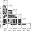 |
Fig. 9 Same as Fig. 8 but for HD 15337 c. |
| In the text | |
|
Fig. 10 Mass-radius plot showing the position of HD 15337 b and HD 15337 c compared to other small exoplanets. |
| In the text | |
Current usage metrics show cumulative count of Article Views (full-text article views including HTML views, PDF and ePub downloads, according to the available data) and Abstracts Views on Vision4Press platform.
Data correspond to usage on the plateform after 2015. The current usage metrics is available 48-96 hours after online publication and is updated daily on week days.
Initial download of the metrics may take a while.