| Issue |
A&A
Volume 686, June 2024
|
|
|---|---|---|
| Article Number | A292 | |
| Number of page(s) | 26 | |
| Section | Extragalactic astronomy | |
| DOI | https://doi.org/10.1051/0004-6361/202347034 | |
| Published online | 20 June 2024 | |
What can be learnt from UHECR anisotropies observations
II. Intermediate-scale anisotropies
Université Paris Cité, CNRS, Laboratoire Astroparticule et Cosmologie, 75013 Paris, France
e-mail: allard@apc.in2p3.fr
Received:
28
May
2023
Accepted:
2
April
2024
Context. Various signals of anisotropy of the ultra-high-energy cosmic rays (UHECRs) have recently been reported, whether at large angular scales, with a dipole modulation in right ascension observed in the data of the Pierre Auger observatory (Auger), as discussed in the first paper accompanying the present one, or at intermediate angular scales, with flux excesses identified in specific directions by Auger and the Telescope Array (TA) Collaborations.
Aims. We investigated the implications of the current data regarding these intermediate scale anisotropies, and examined to what extent they can be used to shed light on the origin of UHECRs, and constrain the astrophysical and/or physical parameters of the viable source scenarios. We also investigated what could be learnt from the study of the evolution of the various UHECR anisotropy signals, and discussed the expected benefit of an increased exposure of the UHECR sky using future observatories.
Methods. We simulated realistic UHECR sky maps for a wide range of astrophysical scenarios satisfying the current observational constraints, with the assumption that the UHECR source distribution follows that of the galaxies in the Universe, also implementing possible biases towards specific classes of sources. In each case, several scenarios were explored with different UHECR source compositions and spectra, a range of source densities and different models of the Galactic magnetic field. We also implemented the Auger sky coverage, and explored various levels of statistics. For each scenario, we produced 300 independent datasets on which we applied similar analyses as those recently used by the Auger Collaboration, searching for flux excesses through either blind or targeted searches and quantifying correlations with predefined source catalogues through a likelihood analysis.
Results. We find the following. First, with reasonable choices of the parameters, the investigated astrophysical scenarios can easily account for the significance of the anisotropies reported by Auger, even with large source densities. Second, the direction in which the maximum flux excess is found in the Auger data differs from the region where it is found in most of our simulated datasets, although an angular distance as large as that between the Auger direction and the direction expected from the simulated models at infinite statistics, of the order of ∼20°, occurs in ∼25% of the cases. Third, for datasets simulated with the same underlying astrophysical scenario, and thus the same actual UHECR sources, the significance with which the isotropy hypothesis is rejected through the Auger likelihood analysis can be largest either when ‘all galaxies’ or when only ‘starburst’ galaxies are used to model the signal, depending on which model is used to model the Galactic magnetic field and the resulting deflections. Fourth, the study of the energy evolution of the anisotropy patterns can be very instructive and provide new astrophysical insight about the origin of the UHECRs. Fifth, the direction in which the most significant flux excess is found in the Auger dataset above 8 EeV appears to essentially disappear in the dataset above 32 EeV, and, conversely, the maximum excess at high energy has a much reduced significance in the lower energy dataset. Sixth, both of these appear to be very uncommon in the simulated datasets, which could point to a failure of some generic assumption in the investigated astrophysical scenarios, such as the dominance of one type of source with essentially the same composition and spectrum in the observed UHECR flux above the ankle. Seventh, given the currently observed level of anisotropy signals, a meaningful measurement of their energy evolution, say from 10 EeV to the highest energies, will require a significant increase in statistics and a new generation of UHECR observatories.
Key words: astroparticle physics / catalogs / ISM: magnetic fields
© The Authors 2024
 Open Access article, published by EDP Sciences, under the terms of the Creative Commons Attribution License (https://creativecommons.org/licenses/by/4.0), which permits unrestricted use, distribution, and reproduction in any medium, provided the original work is properly cited.
This article is published in open access under the Subscribe to Open model. Subscribe to A&A to support open access publication.
1. Introduction
The arrival directions of ultra-high-energy cosmic rays (UHECRs) are a key observable to understand the origin of these particles and to identify their sources. Different signals now indicate with a high level of confidence that the UHECR sky is genuinely anisotropic. The most statistically significant, to date, has been reported by the Auger Collaboration (Abraham et al. 2004), and consists in a dipole modulation in right ascension of the arrival directions of the cosmic rays with energy greater than 8 EeV (Aab et al. 2017). In a previous paper (Allard & Aublin 2022, hereafter Paper I), we examined the extent to which this large-scale anisotropy signal, together with the reported weakness of higher multipole modulations, could be used to constrain the astrophysical models of the origin of UHECRs. We compared the observations with comprehensive simulations of the UHECR sky exploring a wide range of astrophysical scenarios and taking into account the energy losses, nuclear interactions and deflections of the particles in the extragalactic and galactic media. The common assumption of these scenarios was that the distribution of the UHECR sources in the universe follows essentially the distribution of galaxies (a randomly selected subset of them), although possibly with different weights depending on their luminosity or whether they belong to large galaxy clusters.
One of our conclusions was that, for suitable choices of the parameters within the range allowed by the astronomical observations, it is relatively easy to reproduce the amplitude of the first-order (dipole) angular modulation observed in the Auger data, as well as its evolution with energy. The situation is, however, highly degenerated since this general agreement can be obtained with different sets of assumptions on the astrophysical and physical parameters, essentially due to the possibility to adjust the amplitude and coherence length of the magnetic fields, which are currently poorly constrained. Thus, the amplitude of the first-order large-scale anisotropy does not provide, in the present stage, strong constraints about the UHECR source scenarios and their various physical parameters.
Another result was that, at least at face value, the direction of the dipole modulation reconstructed from the Auger data appears at odds with the model expectations, for essentially all the scenarios investigated. This calls for a reconsideration of their main assumptions, either regarding the source distribution itself or the assumed magnetic field configuration, especially in our Galaxy. It also calls for some caution when considering the conclusions of phenomenological studies investigating only one aspect of the observational data, and further suggests that reliable constraints about the nature of the UHECR sources will also require complementary input from other domains of astrophysics.
Although with lower statistical significance, notably below the 5σ discovery threshold after penalisation, other departures from isotropy have been reported both by the Pierre Auger Observatory (hereafter Auger) and the Telescope Array (TA, Abu-Zayyad et al. 2012) at smaller angular scales, but still larger than 10°. These potential signals were identified through various types of anisotropy tests, including searches for clusters of events (in excess of the isotropically expected numbers) over a range of angular windows and/or energy thresholds, correlations with identified astrophysical objects considered as potential UHECR sources, or cross-correlation with astrophysical catalogues of specific predefined source populations.
In this paper, we concentrate on three analyses recently conducted by the Pierre Auger Collaboration, which we apply to a wide range of simulated UHECR datasets built as described in Paper I:
-
(i)
A so-called blind search (BS), that is a search for significant excesses in the UHECR flux in some particular directions, without any prejudice about a specific direction in the sky, and also without predefined energy threshold or angular scale.
-
(ii)
A search for an excess of UHECR events in correlation with the direction of the radio galaxy Centaurus A (Cen A), as has been reported over the years by Auger, initially hinted in Abraham et al. (2007) and then successively updated in Abreu et al. (2010), Aab et al. (2015), Caccianiga et al. (2019), Biteau et al. (2021).
-
(iii)
A likelihood analysis of the correlation between the UHECRs arrival directions and some catalogues of candidate sources, as first discussed in Aab et al. (2018) and subsequently updated in Caccianiga et al. (2019), Biteau et al. (2021).
We shall also combine the first two analyses to discuss not only the significance level and angular scale of excesses found in our simulations in the direction of Cen A, but also the potential implications of the Auger finding that the maximum significance obtained in a blind search of their data appears to correspond to a direction very close to that of Cen A (Caccianiga et al. 2019; Biteau et al. 2021).
In Sect. 2, we review the models and procedure that we use to produce consistent simulated datasets, notably the various assumptions regarding the spatial distribution of the UHECR sources. In Sect. 3, we provide some detail about the above-mentioned anisotropy analyses and their application to our simulated UHECR sky maps. The main results are presented and discussed in Sects. 4 through 10, where we confront the different astrophysical scenarios explored in this series of paper with the actual observational data.
2. UHECR source models and dataset simulation
2.1. Model parameters
A consistent simulation of UHECR datasets at Earth requires definite assumptions about: (i) the physical properties of the UHECR distribution at each source, which includes the nuclear composition, the energy spectrum (shape and maximum energy, possibly dependent on the nuclear species), (ii) the time evolution of the sources, (iii) their spatial distribution, (iv) the photon background seen by the UHECRs along their trajectory, and (v) the cosmic magnetic fields through which they propagate. Given the current lack of knowledge not only about which individual source actually injects UHECRs in the intergalactic medium, but even about which type of sources may contribute, it appears reasonable to reduce the number of free parameters by adopting a number of simplifying assumptions, with the hope that the general features of the resulting datasets be representative of what may be expected in practice, if the basic assumptions underlying the simulated astrophysical models hold, at least on average. While each source is likely to be different, one usually assumes a unique source composition and spectrum, playing the role of an effective average source allowing one to reproduce the main features of the propagated composition and energy spectrum. Likewise, although the concept of a source density may not be the most relevant to describe the actual distribution of sources that happen to be contributing at the present time in our particular location in the universe, one can explore different source distribution scenarios by randomly selecting sources among certain types of astrophysical objects, with a given predefined density.
In Paper I (Sects. 2–5), we presented in detail the ingredients of the astrophysical models used in our simulations, gave some justification for the various assumptions and ranges of parameters, and described the numerical tools used to generate datasets taking into account the various processes affecting the propagation of the UHECRs from their sources to the Earth (see also Rouillé d’Orfeuil et al. 2014). We refer the reader to this paper for details, and simply summarize the main ingredients in the rest of this section.
2.2. Source distribution
Assuming that the overall UHECR source distribution is similar to that of the galaxies, we draw individual realisations of UHECR sources from the 2MASS Redshift Survey catalogue (2MRS, Huchra et al. 2012), and investigate the specific role of cosmic variance by using two complementary approaches: (i) a so-called “volume-limited approach”, which allows us to work with fixed distributions of sources obtained from a cut on the galaxies Ks-band luminosity, and (ii) a so-called “mother catalogue approach”, where we randomly select sources from the largest volume-limited catalogue (i.e. the one with the lowest luminosity cut, which is then the mother catalogue), producing many (in most cases 300) realisations with different sources sub-sampled from the mother catalogue to reach a given source density. In this selection process, the probability to keep a given source of the mother catalogue is thus the ratio between the chosen source density and the density of the mother catalogue itself (namely ∼ 7.6 × 10⁻³ Mpc−3).
It is important to note that, by definition, the volume-limited catalogues are complete only up to a distance Dmax, which depends on the chosen luminosity cut, Lcut. To complete the catalogues beyond Dmax, which is the largest distance at which a source with luminosity larger than Lcut would have been detected for sure, we sample with the same source density the 3D distribution of matter in the Universe provided by the large scale structure simulations of Hoffman et al. (2018), which are constrained by the Cosmicflows2 peculiar velocities catalogue (Tully et al. 2014).
The use of these two different approaches allows us to study different aspects of the dispersion in our anisotropy results. In the volume-limited approach, the source distribution is fixed, so each realisation provides a new simulation of the exact same underlying scenario, allowing us to explore the evolution of the results with the size of the UHECR dataset, as well as the statistical variance of a given dataset. Moreover, it allows us to study the influence of various physical parameters, such as the Galactic magnetic field (GMF) model, its amplitude or its coherence length, while keeping the source distribution unchanged. On the other hand, the mother catalogue approach allows us to study the impact of the “cosmic variance”, that is the dispersion in the theoretical expectations resulting from different realisations of the source distribution, within the same general astrophysical scenario.
In addition, it proved interesting to use a modified version the mother catalogue approach, in which the sources are indeed randomly selected at each realisation, except for the forcing of one particular source of interest, such a Cen A, M87, M83, Fornax A or NGC253. In this way, the specific impact of a given source in the simulated anisotropy patterns can be explored. Other source configurations will also be discussed below.
2.3. Energy spectrum and composition
Regarding the source spectrum and composition models, we use the same models A, B, C and D, listed in Table 2 of Paper I. These models represent different variations of mixed-composition “low-Emax models”, that is mixed-composition models in which the protons do not reach the highest energies and the maximum energy of the different species is proportional to their charge Z. We however mostly show predictions obtained with model A in the following, as our conclusions do not depend strongly on the details of the assumed composition model.
2.4. Magnetic field models
Cosmic magnetic fields, both Galactic (GMF) and extragalactic (EGMF), were also discussed in Sect. 3 of Paper I. In this paper, we use two different GMF models, which both include a regular and a turbulent component: (i) the parameterizations proposed in Jansson & Farrar (2012a,b) and (ii) the “ASS+RING” model proposed by Sun et al. (2008), Sun & Reich (2010). For both models, we use the parameters as updated after the comparison of their predicted polarized synchrotron and dust emissions with those measured by the Planck satellite mission, as reported in Planck Collaboration Int. XLII (2016). We refer to these models as the “JF12+Planck” model and the “Sun+Planck” model, respectively.
2.5. Size and contours of the datasets
Finally, the statistics of the datasets must be chosen, as well as the simulated sky coverage. In most cases, we use the same statistics and sky exposure as in the analyses presented by Auger at the International Cosmic Ray Conference (ICRC) 2019, which corresponds to a total exposure of ∼101 400 km2 sr yr for UHECR showers with a zenith angle lower 80° (see Caccianiga et al. 2019). Accordingly, we fix a statistics of ∼42 500 events above an energy threshold of 8 EeV (where the statistical fluctuations of the number of events are small). This choice allows us, in particular, to make direct comparison with the Auger experimental results, using the numerical tools provided by the Auger Collaboration for the likelihood analysis (see below).
2.6. “Baseline” volume-limited catalogue
The most general discussions of the present paper will be carried out in the case of the volume-limited catalogue model referred to in Paper I as our “baseline model” (see Table 1 there). It corresponds to a luminosity cut that is as stringent as possible, while still not rejecting the local candidate sources that are most often cited, such as Centaurus A, M81/82 or NGC253 (together with higher luminosity and more distant galaxies such as NGC1068, M87 or Fornax A). The resulting source density is ρs = 1.4× 10⁻³ Mpc−3. This baseline model also assumes the composition model A and its associated energy spectrum, as well as an EGMF of 1 nG. This model can be used with different choices of the GMF, “JF12+Planck” or “Sun+Planck”, with various coherence lengths.
3. Anisotropy analyses
3.1. Localised excesses of the UHECR flux
3.1.1. Blind search (BS)
In the absence of any prejudice about the angular distribution of UHECRs over the sky, it is natural to search blindly for regions where the flux appears higher than what would be expected from an isotropic sky. Furthermore, if no particular energy scale or angular scale can be identified based on a priori theoretical consideration, a scan can be performed over a wide range of energy thresholds, Eth, and smoothing angles, ψ, to identify the scales at which the departure from anisotropy is maximal.
We apply such a blind search (BS) analysis to all our simulated datasets, following closely the scan procedure adopted by Auger and described in Aab et al. (2015). We scan the entire sky map using sharp circular windows (“top hat”) with various angular radii, ψ, placing the centre of the windows in directions regularly distributed over the celestial sphere using a HEALPix grid (Górski et al. 2005) with resolution parameter Nside = 64. This “pixelization” is equivalent, from the point of view of the statistical independence of the trials, to the 1° ×1° grid implemented in Aab et al. (2015). The scans run over two different ranges of parameters: (i) the same as used by Auger, to allow direct comparison without additional penalization factors, namely with Eth running from 32 EeV to 80 EeV with 1 EeV steps, and ψ running from 1° to 30° with 1° steps; (ii) a wider range, from 8 to 80 EeV with 1 EeV steps and up to 45° with 1° steps, to have a broader view on the evolution of the anisotropy with Eth and ψ.
For each value of the scan parameters (Eth, ψ, pixel), we calculate the local significance, Nσ, of the excess in the UHECR numbers above Eth and within ψ degrees of the HEALPix pixel central direction, using the Li & Ma (1983) formula:
![$$ \begin{aligned}&N_\sigma = \sqrt{2} \Biggl ( N_{\rm on} \ln \left[\frac{1+\alpha }{\alpha }\left(\frac{N_{\rm on}}{N_{\rm on}+N_{\rm off}}\right)\right]\nonumber \\&\qquad + N_{\rm off} \ln \left[\left(1+\alpha \right)\left(\frac{N_{\rm off}}{N_{\rm on}+N_{\rm off}}\right)\right] \Biggr )^{1/2} \end{aligned} $$](/articles/aa/full_html/2024/06/aa47034-23/aa47034-23-eq1.gif)
where Non is the number of events in the selected window, Noff = Ntot − Non (where Ntot is the total number of UHECRs above Eth in the entire sky), and α = Nexp/(Ntot − Nexp), where Nexp is the expected number of UHECRs in the selected window, assuming an isotropic distribution of the Ntot events and accounting for Auger sky exposure). For each of our simulated datasets, we perform these scans and register the parameters for which the maximum significance is reached, namely the energy threshold, angular scale and direction.
3.1.2. Excess around Cen A
In the case of the search of a flux excess in the direction of Cen A, we simply perform the same scans in the (Eth, ψ) space, but restricted to the actual direction of the radio Galaxy, and register the value of the local significance at each point of the parameter space.
3.2. Likelihood analysis and “test statistics” (TS)
Our goal is to reproduce the Auger analysis described in (Aab et al. 2018) on our simulated datasets. The method used is a maximum likelihood ratio test to distinguish between a signal+background hypothesis, H1, and the null hypothesis, H0, where only background is present. Here and below, “background” refers to an isotropic distribution, before the application of a given exposure map (depending on the simulated experiment).
The global likelihood ℒ(Hα|x) of hypothesis Hα (α = 0 or 1) associated with the data {x} is the product over all events, i, of the individual likelihood f(Hα|xi):
Following the description of the method in Aab et al. (2018), we write the likelihood for one event in direction xi:
![$$ \begin{aligned} f(H_1 | \mathbf x_i )=I_{f_\mathrm{aniso} ,k} \times \left[ f_\mathrm{aniso} \, S(\mathbf x_i ,k) + \frac{(1-f_\mathrm{aniso} )}{4\pi }\right] \times \mathcal{A} (\mathbf x_i ) \end{aligned} $$](/articles/aa/full_html/2024/06/aa47034-23/aa47034-23-eq3.gif)
where S(xi, k) is the signal term, faniso the signal fraction and 𝒜(xi) is the Auger exposure function. The signal term is computed as the sum of the contributions of the individual CR sources:
where s(xi, xj, k) is the expected signal for the jth source that contributes with a weight wj that takes into account the assumed intrinsic intensity of the source and the CR attenuation due to energy losses. For every source, the signal term is written as a Fisher distribution (generalization of the Gaussian distribution on a sphere):
where k is the concentration parameter that defines the width of the function. For convenience, we report the results in terms of the equivalent variance θ2 for a symmetrical normal distribution, which is given by the simple relation:  (θ in radians).
There are only two free parameters in the fit: the fraction of signal faniso and the smoothing angle θ defined above. The signal and background probability density functions must be normalized separately to the same value, and the total likelihood functionf(H1|xi) is normalized to the total number of events in the data set. We thus impose:
via the computation of the normalization constant Ifaniso, θ for each possible value of the parameters (faniso, θ).
The so-called “test statistic” is then the logarithm of the likelihood ratio, that is the ratio between the likelihood of the tested model, hypothesis H1, and the likelihood of the pure background hypothesis, H0, where both are maximized with respect to their free parameters. As there is no free parameter in the H0 hypothesis, the maximization concerns only the H1 case, and then the test statistic can simply be expressed as:

The test statistic is the variable that is used to reject the H0 hypothesis by looking at the data. The p-value associated with a measurement TSdata is then obtained as
where f(H0|TS) is the probability density function of the test statistic.
According to Wilk’s theorem, for the pure background hypothesis the variable λ = 2 × TS should be distributed as a chi-square law of 2 degrees of freedom (which corresponds to the number of free parameters in the likelihood fit). As done in the Auger analysis, we use the chi-square estimation of the p-value in the scan to find the most significant correlation.
As for the search of flux excesses, we reproduce the likelihood analysis of Auger by restricting the datasets to UHECRs with an energy above a threshold scanned from 32 EeV to 80 EeV with steps of 1 EeV. We consider three of the catalogues used in Caccianiga et al. (2019), namely: (i) a selection of “starburst galaxy” (SBG) based on Ackermann et al. (2012), Becker et al. (2009), weighted by their radio flux, (ii) γ-ray emitting AGNs selected from the 3FHL catalogue (Ajello et al. 2017), and (iii) the 2MRS catalogue, from which sources closer than 1 Mpc are removed. For each choice of the energy threshold, Eth, a weight and attenuation factor are applied to the flux of each source according to the values provided by Auger as supplementary material for Caccianiga et al. (2019)1, for their “composition model A” (not to be confused with our model A). This ensures a consistent comparison between the likelihood analyses applied to our simulated datasets and to the Auger data. For each realisation of each astrophysical model investigated, we search for the highest likelihood at each value of Eth and register the corresponding “best-fit” parameters (this procedure, however, is by no means a “fit” of the data with any predefined model).
We note that we did not reprocess all our simulations with the more recent tools provided in Abreu et al. (2022). In the latter publication, which is based on the same dataset as in Biteau et al. (2021), the astrophysical catalogues used to model the signal component of the likelihood analysis slightly differ from those used in Caccianiga et al. (2019), which are the ones we consider. However, we checked, using the Auger full UHECR dataset above 32 EeV provided in Abreu et al. (2022), that the results of the likelihood analysis obtained with the three above-mentioned catalogues are almost identical to those obtained in the most recent Auger analysis with their updated catalogues: we found essentially identical results for the (faniso, θ) parameters and TS values, differing in the worst case by ∼2 units (that is a factor of ∼3 for the local p-value). These differences turn out to be very small compared to the spread of the values obtained due to either the statistical or the cosmic variance, as shown below.
Likewise, the release of the Auger data allowed us to check that our results for the blind search analysis are compatible with those of Auger.
4. Results of the blind search and flux excess in the direction of Cen A
We first examine the results of the blind search and Cen A excess analyses in the case of our baseline scenario (see Sect. 2.6), in comparison with the corresponding Auger results.
4.1. Significance of the flux excesses
We applied the analysis to datasets with the same statistics and exposure as the reference Auger dataset. For each of them, we determined the highest significance of the blind search,  , and the highest significance of the Cen A excess analysis,
  , over the above-mentioned range in Eth and angular scales, ψ (Sect. 3.1.1). Figure 1 shows a scatter plot of the 300 realisations of the model in the
  plane, in the case of the JF12+Planck model on the left panel, and in the case of the Sun+Planck model on the right panel. In each case, different choices of the GMF coherence lengths are shown in different colours, as indicated on the plot. Each dot corresponds to a different dataset. Obviously, all datasets are located below the first diagonal, since the maximum significance of the flux excess in the specific direction of Cen A cannot be larger than the maximum significance anywhere, irrespective of the direction.
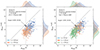 |
Fig. 1. Result of the BS and CenA flux excess analyses for our baseline volume-limited scenario, after scanning over the same parameter space in Eth and ψ as Auger (see text). Scatter plot of the CenA flux excess maximum significance versus the BS maximum significance obtained for 300 datasets using the JF+Planck (left) and the Sun+Planck (right) GMF models. Various coherence lenghts λc are considered for the GMF turbulent component (see legends). The values reported for Auger dataset at the ICRC 2019 are shown with a large black circle, the distributions of |


A first important remark is that the results show a very large dispersion both in  and
and  , which corresponds to orders of magnitude differences in the associated p-value or statistical significance. This is true even though the sources and their relative weight are all exactly the same in each case.
It is then interesting to compare the obtained values with those obtained with the Auger dataset, represented on Fig. 1 by a thick black circle. As can be seen from the probability distributions shown on the right and the top borders of the plot (in linear scale), the individual values of both  and
and  in the Auger data appear to be typical of the those found in our datasets, for both GMF models. Of course, whether the Auger data point is found on the lower end, middle or higher end of the simulated ranges of values depends on the assumed coherence length, λc, of the turbulent magnetic field component, but reasonable (in the sense of generically allowed) values of λc can be identified in each case to place the Auger values approximately in the middle of the simulated range (namely λc = 200 pc and 100 pc for the JF12+Planck and the Sun+Planck models respectively, see Fig. 1 for quantitative evaluation). However, what makes the simulation results interesting in this respect is that, on the other hand, the pair of values
  obtained with the Auger data is quite unusual in our simulations. As a matter of fact, for the Auger data,
  , which is related to the fact that the BS maximum in located in the sky at a position very close to that of CenA (∼2° away from each other, as reported at the ICRC 2019).
4.2. Direction of the most significant flux excess
We plotted in Fig. 2 the distribution of the locations of the BS maxima for the 300 datasets. The case of the JF+Planck model with λc = 200 pc is shown on the left, and that of the Sun+Planck model with λc = 100 pc on the right. As can be seen, the distributions obtained with the two GMF models are different, with a significant shift southwards of the distribution in the case of the Sun+Planck model. This is easily understood as a result of the strong demagnification of the sources in the Virgo cluster region in this case, as discussed below in more detail. We note however that the two distributions show a large overlap, notably in the region which happens to be where the Auger data indicate the most significant flux excess. The two models can thus not be distinguished on the sole basis of the prediction of the location of the BS maximum at this level of statistics.
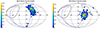 |
Fig. 2. Distribution of the locations of the BS maxima for the 300 datasets. The case of the JF+Planck model with λc = 200 pc (left) and the Sun+Planck model with λc = 100 pc (right) are shown. The colour scale represents the fraction of realisations for which the BS maximum is found in a given pixel of the sky (the pixel size correspond to Nside = 8 on these plots). The position of the CenA radio galaxy as well as the BS maximum location reported by Auger at the ICRC 2019 are shown with a red full circle and black star respectively (the two markers are practically on top of each other). The large red star shows the direction of the asymptotic BS maximum obtained with a 300 times larger simulated dataset (see text). |
The position of the (ICRC 2019) Auger BS maximum is shown on Fig. 2 as a black star near Cen A, represented by a red dot. For both GMF assumptions, that position appears rather uncommon in our simulations, although a position of the BS maximum close to that of Auger can indeed be obtained in some cases with both magnetic field models.
To better quantify the situation, we examined the distribution of the angular distances between the BS maxima found in our simulated datasets and i) the position of the BS maximum found in the Auger data (angular distance hereafter referred to as ΔθAuger), and ii) the position of the BS maximum that would be obtained asymptotically for the same astrophysical model with “infinite” statistics (hereafter referred to as Δθinf), as indicated with a red star in Fig. 2. To estimate the latter, we apply the BS analysis to a 300 times larger dataset obtained by putting together the 300 different realisations of the model under consideration. The cumulative distribution functions of ΔθAuger and Δθinf are shown in Fig. 3.
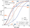 |
Fig. 3. Cummulative distribution, built over 300 datasets, of the angular distances Δθinf (full lines) and ΔθAuger (dashed lines) defined in Sect. 4.2. The cumulative functions obtained for the Sun+Planck GMF model with λc = 100 pc are shown in red, those for the JF12+Planck model with λc = 200 pc are shown in blue. |
As can be seen, concerning Δθinf, the curves are qualitatively and quantitatively similar, which can be understood as a consequence of the fact that both models have similar levels of anisotropy and BS maximum significance as the Auger data (see Fig. 1). One may thus estimate that a similar cumulative distribution function would also be obtained with the actual UHECRs themselves, that is if one had access to a large number of real UHECR data sets with the same statistics as Auger. Specifically, we find that 68% of the simulated datasets have their BS maximum within ∼17° and ∼20° of the asymptotic position, respectively for the Sun+Planck model with λc = 100 pc and for the JF12+Planck model with λc = 200 pc. These values may thus be considered as representative of the angular distance to be typically expected between the BS maximum direction currently reconstructed with the Auger data, and that which would be obtained at infinite statistics. Given this relatively large “angular resolution”, the very small angular distance between the direction of the Auger BS maximum and the direction of CenA should be considered with caution: according to our simulations, angular coincidences on scales lower than ∼15° cannot be considered meaningful at the current level of statistics.
The Δθinf cumulative distribution functions also allow us to quantify the compatibility of the simulated models with the Auger data, from the point of view of the direction of the BS maximum. Assuming that the actual UHECR phenomenology is exactly described by (one or the other of) our simulated models, one may wonder with what probability would a given data set with the Auger statistics have a BS maximum direction reconstructed (at least) as far away from the asymptotic direction as the actual Auger data are found to be. The answer can be read on Fig. 3. For the Sun+Planck model, the angular distance between the asymptotic BS maximum direction and the Auger data is ∼20°, and we find that ∼25% of the simulated data sets are at least as far away as this from the asymptotic direction. In the case of the JF12+Planck model, the angular distance to the Auger BS maximum direction is ∼25°, which is expected to be the case for ∼22% of the data sets. These numbers suggest that there is no strong contradictions from this point of view between the Auger data and the model expectations.
Conversely, starting with the position of the Auger BS maximum, one may wonder which fraction of the simulated models have their BS maximum direction within an angular distance corresponding to the abovementioned “angular resolutions”. This can be obtained from the ΔθAuger cumulative distribution functions shown as dashed lines in Fig. 3. We find that ∼38% of our datasets yield ΔθAuger < 17° for the Sun+Planck model, while ∼20% of our datasets yield ΔθAuger < 20° for the JF12+Planck models. These fractions remain sizeable, which again suggests that the BS maximum direction observed by Auger above 32 EeV is still marginally compatible with the simulated models, particularly for the Sun+Planck GMF model.
Finally, beyond the discussion of the BS maximum direction, it is worth nothing that datasets produced with the baseline model and the JF12+Planck GMF tend to predict high UHECR fluxes in the region of the sky near the Virgo cluster, seemingly in tension with the Auger observations. This property has important implications for the discussions below.
4.3. BS energy and angular scales
We also examined the distribution of the energy thresholds and angular scales at which the BS maxima were found, for the 300 realisations of the simulated models. The result is shown in Fig. 4 for both GMF models. We note that the distributions obtained for the two models are very similar. As can be seen, the BS maximum shows a clear tendency to be located on the boundaries of the parameter space, that is at the lowest values of the energy threshold and the largest angular scale. The same is true for the search of a flux excess in the direction of Cen A. This clearly suggests that higher significances could actually be found if one enlarged the range of scan parameters (see below). However, as Fig. 4 shows, even for an astrophysical scenario that does not favour the Auger values of the BS maximum parameters, these values or others similarly distant from the most likely ones for that scenario can be obtained from time to time. In such cases, finding the BS maximum away from the borders of the scanned parameter space may lead to the wrong impression that one does not need to extend the search further. Now, given the variance in the BS results at the current level of statistics, already shown in Figs. 1 and 2, it seems difficult to exclude the possibility that it is somewhat by chance that the parameters of the BS maximum of the current dataset are located inside the arbitrary limits of the predefined parameter range. For instance, for the models displayed in Fig. 4, ∼17% and ∼27% of the realisations, for the JF12+Planck and the Sun+Planck models respectively, have their BS maximum in the part of the parameters space delimited by the 2D interval Eth ≥ 35 EeV and ψ ≤ 28°. As a consequence the fact that the Auger BS maximum is not found at the lowest energies and largest angles of the explored parameter space cannot be used at this point to reject with high confidence level the type of scenarios that we consider.
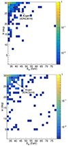 |
Fig. 4. Distribution of the threshold energy Eth and angular scale ψ of the BS maxima obtained after the analysis of 300 datasets assuming the same astrophysical models as in Fig. 2, the JF12+Planck model with λc = 200 pc (top panel), and the Sun+Planck model with λc = 100 pc (bottom panel). The colour scale represents the fraction of realisations for which the BS maximum is obtained in a given (Eth, ψ) bin. |
The above considerations clearly suggest that a significant increase in the UHECR statistics would be desirable. In the meantime, until larger datasets become available, it is advisable to extend the discussion, taking into account the intrinsic dispersion expected in the BS results for a given astrophysical model. In this respect, it is instructive to study in a more systematic way the evolution of the significance of the flux excesses as a function of the BS parameters (including outside the limited range used by Auger). This is what we do in the next two sections.
4.4. Evolution with the energy threshold
As discussed above, for a given astrophysical scenario there is a large dispersion in the expected values of the various quantities characterising the BS maximum in a dataset with the Auger statistics, namely the value of the maximum significance, the central direction of the corresponding flux excess, its energy threshold and its angular scale. This dispersion, however, also depends on the level of the true anisotropy associated with the model, that is the anisotropy that would be observed with infinite statistics. The larger the underlying anisotropy, the lower the dispersion (for a given UHECR statistics). For this reason, in the following study we choose the parameters of the model in such a way that the median of the values of the maximum significance in the simulated datasets,  , is roughly similar to the value reported by Auger (for comparable statistics).
We first examine the evolution of the BS maximum significance as a function of the energy threshold, Eth, for our baseline scenario with composition model A and the Sun+Planck GMF model with λc = 100 pc. We thus leave the angular scale unchanged, at ψ = 27°, and look for the most significant flux excess at each value of Eth from 32 to 80 EeV, with steps of 1 EeV. The result is shown on the top left panel of Fig. 5.
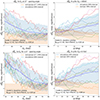 |
Fig. 5. Evolution of the BS maximum significance, |


As can been seen, the average value of the maximum significance,  , steadily decreases as the energy thresholds increases. This is due to the rapid decrease of the UHECR statistics as a function of energy, which is not compensated by significantly larger intrinsic anisotropies, since the energy evolution of the particle rigidities remains weak (see for instance the discussion in Lemoine & Waxman 2009) for the assumed composition, consistent with the measurements of Auger. However, when looking at individual realisations, the situation appears much more erratic. From almost any single simulated dataset with the current statistics, the general trend, although very clear on average, cannot really be guessed. In particular, some local maxima are often found for intermediate energy thresholds, which may then wrongly seem to reveal a preferred energy scale, while the global view on the 300 datasets clearly shows that this energy scale has nothing to do with the underlying astrophysical model, but only with the particular dataset under examination.
Following the discussion of the previous section, we also extended the range of the energy scan, from 8 EeV to 80 EeV, with steps of 1 EeV. The results are shown on the bottom left panel of Fig. 5. They confirm that larger values of  are obtained on average at lower energy thresholds.
It is interesting to note that the direction in the sky in which these maxima are found is very similar in the case of the wider scan, compared to the more restricted one. However, the dataset-to-dataset dispersion is smaller in the former case. This results from the fact that the anisotropies at lower energy generically have a larger significance, due to the larger statistics (even though they are not necessarily intrinsically stronger).
4.5. Evolution with the angular scale
We now repeat the analysis by varying the angular scale, ψ, instead, while keeping the energy threshold fixed. In the top-right panel of Fig. 5, we show the evolution of the maximum significance of a flux excess as a function ψ, in the case of Eth = 40 EeV and for the same data sets as above. Again, the average value of  shows a steady evolution with the angular scale, with larger values at larger smoothing angles. This is related to the predominance of the large scale structures of the source distribution in the observed anisotropy patterns. Tight UHECR multiplets from individual sources are essentially absent because of the large magnetic deflection (again consistent with the Auger composition measurements).
As for the energy evolution, we also extended the range of values of ψ, scanning up to 45 degrees (with 1-degree steps). The results are shown on the bottom right panel of Fig. 5. They confirm the indicated trend, but do not seem to provide additional information at the level of individual datasets, given the erratic behaviour of the excess significance as a function of ψ. We note that the results shown on Fig. 5 are perfectly in line with the findings of Sect. 4.3 and Fig. 4.
4.6. Distinct contributions to the flux excesses
It is instructive to examine the relative contribution of different sources to both the BS maximum and the Cen A region, at the energy and angular scales where a flux excess is the most significant. This cannot be done with actual data, of course, but we can easily extract from our simulated datasets which sources contribute the most, and at which level. In the case of our baseline scenario, the hierarchy of sources or sky regions contributing to the observed excesses are found to depend critically on the assumed GMF model, even when a fixed distribution of sources is considered. Here, we focus on the most significant excesses obtained with the BS analysis and in the direction of Cen A, regardless of the value of Eth or ψ at which they occur within the limits of the Auger scan.
The top-left panel of Fig. 6 is a scatter plot of two quantities computed for each of the 300 datasets simulated for the model under consideration: i) in abscissa, we show the fractional contribution of the dominant source, FTop1 = NTop1/Nobs, where Nobs is the total number of events in the angular window defining the BS maximum (same as Non in Eq. (1)), and NTop1 is the number of events coming from the source which contributes the most to this maximum; ii) in ordinate, we show the corresponding fractional contribution of the source Cen A, FCenA = NCenA/Nobs. The results obtained with our two reference GMF models are shown with different colours (see legend). The datasets located on the main diagonal correspond to datasets in which Cen A is indeed the dominant source in the BS maximum window, which is almost always the case when the Sun+Planck GMF model is used, and almost never the case with the JF12+Planck model (NB: M104, located slightly south of the Virgo cluster, is often the dominant source in that case, despite being more distant than Cen A, because of its much larger K-band luminosity, accordding to 2MRS). In any case, the contribution of the dominant source remains low, which indicates that the observed excess cannot be associated with a specific, individual source. Even when the dominant source is Cen A and the BS maximum is indeed located in a direction close to its position, its relative contribution has a median value between 5 and 10%, and never exceeds 20% of the flux in that direction.
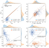 |
Fig. 6. Scatter plot of the contributions of different sources to the BS maximum, for 300 realisation of the baseline scenario, with the JF12+Planck GMF model (blue dots) or the Sun+Planck GMF model (orange dots). The corresponding probability distributions are shown along the top and right borders of the plots. Top left: fraction of events coming from Cen A vs. the fraction of events coming from the dominant source (i.e. the source contributing the most to the flux in the BS maximum angular window). Top right: fraction of events coming from either of the 5 dominant sources in the BS maximum window vs. the relative flux excess, r (see text) in that window (the dashed line displayed to guide the eye is of equation y = 0.5x). Bottom left: fraction of events in the BS maximum window coming any source in the Virgo association vs. the fraction of events coming from Cen A. Bottom right: same as bottom left, but for the excess in the Cen A direction instead of the BS maximum direction. The plot thus shows the fraction of events coming from any source in the Virgo association that are found in the angular window centered on Cen A for which a flux excess has the largest significance vs. the fraction of events in that window coming from Cen A. |
Similarly, it is interesting to investigate the contributions of dominant sources to the part of the UHECR flux in the BS maximum window that appears in excess of the isotropic expectation. For this, we define the flux excess ratio, r, as r = (Nobs − Nexp)/Nobs. In the top right panel of Fig. 6, we show the cumulated fraction of events in the top 5 sources as a function of this ratio, for the same 300+300 simulated datasets. The results, which are similar for both GFM models, show a flux excess between, say, one fifth and one half the isotropically expected flux. However, the contribution of the top 5 sources is always significantly lower than this, between ∼10% and ∼25%, and typically account for only about one half of the apparent excess (as represented by the dashed line on the plot).
Thus, it appears that the analysis of a flux excess cannot easily be used, by itself, to suggest one or even several dominantly contributing sources, but rather reflects a preferred direction in the sky where a large number of sources happen to contribute and build, together, a significant excess. Our simulations therefore suggest that this type of analyses should not be expected to pinpoint a particular source (at least with the current statistics), but could potentially constrain some general features of the source distribution. However, this can only be done if an assumption regarding the GMF can be made reliably. In particular, a key feature of the Auger dataset is the absence of a significant flux excess in the direction of the Virgo cluster, where many source candidates could be expected in principle. But this observation cannot be turned into a constraint on the UHECR source distribution until we have a reliable GMF model.
This is clearly demonstrated by the results shown in the two bottom panels of Fig. 6, where we compare the weight of the sources in the Virgo cluster (more precisely the Virgo association, as defined in Kourkchi & Tully 2017) with the weight of Cen A among the UHECR events in the angular window corresponding to the BS maximum (bottom left) or the Cen A excess (bottom right). The difference between the two GMF models is striking, but easily understood from our earlier remark that the Sun+Planck GMF model strongly demagnifies the sources in the Virgo direction. In this case, indeed, the contribution of these sources is always much smaller than that of Cen A, not only to the signal around Cen A, but also to the signal around the BS maximum, wherever it may be. It is typically between 1 and 5%, while Cen A contributes between 5 and 15%.
Conversely, the JF12+Planck GMF model does not strongly affect the flux of the UHECRs entering the Galaxy from directions around that of the Virgo association, so the corresponding sources contribute together a large fraction of the BS maximum signal, adding up to roughly one third of the events, while Cen A only contributes a few percent at most. In this case, of course, the BS maximum is indeed strongly “attracted” towards the direction of Virgo, as already shown in Fig. 2, which explains the small contribution of Cen A. Yet, even when considering the signal in the direction of Cen A itself (in the angular window corresponding to the most significant flux excess), Cen A as a source contributes between ∼3 and 10%, while the sources in the direction of Virgo contribute significantly more, namely between 15 and 25%. This larger contribution, however, is a collective effect of several sources, since Cen A generally remains the dominant source in this angular window even in the case of the JF12+Planck model.
4.7. Dependence on UHECR composition
Since the magnetic deflections depend on the rigidity of the nuclei, and thus at a given energy on their charge, the distribution of the arrival directions of the UHECRs could potentially provide a handle on their composition, independently of the measurement of the depth of the shower maxima in the atmosphere. In principle, specific signatures of the composition and its evolution with energy could thus be found in the associated evolution of the anisotropy patterns. As we did in Paper I with the evolution of the amplitude of the first two harmonics of the angular modulation (dipole and quadrupole), we show in Fig. 7 the evolution of the significance of the BS maximum as a function of the energy threshold, Eth, for two different composition models: model A (on the left), and model B (on the right), which is characterised by a larger maximum rigidity (see Table 2 of Paper I) and a weaker component of light nuclei (although this light component has a larger proton-to-helium ratio than in model A). In the case of Model B, the GMF coherence length is increased to 500 pc, to recover similar values of the average significances above 30 EeV as with model A, and thus allow comparison.
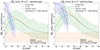 |
Fig. 7. Averaged Eth evolution of the BS maximum significance for different source composition models. The Eth evolution averaged over 300 datasets (setting ψ to 27°) is shown with a thick red line for the all particles dataset while the light (H+He) and heavier components are shown respectively in blue and green (the shaded areas show the 90% dispersion of the 300 datasets). The brown shaded area shows the 99% dispersion of isotropic datasets. For both panel, the baseline volume-limited catalogue and a 1 nG EGMF are assumed. The left panel shows the case of the source composition model A and the Sun+Planck GMF model with λc = 100 pc, and the right panel the case of model B and JF12+Planck model with λc = 500 pc. |
On Fig. 7, the red lines show the evolution of  , averaged over the 300 datasets for each model. Thus, the red line of the left panel is by definition the same as the dashed blue line on the bottom left panel of Fig. 5. As can be seen, models A and B show different behaviours, with a maximum significance reached at higher energy for model B, although still below 30 EeV (i.e. the limit of the Auger scan).
To better understand this general behaviour, it is interesting to isolate the “light component” (H and He) and the “heavy component” (all other nuclei) within the all-particle datasets, and to look at the energy evolution of  for these two components separately. The results are also shown on Fig. 7. The blue lines correspond to the light component, and the green ones to the heavy component. The shaded areas of the same colours show the 90%-interval over which the values for individual datasets fluctuate above and below the average.
For a given nuclear species, it is natural to expect an evolution of the corresponding values of  that is first increasing with energy, due to the proportional increase of the rigidities, and then reaching a maximum before decreasing as a result of the sharply decreasing statistics. The increasing part is missing on the plots for the light component, because of the low energy cutoff for H and He (although the “plateau” around the maximum is visible in the case of model B, which has a slightly higher maximum rigidity). Not surprisingly, the energy evolution of
  for the all-particle datasets depends on the UHECR composition through the balance between the light and heavy components (and at higher order on additional details of their composition). This is how complementary handles on the composition could be obtained, in principle, provided the statistics is large enough. The energy evolution of individual datasets with the current Auger statistics (depicted in Fig. 5) as well as our discussion of larger statistics datasets (see Sect. 8 below) suggest that a substantial increase of exposure would however be required for that purpose. Finally we note that on average, our simulations suggest that the most significant flux excesses are likely to be found with energy thresholds below 30 EeV for astrophysical models that account for the evolution of the composition implied by the Auger data.
5. Results of the likelihood analysis
We now turn to the results of the likelihood analysis on our simulated datasets for the same (baseline) scenarios as above. For the signal component of the likelihood fit, we focus on two catalogues: the 2MRS catalogue (used as a proxy to trace ordinary galaxies) and the starburst galaxy (SBG) catalogue (see Sect. 3.2).
5.1. Significance of the rejection of isotropy
In Fig. 8, we show the p-values corresponding to the maximum of the likelihood function for the SBG catalogue (in abscissa) and the 2MRS (in ordinate), for two different models of the GMF (Sun+Planck on the left, JF12+Planck on the right) and two different values of λc for each of them. Each data point corresponds to one of the 300 datasets simulated from our astrophysical scenarios. The values obtained with the Auger data are shown with a black circle.
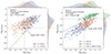 |
Fig. 8. p-values obtained after performing the likelihood analysis on our datasets. The logarithm of the p-value corresponding to the maximum likelihood obtained for the SBG catalogue (PSBG) catalogue is plotted against that obtained for 2MRS (P2MRS) for each dataset. The astrophysical model considered to build our datasets corresponds to model A, the baseline catalogue and a 1 nG EGMF. The values reported by Auger in Caccianiga et al. (2019) are shown with large black full circle. The individual distributions of the different quantities plotted are shown on top of the coordinate axis. The left panel shows the case of the Sun+Planck GMF model for two different values of the coherence length. The right panel shows the case of the JF12+Planck model. In this case we also show datasets produced after excluding galaxies from the Virgo association from the source catalogue (see legend). |
An important lesson can be drawn from the comparison of the results obtained with these two GMF models. It is indeed striking that the p-values obtained with the Sun+Planck model are (almost) always larger when correlating the datasets with the 2MRS catalogue than when correlating them with the SBG catalogue, whereas the exact opposite is true with the JF12+Planck catalogue. To make this easier to see, we plotted a diagonal dashed line corresponding to equal p-values for both source models: the data points are above that line on the left plot, and below it on the right plot. This fact should be welcome as a warning against premature interpretations of the Auger data as suggesting that a given catalogue somehow provides a better description of the UHECR sources than another. Although a typical realisation on the left panel of Fig. 8 appears very different from a typical realisation on the right panel from the point of view of the likelihood analysis, all the datasets shown on both panels are obtained with the exact same underlying astrophysical scenarios, that is with the very same sources, having the same intrinsic power and the same UHECR spectrum and composition at injection. Only the assumed GMF model is different.
The reason for the observed difference in the likelihood values is mostly related to the weight of the sources in the direction of the Virgo cluster, which happens to be strongly demagnified by the magnetic field configuration of the Sun+Planck GMF model. The SBG catalogue is thus more efficient in rejecting the isotropy hypothesis in that case, since the UHECR flux from the direction of Virgo is then much lower than what would be expected from the 2MRS catalogue if one simply assumes a gaussian blurring of the UHECR arrival directions, without systematic deflections, as in the Auger likelihood analysis.
The specific role of the Virgo cluster and its possible demagnification by the GMF is further seen on the right panel of Fig. 8, where we have added the result of the likelihood analysis for 300 additional datasets simulated with the JF+Planck GMF model, but from a modified version of our baseline scenario in which we removed the sources belonging to the Virgo cluster (based on their identification in Kourkchi & Tully 2017), as we also did for some scenarios in Paper I. In the non-modified case (red points), while the p-value obtained by Auger with the SBG catalogue is quite typical of the values obtained with our simulated datasets, their p-value is almost always much lower than that of Auger when performing the likelihood analysis with the 2MRS catalogue. However, when one removes the Virgo galaxies from the possible sources (green points), the resulting datasets are found to reject the isotropy hypothesis with larger significance when being analysed against the SBG catalogue than against the 2MRS catalogue, just as in the case of the Sun+Planck GMF model. This confirms the role of the Virgo cluster demagnification in the latter case. We also checked that the situation does not change, neither qualitatively nor quantitatively, when one removes the Virgo galaxies in the case of the Sun+Planck GMF model, as expected since the contribution of these galaxies is already strongly attenuated in that case.
We also note that, in these latter cases, a more significant rejection of the isotropy hypothesis is obtained when analysing the Auger data against the SBG catalogue despite the absence of CenA from this catalogue, even though CenA provides the strongest contribution to the flux excesses in our datasets. In the SBG model, excesses in the direction of the sky close to that of CenA are indeed accounted for by the expected contribution of NGC4945 and M83. Interestingly, these two sources are absent from the baseline source catalogue that we use to produced our datasets, since they do not pass the Ks-band luminosity cut applied to produce this volume limited catalogue.
5.2. Parameters of the maximum likelihood anisotropy signal
For each choice of a candidate catalogue, the likelihood analysis identifies the values of the parameters for which the largest correlation signal is obtained, namely faniso, which is the fraction of UHECRs that may be associated with sources in the catalogue, and θ, which is the angular scale over which the catalogue is to be smoothed (see Sect. 3.2). A scatter plot of the values obtained in the case of the SBG catalogue is given in Fig. 9, for 300 datasets simulated with the Sun+Planck GMF model (in red), and 300 datasets simulated with the JF12+Planck model (in blue). In the latter case, large values of the signal fraction, faniso, and large blurring angles, θ, are clearly preferred for the astrophysical model considered (with very small dependence on the assumed coherence length of the turbulent component of the GMF, in the range we considered). This is quite different from what was reported by Auger with their dataset, even though the p-values are of the same order as those found by Auger for this source catalogue, as shown above. On the other hand, lower values of both faniso and θ are found for the Sun+Planck model, with a majority of datasets in the range faniso ∼ 0.2 − 0.4 and θ ∼ 25° −35°. The values of faniso and θ are clearly correlated, with large values of faniso systematically associated with large smoothing angles. The likelihood function can thus occasionally yield values of faniso reaching 1 even though the intrinsic anisotropy of the simulated skymap under study is weak. Only a few datasets appear to lie within the 1σ ellipse reported in (Caccianiga et al. 2019).
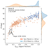 |
Fig. 9. Best-fit parameters obtained after performing the likelihood analysis for the SBG catalogue on our datasets. The value of faniso and θ allowing to maximize the likelihood for each dataset are plotted against each other for the astrophysical model considered in Fig. 8 and two GMF models (see legend). The 1σ ellipse reported in Caccianiga et al. (2019) from Auger data is shown. The individual distributions of the different quantities plotted are shown on top of the coordinate axis. |
Further discussion of this apparent mismatch requires consideration of the cosmic variance, this is of the fact that not all the sources above a given luminosity may contribute at all times, so variations depending on the specific subset of sources actually contributing to the current UHECR flux should also be explored. This is addressed in the next section.
Finally, we note that most datasets reject the isotropy hypothesis with the largest significance when the threshold energy, Eth, is set at the lowest values, that is close to the 32 EeV scan boundary. This is reminiscent of what we found for the BS and the Cen A flux excess analyses (cf. Figs. 4 and 5). However, there are indeed some datasets for which the largest significance is obtained for values of Eth close to 38 EeV or larger, in which case one might be tempted not to extend the scan range, although it could be relevant. Likewise, the Eth evolution of the p-value is found to have a large dataset-to-dataset variability at the current level of statistics, again reminiscent of what we found for the BS search (cf. Fig. 5).
6. Cosmic variance
To study the typical cosmic variance associated with our results, we adopt the mother catalogue approach presented in Sect. 2.2 and already used in Paper I. In this section, we restrict our discussions to source densities larger than 10−4 Mpc−3, which lead to better agreement with the observed level of anisotropy, at least for the considered range of extragalactic and Galactic magnetic field intensities. Lower source densities will be briefly discussed later.
6.1. Flux excesses from the blind search and around Cen A
As expected, the dispersion of the results for 300 datasets obtained with different realisations of the UHECR source distribution is larger than for datasets obtained with the baseline catalogue, both regarding the significance of the maximum flux excess and its location over the sky.
It is interesting to consider separately the realisations that include either Cen A, NGC4945 or M83 (or to impose one of these galaxies to be present among the sources). Indeed, this subset of realisations has a larger probability to produce a BS maximum localized close to that found by Auger. This is true for both GMF models, with a shift towards the direction of the Virgo cluster in the case of the JF12+Planck model (as anticipated from the results discussed in the previous sections). On Fig. 10, we show the cumulative distributions of the angular distance ΔθAuger defined in Sect. 4.2, in the case of model A and a 1 nG EGMF, using the mother catalogue approach with a source density of 10−3 Mpc−3. Separate distributions are shown for source realisations including either Cen A, NGC4945 or M83 (solid lines) and source realisations including none of those (dashed lines).
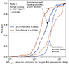 |
Fig. 10. Cumulative distributions of the angular distance ΔθAuger (see Sect. 4.2), obtained for the mother catalogue approach with model A, a source density of 10−3 Mpc−3 and a 1 nG EGMF. The red and blue curves correspond to different GMF models, as indicated. Separate distributions are shown for source realisations including either Cen A, NGC4945 or M83 (solid lines) and source realisations including none of those (dashed lines). |
In the former case, the median angular distance ΔθAuger is ∼17° for the Sun+Planck model, and ∼27° for the JF12+Planck model. The corresponding distribution of the BS maximum position over the sky is similar to that obtained above with the baseline catalogue. On the other hand, for the realisations without any of the quoted sources, this median angular distance is around 50° for both GMF models, with a lower significance of the BS maximum flux excess, on average. Thus, a position of the BS maximum in the close vicinity of the location of Cen A may be seen as somewhat favouring scenarios in which one of the quoted nearby sources is among the UHECR accelerators. However, it is important to keep in mind that this may be GMF model dependent, and that even when including these nearby sources, the expected dispersion in the BS maximum directions does not allow to draw strong conclusions from the direct comparison with the direction obtained from the Auger data at the current level of statistics, as already commented in Sect. 4.2.
Essentially the same results are obtained when lowering the source density to a 10−3.5 Mpc−3, except that the assumed coherence length of the GMF and/or the intensity of the EGMF have to be increased not to overshoot the observed significance of both the BS and the Cen A flux excess maxima, in particular for realisations in which at least one of the three above-mentioned nearby sources is present in the source distribution.
Finally, as expected, the realisation-to-realisation dispersion of the results also increases as the source density decreases.
6.2. Likelihood analysis
Allowing additional dataset-to-dateset fluctuations by taking into account the cosmic variance (i.e. drawing new sets of sources for each realisation) does not change the general finding that the reference catalogue leading to the most significant rejection of isotropy in the likelihood analysis depends on the assumed GMF model. This is shown on Fig. 11, where the same trend as in Fig. 8 can be seen: the datasets obtained with the JF12+Planck model are essentially located below the “equal rejection line”, while the opposite is true for the Sun+Planck model. However, the cosmic variance creates a few more outliers.
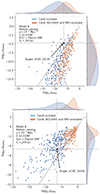 |
Fig. 11. Same as Fig. 8 but in the framework of the mother catalogue approach. The top panel shows the results of the likelihood analysis obtained for the JF12+Planck GMF model while the bottom panel shows those obtained for the Sun+Planck GMF model. On each plots, two categories of realisations are shown: source distributions in which the presence of CenA is imposed and source distributions which include neither CenA nor NGC4945 or M83. |
In Fig. 11, we also distinguish between realisations of the source catalogue in which the presence of Cen A is forced, and realisations in which neither CenA nor NGC4945 or M83 is present. In the case of the JF12+Planck GMF model, the presence of Cen A leads to somewhat smaller p-values in general (the same was observed by forcing one of the other two sources instead of Cen A). This could be expected, since the presence of a very nearby source tends to produce datasets with larger anisotropies on average (unless that source is strongly demagnified by the GMF). The presence of Cen A also appears to result more often in realisations for which PSBG < P2MRS, but such cases remain exceptional.
In the case of the Sun+Planck model, the impact of the presence of Cen A is much stronger, as can be clearly seen on Fig. 11. This is because in that case, the contribution of Cen A to the overall anisotropy is larger than in the case of the JF12+Planck model, because the Virgo cluster is anyway strongly demagnified (see Sect. 4.6 and Fig. 6). The vast majority of the realisations showing significant anisotropy (mostly those having Cen A as a source, but the same would be true for NGC4945 or M83) reject isotropy with a larger significance when using the SBG catalogue, as discussed in Sect. 5.
Regarding the distribution of the parameters of the likelihood maximum, faniso and θ, we find that including cosmic variance does not modify the main results, as they were presented in Fig. 9. Even in the most optimal cases, that is using the Sun+Planck model and imposing the presence of Cen A among the sources, only a handful of realisations (out of 300) fall within the 1σ ellipse extracted from the Auger data. Most realisations lead to parameters in the range faniso ∼ 0.2 − 0.4 and θ ∼ 20° −30°.
Finally, we found that forcing the galaxy NGC253 to be among the sources does not significantly modify any aspect of the above discussion. As noted in Sect. 5, when using the JF12+Planck GMF model, a more significant rejection of isotropy is obtained with the SBG catalogue for most realisations when the Virgo cluster sources are barred from UHECR sources.
7. Source distributions biased towards starburst or star-forming galaxies
7.1. Motivation
In this section, we further explore the role of the most nearby sources in shaping the UHECR angular distribution, and examine how a bias towards specific classes of sources could be used to reach a better agreement between the simulated datasets and the Auger data at the highest energies. For this case study, we impose among the UHECR sources a sample of nearby star-forming galaxies (SFGs), mostly originating from the HCN survey of Gao & Solomon (2004) and also used by the Fermi Collaboration in Ackermann et al. (2012) as a list of targeted sources to study the GeV γ-ray emission from SFGs. The main motivation for this analysis is that this sample, to which we added the Circinus galaxy located close to the Galactic plane, was used in the original Auger likelihood analysis to model the signal component in the “starburst galaxies (SBG) hypothesis”2. We note that essentially all of these sources are present in the 2MRS catalogue, and thus were randomly selected in some realisations of the UHECR source distribution in the “mother catalogue approach” discussed above. Some of them (notably, NGC253 and NGC1068) are also present in our baseline catalogue (provided that their K-band luminosity is large enough). In this section, however, they are all jointly present in all realisations.
7.2. SFG-biased catalogue generation
In addition to the above-mentioned SFG sample, we complete the effective source catalogues for this study by randomly picking sources from our volume-limited catalogue with the largest density, as we do in the mother catalogue approach. We assume that these sources inject UHECRs with the same energy spectrum and composition as in our model A, with an intrinsic luminosity proportional to their total infrared (IR) luminosity, LIR, which is expected to be a good proxy for the star formation rate of the galaxy. For the galaxies in the SFG sample, we use the IR luminosity given in Gao & Solomon (2004), corrected whenever needed to account for the more recent distance estimates that we are using (see Paper I). For the other sources, drawn from the mother catalogue, we randomly assign to them an IR luminosity by sampling the IR galaxy luminosity function obtained from the observations of the Spitzer satellite in Rodighiero et al. (2010).
In practice, we fix the density of the source catalogues built in this way by setting a threshold in the IR luminosity, above which we keep all the sources. This applies also to the galaxies in the SFG sample, which is assumed to include all the potential UHECR sources within 10 Mpc, once Circinus is added. The number of sources that need to be added from the mother catalogue to complete the sources beyond 10 Mpc depends on the chosen source density (or equivalently the chosen LIR threshold). For instance, a cut on LIR at 2 × 10¹⁰ L⊙ (where L⊙ is the IR luminosity of the Sun) corresponds to a source density of ≃ 10−3 Mpc−3 and allows to keep in particular M82, NGC253, M83, NGC4945, Circinus and NGC1068 from the initial SFG sample.
We also explore another possible type of biases in the UHECR source distribution, by implementing a second way to complete the source catalogue beyond 10 Mpc, namely by excluding a priori all the galaxies located inside large galaxy clusters with a mass larger than > 1014 M⊙, as identified in Kourkchi & Tully (2017). This is motivated, although in a very simplified way, by the possible lack or deficit of SFGs or SBGs in rich galaxy clusters (see, e.g., Guglielmo et al. 2015; Boselli et al. 2016).
7.3. Results
The p-values obtained for various models are displayed on the top panel of Fig. 12. When the Sun+Planck GMF model is used, the SFG-biased source model is found to produce similar results as reported above, without any significant improvement in the agreement between the simulated datasets and the Auger data. This is true both for the search of a flux excess (either through a blind search or in the direction of Cen A) and for the likelihood analysis. This confirms that NGC4945 and/or M83 can produce an anisotropy at intermediate angular scales that is similar to that produced by Cen A, and vice versa.
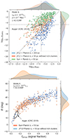 |
Fig. 12. Results of the likelihood analysis obtained for our special hypothesis on the source distribution of Sect. 7 (see text). The top panel is built as Fig. 8 and shows the cases of the JF12+Planck GMF (λc = 200 pc), the Sun+Planck GMF (λc = 50 pc) and a special case assuming the exclusion of galaxies members of nearby rich galaxy clusters from the source distribution and using JF12+Planck GMF (λc = 50 pc). On the bottom panel, similarly to Fig. 9, the faniso and θ parameters maximizing the likelihood analysis (for the SBG catalogue), for the last two cases shown on the top panel, are plotted against each other. |
In the case of the JF12+Planck model, a more significant rejection of isotropy is obtained when the SBGs are used as the underlying signal in the likelihood analysis, in the case when the second catalogue completion method is used, that is when galaxies in large galaxy clusters are excluded. This is again reminiscent of what was reported in Sect. 5.1. However, when the first completion method is used, although the proportion of the datasets that reject isotropy better when the likelihood analysis is performed with the SBG catalogue is found to be larger than in the case of non-biased datasets, this proportion remains below 25% for all the values of the LIR threshold that we considered.
Overall, for both GMF models and for the various cuts on the IR luminosity of the galaxies, no significant improvement is found regarding the similarity between a typical simulated datasets and the Auger data compared to what was obtained earlier with our baseline catalogue. Only a few realisations are found within the 1σ ellipse obtained from Auger data (see the bottom panel of Fig. 12).
7.4. General comment about the likelihood analysis results
The above results allow us to underline another important caveat regarding the likelihood analysis, in addition to the strong dependence of its results on the choice of a GMF model. Even though we forced the most nearby UHECRs sources, which are indeed those which determine or influence the most the resulting anisotropies, to be exactly the same as those used to model the signal component in the likelihood analysis (i.e. the SBG model used by Auger), the parameters reconstructed from the resulting datasets do not necessarily show a strong concordance with the underlying model. This is because the likelihood analysis, as constructed in Aab et al. (2018), assumes a simple gaussian blurring of the UHECR arrival directions around the SBG sources, which is not a realistic pattern to be expected from magnetic deflexions in the GMF. Even in the absence of significant magnification or demagnification, the GMF leads to systematic shifts of the UHECR image of given source over the sky, which depend both on its actual position and on the UHECR rigidity. Given the current lack of knowledge of the actual magnetic deflections, it is important to keep in mind that the values of the “signal fraction”, faniso, and angular scale, θ, providing the largest likelihood signal in such analyses should not be mistaken as an estimate of the fractional contribution of the dominant sources and of the typical magnetic deflection. Their meaning cannot be extrapolated beyond their technical role in the analysis, namely they are the set of parameters which allow to reject the isotropy hypothesis with the largest significance. As already discussed, caution is also required when it comes to the comparison of the p-values obtained for the various catalogues used to model the signal component.
8. Anisotropy expectations with larger datasets
As discussed in the previous sections, even when considering a wide range of generic astrophysical models and varying their main parameters, one does not seem to be able to find a satisfactory account of the entire set of information currently available about the UHECR anisotropies, which goes beyond the simple estimate of the significance of the rejection of an isotropy hypothesis, and includes the direction of the BS maximum, the amplitude of the anisotropy (see below) and its evolution with energy and angular scale. Although the Pierre Auger observatory has accumulated an unprecedented amount of good quality data at the highest energy, it is currently difficult to assess whether there is one or more key ingredients missing in the models, or whether the data are still subject to important statistical fluctuations that somehow blur the message or hide some important information that would only be accessible with still larger statistics. To explore this possibility and evaluate what could be gained from datasets containing several times more events, we examine in this section how the main anisotropy observables are expected to evolve as a function the accumulated statistics, at least in the framework of our generic models, and more specifically in the case of our baseline scenario, discussed through Sects. 4 and 5. To this end, we performed the BS analysis on datasets with statistics ranging from 1 to 10 times the Auger statistics reported at the ICRC 2019, which is our reference value throughout this paper (namely 42 500 events above 8 EeV, corresponding to an exposure of 101 400 km2 sr yr).
8.1. Energy dependence of the BS maximum significance
In Fig. 5, we had shown the evolution of the significance of the BS maximum flux excess,  , as a function of the energy threshold, Eth, for a given angular scale (namely ψ = 27°), and as a function of the angular scale for a given energy threshold (namely Eth = 40 EeV), where these fixed values of ψ and Eth are close to those corresponding to the BS maximum in the Auger dataset. These plots show a clear evolution of the values to be expected on average, but also that individual datasets with the statistics of Auger usually do not exhibit such an obvious trend, and may have a maximum at some particular energy or angular scale which is essentially fortuitous, and could thus be misleading if taken at face value to derive definite constraints about the underlying UHECR model. In Fig. 13, we show the same evolutions of
  , but for datasets 3 times (top panels) and 10 times (bottom panels) larger than the Auger dataset. The underlying model and the meaning of the individual curves and shaded areas are the same as in the bottom plots of Fig. 5.
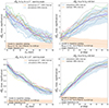 |
Fig. 13. Same as the bottom panel of Fig. 5, the top and bottom panels consider respectively statistics 3 and 10 times larger than that of Auger at ICRC 2019. |
As can be seen, in addition to the obvious increase of the significances due to the larger statistics, the energy and angular scale evolutions of  for the individual datasets appear less “noisy” when the size of the datasets increases, and are more and more representative of the average trends, from which interesting information could in principle be drawn. This is of course all the more true with ten times the Auger statistics.
8.2. Evolution of the BS maximum significance with statistics
Conversely, one can draw the evolution of  with the size of the dataset, for given values of the energy threshold and angular scale. This is done in Fig. 14, for an angular scale of 27° and 3 different values of the energy threshold, namely Eth = 10 EeV, 40 EeV and 80 EeV. The shaded areas show the intervals in which 68% of the 300 datasets are found in each case, and the size of the datasets, in abcissa, is expressed in units of the ICRC 2019 Auger statistics. The underlying astrophysical scenario assumes the energy spectrum and composition of model A, our baseline UHECR source catalogue, a 1 nG EGMF and the Sun+Planck GMF model with two different choices of the coherence length of the turbulent component. On the left plot, λc = 100 pc, for which the BS maximum and Cen A flux excesses of the simulated datasets have typical significances comparable to those reported by Auger (5.6σ and 5.1σ respectively), as seen in Fig. 1 (i.e., the Auger BS maximum significance above 32 EeV lies close to the median value obtained for 300 Auger-like datasets). On the right plot, λc = 200 pc, for which the Auger significances correspond to the higher end (positive fluctuations) of the simulated distribution.
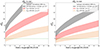 |
Fig. 14. Evolution of the significance of the BS maximum flux excess at an angular scale of 27° for 3 different values of the energy threshold, Eth = 10, 40 and 80 EeV, as a function of the size of the datasets, in units of the ICRC 2019 Auger statistics. The underlying astrophysical scenario is described in the text. The Sun+Planck GMF model is assumed, either with λc = 100 pc (on the left), or λc = 200 pc (on the right). The shaded areas show the 1σ interval around the average values of |

Of course, the values of all BS flux excess significances increase with the size of the dataset, but it is also interesting to note how the gap between the shaded areas increases, that is the differences between the BS maximum significances for different values of Eth are larger and larger. Thus, at least for the models under consideration, it becomes less and less likely to obtain a dataset for which the largest BS flux excess significance is found at high energy (say around 40 EeV, as in the Auger dataset) rather than at lower energy (∼10 EeV for model A or ∼20 EeV in the case of model B, as shown in Fig. 7). This is particularly true for the lower value of the coherence length (left plot) for which the expected level of anisotropy is indeed higher.
8.3. Flux excess ratio at the BS maximum
In Fig. 15, we show the evolution of the flux excess ratio, r = (Nobs − Nexp)/Nobs, associated with the BS maximum, for the same three values of Eth and the angular scale again fixed at 27°. As before, the shaded areas show the interval in which 68% of the realisations are found. The dashed lines show the asymptotic value of the flux excess, r, for the model under consideration, as would be obtained with datasets of “infinite” statistics. Comparing the two panels, one can see that the values of the maximum flux excess are on average larger for the smaller coherence length of the turbulent magnetic field, which follows from the corresponding higher level of anisotropy in that case.
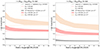 |
Fig. 15. Same as Fig. 14, for the evolution of the flux excess ratio r = (Nobs − Nexp)/Nobs. The dashed lines show the asymptotic values corresponding to datasets with infinite statistics. |
Unsurprisingly, the average maximum flux excesses observed in finite datasets are most of the time larger than the “true” (asymptotic) value. This is because the scanning procedure tends to always pick an upward fluctuation of the UHECR flux, in a region of the sky (probably) already characterized by an intrinsically larger flux than average. This overestimation effect is larger for smaller datasets and thus also larger for higher energy thresholds. For Eth = 10 EeV, the reconstructed value with the Auger statistics should be already within a few percent of what would be found with an arbitrarily large dataset. At Eth = 40 EeV, and even more so at Eth = 80 EeV, significantly larger statistics are required to better estimate the R ratio and characterize the actual anisotropy level. At Eth = 80 EeV, an order of magnitude larger dataset might be necessary to combine a large enough value of the anisotropy significance and a reliable estimate of the flux excess in the BS maximum region.
Another clear effect is the increase of the expected flux excess ratio as a function of Eth, even though the UHECR rigidity does not strongly evolve in this energy range, because of the composition change. This is in line with the larger expected anisotropies, as already discussed, and a natural consequence of the lower horizon distance of the UHECRs at higher energy, which reduces the number of sources. However, of course, a larger intrinsic anisotropy does not imply a larger significance, since the latter also depends on the size of the dataset. This is why, in the case of our model A, the values of  and r are clearly seen to evolve in opposite ways as a function of energy over the entire energy range above ∼10 EeV (or above ∼20 EeV for model B, as seen in Sect. 4.7).
Although the desirable gain in statistics requires important experimental efforts, with a new generation of either ground-based (Alvarez-Muniz et al. 2020; Hörandel et al. 2021) or space-based (Bertaina et al. 2019; Olinto et al. 2021) UHECR observatories, it is worth highlighting that increasing the statistics at the very end of the UHECR spectrum is particularly valuable, since the corresponding anisotropies are intrinsically larger at the highest energies, with a larger relative contribution of the brightest sources and a lower background from the more distant universe. The identification of the nature of the UHECR sources should thus greatly benefit from a significant gain in exposure, particularly in the highest energy part of the spectrum.
8.4. Direction of the BS maximum
Finally, Fig. 16 shows how the precision of the reconstruction of the BS maximum direction evolves with the size of the dataset. This is estimated from the difference between the reconstructed direction of each individual dataset at a given statistics and the direction obtained with an extremely large dataset (gathering 300 Auger-like datasets). On the plots, we show the angular distance, Δθinf, within which 68% of all datasets are found at the statistics considered, for a GMF coherence length of 100 pc (left) or 200 pc (right).
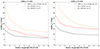 |
Fig. 16. Evolution with statistics of σ(Δθinf), the 68% upper limits of Δθinf (separation angle between the location of the BS maximum at a given statistics and the one that would be obtained with arbitrarily large statistics). The two same models as on Fig. 14 are considered. |
As expected, Δθinf evolves with the energy threshold and the statistics in the same way as the maximum significance  . As a result, in the case of model A, for a given exposure, the BS maximum location is found on average closer to its true position when Eth = 10 EeV, than for larger threshold. The same is true for model B, except that the cases for Eth = 10 EeV and Eth = 40 EeV appear closer to one another. For Eth = 80 EeV, an approximately 10× larger exposure is needed to reach the same precision on the position of the BS maximum as at 10 EeV. Regarding the influence of the GMF coherence length, one sees that the precision is higher for the smaller value of λc, due to the correspondingly higher intrinsic anisotropy.
From the quantitative point of view, the statistics of a dataset may be considered sufficient when the corresponding angular precision of the BS maximum reconstruction is small compared to its angular scale (here, ψ = 27°). At the highest energies, this requires a larger exposure. For instance, at Eth = 80 EeV, exposures of the order of 106 km2 sr yr (that is ∼10 times the current Auger statistics) are likely to be required to pinpoint the BS maximum location with an accuracy of 15–20°.
9. Comparison between the intermediate scale anisotropies at 8 EeV and above 32 EeV
As discussed above as well as in Paper I, our simulations show that there is potentially a lot information to be gathered from the evolution of the anisotropies with energy, both at large angular scales, with the amplitude and direction of the dipole, and at smaller angular scales, with the direction, significance and excess ratio of the BS maximum flux excess, or the evolution of the flux excess around a specific direction. While we do not have access to the full Auger dataset, and thus cannot develop this study with real data, the data made available by the Pierre Auger Collaboration on various occasions allow us to make a first comparison of the situation at Eth = 8 EeV (using the dataset released at the time of the publication of the Auger dipole anisotropy in Aab et al. (2017) and Eth > 32 EeV which we have discussed and compared to our simulations so far.
The dipole dataset includes UHECR events above 8 EeV and corresponds to a cumulated exposure of 76 800 km2 sr yr. Regrettably, the release does not include information about the energy of the listed events, so the full BS analysis cannot be performed on this dataset. We thus scanned only over the angular scales, with ψ ranging from 1° to 30° in steps of 1°, with a fixed value of Eth = 8 EeV. The most significant flux excess resulting from this analysis was found at the largest angular scale, namely ψ = 30°, with a significance  , in the direction (l = 267° ,b = −44° ) in Galactic coordinates. As for the targeted search of a flux excess in the direction of Cen A, the largest significance is found at ψ = 28°, with
  .
.
9.1. Comparison of the maximum significances in the Cen A direction
It is interesting, and perhaps very informative, that the flux excess in the direction of Cen A is much more significant above 32 EeV (namely  with the ICRC 2019 statistics) than when the threshold is set at 8 EeV. Of course, the possibility to scan over two parameters (ψ and Eth) instead of one leads to necessarily larger maximum significances. However, the dataset above 32 EeV is also much smaller than above 8 EeV, and the extra scanning dimension is not enough explain such a large difference, between 2.4σ and 5.1σ. To show this, we compare in Fig. 17 the two values
  and
and  obtained with our simulated datasets, for 3 different astrophysical models: the two models shown in Fig. 14, that is Model A with a GMF coherence length of 100 pc (blue dots) or 200 pc (red dots), and Model B with λc = 200 pc. We chose the Sun+Planck GMF model is all cases, since it leads to an overall better agreement with the Auger anisotropy measurements above 32 EeV when considering the baseline catalogue (see above), but similar conclusions are obtained with the JF12+Planck model. The Auger data are represented by a black circle, which appears very far from the typical location of the simulated datasets in this 2D plot. Indeed, even though the significance of the maximum flux excess at Eth = 8 EeV is often lower than the signifance above 32 EeV (datapoints below the diagonal in Fig. 17), the difference is almost never as large as in the case of the Auger data. (NB: in the simulated datasets, we reproduced the same exposure difference as in the available Auger data.)
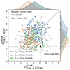 |
Fig. 17. Scatter plot of the maximum significances of a flux excess in the direction of Cen A with a fixed energy threshold at Eth = 8 EeV (in ordinate) and with a scan over Eth > 32 EeV. The different colours correspond to different underlying astrophysical scenarios, as indicated on the plot. The two values of σmax obtained with the Auger data are indicated by the black dot. |
The case of Model B with λc = 200 pc appears slightly more favourable, with the Auger data around Cen A corresponding to a moderate downward fluctuation of the low energy flux and moderate upward fluctuation at high energy. This can be understood as a consequence of the different energy evolution of average maximum significance between 8 EeV and 32 EeV for model A and model B, as already observed in Fig. 7. However, these data would still appear quite unsual for such models, when both energy ranges are considered together. This shows once more the interest of examining the UHECR data globally, with the entire set of observables including their evolution with energy, as already emphasized in Paper I.
Incidentally, we note that, in the case of Model A, the larger value of λc (red dots) is also the one which better reproduces the value of the dipole amplitude and its energy evolution (see Paper I). In the framework of the simulated scenarios, this would thus tend to favour an interpretation of the apparent mismatch between  and
and  according to which the later benefits from an upward fluctuation, rather than the opposite.
9.2. Comparison of the maximum significances of the BS maximum flux excesses
We extended the study to the comparision between the significances of the BS (blind, i.e. non targeted search) maximum flux excess at Eth = 8 EeV and above 32 EeV. The results, shown in Fig. 18, confirm that the Auger dataset is much less atypical from this point of view, compared to the simulated datasets. In the case of Model A with λc = 200 pc, many realisations of the scenario lead to values of  and
and  similar to those obtained with the Auger data. It is also interesting to note that lower values of the GMF coherence length are again disfavoured, at least for the models under study. Indeed, for these values (blue dots in Fig. 18), although the significance of the maximum flux excess above 32 EeV appears on average very similar to the Auger value, the significance at 8 EeV is almost always much larger. From a general point of view, a lower value of λc allows the gain in statistics at low energy to be translated into a larger gain in significance, despite the (moderately) lower magnetic rigidity and larger number of sources (more distant horizon).
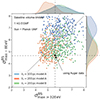 |
Fig. 18. Same as Fig. 17, but for a blind search (BS) of the maximum flux excess, instead of targeted search in the direction of Cen A (see text). |
9.3. Energy evolution of the flux excess significance at the position of the BS maximum at 8 EeV
In the last two sections, we saw that the magnitude of the Auger flux excesses at 8 EeV and above 32 EeV is well reproduced by our simulations if one does not specify a given direction in sky, but is strongly different from the expectations of our generic models when the search is performed in the specific direction of Cen A. Since the region very close to Cen A does not play such a prominent role in our simulations as it appears to be the case in the Auger data above 32 EeV, it is interesting to address a more general question, focusing not on a predefined direction in the sky, but on a direction that is identified from the datasets themselves, independently of any preconception, namely the direction of the BS maximum at low energy.
We applied this idea to the same simulated datasets as above, with the following procedure. First, we performed the BS maximum study with Eth = 8 EeV for each individual dataset, determining both its significance and direction. Then, we performed a targeted search for a flux excess above 32 EeV in the very direction where the maximum significance was found, scanning over Eth and the angular scale, ψ, but not over the positions in the sky. We recorded the largest significance,  . The results are shown in Fig. 19, for the same three models as above, through a scatter plot of the three times 300 realisations of
  versus
  . The position of the Auger data in this plot is indicated by a black dot. To obtain it, we used the dataset of Abreu et al. (2022) up to a total exposure of the ICRC 2019 (∼101 400 km2 sr yr) to match our simulated dataset statistics, and found a maximum significance of the targeted search of
  .
.
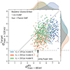 |
Fig. 19. Scatter plot of the maximum significances for Eth > 32 EeV of the flux excess in the direction of the BS maximum at 8 EeV, |


The result is particularly striking, as it shows how exceptional the situation of the Auger data is. Unsurprisingly, the significance of the maximum flux excess above 32 EeV is generally smaller than what it was at Eth = 8 EeV, since i) the dataset is smaller, and ii) the targeted position was optimized by the BS at 8 EeV, and not allowed to vary anymore. It thus usually corresponds to an upward fluctuation of an underlying high flux region, which has no reason to be also present with a similar fluctuation in the high-energy data (which amount to a negligible fraction of the dataset above 8 EeV, given the rapid decrease of the spectrum). However, in the case of the Auger data, the significance of the flux excess above 32 EeV appears to have largely collapsed at the position where it was maximum at Eth = 8 EeV. Indeed, between the two Auger datasets, the significance dropped from 4.7σ to 1.7σ, much more than for the vast majority of the simulated datasets.
From Fig. 19, one may conclude that, among the generic models that we studied, the Auger data would be best understood as very negative fluctuations of the flux expected above 32 EeV in the direction of the maximum flux excess at 8 EeV, with a remote preference for model A and λc = 200 pc, which is the least incompatible with the observations. However, the strong apparent disagreement between the data and our simulations on this particular exercise allows to speculate that the actual UHECR phenomenology in this energy range may be fundamentally different from the simulated one. Indeed, the expectation that a genuine and significant flux excess in some direction at low energy remains measurably significant at high energy is a natural and quite generic expectation in the framework of low proton-Emax scenarios, with the additional assumption that all sources emit UHECRs with roughly similar compositions and energy spectra. In such models, the average UHECR rigidity evolves slowly with energy, so the regions of the sky corresponding to larger UHECR fluxes remain the same in various energy ranges. There is no clear mechanism, in such a framework, that would allow a significantly larger flux in a given region to rapidly disappear in a neighbouring energy range.
Therefore, we are left with the following possibilities: i) the signal at low energy is a strong positive fluctuation of the UHECR flux, in the direction of the maximum that we obtained, namely (l = 267, b = −44); ii) the low maximum significance of the corresponding excess above 32 EeV corresponds to a strong negative fluctuation of the UHECR flux in this direction; iii) a contribution to the UHECR flux that is responsible for the position of the BS maximum excess location at 8 EeV simply vanishes at high energy.
The first possibility is interesting in the perspective of our study (both this paper and Paper I), as it would tend to reconcile the generic type of models that we are analysing with the Auger data, not only from the point of view of the BS flux excess maximum at 8 EeV, but also from the point of view of the dipole direction, which was discussed in Paper I. Indeed, while the direction in which the Auger data have the most significant flux excess at a threshold energy of 8 EeV is in the vicinity of the Fornax cluster, which to leads to a somewhat larger flux than average in our simulations, this excess is never dominant in essentially all of our simulated datasets, whatever the GMF model and the other astrophysical parameters. Only a strong upward fluctuation could change this situation. But it is also worth noting that the presence of this particular flux excess in the Auger data at above 8 EeV has necessarily a direct influence on the direction where a dipolar modulation is found in this same energy range, namely in the two energy bins from 8 EeV to 16 EeV and from 16 EeV to 32 EeV. The same upward fluctuation that would produce a BS maximum flux excess where Auger finds it would also drag the direction of the dipolar modulation southwards in Galactic coordinate, thereby reducing the disagreement with our simulations on this aspect (see Paper I). However, the fact that a fluctuation of the required amplitude never occurred in our simulations (with 300 datasets for each set of parameters) suggests that this possibility, although interesting for the mentioned reasons, remains quite unlikely.
Regarding the second possibility, namely a downward fluctuation above 32 EeV, only additional data may provide useful insight. If the low flux excess significance is confirmed, then the third possibility will become likely, and all the more interesting, as it would clearly would represent a very important astrophysical information. Such a rapid decrease of the significance of a flux excess in a given direction would indeed be direct evidence for a strong departure from the generic expectations for UHECR models based on standard candle sources, or even suggest the existence of a UHECR component vanishing between Eth = 8 EeV and Eth = 32 EeV. It would certainly be helpful for this discussion to have access to the full Auger dataset, as it would increase the statistics by more than 50% with respect to the dipole dataset, and allow to discuss the energy evolution between 8 and 32 EeV, thereby bringing additional constraints. This is further discussed in the next and final section.
10. Summary and discussion
In this paper, we extended the general study of the UHECRs anisotropies initiated in Paper I by confronting the available observational data with a wide range of simulated datasets based on the generic assumption that the distribution of the UHECRs sources in the universe follows on average the distribution of galaxies, possibly with some bias in favour or against specific classes of sources. In this second part, we focused on small and intermediate angular scales, exploring anisotropies through different types of analyses already used by the Auger and TA Collaborations, namely the search of a flux excess either in any direction (“blind search”, or BS) or in a predefined direction (e.g., Cen A or, as a new type of study, in the direction of the maximum flux excess in a different energy range), as well as the search for similarities between the distribution of UHECRs and some catalogues of sources, through the so-called likelihood analysis.
In addition to the above-mentioned assumptions regarding the UHECR source distribution, we explored different scenarios varying several astrophysical parameters, namely the composition and the energy spectrum of the UHECRs at their source, the source density, the typical strength of the extragalactic magnetic field, the structure of the Galactic magnetic fields and the coherence length of its turbulent component. With simulated hundreds of datasets for each scenario, which allowed us to investigate the uncertainties associated with both the statistical fluctuations and the cosmic variance.
10.1. BS and targeted flux excess
Concerning the search of a flux excess in the UHECR skymap, we found that the values derived from the Auger data for both the maximum significance of a blind search and the maximum significance of a flux excess in the direction of Cen A were individually relatively easy to reproduce with our baseline simulations (see Sect. 3.1.1). Concerning the direction of the BS maximum, the dispersion found among our simulated datasets, which reproduce the anisotropy level observed by Auger, suggests that its “true” position cannot be currently estimated with a resolution better than ∼15 − 20°. This implies that the very close proximity between the Auger BS maximum and the position of the radiogalaxy CenA is not astrophysically meaningful at this point and that this observation needs to be strengthened with significantly larger exposure measurements. Moreover, the BS maximum direction observed by Auger lies in the periphery of the distributions obtained with our simulated datasets and thus appears marginally compatible with the expectation from our astrophysical models. In the case of the JF12+Planck GMF model and the baseline catalogue, the flux excesses expected in the region of the sky near the Virgo cluster are however more in tension with the data and play an important role in the outcome of the likelihood analysis.
For a given source catalogue, the fractional contributions of the various sources to the BS maximum flux excess depend on the GMF model assumed. For choices of the parameters that lead to a BS maximum significance comparable to that of Auger, the corresponding excess can be attributed to the cumulative contribution of a sizable number of sources, with the brightest source providing only a rather modest contribution to the relative flux excess, r (cf. Fig. 6). In the case of the JF12+Planck GMF model a strong contribution of the sources in Virgo cluster and the nearby structures (see also Ding et al. 2021) is expected from our simulations, while it is not the case for the Sun+Planck GMF model as a result of a strong magnetic demagnification of the Virgo region. When using our baseline catalogue and the Sun+Planck GMF model, we find that Cen A is in general the source contributing the most to the BS maximum flux excess, even though its central direction remains in general at an angular distance of the order of ∼20° (median value) from the actual position of that Galaxy. This result provides an important reminder that the position of the maximum flux excess (even with very large statistics, such as obtained by combining our 300 Auger-like simulated datasets) is not necessarily located very close to the celestial position of the most contributing source.
10.2. Likelihood analysis
One of the most striking features of the Auger dataset at the highest energy is the absence of any notable flux excess in the region of Virgo cluster. This absence probably has a strong influence on the fact that the SBG catalogue is preferred when the likelihood analysis is performed on the Auger data, as discussed in Sect. 5. This feature can be either at odds or in line with our simulations when the UHECR source distribution is assumed to follow that of the galaxies, depending on which GMF model is assumed to produce the simulated datasets.
In the case of the JF12+Planck GMF model, our baseline simulated datasets predict a strong contribution from the Virgo region, which results in a direction of the BS maximum flux excess that is systematically shifted northwards in Galactic coordinates with respect to that obtained with the Auger data, and to a more significant rejection of isotropy based on the likelihood analysis with the 2MRS catalogue hypothesis than with the SBG catalogue. On the other, hand, when using the Sun+Planck GMF, the magnetic demagnification of the Virgo region results in the opposite outcome for the likelihood analysis, namely a more significant rejection of isotropy with the SBG source model and a BS maximum flux excess shifted in most case to lower Galactic latitudes.
To obtain the same outcome with the JF+Planck GMF model, one would have to make some additional hypotheses regarding the source distribution, such as assuming that large galaxy clusters, thus in particular the Virgo cluster, are much weaker sources of UHECRs than regions with less concentrated galaxies. In Sect. 5, we explored such a bias in a rather extreme form, assuming that such dense environments are simply devoid of any UHECR sources. More moderate versions of this bias could be justified on the basis of astrophysical scenarios where a high star formation rate plays an important role in the origin of UHECRs, since rich galaxy clusters tend to be significantly less active in this respect. Another justification could involve the trapping and destruction of UHECR nuclei in the environment of large galaxy clusters as discussed in detail in Kotera et al. (2009), Armengaud et al. (2005). The latter could represent a viable possibility at the highest energies, say above 32 EeV, where the UHECRs responsible for the anisotropies are expected to be dominated by CNO and heavier nuclei in our models. It is however less likely to apply as much to protons and He nuclei, since they have much larger photo-nuclear interaction lengths and should thus be less affected. Their presence around 8 EeV, that is in the energy range where the dipolar modulation is most significant in the Auger data, should then still attract the dipole direction northwards, far from where it is actually observed by Auger (see the corresponding discussion in Paper I).
It has also been argued in Kim et al. (2019) that the filamentary structure of the EGMF in the nearby universe could be responsible for the systematic deflection of UHECRs originating from the Virgo cluster towards completely different apparent arrival directions. Such a scenario was invoked to justify a potential major contribution of the UHECR events from the Virgo cluster to the TA hotspot (Abbasi et al. 2014; Kim et al. 2021). Such potential effects cannot be captured by our simulations, since we assume a homogeneous EGMF.
Undoubtedly, in the quest for the origin of UHECRs, it will be important to understand whether the lack of an excess of events in the region of the Virgo cluster is due to a bias in the distribution of UHECR sources with respect to that of the galaxies, irrespective of their membership of large clusters, or to the spatial distribution of the GMF and/or the EGMF. This will require better constraints on the intensity and structure of the GMF, which currently remain very uncertain (see in particular recent discussions in Unger & Farrar 2017, 2019; Boulanger et al. 2018), and of the EGMF (see e.g., Heald et al. 2020; Beck 2008 and references therein), as well as additional theoretical progress on the modeling of potential UHECR sources and their environment. In the current stage of knowledge, our results suggest that the greatest caution should be used when interpreting the differences in the p-values for isotropy rejection that are obtained with different catalogues to model the UHECR signal component.
Moreover, in Sect. 7.2, we used source catalogues obtained by forcing the presence of the SFGs used to model the signal component in Aab et al. (2018) and found no significant improvement in the comparison between the data and the simulations in the framework of the likelihood analysis. This is true both from the point of view of the preferred model for the signal and the value of the signal fraction, faniso, and angular scale, θ. This result allowed us to emphasize a well-known shortcoming of the likelihood analysis, which relies on a simple Gaussian blurring to model the deflection of the UHECRs, discarding the systematic shifts of the image of the sources resulting from the crossing of the GMF (not mentioning possible magnification/demagnification effects). In the context of this simplifying hypothesis, even when the sources used to model the signal component are included in the source catalogue used to produce the simulated datasets, the values of faniso and θ maximizing the likelihood should not be considered as an estimate of meaningful physical parameters, but rather as what they merely are, namely the set of parameters allowing to reject isotropy with the largest significance.
10.3. UHECR source density
Most of the models discussed in this paper assumed relatively large source densities, typically ≳10−3.5 Mpc−3. This is because we found that for typical values of the EGMF of the order of 1 nG and GMF coherence lengths varying from 50 pc to 500 pc, source densities as large as a few 10−3 Mpc−3 are indeed acceptable from the point of view of the resulting significance of the associated UHECR anisotropy, as estimated with the Auger statistic. In particular, similar values as with the Auger data can then easily be obtained for the significance of the BS maximum flux excess as well as for the likelihood p-values. This does not mean, however, that lower source densities should be considered as disfavoured. Indeed, because the cosmic variance is larger in this case, some realisations of the lower density scenarios can result in simulated datasets with anisotropy levels similar to those found with our baseline catalogue. This is mostly the case when the closest UHECR source happens to be rather distant compared to what is found for a typical realisation. On the other hand, for realisations combining a low source density (say 10−4 Mpc−3 or lower) and a nearby closest source (e.g. as close as Cen A), significantly larger EGMF (especially if those are confined to the local Universe) must be invoked to keep the level of anisotropy as low as observed.
In the absence of strong constraints on the structure and intensity of the EGMF in the local Universe, UHECR models assuming a dominant contribution of very few sources are viable in principle. Such scenarios could be favoured in a context where the production of UHECRs is related to the presence of relatively rare objects, such as jetted AGNs. In that case, the source catalogue compiled by van Velzen et al. (2012) is interesting to use since its radio luminosity cut provides a volume-limited catalogue up to ∼150 Mpc (with a source density of ∼10−5 Mpc−3) from which to infer the distribution of potential sources as well as their associated UHECR luminosities. It suggests, in particular, that nearby sources such as CenA and/or FornaxA and/or M87 could make a considerable contribution to the overall UHECR flux at the highest energy. Although located at ∼230 Mpc away from Earth, Cygnus A has such a large intrinsic (radio) luminosity that it could also provide a strong contribution to the observed flux (but then only say below ∼20 EeV because of energy losses). Some scenarios assuming a dominant contribution of one or several of these nearby sources have recently been considered (see e.g., de Oliveira & de Souza 2023; Matthews et al. 2018; Mollerach & Roulet 2019). It will be interesting to investigate whether such models can provide a satisfactory account of the various aspects of the UHECR data, beyond one specific observable, for instance whether they can reproduce not only the position, but also the amplitude of the dipolar modulation (e.g. without overproducing the quadripolar modulation), as well as the overall level of anisotropy at high energy, without too much fine tuning of the dominant source(s) emission (spectral shape, composition, maximum energy, beaming, time evolution) and/or of the local universe magnetic field configuration. In parallel, further theoretical work on the acceleration of UHECRs in this type of sources will be welcome, as well as new progress on theoretical and observational constraints on the local universe magnetic field structure.
10.4. Energy evolution
Throughout this paper, we emphasized the importance of investigating the energy and angular evolution of the anisotropy signal, to reinforce and provide new constraints on the astrophysical models. Some of the existing, but currently non public data may already provide interesting information. To push this type of investigations described above up to, say, 80 EeV, a significant increase in statistics will be necessary. The levels of anisotropy (defined by the relative flux excess, r, introduced in Sects. 4.6 and 8) that this will allow to characterize are expected to be larger than those found at lower energy, because of the reduced UHECR horizon and the larger relative contribution of the nearby sources. Therefore, they may be expected to provide new constraints on the sources of UHECRs. Alternatively, as discussed in Paper I, interesting constraints could be provided by the study of the light component (if any) above, say 20 EeV, where the horizon of He nuclei significantly drops and becomes restricted to the local universe, due to photo-disintegration interactions. This will be most valuable if the H/He abundance ratio is low at this energy, and if the separation from the heavier nuclei is efficient.
In the previous section, we carried out a preliminary discussion of the energy evolution of the anisotropy below 32 EeV, using the Auger dataset published in the “dipole paper” (Aab et al. 2017). The examination of the Auger data above 8 EeV, shows that the flux excess in the direction of CenA has a maximum significance of ∼2.4 well below the one found scanning the data above 32 EeV. This energy evolution is in tension with the predictions of our simulations, in particular when our composition model A is used.
Moreover, a BS maximum flux excess at (l = 266°, b = −44°), somewhat above the direction of the Fornax cluster and south of where the dipole direction is found with this same dataset, is obtained. The existence of this higher-flux region clearly drags the direction of the observed dipolar component of the anisotropy towards the position where it is found in the 8–16 EeV energy bin, and can be seen as, at least partly, responsible for the discrepancy between the Auger data and our simulated datasets (see Paper I)3. When one compares with the UHECR sky seen by Auger above 32 EeV, it is striking that the flux excess in this region has essentially disappeared.
It would be very interesting to know if the situation of this broad region is continuously evolving with energy, from which one may hope to see an astrophysically meaningful pattern emerge. Indeed, if one were to take at face value the results of Sect. 9.3, discarding for the sake of exploration the possibility of strong statistical fluctuations, one would be led to formulate some assumptions about possible amendments that would need to be made to the investigated scenarios. Among the possibilities, on may speculate that an extended Galactic component still contributes to the UHECR flux above the ankle, and then disappears. This would probably imply an extended magnetic halo able to confine particles at a higher energy that usually assumed, with additional consequences concerning the deflections of extragalactic UHECRs in the GMF. Another possibility could be the existence of a strong (possibly nearby) source with a particularly low energy cutoff. This would probably be more natural in the context of scenarios in which very few sources provide a large fraction of the flux observed above the ankle.
Although the potential implications of what would be a clear and consistent modification of the UHECR sky map as a function of energy are very interesting, it is important to stress that, at the moment, such a finding would clearly be a posteriori. It would thus be dangerous to draw any strong conclusion from it at this stage, even if a clear pattern, with a smooth and definite evolution with energy would appear to be present in the data. However, if such a pattern were to be observed in entirely independent datasets and could thus be considered a real, significant feature of the UHECR sky, then it could bear genuine astrophysical meaning, likely to shed long awaited light on the origin of (at least some of) the UHECRs. This is unfortunately not the case of the mere assessment of anisotropies, which by themselves do not tell us much about this origin and cannot be used in practice to constrain the proposed source models efficiently, especially in the absence of a reliable GMF model, as the results of the present paper show.
Given the a posteriori nature of such a discussion, it is likely that the current data will not allow to assess a behaviour such as the one sketched above (or other meaningful ones) with a high level of confidence. However, the public release of the currently collected data would allow the larger scientific community to push further such investigations. We understand the perceived risk of multiplying independent searches, compromising the statistical power of each given analysis. But since, to the best of our knowledge, the data have never been blinded within the Auger and TA Collaborations, this is true anyway, whether the data are released or not. From this point of view, whether astrophysically meaningful patterns are present or not in the data, finding hints of them earlier can only be beneficial to the community in general, and allow meaningful future searches on independent datasets.
10.5. Final comments
In conclusion, the class of models that we have investigated in this paper and in Paper I appeared to have difficulties to globally reproduce the Auger observations above 8 EeV. While, the observed anisotropy levels and significances are relatively easy to match by adjusting the free astrophysical parameters at our disposal (in particular the EGMF intensity of the GMF coherence length), some observed characteristics of the data, essentially related to the location of the predicted flux excesses and possibly to the energy evolution of the various anisotropy signals, proved to be much more challenging to reproduce even after taking into account the cosmic variance and statistical fluctuations of the simulated datasets. These discrepancies, which were also stated in Paper I regarding the direction of the dipolar modulation, may call for a reconsideration of some of the key hypotheses underlying the astrophysical scenarios that we investigated, which rely on standard candle sources (at least in terms of spectral shape, composition and maximum energy) following the distribution of Galaxies and forming a single extragalactic component fully dominant above the ankle.
Unfortunately, as we have shown, the analysis of specific anisotropy signals can be very different depending on the assumed model of the GMF. In the absence of sufficiently strong constraints regarding this key ingredient of any modeling of the UHECR sky, it is thus difficult to judge to what extent the above-mentioned discrepancies are indicative of explicit failures of particular astrophysical assumptions, and how they could be used to make significant progress in the quest of the origin of UHECRs. As stressed all along these two companion papers, a better understanding and knowledge of cosmic magnetic fields appears crucial to push further the endeavour of deciphering the UHECR sky, which should go in parallel with improving the theoretical modeling of potential UHECR sources (in particular but not only from the point of view of the expected composition), which should help to narrow down the a priori range of the remaining astrophysical free parameters.
Finally concerning UHECR data themselves, given the relatively low level of anisotropies in the UHECR sky, as currently measured by the existing experiments, it appears unavoidable, if significant progress is to be made in this important field at the heart of high-energy astrophysics and astroparticle physics, that a new generation of detectors be constructed with much larger statistics and/or full sky coverage (Coleman et al. 2023).
Note added in proof. During the review process of the paper, new magnetic field models have been proposed (Unger & Farrar 2023, referred to as the UF23 model), as an update of the JF12+Planck model that we used. We implemented these new models in our codes and found that the results obtained with the various versions proposed do not modify significantly the results presented here. In particular, it is confirmed that one key property of the GMF model is related to the possible magnification or demagnification of the region of the sky of the Virgo cluster, which directly impacts the position of the expected dipole, the amplitude of the quadrupole, as well as the interpretation of the outcome of the likelihood analysis and the position of the hottest spot at high energy. For reference, we show in Fig. 20 the magnification factor of the Virgo region as a function of rigidity, for the two GMF models used in this paper (JF12+Planck and Sun+Planck) as well as 5 of the 8 newly released models (the other 3 are omitted for clarity, but very similar to the so-called “nebCor” model). As can be seen, all the new models are strongly demagnifying Virgo up to a rigidity of ∼1019 V, except the so-called “twistX” version, which shows an earlier recovery. This is in sharp contrast with the original JF12+Planck model, and more similar to the Sun+Planck model. As a result, most of the new models, except twistX, favour an interpretation of the likelihood analysis similar to that obtained with the Sun+Planck model. In sum, the new models do not modify our main conclusions, in particular about the importance of examining the evolution of the anisotropy signal with energy, and further underline that the uncertainty on the GMF remains a major limitation for the astrophysical interpretation of the UHECR skymaps.
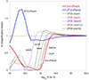 |
Fig. 20. Magnification factors of the Virgo region (∼15 degrees around the centre) as a function of particle rigidity, obtained with the different magnetic field models, as indicated. Five versions of the UF23 GMF model are shown (see Unger & Farrar 2023). |
The most important sources of this sample were also present (and had a dominant contribution to the signal component) in the subsequent iterations of the likelihood analysis performed by the Auger Collaboration, based either on the Becker et al. (2009) or the Lunardini et al. (2019) samples.
References
- Aab, A., Abreu, P., Aglietta, M., et al. (Pierre Auger Collaboration) 2015, ApJ, 804, 15 [NASA ADS] [CrossRef] [Google Scholar]
- Aab, A., Abreu, P., Aglietta, M., et al. (Pierre Auger Collaboration) 2017, Science, 357, 1266 [NASA ADS] [CrossRef] [Google Scholar]
- Aab, A., Abreu, P., Aglietta, M., et al. (Pierre Auger Collaboration) 2018, ApJ, 853, L29 [NASA ADS] [CrossRef] [Google Scholar]
- Abbasi, R. U., Abe, M., Abu-Zayyad, T., et al. (Telescope Array Collaboration) 2014, ApJ, 790, L21 [NASA ADS] [CrossRef] [Google Scholar]
- Abraham, J., et al. (Pierre Auger Collaboration) 2004, Nucl. Instrum. Methods Phys. Res., Sect. A, 523, 50 [Google Scholar]
- Abraham, J., et al. (Pierre Auger Collaboration) 2007, Science, 318, 938 [NASA ADS] [CrossRef] [Google Scholar]
- Abreu, P., Aglietta, M., Ahn, E. J., et al. (Pierre Auger Collaboration) 2010, Astropart. Phys., 34, 314 [NASA ADS] [CrossRef] [Google Scholar]
- Abreu, P., Aglietta, M., Albury, J. M., et al. (Pierre Auger Collaboration) 2022, ApJ, 935, 170 [CrossRef] [Google Scholar]
- Abu-Zayyad, T., Aida, R., Allen, M., et al. (Telescope Array Collaboration) 2012, Nucl. Instrum. Methods Phys. Res. A, 689, 87 [CrossRef] [Google Scholar]
- Ackermann, M., Ajello, M., Allafort, A., et al. 2012, ApJ, 755, 164 [NASA ADS] [CrossRef] [Google Scholar]
- Ajello, M., Atwood, W. B., Baldini, L., et al. 2017, ApJS, 232, 18 [Google Scholar]
- Allard, D., Aublin, J., Baret, B. & Parizot, E. 2022, A&A, 664, A120 [NASA ADS] [CrossRef] [EDP Sciences] [Google Scholar]
- Alvarez-Muniz, J., Alves Batista, R., Balagopal, A. V., et al. (GRAND Collaboration) 2020, Sci. China-Phys. Mech. Astron., 63, 219501 [NASA ADS] [CrossRef] [Google Scholar]
- Armengaud, E., Sigl, G., & Miniati, F. 2005, Phys. Rev. D, 72, 043009 [NASA ADS] [CrossRef] [Google Scholar]
- Beck, R. 2008, AIP Conf. Proc., 1085, 83 [NASA ADS] [CrossRef] [Google Scholar]
- Becker, J. K., Biermann, P. L., Dreyer, J., & Kneiske, T. M. 2009, arXiv e-prints [arXiv:0901.1775] [Google Scholar]
- Bertaina, M., et al. (JEM-EUSO collaboration) 2019, Proceedings of the 36th ICRC, Madison (WI, USA), PoS(ICRC2019), 192 [Google Scholar]
- Biteau, J., et al. (Pierre Auger Collaboration) 2021, Proceedings of the 37th ICRC, Berlin (Germany), PoS(ICRC2021), 307 [Google Scholar]
- Boselli, A., Roehlly, Y., Fossati, M., Buat, V., et al. 2016, A&A, 596, A11 [NASA ADS] [CrossRef] [EDP Sciences] [Google Scholar]
- Boulanger, F., Enßlin, T., Fletcher, A., Girichides, P., et al. 2018, JCAP, 08, 049 [CrossRef] [Google Scholar]
- Caccianiga, L., et al. (Pierre Auger Collaboration) 2019, arXiv e-prints [arXiv:1909.09073] [Google Scholar]
- Coleman, A., Eser, J., Mayotte, E., Sarazin, F., et al. 2023, Astropart. Phys., 149, 102819 [CrossRef] [Google Scholar]
- de Oliveira, C., & de Souza, V. 2023, JCAP, 2023, A01 [Google Scholar]
- Ding, C., Globus, N., Farrar, G., et al. 2021, ApJ, 913, L13 [NASA ADS] [CrossRef] [Google Scholar]
- Gao, Y., & Solomon, P. 2004, ApJS, 152, 63 [CrossRef] [Google Scholar]
- Górski, K. M., Hivon, E. F., Banday, A. J., et al. 2005, ApJ, 622, 759 [CrossRef] [Google Scholar]
- Guglielmo, V., Poggianti, B. M., Moretti, A., et al. 2015, MNRAS, 450, 2749 [NASA ADS] [CrossRef] [Google Scholar]
- Heald, G., Mao, S. A., Vacca, V., Akahori, T., et al. 2020, Galaxies, 8, 53 [NASA ADS] [CrossRef] [Google Scholar]
- Hoffman, Y., Carlesi, E., Pomaréde, D., et al. 2018, Nat. Astron, 2, 680 [NASA ADS] [CrossRef] [Google Scholar]
- Hörandel, J. R., et al. (GCOS Collaboration) 2021, Proceedings of the 37th ICRC, Berlin (Germany), PoS(ICRC2021), 027 [Google Scholar]
- Huchra, J. P., Macri, L. M., Masters, K. L., et al. 2012, ApJS, 199, 26 [Google Scholar]
- Jansson, R., & Farrar, G. R. 2012a, ApJ, 757, 14 [NASA ADS] [CrossRef] [Google Scholar]
- Jansson, R., & Farrar, G. R. 2012b, ApJ, 761, L11 [NASA ADS] [CrossRef] [Google Scholar]
- Kim, J., Ryu, D., Kang, H., Kim, S., & Rey, S.-C. 2019, Sci. Adv., 5, 1 [Google Scholar]
- Kim, J., Ivanov, D., Kawata, K., et al. (Telescope Array Collaboration) 2021, Proceedings of the 37th ICRC, Berlin (Germany), PoS(ICRC2021), 328 [Google Scholar]
- Kotera, K., Allard, D., Murase, K., Aoi, J., et al. 2009, ApJ, 707, 370 [NASA ADS] [CrossRef] [Google Scholar]
- Kourkchi, E., & Tully, R. B. 2017, ApJ, 843, 16 [NASA ADS] [CrossRef] [Google Scholar]
- Lemoine, M., & Waxman, E. 2009, JCAP, 11, 009 [CrossRef] [Google Scholar]
- Li, T.-P., & Ma, Y.-Q. 1983, ApJ, 272, 317 [Google Scholar]
- Lunardini, C., Vance, G. S., Emig, K. L., & Windhorst, R. A. 2019, JCAP, 2019, 073 [CrossRef] [Google Scholar]
- Matthews, J. H., Bell, A. R., Blundell, K. M., & Araudo, A. T. 2018, MNRAS, 479, L76 [CrossRef] [Google Scholar]
- Mollerach, S., & Roulet, E. 2019, Phys. Rev. D, 99, 103010 [NASA ADS] [CrossRef] [Google Scholar]
- Olinto, A. V., Krizmanic, J., Adams, J. H., et al. 2021, JCAP, 06, 007 [NASA ADS] [Google Scholar]
- Planck Collaboration Int. XLII. 2016, A&A, 596, A103 [NASA ADS] [CrossRef] [EDP Sciences] [Google Scholar]
- Rodighiero, G., Vaccari, M., Franceschini, A., et al. 2010, A&A, 515, A8 [NASA ADS] [CrossRef] [EDP Sciences] [Google Scholar]
- Rouillé d’Orfeuil, B., Allard, D., Lachaud, C., et al. 2014, A&A, 567, A81 [NASA ADS] [CrossRef] [EDP Sciences] [Google Scholar]
- Sun, X. H., & Reich, W. 2010, Res. Astron. Astrophys., 10, 1287 [Google Scholar]
- Sun, X. H., Reich, W., Waelkens, A., & Enßlin, T. A. 2008, A&A, 477, 573 [NASA ADS] [CrossRef] [EDP Sciences] [Google Scholar]
- Tully, R. B., Courtois, H., Hoffman, Y., & Pomaréde, D. 2014, Nature, 513, 71 [CrossRef] [Google Scholar]
- Unger, M., & Farrar, G. G. R. 2017, Proceedings of the 35th ICRC, Bexco (Busan, Korea), PoS(ICRC2017), 558 [Google Scholar]
- Unger, M., & Farrar, G. 2019, EPJ Web Conf., 210, 04005 [NASA ADS] [CrossRef] [EDP Sciences] [Google Scholar]
- Unger, M., & Farrar, G. G. R. 2023, ApJ, submitted, [arXiv:2311.12120] [Google Scholar]
- van Velzen, S., Falcke, H., Schellart, P., Nierstenhöfer, N., & Kampert, K. H. 2012, A&A, 544, A18 [NASA ADS] [CrossRef] [EDP Sciences] [Google Scholar]
All Figures
|
Fig. 1. Result of the BS and CenA flux excess analyses for our baseline volume-limited scenario, after scanning over the same parameter space in Eth and ψ as Auger (see text). Scatter plot of the CenA flux excess maximum significance versus the BS maximum significance obtained for 300 datasets using the JF+Planck (left) and the Sun+Planck (right) GMF models. Various coherence lenghts λc are considered for the GMF turbulent component (see legends). The values reported for Auger dataset at the ICRC 2019 are shown with a large black circle, the distributions of |
| In the text | |
|
Fig. 2. Distribution of the locations of the BS maxima for the 300 datasets. The case of the JF+Planck model with λc = 200 pc (left) and the Sun+Planck model with λc = 100 pc (right) are shown. The colour scale represents the fraction of realisations for which the BS maximum is found in a given pixel of the sky (the pixel size correspond to Nside = 8 on these plots). The position of the CenA radio galaxy as well as the BS maximum location reported by Auger at the ICRC 2019 are shown with a red full circle and black star respectively (the two markers are practically on top of each other). The large red star shows the direction of the asymptotic BS maximum obtained with a 300 times larger simulated dataset (see text). |
| In the text | |
|
Fig. 3. Cummulative distribution, built over 300 datasets, of the angular distances Δθinf (full lines) and ΔθAuger (dashed lines) defined in Sect. 4.2. The cumulative functions obtained for the Sun+Planck GMF model with λc = 100 pc are shown in red, those for the JF12+Planck model with λc = 200 pc are shown in blue. |
| In the text | |
|
Fig. 4. Distribution of the threshold energy Eth and angular scale ψ of the BS maxima obtained after the analysis of 300 datasets assuming the same astrophysical models as in Fig. 2, the JF12+Planck model with λc = 200 pc (top panel), and the Sun+Planck model with λc = 100 pc (bottom panel). The colour scale represents the fraction of realisations for which the BS maximum is obtained in a given (Eth, ψ) bin. |
| In the text | |
|
Fig. 5. Evolution of the BS maximum significance, |
| In the text | |
|
Fig. 6. Scatter plot of the contributions of different sources to the BS maximum, for 300 realisation of the baseline scenario, with the JF12+Planck GMF model (blue dots) or the Sun+Planck GMF model (orange dots). The corresponding probability distributions are shown along the top and right borders of the plots. Top left: fraction of events coming from Cen A vs. the fraction of events coming from the dominant source (i.e. the source contributing the most to the flux in the BS maximum angular window). Top right: fraction of events coming from either of the 5 dominant sources in the BS maximum window vs. the relative flux excess, r (see text) in that window (the dashed line displayed to guide the eye is of equation y = 0.5x). Bottom left: fraction of events in the BS maximum window coming any source in the Virgo association vs. the fraction of events coming from Cen A. Bottom right: same as bottom left, but for the excess in the Cen A direction instead of the BS maximum direction. The plot thus shows the fraction of events coming from any source in the Virgo association that are found in the angular window centered on Cen A for which a flux excess has the largest significance vs. the fraction of events in that window coming from Cen A. |
| In the text | |
|
Fig. 7. Averaged Eth evolution of the BS maximum significance for different source composition models. The Eth evolution averaged over 300 datasets (setting ψ to 27°) is shown with a thick red line for the all particles dataset while the light (H+He) and heavier components are shown respectively in blue and green (the shaded areas show the 90% dispersion of the 300 datasets). The brown shaded area shows the 99% dispersion of isotropic datasets. For both panel, the baseline volume-limited catalogue and a 1 nG EGMF are assumed. The left panel shows the case of the source composition model A and the Sun+Planck GMF model with λc = 100 pc, and the right panel the case of model B and JF12+Planck model with λc = 500 pc. |
| In the text | |
|
Fig. 8. p-values obtained after performing the likelihood analysis on our datasets. The logarithm of the p-value corresponding to the maximum likelihood obtained for the SBG catalogue (PSBG) catalogue is plotted against that obtained for 2MRS (P2MRS) for each dataset. The astrophysical model considered to build our datasets corresponds to model A, the baseline catalogue and a 1 nG EGMF. The values reported by Auger in Caccianiga et al. (2019) are shown with large black full circle. The individual distributions of the different quantities plotted are shown on top of the coordinate axis. The left panel shows the case of the Sun+Planck GMF model for two different values of the coherence length. The right panel shows the case of the JF12+Planck model. In this case we also show datasets produced after excluding galaxies from the Virgo association from the source catalogue (see legend). |
| In the text | |
|
Fig. 9. Best-fit parameters obtained after performing the likelihood analysis for the SBG catalogue on our datasets. The value of faniso and θ allowing to maximize the likelihood for each dataset are plotted against each other for the astrophysical model considered in Fig. 8 and two GMF models (see legend). The 1σ ellipse reported in Caccianiga et al. (2019) from Auger data is shown. The individual distributions of the different quantities plotted are shown on top of the coordinate axis. |
| In the text | |
|
Fig. 10. Cumulative distributions of the angular distance ΔθAuger (see Sect. 4.2), obtained for the mother catalogue approach with model A, a source density of 10−3 Mpc−3 and a 1 nG EGMF. The red and blue curves correspond to different GMF models, as indicated. Separate distributions are shown for source realisations including either Cen A, NGC4945 or M83 (solid lines) and source realisations including none of those (dashed lines). |
| In the text | |
|
Fig. 11. Same as Fig. 8 but in the framework of the mother catalogue approach. The top panel shows the results of the likelihood analysis obtained for the JF12+Planck GMF model while the bottom panel shows those obtained for the Sun+Planck GMF model. On each plots, two categories of realisations are shown: source distributions in which the presence of CenA is imposed and source distributions which include neither CenA nor NGC4945 or M83. |
| In the text | |
|
Fig. 12. Results of the likelihood analysis obtained for our special hypothesis on the source distribution of Sect. 7 (see text). The top panel is built as Fig. 8 and shows the cases of the JF12+Planck GMF (λc = 200 pc), the Sun+Planck GMF (λc = 50 pc) and a special case assuming the exclusion of galaxies members of nearby rich galaxy clusters from the source distribution and using JF12+Planck GMF (λc = 50 pc). On the bottom panel, similarly to Fig. 9, the faniso and θ parameters maximizing the likelihood analysis (for the SBG catalogue), for the last two cases shown on the top panel, are plotted against each other. |
| In the text | |
|
Fig. 13. Same as the bottom panel of Fig. 5, the top and bottom panels consider respectively statistics 3 and 10 times larger than that of Auger at ICRC 2019. |
| In the text | |
|
Fig. 14. Evolution of the significance of the BS maximum flux excess at an angular scale of 27° for 3 different values of the energy threshold, Eth = 10, 40 and 80 EeV, as a function of the size of the datasets, in units of the ICRC 2019 Auger statistics. The underlying astrophysical scenario is described in the text. The Sun+Planck GMF model is assumed, either with λc = 100 pc (on the left), or λc = 200 pc (on the right). The shaded areas show the 1σ interval around the average values of |
| In the text | |
|
Fig. 15. Same as Fig. 14, for the evolution of the flux excess ratio r = (Nobs − Nexp)/Nobs. The dashed lines show the asymptotic values corresponding to datasets with infinite statistics. |
| In the text | |
|
Fig. 16. Evolution with statistics of σ(Δθinf), the 68% upper limits of Δθinf (separation angle between the location of the BS maximum at a given statistics and the one that would be obtained with arbitrarily large statistics). The two same models as on Fig. 14 are considered. |
| In the text | |
|
Fig. 17. Scatter plot of the maximum significances of a flux excess in the direction of Cen A with a fixed energy threshold at Eth = 8 EeV (in ordinate) and with a scan over Eth > 32 EeV. The different colours correspond to different underlying astrophysical scenarios, as indicated on the plot. The two values of σmax obtained with the Auger data are indicated by the black dot. |
| In the text | |
|
Fig. 18. Same as Fig. 17, but for a blind search (BS) of the maximum flux excess, instead of targeted search in the direction of Cen A (see text). |
| In the text | |
|
Fig. 19. Scatter plot of the maximum significances for Eth > 32 EeV of the flux excess in the direction of the BS maximum at 8 EeV, |
| In the text | |
|
Fig. 20. Magnification factors of the Virgo region (∼15 degrees around the centre) as a function of particle rigidity, obtained with the different magnetic field models, as indicated. Five versions of the UF23 GMF model are shown (see Unger & Farrar 2023). |
| In the text | |
Current usage metrics show cumulative count of Article Views (full-text article views including HTML views, PDF and ePub downloads, according to the available data) and Abstracts Views on Vision4Press platform.
Data correspond to usage on the plateform after 2015. The current usage metrics is available 48-96 hours after online publication and is updated daily on week days.
Initial download of the metrics may take a while.