| Issue |
A&A
Volume 684, April 2024
|
|
|---|---|---|
| Article Number | A190 | |
| Number of page(s) | 16 | |
| Section | Stellar structure and evolution | |
| DOI | https://doi.org/10.1051/0004-6361/202348455 | |
| Published online | 24 April 2024 | |
Optical identification and follow-up observations of SRGA J213151.5+491400
A new magnetic cataclysmic variable discovered with the SRG observatory
1
Department of Astronomy and Space Sciences, Istanbul University, Faculty of Science, Beyazit, Istanbul 34119, Türkiye
e-mail: This email address is being protected from spambots. You need JavaScript enabled to view it.
, This email address is being protected from spambots. You need JavaScript enabled to view it.
2
Faculty of Engineering and Natural Sciences, Kadir Has University, Cibali, Istanbul 34083, Türkiye
3
Department of Astronomy and Satellite Geodesy, Kazan Federal University, Kremlevskaya Str. 18, Kazan 420008, Russia
4
TÜBİTAK National Observatory, Akdeniz University Campus, Antalya 07058, Türkiye
5
Special Astrophysical Observatory of Russian Academy of Sciences, Nizhnij Arkhyz, 369167 Karachai-Cherkessian Rep., Russia
6
Department of Physics, Süleyman Demirel University, Isparta 32000, Türkiye
7
Department of Astronomy and Space Sciences, Ataturk University, Faculty of Science, Yakutiye, Erzurum 25240, Türkiye
8
Space Research Institute, Russian Academy of Sciences, Profsoyuznaya ul. 84/32, Moscow 117997, Russia
9
National Research University Higher School of Economics, Moscow 101000, Russia
10
Department of Space Sciences and Technologies, Akdeniz University, Faculty of Sciences, Antalya 07058, Türkiye
11
Department of Astronomy and Space Sciences, Ege University, Science Faculty, Bornova, Izmir 35100, Türkiye
12
Max Planck Institut für Astrophysik, Karl-Schwarzschild-Str. 1, Postfach 1317, 85741 Garching, Germany
13
Department of Physics, Adıyaman University, Adıyaman 02040, Türkiye
14
Astrophysics Application and Research Center, Adıyaman University, Adiyaman 02040, Türkiye
Received:
1
November
2023
Accepted:
6
January
2024
Abstract
Context. The paper is comprised of optical identification and multiwavelength studies of a new X-ray source discovered by the Spectrum Roentgen-Gamma (SRG) observatory during the ART-XC survey and its follow-up optical and X-ray observations.
Aims. We aim to identify SRGA J213151.5+491400 in the optical wavelengths. We determine spectra and light curves in the optical high and low states to find periodicities in the light curves and resolve emission lines in the system using optical ground-based data. We intend to study the spectral and temporal X-ray characteristics of the new source using the SRG surveys in the high and low states and NICER data in the low state.
Methods. We present optical data from telescopes in Türkiye (RTT-150 and T100 at the TÜBİTAK National Observatory) and in Russia (6-m and 1-m at SAO RAS), together with the X-ray data obtained with ART-XC and eROSITA telescopes aboard SRG and the NICER observatory. Using the optical data, we performed astrometry, photometry, spectroscopy, and power spectral analysis of the optical time series. We present optical Doppler tomography along with X-ray data analysis producing light curves and spectra.
Results. We detected SRGA J213151.5+491400 in a high state in 2020 (17.9 mag) that decreased by about 3 mag into a low state (21 mag) in 2021. We find only one significant period using optical photometric time series analysis, which reveals the white dwarf spin (orbital) period to be 0.059710(1) days (85.982 min). The long slit spectroscopy in the high state yields a power-law continuum increasing towards the blue with a prominent He II line along with the Balmer line emissions with no cyclotron humps, which is consistent with a magnetic cataclysmic variable (MCV) nature. Doppler Tomography confirms the polar nature revealing ballistic stream accretion along with magnetic stream during the high state. These characteristics show that the new source is a polar-type MCV source. ART-XC detections yield an X-ray flux of (4.0−7.0) × 10−12 erg s−1 cm−2 in the high state. eROSITA detects a dominating hot plasma component (kTmax > 21 keV in the high state) declining to (4.0−6.0) × 10−13 erg s−1 cm−2 in 2021 (low state). The NICER data obtained in the low state reveal a two-pole accretor showing a soft X-ray component at (6−7)σ significance with a blackbody temperature of 15−18 eV. A soft X-ray component has never been detected for a polar in the low state before.
Key words: radiation mechanisms: thermal / binaries: close / stars: magnetic field / novae / cataclysmic variables / white dwarfs / X-rays: binaries
© The Authors 2024
 Open Access article, published by EDP Sciences, under the terms of the Creative Commons Attribution License (https://creativecommons.org/licenses/by/4.0), which permits unrestricted use, distribution, and reproduction in any medium, provided the original work is properly cited.
This article is published in open access under the Subscribe to Open model. This email address is being protected from spambots. You need JavaScript enabled to view it. to support open access publication.
1. Introduction
Cataclysmic variables (CVs) and related systems (e.g., AM CVns, symbiotics) are compact binary systems with white dwarf (WD) primaries. CVs mainly accrete through a disk, and the donor star is a late-type main-sequence star or sometimes a slightly evolved star. Systems show orbital periods typically in the 1.4−15 h range with a few exceptions out to 2−2.5 day binaries (Balman 2020).
Cataclysmic variables have two main subclasses (Warner 1995). An accretion disk forms and reaches all the way to the WD in cases where the magnetic field of the WD is weak or nonexistent (B < 0.01 MG), such systems are referred to as nonmagnetic CVs and are characterized by their eruptive behavior (Warner 1995; Balman 2020, for a recent review). The other class is the magnetic cataclysmic variables (MCVs), divided into two subclasses according to the degree of synchronization of the binary widely studied in the X-rays comprising about 25% of the CV population. Polars have strong magnetic fields in the range of about 10−230 MG (Ferrario et al. 2020; de Martino et al. 2020), which cause the accretion flow to directly channel onto the magnetic pole(s) of the WD inhibiting the formation of an accretion disk (see review by Mukai 2017). The magnetic and tidal torques cause the WD rotation to synchronize with the binary orbit. Among the subclass of polars, there are about eight slightly asynchronous systems with |Pspin − Porb|/Porb ∼ 1 − 3% (Schwarz et al. 2007; Tovmassian et al. 2017; Pagnotta & Zurek 2016). The exact reason for asynchronism is not known yet. Intermediate polars (IPs), which have a weaker field strength of about 4−30 MG (Ferrario et al. 2020), are asynchronous systems to a large extent (mostly, Pspin/Pspin ∼ 0.1) (Mukai 2017; de Martino et al. 2020). Polars show strong orbital variability at all wavelengths (Schwope et al. 1998). IPs may be disk-fed, diskless, or in a hybrid mode in the form of disk overflow, which may be diagnosed by spin, orbital, and sideband periodicities at different wavelengths (Hellier 1995; Norton et al. 1997; de Martino et al. 2020). The accretion flow in MCVs, close to the WD, is channeled along the magnetic field lines reaching supersonic velocities and producing a stand-off shock above the WD surface (Aizu 1973). The post-shock region is hot (kT ∼ 10−50 keV) and cools via thermal Bremsstrahlung producing hard X-rays and cyclotron radiation emerging in the optical and nIR (Mukai 2017). Both emissions are partially thermalized by the WD surface and re-emitted in the soft X-rays and/or EUV/UV domains. The relative proportion of the two cooling mechanisms strongly depends on the field strength and the local mass-accretion rate. Cyclotron radiation dominates for high field polars and suppresses Bremsstrahlung cooling and high X-ray temperatures, creating an optically thick soft X-ray component (blackbody kT ∼ 30−50 eV) due to reprocessing (Fischer & Beuermann 2001; Schwope et al. 2002). At high accretion rates some IPs are also known to exibit this blackbody component in the soft X-rays (see Evans & Hellier 2007). The post-shock region has been diagnosed by spectral, temporal, and spectro-polarimetric analysis in the optical, nIR, and X-ray regimes to have complex field topology (i.e., polars) and differences between the primary and secondary pole geometries and emissions (Ferrario et al. 2015; Potter & Buckley 2018). The complex geometry and emission properties of MCVs make these objects ideal laboratories to study the accretion processes in moderate magnetic field environments in detail and further our understanding of the role of magnetic fields in close-binary evolution. MCVs are readily detected in X-ray surveys (XMM-Newton, Swift, INTEGRAL) and studied since they are the brightest accreting CVs in the X-rays with luminosities of 1030 − 34 erg s−1 hosting WDs with a weighted average mass of 0.77 ± 0.02 M⊙ (Shaw et al. 2020). In addition, they play a crucial role in understanding Galactic X-ray binary populations (see reviews by de Martino et al. 2020; Lutovinov et al. 2020).
The SRG X-ray observatory was launched on 2019 July 13 from Baikonur Cosmodrome (Sunyaev et al. 2021). It carries two grazing incidence X-ray telescopes – the German-built eROSITA telescope operating in the 0.2−9.0 keV band (Predehl et al. 2021) and Russian built Mikhail Pavlinsky ART-XC telescope (Pavlinsky et al. 2021), sensitive in the 4.0−30.0 keV energy band with maximum sensitivity near 10 keV. The main element of the science program of the SRG observatory is an all-sky survey that was planned to be carried out over a four-year time span consisting of eight surveys lasting six months each (i.e., two surveys each year) (Sunyaev et al. 2021). An extensive program of optical identification of both eROSITA and ART-XC sources is underway (e.g., Khorunzhev et al. 2020; Bikmaev et al. 2020; Dodin et al. 2021; Schwope et al. 2022; Zaznobin et al. 2022; Rodriguez et al. 2023).
In this paper, we introduce a new X-ray source discovered by SRG/ART-XC during the first sky survey in 2020, which we have identified as a polar-type MCV. In order to identify and study the source, we used observations with the optical telescopes at the TÜBİTAK National Observatory, Türkiye (TUG) – mainly the RTT-150 1.5 m telescope and at the Special Astrophysical Observatory, Russian Academy of Sciences (SAO RAS) – mainly the 6 m telescope (BTA). We proposed and obtained follow-up X-ray observations with the NICER Observatory in the low state and analyzed the existing eROSITA data of this source in the high and low states. In the following sections, we detail our data, analyses, and results. Finally, we discuss the implications of our new findings in the context of MCVs.
2. Data and observations
According to a protocol signed between Türkiye and Russia, selected new sources discovered by the SRG/ART-XC telescope are delivered/shared with their coordinates and X-ray flux to study optical counterparts and perform multiwavelength observations. The X-ray source SRGA J213151.5+491400 was found in the first-year map of the Mikhail Pavlinsky ART-XC telescope all-sky survey in the 4.0−12.0 keV energy band (Pavlinsky et al. 2022). In the scanning mode for faint sources ART-XC telescope does not yield a sufficient number of counts for a meaningful spectral or temporal analyses. The source was detected in the high state in 2020 slightly over the 5σ threshold. These data were used to measure the 2020 flux in the 4.0−12.0 keV energy band as (4.0−7.0) × 10−12 erg s−1 cm−2. In 2021, the source was found to be in a low state. eROSITA telescope operating in the softer 0.2−9.0 keV energy range detected SRGA J213151.5+491400 with higher confidence, registering a total of about 420 photons above the background in 2020−2021 (∼370 belong to the high state). Spectral analysis of these data will be presented in Sect. 3.4.2.
To study the source in more detail, we proposed and obtained X-ray data from the NICER mission in the 0.2−10.0 keV range. The NICER observation was performed on 2021 June 13 (obsID = 4679010102) for an effective exposure of 25.3 ks yielding a source count rate of 0.273(2) c s−1 (0.25−10.0 keV) after the background subtraction. The data were reduced and a cleaned event file was produced utilizing two different NICERDAS software versions with a standard NICER filtering and different background models – 3C50 and SCORPEON. NICER observation took place in the low state of the source (see Sect. 3.4.1 for analysis details and results).
The optical observations of the source began on 2020 July 27 at the Russian-Turkish 1.5 m telescope (RTT150) using the multifunctional detector TÜBİTAK Faint Object Spectrograph and Camera (TFOSC). Figure 1 shows the 1 5 × 1
5 × 1 5 optical image of the field around the ART-XC new source position obtained with RTT150 using a 1200 s exposure without any filter. The large 1′ circle shown in the figure is slightly higher than the angular resolution (PSF FWHM) of the ART-XC telescope, which is 53″ (Sunyaev et al. 2021; Pavlinsky et al. 2021). We selected all the sources inside the 1′ error circle (shown in Fig. 1) with a limiting magnitude of 20.5 in the g band (SDSS) suitable for spectral observations with RTT150. The total number of selected sources was 30. We applied an MOS observational technique for the spectral extraction of multiple objects. Five multi-object masks were used with pinhole apertures. The description of the MOS technique on the mask calculations with nonoverlapping dispersion, and the details of the extraction, dispersion, and flux calibration of individual spectra obtained from this method can be found in Khamitov et al. (2020). Utilizing the MOS-observation technique, we found a blue source very close to the new candidate ART-XC coordinates with strong emission lines of Balmer series and He lines. This source was the only plausible one that had the typical signatures of an interacting/accreting binary that could appear in the hard X-rays. The coordinates of the detected new source was also coincident with a Gaia alert source, Gaia19fld, which was a suspected CV candidate (Hodgkin et al. 2019). This conclusion was confirmed by inclusion of the eROSITA data and localization of the new source at α = 21h 31m 51
 0, and δ = +49° 14′ 02
 1 with the positional error of ≈5″. Therefore, we selected this source as the highly probable optical counterpart.
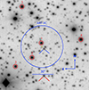 |
Fig. 1. Optical field of SRGA J213151.5+491400; source labeled by blue bars using Gaia19fld position (also, the eROSITA position) obtained with RTT150 using 1200 s exposure with a clear filter. Red bars show the comparison star used for CCD photometry. Red circles denote the standard reference stars in the field. |
The Gaia alert source, Gaia19fld, has coordinates α = 21h 31m 50 80 and δ = +49° 14′ 01
 68 and it is not included in any current X-ray catalog. The detection history of Gaia19fld is given in Table 1. The earliest Gaia brightness of the new source is 20.91 ± 0.15 mag in the G band that reveals a low state. After the alert with a flaring rise to a maximum, it remains at 17.94 ± 0.21 mag in the high state for about eight months and then starts declining. Our optical observations with the Turkish telescopes are made during this period when the source was bright (see Fig. 2). The Gaia DR3 source ID number is 1978752971571052672. There is no calculated parallax; thus, no distance estimate is possible.
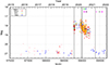 |
Fig. 2. Archival photometry of SRGA J213151.5+491400 in 2015−2022. The observations are (1) Gaia (blue); (2) ATLAS c (light pink); (3) ZTF g (red), r (light green) and i (yellow). The photometric and spectroscopic observations obtained from TUG (Türkiye) are represented with pink and green squares, respectively, while those obtained from SAO (Russia) are represented with black and blue squares. The vertical solid lines at MJD 58789, MJD 59003, and MJD 59378 indicate the dates of the Gaia alert, ART-XC detection and NICER start time, respectively. |
Observational timeline of the SRGA J213151.5+491400 X-ray source.
Figure 2 shows the long-term light curve of the new source covering the period from 2015−2022 constructed using the existing Gaia data together with the light curves from archival optical photometric surveys. We were able to retrieve the observational data from Zwicky Transient Facility (ZTF1g, r and i filters) (Masci et al. 2019) between 2018 August and 2021 January and Asteroid Terrestrial-impact Last Alert System (ATLAS2o and c filters) (Shappee et al. 2014; Jayasinghe et al. 2019) between 2015 July and 2021 November. For ATLAS, we removed poorer quality data where the uncertainty in the observed magnitude was > 2.5 mag. The o-band data of ATLAS are more scattered than the c-band and other survey data with high levels of uncertainty in the magnitudes; thus, we did not use it for the plot. The total long-term light curve indicates a low accretion state (∼21 mag) that was detected around 4−4.5 yr with ATLAS and Gaia and switched to a high state (< 18 − 19 mag) that lasted slightly over a year. In addition to Gaia and ATLAS observations, ZTF data support the notion that the system was in a higher state between November 2019 and January 2021 of ∼12 months. We note that Szkody et al. (2021) also presented ZTF data covering partly the year 2020 for SRGA J213151.5+491400 with an optical spectrum obtained using the Keck Telescope suggesting the source is a MCV candidate.
In addition to RTT150 photometry, optical photometric observations of the optical counterpart are conducted with other Turkish and Russian telescopes (1-m T100 at TUG and 1-m Zeiss-1000 at SAO RAS) and available smaller telescopes ADYU60 (60 cm) in the Adıyaman University Observatory. A log of all photometric observations from Türkiye and Russia is given in Table 2. Following the identification of the optical candidate from RTT150 photometry and MOS spectroscopy as described in the previous paragraphs, more spectral observations were performed in the standard mode with long slit aperture using RTT150 at TUG followed by spectroscopic observation using BTA at SAO RAS. A detailed list of spectroscopic observations is displayed in Table 3.
Log of photometric observations of SRGA J213151.5+491400.
Spectroscopic observations of SRGA J213151.5+491400 obtained at TUG, Türkiye and SAO, Russia.
3. Analysis and results
3.1. Optical photometry and power spectral analysis using ground-based facilities during the high state in 2020
We performed photometric observations of SRGA J213151.5+491400 between July and October 2020 (during its high state) with three different telescopes at Turkish sites as follows: Ritchey-Chretien type 1.5-m (TUG RTT150) and 1-m (TUG T100) telescopes at TUG equipped with Andor iKon-L 936 BEX2-DD-9ZQ and SI1100 CCD cameras, and a 0.6-m telescope at the Adiyaman University Application and Research Center (ADYU60) equipped with 1k × 1k Andor iKon-M 934 CCD with a pixel scale of 13 μm × 13 μm. Details including telescopes, exposure times, and filters are listed in Table 2.
Standard CCD reductions were performed on the data obtained from the 2020 observations. Since the dark counts were negligible for the CCDs used, only bias subtraction and flat-field corrections were applied. To extract the instrumental magnitude of the sources in the field, we used aperture photometry through a developed script using Python and Sextractor. We selected a comparison star with similar brightness to the new optical counterpart, Gaia19fld, in the field of view. The comparison star is shown in Fig. 1 with red bars. The Gaia source ID is 1978752975879142528 (DR3) with α = 21h 31m 50 82 and δ = +49° 13′ 23
 26 (g = 17.64). We chose a small aperture of ∼1.2 × FWHM since there is another source very close to Gaia19fld. Because our source is quite faint, relatively high signal-to-noise (S/N) values could not be obtained. For each night, a light curve was constructed using instrumental magnitude differences between the comparison and our optical counterpart. We subtracted the nightly mean differential magnitudes and converted times to HJD using Astropy timing analysis package3. Example light curves that have an adequate number of data points covering a ≥2 h time span are given in Fig. 3.
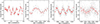 |
Fig. 3. Sample of SRGA J213151.5+491400 light curves obtained at TUG covering ≥2 h duration (with clear filter). Observation dates and telescopes from left to right are 2020 July 28 (RTT150), 2020 August 2 (RTT150), 2020 August 3 (RTT150), and 2020 October 16 (T100). Black circles are unbinned and red circles represent data binned at 7.2 min. |
The resulting light curves created from (differential) aperture photometry are used for power spectral analysis. To obtain the periodicity on individual nights, power density spectra (PDS) were constructed using a Lomb-Scargle algorithm (Lomb 1976; Scargle 1982; van der Plas 2018) provided by Astropy (Astropy Collaboration 2013, 2018). The PDS for individual nights show significant single peaks above 3σ significance for a periodicity between 82 and 93 min.
Furthermore, we performed power spectral analysis using the entire photometric light curve of the RTT150 and ADYU60 data obtained with the clear filter using the TSA (time series analysis) context within MIDAS software package version 17FEBpl1.24 and the Lomb-Scargle algorithm. In order to correct for the effects of windowing and sampling functions on power spectra, synthetic constant light curves are created and a few prominent frequency peaks that appear in these light curves are pre-whitened from the data in the analysis. Before calculating the total PDS, the individual or consecutive nights are normalized by subtraction of the mean magnitude. Moreover, when necessary, the red noise in the lower frequencies is removed by detrending the data. The top panel of Fig. 4 shows the final PDS constructed from the total photometric data using 1260 frames (for 2020 data). There is only one very prominent peak well above 3σ significance (see Scargle 1982) at 16.74770(33) c d−1 corresponding to 1.43304(2) h or 85.982 min as marked on the figure and the other peaks around the period are 1d–2d aliases. The error on the detected frequency is the half-width of the power spectral line at 99.99% enclosed power. This is calculated using the width/tsa task within the TSA context of MIDAS. The bottom panel of the same figure shows the folded mean optical light curve obtained using our time series in 2020 with the clear filter. The semi-amplitude of variations is around 0.3 mag and decreases to 0.1 mag once pre-whitening and detrending is applied. Using the same data set, we derived Ephemerides for the minimum times of this period utilizing a securely recovered modulation dip via fitting a sine curve as
 (1)
(1)
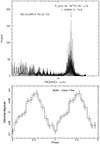 |
Fig. 4. Power spectrum and mean light curve in 2020. Top panel is the power spectrum of SRGA J213151.5+491400 derived from the entire ground-based photometric light curve in 2020 July–October (high state). The detected period is labeled on the figure. The bottom panel shows the mean light curve derived from the same data set in 2020 during the high state. The phases on the x-axis are with respect to the Tmin of the Ephemerides. |
The detected period is a typical orbital period of a CV below the period gap (the gap is at 2−3 h). On the other hand, since we did not find any other optical periodicity, we have to rely on the spectroscopic and X-ray data analysis for further classification of the CV candidate. As far as the photometry is concerned, this may be an MCV that is most likely a polar-type one since we did not find a separate spin period. It may also be a nonmagnetic CV below the period gap; however, the significant high and low state transitions are atypical of this class and more typical of polar-type MCVs.
3.2. Follow-up photometry using TUG and SAO during low state in 2021
We only performed occasional follow-up photometric observations of SRGA J213151.5+491400 in 2021 with SDSS filters since the source was very dim for time-series analysis with RTT150. Table 2 shows the log of observations in 2021 during the low state. PSF photometry is performed for the analysis. Figure 5 displays the g-band (SDSS) photometry and the mean photometric light curve (in black) of the December 2021 RTT150 data phase-locked to our derived photometric Ephemerides. The pulse profile resembles the profile in the high state, but with about a 50% decrease in semi-amplitude at ∼0.15 mag. The accumulated phase error for December 2021 data is about 0.16 and the photometric peak is at 0.2−0.3 phase (we note that this is not obtained with clear filter). Additional photometric observations were obtained at the 1 m Zeiss-1000 Telescope of SAO RAS (see Table 2). Observations were carried out both in high (2020 Oct.) and low (2021 Oct.) brightness states of SRGA J213151.5+491400. The obtained data were processed in a standard way using the IRAF5 package tools. PSF photometry was carried out. We have overplotted the mean light curve obtained from Zeiss-1000 in 2021 October (low state) using a clear filter over the mean light curve obtained of 2021 December in Fig. 5. The photometric pulse peaks at about the 0.4 phase for 2021 October, which is consistent with the peak phase in the high state within the accumulated phase error of 0.13. The slight changes in the pulse and the phase of the peak may occur as a result of the error in the period. On the other hand, the changes of accretion geometry (in high and low states) and the changes in hot spot morphology, together with usage of different filters that may reflect real color variations, can result in such phase shifts at maximum pulse phase.
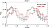 |
Fig. 5. Mean light curve of SRGA J213151.5+491400 obtained with RTT150 in 2021 December using the g-band filter (SDSS) during the low state (in black). Overplotted is the mean light curve of the source obtained with Zeiss-1000 on 2021 October 9 using a clear filter (in red). |
3.3. Optical spectroscopy using ground-based facilities during the high state in 2020
3.3.1. Long-slit spectroscopy with RTT150 at TUG
Spectroscopic data, taken from an approximately five-week period, correspond to the high state of SRGA J213151.5+491400 starting about two months after ART-XC discovery. A log of RTT150 spectroscopic observations are given in Table 3. For convenience, the times of the observations are labeled in Fig. 2 over the Gaia light curve. Long-slit (LS) spectroscopy was performed with three different grisms; No. 7 (4220−6650 Å), No. 8 (6190−8190 Å), and the broad-band No. 15 (3650−8740 Å). The slit aperture is 1 78. The resolution capacities of the grisms are: (1) No. 15 (λ/Δλ) = 749, (2) No. 7 (λ/Δλ) = 1331, and (3) No. 8 (λ/Δλ) = 2189. The exposure times for LS spectroscopy are 900 s and 1200 s for grisms No. 15 and Nos. 7 and 8, respectively. Spectrophotometric standard stars from the Oke (1974) and Stone (1977) catalogs were observed each night. Biases, halogen lamp flats, and Fe-Ar calibration lamp exposures were obtained for each observation set. Preliminary reduction steps were completed using task ccdproc within IRAF. The reductions and analysis of spectra were made using the Long-slit context of IRAF software.
Figure 6 shows the reduced, calibrated and fluxed spectra (for convenience two different grism spectra are displayed). Some of the identified lines are labeled on the figure. The LS spectrum obtained in July 2020 with grism No. 15 was used for line identification since it has the widest wavelength band with a modest spectral resolution. We list the brightest lines (with S/N > 3.0) and relative fluxes (absorbed) in Table 4. Line identification and flux determination were performed using the splot task and Gaussian fitting within the IRAF software. We find that the spectrum of SRGA J213151.5+491400 increases toward the blue continuum with strong hydrogen and helium emission lines revealing single-peaked and narrow structures. Balmer lines are the strongest. We find that the He II (λ4686) to Hβ ratio is 0.74 (see Table 4). This indicates existence of highly ionized medium via irradiation and reprocessing. Such strongly ionized helium lines are typical of MCVs with a criterion of He II/Hβ ≥ 0.4 (higher for polars) for classification (Silber 1992), which stresses that our source belongs to this class of variables. None of our spectra in the high state showed obvious cyclotron humps; however, further spectral modeling with WD, secondary star, and disk emission models to investigate the existence of cyclotron excess may improve this.
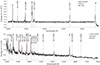 |
Fig. 6. Two long-slit spectra of SRGA J213151.5+491400 obtained during the high state with grisms Nos. 7 and 15 in the top and bottom panels, respectively. Dates of observations are labeled on the panels. Some emission lines such as Balmer lines and low ionization lines such as He I and Fe II are marked in red on the spectra. |
Emission line fluxes (absorbed) from RTT150 in 2020 July.
3.3.2. Phase-resolved MOS spectroscopy with RTT150 at TUG
We obtained 19 consecutive optical spectra each 600 s using MOS spectroscopy (see Sect. 2 for details). In contrast to the masks with pinhole apertures used to identify the source, the short slits (SS) were used in this mask with non-overlapping dispersion. In addition to the SRGA J213151.5+491400, SS were also used at the positions of secondary standards for differential spectrophotometric calibration and control of the position of the source on the slit for more correct dispersion calibration. The total duration of the MOS-spectral observations was about 3.5 h, covering about three orbital/spin periods.
The MOS spectra are analyzed in the same manner with the LS spectra using the IRAF software. A reduced and flux-calibrated set of spectra are calculated without sky subtraction to yield good S/N around prominent lines and calculate the variations of line centroids while following sky lines for calibration purposes. We selected three well-recovered Balmer lines, Hγ, Hβ, and Hα, and derived the line centroids via fitting Lorentzian profiles along with a constant continuum value around the line of interest. Figure 7 shows the calibrated and normalized variation of all three line centroids where the mean value of the detected line center is subtracted. We do not find any phase-shifts between different Balmer line variations (see ϕ0 in Eq. (2)), which help to construct the figure, but there are different amplitude variations for each line center that mimic y error. We followed a sky line of O I at 5577 Å (green line) for calibration purposes of line centroids, which showed a variation of < |0.3| Å throughout the 3.5 h, considerably less than the centroid variations of Balmer lines. Next, we analyzed the data in Fig. 7 using a Lomb-Scargle algorithm that yielded a spectroscopic period of 0.0609(20) d (detected well over 3σ significance). The error corresponds to the half-width of the power spectral line at 99.89% enclosed power. We checked the individual line variations and they all show a similar periodicity. This period is longer than the photometric period we calculated by about 2%. However, the error range of the spectroscopic period overlaps with the photometric period, making this a regular polar-type MCV system.
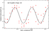 |
Fig. 7. Variations of relative change in wavelengths of Hγ, Hβ, and Hα lines versus time covering three periods. |
3.3.3. Long-slit spectroscopy with BTA at SAO, RAS, and the radial velocity curve
Since SRGA J213151.5+491400 is a dim source for RTT150, particularly for time-resolved studies, additional spectral observations of SRGA J213151.5+491400 were carried out at the 6 m telescope BTA of the SAO of the Russian Academy of Sciences. The telescope is equipped with the SCORPIO-1 focal reducer in long-slit spectroscopy mode (Afanasiev & Moiseev 2005). The observations were performed on the nights of 2020 September 25 and 26 in good astroclimatic conditions with seeing of 1 2−1
2−1 5. These dates are about four months after the ART-XC discovery during the onset of decline from the high state. On the first night, the grism VPHG1200G was used and provides an effective spectral resolution of ∼2.6 Å pix−1 with 1
 2 slit width covering the 3900−5800 Å spectral region 20 spectra were obtained in two hours. On the second night, three spectra were obtained using VPHG550G grism with corresponding effective spectral resolution ∼6 Å pix−1 in the 3500−7500 Å spectral region. All spectra were obtained with an exposure of 300 s. The data reduction was carried out using the IRAF package in a standard fashion. Cosmic-ray events were subtracted using the LaCosmic algorithm based on the Laplacian edge detection technique (van Dokkum 2001). Pixel-to-pixel variations were removed by flat-field exposures. The He-Ne-Ar arc frames were used for wavelength calibration and geometrical corrections. The spectra were extracted using an optimal extraction technique (Horne 1986) with the subtraction of the background light. The flux calibration was performed using the spectra of standard star G191B2B. A signal-to-noise ratio of S/N = 7 − 8 was acquired in the 4300−5000 Å range with the VPHG1200G grism during the entire observation excluding the last three spectra that were obtained under light cloud cover.
The average BTA spectra obtained with VPHG550G and VPHG1200G grisms are shown in Figs. 8a and b, respectively. We note that before averaging, the spectra were shifted to the same radial velocity RV ≈ 0 km s−1. The presented spectra are typical for magnetic cataclysmic variables. The main features of the RTT150 LS spectra are detected in the BTA LS spectra as well. There is a strong He II ∼ λ4686 line with strength  of the Hβ line, which is typical for MCVs. The VPHG550G spectra do not show any “humps”, which could be interpreted as cyclotron harmonics. We note that the BTA LS spectra may not be very similar in flux (line or continuum) to the RTT150 LS spectra of TUG since the source brightness had started to diminish in September 2020 and there are about two months between RTT150 and BTA spectra taken at the end of 2020 September.
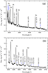 |
Fig. 8. Average BTA spectra obtained by VPHG550G (a) and VPHG1200G grisms (b). |
Dynamical spectra of Hβ and He IIλ4686 lines are shown in Fig. 9. The figure shows the evolution of the spectral profiles during the observations. The photometric phases of spectral observations are calculated using the Ephemerides (Eq. (1)) and plotted along the Y-axis. It is seen that the lines exhibit variability due to radial velocity and intensity changes. There are noticeable differences in the behavior of the He IIλ 4686 line in comparison with the Hβ line. All lines are single-peaked at all observed phases, indicating the absence of an optically thin accretion disk, for which double-peaked line profiles would be expected. This agrees well with our assumption of the polar-type MCV nature of SRGA J213151.5+491400 and is consistent with the results of RTT150 TFOSC spectra.
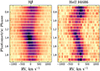 |
Fig. 9. Dynamical spectra of Hβ and He IIλ4686 lines. |
The radial velocities of emission lines were calculated by the cross-correlation technique of Tonry & Davis (1979) applied in the 4000−5500 Å region of the VPHG1200G spectra. The determination of radial velocities was performed in two steps. At the first step, the radial velocities were determined using the first spectrum as a template. At the second step, the derived velocities were removed from each spectrum and the spectra with new wavelength scales were averaged. Then, we improved radial velocities using the average spectrum as a template. The resulting radial velocity curve is shown in Fig. 10.
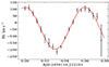 |
Fig. 10. Observed radial velocity curve fit by the sine function using the detected spectral period. |
The spectroscopic period was determined by the least-square fitting of the observed RV-curve by the function
 (2)
(2)
where P is the desired period, t is the epoch of mid-exposure, K is the radial velocity semi-amplitude, and φ0 is phase shift. The best-fit orbital period is P = 85.6 ± 2.2 min ( ). Uncertainty of the orbital period has been found with the Monte Carlo error back-propagation technique assuming normal distribution of radial velocity errors (1σ deviation was used as the error of the period). The best-fit sine curve is plotted on the radial velocity curve in Fig. 10. The semi-amplitude of the optimal sine curve is K = 155 ± 6 km s−1. The top and bottom panels of Fig. 11 compares the behavior of the radial velocities and brightness of SRGA J213151.5+491400 using the photometric phases calculated from the Ephemerides (Eq. (1)). The mean light curve in the bottom panel is the same in Fig. 4; however, it is unbinned in the phase. The radial velocity curve is shifted relatively to the sinusoidal light curve by Δφ ≈ 0.25.
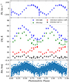 |
Fig. 11. Radial velocity curve (upper panel), equivalent width curves of four emission lines (middle panel), and photometric light curve (lower panel) of SRGA J213151.5+491400. All curves were phased according to Ephemerides (Eq. (1)). |
The behavior of the equivalent widths of several strong lines over the orbital period is shown in the Fig. 11 during the high state. The EW errors were estimated using a Monte Carlo technique. The modulation of EWs with the orbital period is clear. All analyzed lines exhibit a single-peaked EW curve, except perhaps the He II ∼ λ4686 line, which indicates a double-peaked structure. It should be noted that the EW curve of the He II ∼ λ4686 line differs from that of the hydrogen lines. Thus, the maximum of the EW of the hydrogen lines is near phase φ ≈ 0.35, while the curve of the EW of the ionized helium line reaches a maximum near φ ≈ 0.85. It can be seen that the most dramatic EW variation ([EWmax − EWmin]/EWmin) is with the He II ∼ λ4686 line and is of about 60%, while the Hβ and Hγ lines have EW amplitudes of ∼45% and ∼35%, respectively. Figure 11 does not show any explicit correlation or anticorrelation between the EW of lines and the brightness of the system in photometric bands (i.e., in the continuum). Thus, the flux in the lines changes during the orbital period, which indicates a high optical thickness in the line-emitting regions and/or obscuration by the donor (the latter requires high inclination > 40°).
3.4. X-ray spectral and temporal data analysis
3.4.1. NICER observation in the low state
We used HEASOFT6 (version 6.29) to perform the NICER analysis and utilized XSELECT7 (version v2.4-e) to obtain light curves and a spectrum using the cleaned events created via the nicerl2 data reduction tool as described in Sect. 2. A background spectrum for our observation was created with the nibackgen3c50 tool and response and ancillary files were generated using the tasks nicerrmf and nicerarf, respectively, to perform spectral analysis. Further analyses were conducted within the HEASOFT environment utilizing XSPEC8 for spectral and XRONOS9 for temporal analyses. We underline here that the NICER observation was obtained in the low state after the source diminished by about 3 magnitudes in the optical. During the construction and writing of the manuscript, another updated version of NICERDAS was released in December 2022, NICER version-2022-12-16-V010a, with the calibration database xti20221001 including data product tasks nicerl3-spect and nicerl3-lc for spectral and light-curve extractions. We used the new software to check for the consistency of results between different software versions and background checks. The results below use the NICERDAS v.2020-04-23-V007a (and caldb xti20210707) unless an improvement was found with the new version, NICERDAS v.2022-12-16-V010a.
Below, we present the light-curve analysis performed using NICERDAS v.10a and nicerl3-lc10 task. After creating a total light curve in the NICER range, a standard power spectral analysis was conducted, which did not reveal any other periodicity. We folded the total X-ray light curve using the optical photometric Ephemerides we determined in this work (the accumulated phase error at the time of the NICER observation is ∼0.1). The resulting folded mean X-ray light curve from 0.25−7.5 keV is displayed in the top panel of Fig. 12. This plot shows variation of the X-ray flux at the orbital period (which for a polar-type MCV coincides with the WD spin period).
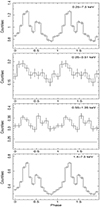 |
Fig. 12. NICER pulse profile of WD spin (orbital) period in three different energy bands (NICER 2021 June 13) calculated using light curves created with nicerl3-lc task. The bands are labeled on the panels. The light curves are folded over the optical photometric Ephemerides in Eq. (1). The background count rate calculated from the light curves for each band is denoted with the solid horizontal line. |
We also computed pulse profiles in three energy bands: 0.25−0.5 keV, 0.55−1.35 keV, and 1.4−7.5 keV. They are shown in the three panels below the top panel in Fig. 12. The figure shows a lack of strong modulation at the low energies below 1.4 keV and more significant modulation in the 1.4−7.5 keV band, where the pulse profile has a double-peak structure. This indicates two-pole accretion in the system. An approximate estimate11 of a pulsed fraction, (Fmax − Fmin)/(Fmin + Fmax), in this energy range is ∼(30−40)%. The estimates for the other ranges are low: ∼(10−15)% for 0.25−0.5 keV and ∼10% for the 0.55−1.35 keV range. The pulse profiles (mostly sinusoidal) in the optical and X-ray bands do not show evidence of an eclipse. For example, a two-pole accreting polar detected in the X-rays, V496 UMa, shows similar double-peaked pulse profiles to ours (Kennedy et al. 2022; Ok & Schwope 2022). We also clarified that the 92.6 min orbital period of the spacecraft does not affect the modulation detected at the WD spin period or affect the light-curve modulations in different energy bands.
After creating the spectrum (using XSELECT) and calculating a background spectrum via the tool nibackgen3c50, these were incorporated in XSPEC along with the proper ancillary and response files for spectral modeling and statistical analysis. The background estimator, nibackgen3c50, models both the non-X-ray and the X-ray sky background contributions. There is a clear soft excess in the NICER spectrum (Fig. 13), and we used a TBABS × (BBODY+CEVMKL) composite model to derive the spectral parameters that describe the source emission in the 0.25−10.0 keV range. BBODY is a blackbody model of emission, and CEVMKL (Singh et al. 1996) is a model of multi-temperature plasma emission in collisional equilibrium with variable plasma abundances built from the MEKAL code (Mewe et al. 1986). The fits are performed using interpolation on pre-calculated MEKAL tables with abundances fixed at solar values. However, fits and error ranges are checked against the same code running using the ATOMDB12 database. The top panel of Fig. 13 displays the fitted NICER spectrum using the 3C50 background model. This is in accordance with the expectations of emission from the stand-off shock near the WD surface in the accretion column. We note here that there is no disk, and the accreting material is carried along the magnetic field lines via an accretion funnel.
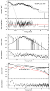 |
Fig. 13. NICER spectrum and spectral fits. Top panel shows X-ray spectrum of SRGA J213151.5+491400 obtained with NICER between 0.25−10.0 keV (using 3C50 background model). The spectrum is fit with TBABS × (BBODY+CEVMKL) labeled with dotted lines and the residuals in the lower part are in standard deviations for all panels. The middle panel shows a spectrum derived using a very stringent undershoot parameter range of 0−50 to clear the dominant soft X-ray noise peak below 0.5 keV, which is fit with only a CEVMKL model using the 3C50 background model. The bottom panel shows the same spectrum created using the SCORPEON background model with different variable background contributions, fit without the blackbody component (see text for details). |
The two-component fits to the NICER spectrum (in the top panel of Fig. 13) yield an NH of (0.5−0.95) × 1021 cm−2 using abundances set to “wilm” (Wilms et al. 2000) (90% confidence level range for a single parameter). The Galactic absorption in the direction of the source is (6.46−6.74) × 1021 cm−2 and is calculated via the nhtot13 tool devised using the GRB data of Swift Observatory (Willingale et al. 2013). The NH value from the spectral fit is about 5−10 times lower than the interstellar absorption in the direction of the source. This suggests that the source is located in front of the main absorbing material in this direction (e.g., source is closer by) and that the intrinsic absorption is also low, with perhaps some partial covering and ionized absorption in effect.
The other spectral parameters of our modeling yield parameter ranges using the CEVMKL model, with the power spectral index of the temperature distribution α = 1 being (1) kTmax = 3.0 − 6.0 keV, (2) N = (4.0−6.1) × 10−4, (3) kTBB = 0.015−0.018 keV, and (4) NBB = (0.3−2.4) × 10−2. When α is not fixed (for CEVMKL), these spectral parameters change to (1) kTmax = 7.4−13.5 keV, (2) N = 1.7−4.7 × 10⁻⁴, (3) kTBB = 0.015−0.019 keV, and (4) NBB = (0.6−4.5) × 10−2, with an α in the 0.5−0.7 range. All error ranges correspond to a 90% confidence level for a single parameter. NBB is the normalization of the BBODY, and N is the normalization of the CEVMKL model, where N = (10−14/4πD2) × EM and EM (emission measure) = ∫nenH dV (integration is over the emitting volume V). We note that the spectral data products and these parameter ranges are consistent for different NICERDAS software versions (v.7 and v.10a) as the fits were checked using both.
The absorbed flux derived from the fits is about 5.0 × 10⁻¹³ erg s−1 cm−2 in the 0.2−10.0 keV band. The soft X-ray and the hot plasma components have absorbed fluxes of 1.0 × 10⁻¹³ erg s−1 cm−2 and 4.0 × 10⁻¹³ erg s−1 cm−2, respectively, in the 0.2−10.0 keV band. The unabsorbed fluxes in the same energy band and at the 90% confidence level are (6.0 × 10⁻¹³–2.0 × 10⁻¹²) erg s−1 cm−2 (for the soft component) and (1.7 × 10⁻¹³–5.8 × 10⁻¹³) erg s−1 cm−2 (for the hot plasma), respectively.
The α parameter of 1.0 signifies a standard cooling flow plasma in collisional equilibrium. The change of this value from 1.0 indicates that the flow deviates from a cooling flow and that the flow does not cool effectively. The temperature range derived from the variable α value is higher with plasma temperatures of 7.4−13.5 keV, as expected. We find that the fit with no fixed α parameter (χ2 = 279.9 d.o.f. = 249) is better than the fit with α = 1.0 (χ2 = 290.0 d.o.f. = 250) at a 99.99% confidence level, at over 3σ significance (using an FTEST in XSPEC). If ATOMDB (database) is used to calculate the plasma model, the discrepancy in total χ2 yields a 90% confidence level difference between the fits.
The NICER spectrum of SRGA J213151.5+491400 shows a prominent soft component in its spectrum below ∼0.5 keV (0.25−0.5 keV). To our knowledge, this the first time such a component is detected in the low state of a polar. Below, we discuss and eliminate several contaminating factors that may affect the reliability of its detection.
The NICER spectra are contaminated by the low-energy noise peak below 0.25 keV resulting from undershoots14 (strongest background component). We checked how much this may affect our detected soft X-ray component. To this end, we used a highly conservative constraint on the undershoot count range (∼0−50) in data screening that minimizes the low-energy noise contributions to almost zero. This method yielded a (5−7)σ excess in the residuals from 0.25−0.5 keV, while the neural H column density parameter was left free (see middle panel of Fig. 13). The NICER calibration team (NICER SOC) cordially checked any anomaly in the background and noise characteristics of our data and the observation confirming the soft X-ray component of the source.
In order to check the possible contribution of soft X-ray background to the soft component found in the NICER spectrum of SRGA J213151.5+491400, we also used the SCORPEON background model (using NICERDAS v.2022-12-16-V010a and nicerl3-spect task), where one can obtain composite (modelable) background components (produced via a script) along with the data products to use in the fitting process. Our fits revealed that when utilizing the SCORPEON model, the spectral parameter ranges for our source are consistent with the results using a varying α parameter and a slightly higher temperature than in the above paragraph (an α of 1 is acceptable within the parameter space). Firstly, we checked the soft X-ray contribution from the local hot bubble (LHB) and varied the emission measure parameter of the LHB out to 50−100% of the best-fit value. The best-fit value of 1.6 × 10⁻³ cm−3 pc is consistent with the sky maps presented in Liu et al. (2017) around the coordinates of our source (solar charge exchange contribution subtracted), and the enhancement we used is larger than what is permitted by values on these maps. We found that LHB cannot account for the soft excess below 0.5 keV yielding a (5−6)σ variation in the fit residuals (see bottom panel of Fig. 13; the red line is for total X-ray sky background). We also varied the SWCX (solar wind charge exchange) sky-background parameters (the charge exchange line emission by the heliosphere) to account for the expected lines (e.g., O Kα, O VII, O VIII, Ne IX – 0.5−1.0 keV) in the background emission, which also reduced residual fluctuations (see bottom panel of Fig. 13, the red line between particularly 0.5−0.9 keV). We derived best-fit line fluxes as 2.2 (O Kα), 5.4 (O VII), 6.4 (O VIII), and 2.7 (Ne IX) in LU (line units, photons s−1 cm−2 sr−1). During these fits, the LHB background was fixed at a value 50% larger than the best fit. The SWCX line fluxes found from the fits are large and enhanced compared to the average maximum permitted values of 4.6 LU for O VII and 2.1 LU for O VIII (see Koutroumpa et al. 2007; our values are 1.2 times larger for O VII and 3 times larger for O VIII). We note that the maps in Liu et al. (2017) and surveys therein including the ROSAT RASS (all sky survey) indicate that the field around our source is empty with no sign of excessive diffuse emission in the vicinity. Therefore, the bottom panel of Fig. 13 shows that even when highly elevated values of LHB and SWCX sky backgrounds are assumed, there is a soft X-ray excess at (5−6)σ as observed in the residuals that can not be modeled by background effects.
We note here that the field of view of NICER is 5′. We have checked the X-ray position of our source for unrelated sources using all available archival X-ray data, X-ray surveys, and X-ray catalogs. We found no other X-ray source in the field of view of NICER (this is why it was proposed). This is larger than the error box we used for optical identification. We stress that in the 1′ search diameter, where we found 30 optical counterpart candidates down to 20−21 mag (and derived their spectra), we had no source that was blue enough and showed as an interacting system that would be emitting X-rays other than Gaia19fld. Particularly, there was no indication of a strong UV candidate that would yield a detection of ∼15 eV blackbody emission as in NICER, other than Gaia19fld. Moreover, neither eROSITA (half point diameter (HPD) ∼ 15″) nor ART-XC (HPD ∼ 30″) imaging surveys detected any other X-ray source in the vicinity of the new source within the 5′ field of view (FOV) of NICER during the four scan periods in 2020 and 2021. We checked all Gaia alerts, and there were no other transients in the 5′ vicinity of Gaia19fld detected after its increase in the years 2020 and 2021.
3.4.2. eROSITA observations in the high and low states
Our source, SRGA J213151.5+491400, was detected in each of the four all-sky surveys performed by the SRG observatory in 2020−2021. eROSITA observations took place during the following time intervals: 2020 June 2−4, 2020 December 6−8, 2021 June 6−8, and 2021 December 10−12. eROSITA provides good quality spectral information in the 2020 high state of the source not covered by NICER observations.
The eROSITA raw data were processed by the calibration pipeline developed in the eROSITA X-ray catalog science working group at the Space Research Institute (IKI, Moscow, Russia) using the calibration tasks of the eROSITA Science Analysis Software System (eSASS) developed at the Max-Planck Institute for Extraterrestrial Physics (Garching, Germany) and the data analysis software developed in the RU eROSITA consortium at IKI. We excluded telescope modules 5 and 7, affected by the optical light leakage, from the analysis. The spectra and light curves of the source were extracted using the circular aperture with radius of 60″ centered at the source position. An annulus region with the inner and outer radii of 120″ and 300″ was used for the background estimations. The response files were created using the eSASS tasks. Spectral and temporal analysis were performed using XSPEC and XRONOS packages within the same HEASOFT environment as in Sect. 3.4.1. Here, we report on the spectral analysis results.
For the high state, we simultaneously fit the two spectra collected during the first and second all-sky surveys on 2−3 June and 6−8 December, 2020. All model parameters were linked for the two spectra, except for normalizations. A single component XSPEC model TBABS × CEVMKL provided adequate description of the observed spectra in the high state given the spectral statistics. Similarly to the approach used in the NICER data analysis, we performed two types of fits fixing the α parameter of CEVMKL model to 1 or making it a free parameter of the fit. We used the CEVMKL model with the ATOMDB database. For α = 1, we obtained the following spectral parameter values: (1) kTmax = 76.8 keV and (2) N = (8.0
 ) × 10−3 and N = (5.4
 ) × 10−3 for the first and second surveys, respectively. N is the normalization of the CEVMKL model (see Sect. 3.4.1 for the description). The NH parameter was
  cm−2, which is consistent with the NICER value. Similarly to NICER spectral fits, this value is almost an order of magnitude smaller than the Galactic value. The C-statistical value of the fit is 109.6 for 110 degrees of freedom (using Survey 1 and 2 spectra). The plasma temperature in the accretion column is unconstrained with the lower limit of kTmax > 21 keV at the 95% confidence level (using ATOMDB). The lower limit changes to kTmax > 17 keV when using an interpolation on pre-calculated MEKAL tables (see Sect. 3.4.1). For α thawed, we obtained only an insignificant reduction of the C-Statistics (= 102.7 for 109 degrees of freedom) and obtained a best-fit value of α = 1.3 with a lower limit of α > 0.7 (95% confidence level).
Given no improvement in the fit statistics, and the fact that an α of 1.0 is acceptable within the error range, a standard cooling flow model can be used for the physical interpretation of the high state. Figure 14 displays the spectra obtained in the first and second surveys along with their best-fit model (using α = 1). As one can see, in the high state there is no soft component as apparently present as that in the low state spectrum obtained with NICER (cf. Fig. 13). However, the CEVMKL continuum level is about an order of magnitude higher in the high state, and the presence of a soft component with the parameters measured by NICER is consistent with the eROSITA data. The 90% upper limit on the absorption corrected flux (0.2−10.0 keV) of a blackbody component with the temperature equal to a NICER best-fit value of 15 eV is 7.6 × 10⁻¹¹ erg s−1 cm−2 larger than the unabsorbed flux range measured by NICER in the same energy band.
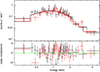 |
Fig. 14. X-ray spectra of SRGA J213151.5+491400 fit with TBABS × (CEVMKL) model. Data was obtained with SRG/eROSITA telescope in the course of two sky surveys in 2020 (high state). The lower panel shows the residuals in standard deviations. |
The two spectra obtained by eROSITA in the third and fourth sky surveys in 2021 have relatively low number of counts (about ∼25 − 30 counts each) and do not provide statistically significant spectra in the low state. These spectra are generally consistent with NICER results. The absorbed fluxes of the best-fit models measured in the four SRG/eROSITA surveys are (6.3 ± 0.8)×10−12 erg s−1 cm−2, (4.3 ± 0.6)×10−12 erg s−1 cm−2,  erg s−1 cm−2, and
  erg s−1 cm−2 in the 0.2−9.0 keV band.
4. Discussion
4.1. Doppler tomography in the high state
The behavior of emission line profiles as a function of the orbital phase is analyzed by the means of Doppler tomography technique, which is aimed at reconstructing the distribution of emission regions in the two-dimensional velocity space. Each point in this space has two polar coordinates: v and ϑ. v is the absolute value of the velocity (relative to the center of mass) projected to the line of sight, and ϑ is the angle between the velocity vector and the direction to the secondary as is seen from the center of mass (see Kotze et al. 2015, 2016 for details). In this work, Doppler tomograms were reconstructed with a doptomog code (Kotze et al. 2015), which implements a maximum entropy regularization technique. Moreover, we used the so-called flux-modulated variant of Doppler tomography, which assumes sine-like variability of emission points during the orbital period. This option is preferable for studying an optically thick medium (Steeghs 2003). The Doppler tomograms can be reconstructed in two projections: standard and inside-out. In the standard projection, the absolute value of velocity v increases from the origin of the tomogram to the periphery which is a good choice for analyzing low-velocity structures, the high-velocity structures are blurred. The inside-out projection eliminates this problem using an absolute velocity that increases from the periphery to the center of the tomogram (Kotze et al. 2015). Based on the available observations, it is impossible to construct an orbital ephemeris for SRGA J213151.5+491400. The system is not eclipsing, and the spectra do not show lines (or line components) formed on stellar components. Due to the absence of orbital ephemeris, we assumed that orbital phases φorb (where φorb = 0 is taken as the closest approach of the secondary to the observer) are related with photometric phases φ as φorb = φ + 0.76. Using this relation, we achieved the best agreement between the emission distribution on the Doppler tomogram and the theoretical accretion stream velocities. The regularization parameter used in the maximum entropy method was selected by an L-curve criterion (see, e.g., Hansen & O’Leary 1993).
The Doppler tomograms were reconstructed using the spectral data obtained with the VPHG1200G grism on BTA/SCORPIO. The tomograms in standard projection for the Hβ, Hγ, and He IIλ4686 lines are presented in the upper panel of Fig. 15. They are one-spotted, and the position of spots is clearly different for He IIλ4686 and Balmer lines. Also, there is slight elongation of emission spots, which may indicate the direction of accretion flow. Any ring-like structure that could correspond to an accretion disk does not appear in tomograms, which confirms the polar nature of SRGA J213151.5+491400. The Doppler tomograms using inside-out projection are presented in the lower panel of Fig. 15. The tomograms show the high-velocity (v > 500 km s−1) component of the accretion stream directed to the center. The possible separation of the stream into two components is noticeable in the tomogram for He IIλ4686 at 500 ≲ v ≲ 750 km s−1 and 135 ≲ ϑ ≲ 200°. This separation can be caused by the transitions of the accreted gas from the ballistic to the magnetic trajectory. For a demonstration of this effect, we superimposed on the tomogram the theoretical velocities of particles starting from the Lagrangian point L1. At first, the particles move along a ballistic trajectory calculated by solving the restricted three-body problem. Then they abruptly switch to a magnetic trajectory described by a dipole model. To perform these calculations, we set the secondary mass M2 = 0.1 M⊙ satisfying the empirical relation  of Warner (1995). The mass of the white dwarf is taken to be M1 = 0.83 M⊙ as the most probable primary mass in cataclysmic variables (Zorotovic & Schreiber 2020). The inclination is fixed at i = 50° by fitting the theoretical ballistic trajectory to the observed one on the Doppler tomogram. The magnetic trajectories are calculated for three azimuth angles (10°, 20°, 30°) which determines the position of the ballistic-to-magnetic trajectory transition region. Signs of stream separation into two components (ballistic and magnetic) in Doppler tomograms are typical for polars (Schwope et al. 1997). Other signs of stream separation into two components recovered from inside-out projections are V834 Cen (Kotze et al. 2016), BS Tri (Kolbin et al. 2022), and V884 Her (Hastings et al. 1999; Tovmassian et al. 2017).
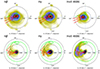 |
Fig. 15. Doppler Tomography. Upper panel: Doppler tomograms for Hβ, Hγ, and He IIλ4686 in standard projection. Lower panel: same as upper panel, but in inside-out projection. Closed dashed line and closed continuous lines are velocities of primary and secondary Roche lobes, respectively. The green line is the trace of ballistic stream in velocity space. The red lines are velocities of a gas stream at three dipole lines. |
4.2. Comparison of X-ray emission in different source states
Polars (or AM Her systems), unlike nonmagnetic CVs or intermediate polar systems, do not have a disk and a reservoir of material for that purpose. As a result, when mass transfer ceases, accretion stops. In high accretion states (ṁ ≥ 1 g s−1 cm−2), the density of the accreting gas in the accretion column is high enough to maintain a collisional timescale shorter than the cooling and dynamical timescales; hence, the flow is hydrodynamic and a stand-off shock forms in the accretion column near the WD surface forming the hard X-ray component and the soft X-ray component forms via the reprocessing of the hard component (Basko & Sunyaev 1975; Lamb & Masters 1979). A widely accepted model for the soft X-ray component during the high state is the “blobby accretion”, where over-dense blobs surpass the shock and thermalize in the atmosphere (Frank et al. 1988). This scenario requires at least Lsoft/Lhard ∼ 10 in the X-ray band and at high H column densities. In our study, we do not recover the soft component in the high state, and in both states column density of H is low. Thus, blobby accretion is unlikely. In lower accretion rate states, (ṁ ≤ 1 g s−1 cm−2), it has been suggested that collisions in the shock heated gas may be inefficient, and the Coulomb collisions of charged particles in the WD photosphere may be the way kinetic energy of the accreting gas is released (Ramsay et al. 2004; Woelk & Beuermann 1993). Surveys of polars using XMM-Newton and Swift show that the soft X-ray components are absent in low states with detected hard X-ray plasma emission from the stand-off shock with temperatures ≤5 keV at luminosities ≤1 × 1030 erg s−1 (Ramsay et al. 2004; de Martino et al. 2020, and references therein). The luminosities in the low state are ∼ a factor of 100 less than the high state (Ramsay & Cropper 2004). In general, polars change accretion state to a low state with a 3−4 mag difference in their V magnitude (this change can be 1.5−4 mag if intermediate states are considered).
SRGA J213151.5+491400 changed to a low state at the beginning of 2021 from the high state in 2020 with 3 mag decrease in system brightness. NICER spectral results indicate that the neutral H column densities are low. For the hard X-ray component in the low state, we detect a somewhat higher X-ray temperature in a range of 7.4−13.5 keV when the α parameter is not fixed (i.e., 0.3−0.7) as opposed to ≤5 keV generally measured in the low state polars. However, we note that the 3.0−6.0 keV range detected with α = 1 (at lower significance) is more consistent with the range derived in earlier polar surveys that assumed α = 1 in spectral modeling. eROSITA data in the 0.2−9.0 keV range yield a factor of only ∼10−15 difference between the high and low state fluxes for the hot plasma component (unabsorbed), which is confirmed by the NICER data as well. We also found that the NICER pulse profiles indicate energy dependence where the pulsed fraction below 1.4 keV is 2−3 times less than the fraction above 1.4 keV. In the X-ray regime of polar-type CVs, occultations of the hotspot or the accretion column by the WD are expected features in the light curves producing modulations/variations (Hellier 2014; Mukai 2017). Photoelectric intrinsic absorption produces pulsed fraction that decreases with increasing energy in MCVs, mostly IPs, produced in the pre-shock accretion curtain (Osborne 1988; Hellier 2014; Mukai 2017). The type of energy dependence we derive cannot be properly explained in this context. We also do not find prominent eclipse effects in the optical or X-rays. Norton & Watson (1989) calculated modulation depths in the X-rays (see Fig. 4 in this paper) as a result of a simple cold absorber or a patchy partial covering absorber, where they found that the partial covering absorbers dilute the X-ray modulations and diminish or suppress the low energy (below 1 keV) pulsed fractions of the spin periods. This is in accordance with our findings and hints at a complex absorption scheme in our source; however, our NICER spectrum is not statistically adequate to perform modeling involving complex absorption. A decreased pulsed modulation in the lower energy band below ∼1−1.5 keV has been observed in cases such as V496 UMa (Ok & Schwope 2022), V1432 Aql (Singh & Rana 2003), 1 RXS J2133.7+5107 (Anzolin et al. 2009), IGR J19552+0044 (Bernardini et al. 2013), and YY Dra (Yazgan & Balman 2002).
We detect the first soft X-ray component of a polar system in the low state with a blackbody temperature of 15−19 eV using NICER data. This blackbody temperature is at the lower end of the blackbody temperature range of polars, 20−60 eV, determined from surveys (de Martino et al. 2020). eROSITA data in the high state are consistent with the presence of the detected soft X-ray component by NICER. We calculated a stringent, unabsorbed, soft X-ray flux range performing fits with the SCORPEON variable background model (utilizing NICERDAS v.10a), using correct model values from literature and fitting the X-ray sky background with its correct components to the NICER spectrum (see also Sect. 3.4.1). We arrived at a best-fit temperature of 16.5 eV with a 2σ error range of unabsorbed blackbody flux of (2.8−20.3) × 10−11 erg s−1 cm−2 in the 0.1−10.0 keV range (calculated using the contour plots of temperature and normalization around best-fit parameters). This energy range of soft X-ray blackbody flux underestimates the bolometric luminosity/flux by a factor of only 18.
The high state shows a dominant hot shocked-plasma component, kTmax > 21 keV (lower limit at 95% confidence level), with a low NH value of  cm−2, and this value does not change in the state transition. The new MCV may be related to a recently proposed class of hard X-ray polars characterized with high X-ray temperatures and lack of the soft component in normal or high states (e.g., Bernardini et al. 2014, 2017). These systems are detected by Swift BAT and some with INTEGRAL. Presently, 13 out of 130 known polar systems are suggested as hard X-ray polars (de Martino et al. 2020; Bernardini et al. 2019) and none has been found to show a soft X-ray component in any state as opposed to the one detected in this study using NICER.
5. Summary and conclusions
We optically identified a new polar-type magnetic cataclysmic variable discovered by SRG observatory during its all-sky survey. The source was discovered in 2020 during a prominent flare, near its peak, and we observed it transmitting to the low state in 2021. Optical and X-ray data were collected both in high and low states of the source.
We find the spin period of the WD (for standard polars, it is also the orbital period) to be 0.059710(1) d (85.982 min). We do not find any other periodicities in the optical or X-ray data. This period is one of the shortest (below the period gap) for polar-type systems. The orbital/spin pulse profile of the source is single peaked (mostly sinusoidal) in the high state, determined from the optical (TUG) data (∼0.3 mag semi-amplitude of variations). In June, 2021 (within the low state), the NICER X-ray light curves shown in Fig. 12, portray a double-peaked profile indicating a two-pole accretor. One of the maximum peaks is at the phase of ∼0.5, where the single peak in the optical exists during the high state (the accumulated phase error is ∼0.1 for NICER data). However, optical photometry in the low state of the source in 2021 with Zeiss-1000 (October) and TUG (December) showed a single-peaked pulse profile, similar to the one found in the optical band in the high state. We note that we do not have simultaneous optical and X-ray coverage. Change of accretion geometry and pole-switching from one to two-pole accretion within or across states is detected in several polar MCV systems (e.g., Schwarz et al. 2002; Beuermann et al. 2020, 2021; Ok & Schwope 2022).
We studied the spectrum of the new polar MCV during the high state in the optical (using TUG-RTT150 and SAO RAS-SCORPIO-1). Our low-resolution spectroscopy revealed prominent Balmer lines with absorbed fluxes in a range (2.2−3.8) × 10−14 erg s−1 cm−2 Å−1 and a prominent HeII line with an absorbed flux of 2.8 × 10⁻¹⁴ erg s−1 cm−2 Å−1. The continuum does not reveal cyclotron humps in the high state. We have not been able to obtain long spectroscopic observations to find a well-constrained spectroscopic period, but it agrees with the photometric period. However, the asynchronism of the WD needs to be investigated. The EWs of all the Balmer and He lines show variation over the photometric period of the WD and the detected EWs are consistent with recent results on polars (see Table 5 in Beuermann et al. 2021).
Our study of Doppler tomography using the Balmer and He lines confirmed the polar MCV nature of the system. For polars ballistic section of the accretion flow is bounded by the region around the Lagrangian point L1 and the boundary defined by Alfven radius. An increasing accretion rate and a decreasing magnetic field induction lengthen the ballistic trajectory (Bisikalo et al. 2021). Hence, our detection of the ballistic stream in the high state was to be expected for a polar system. This is also predicted to affect the morphology of the polar caps.
SRGA J213151.5+491400 was discovered in the X-rays by ART-XC in the course of the SRG all-sky survey and followed-up with NICER in the low state. eROSITA data were contemporaneous with ART-XC and provided accurate position and the spectral data of the X-ray source in the high state. One of the important findings of our study is the detection of the soft X-ray component in the NICER data. This is the first detection of a soft component in the low state of a polar. Formal blackbody fits to the NICER data give a temperature of 15−18 eV with an unabsorbed flux of (2.8−20.3) × 10−11 erg s−1 cm−2 in the 0.1−10.0 keV band.
In the low state, we find that the plasma component remains hot around 7.4−13.5 keV (consistent with 3C50 and SCORPEON background analysis), whereas in the high state the shocked plasma temperatures (in the PSR) are kTmax > 21 keV (lower limit at 95% confidence level). The low state and high state (hot plasma) unabsorbed fluxes are ∼4.0 × 10⁻¹³ erg s−1 cm−2 and ∼6.0 × 10⁻¹² erg s−1 cm−2, respectively. This translates to a decrease of about a factor of 10−15 in unabsorbed flux for the hard X-ray (shock) emission spectrum in the 0.2−10.0 keV range from the high into the low state, which is about a factor of 5−10 times smaller than expected. We find a range of low NH, 0.5 × 10²¹–0.95 × 1021 cm−2, which does not seem to change between high and low states. This value is about 5−10 times smaller than the Galactic absorption toward the source. It may suggest that the source is located in front of the main absorbing material in this direction and the source is closer by. Moreover, the intrinsic absorption may also be low and partially covering at a relatively higher ionization level. Such complex absorption conditions can mimic a low level of cold absorption in the X-ray spectra (see also Islam & Mukai 2021).
SRGA J213151.5+491400 appears to have unique interesting characteristics. It may be related to a recently proposed group of hard X-ray polars (yet, these do not show high/low state changes). It may be an addition to a small number of low NH polar systems (e.g., Bernardini et al. 2019; Webb et al. 2018; Vogel et al. 2008). It is also the only polar MCV with a soft X-ray component detected in the low state. It hints at complex, patchy, and ionized intrinsic absorbing media and geometry changes across the state transition.
The ZTF data can be obtained from IRSA (https://irsa.ipac.caltech.edu/Missions/ztf.html). The five-sigma limiting magnitude per exposure is ∼20.5 mag.
The ATLAS forced photometry is available at https://fallingstar-data.com/forcedphot/. The ATLAS sky survey telescope observes the available sky every few nights in two filters: cyan (420−650 nm) and orange (560−820 nm). The approximate five-sigma limiting magnitude per exposure is 19.7 for both filters.
Developed by USA National Optical Astronomical Observatories (NOAO) https://iraf-community.github.io/
nicerl3-lc task creates light curves from cleaned event files, which are calibrated and screened using standard criteria. The task produces background files over the given observation for inspection where we did not find any anomaly or high variability.
There is mostly a constant background in the folded light curves (denoted according to the energy band) in Fig. 12 (∼1.0 c s−1 in 0.2−10.0 keV), which resembles rates of the blank sky fields of the Rossi X-ray Timing Explorer Observatory.
Acknowledgments
We acknowledge TÜBITAK National Observatory (TUG), IKI, KFU, and AST for a partial support in using RTT150 (Russian-Turkish 1.5-m telescope in Antalya) with SRG ART-XC project numbers 1805 and 1824. We thank the NICER Observatory for performing the X-ray and TÜBITAK National Observatory (TUG) and SAO RAS (Special Astrophysical Observatory of the Russian Academy of Sciences) for the optical observations, particularly Dmitry Oparin for the successfull SCORPIO-1 spectroscopic observations. We thank the NICER calibration team, particularly Craig Markwardt for help with the SCORPEON background analysis and Ron Remillard, for checking the total background, low and high energy noise characteristics of our observation and confirming the soft excess in the data. We acknowledge ATLAS, ZTF, and Gaia for the availability of their data and light curves. H.H.E. thanks TUG for partial support with project number 16ARTT150-949. The analysis of eROSITA X-Ray data has been supported by RSF grant N 23-12-00292. This study was partially funded by RFBR, project number 19-32-60048. E.I. and N.S. were partially supported by the subsidy FZSM-2023-0015 allocated to the Kazan Federal University. This work is based on data from Mikhail Pavlinsky ART-XC and eROSITA X-ray telescopes aboard the SRG orbital observatory. The SRG observatory was built by Roskosmos in the interests of the Russian Academy of Sciences represented by its Space Research Institute (IKI) in the framework of the Russian Federal Space Program, with the participation of the Deutsches Zentrum für Luft- und Raumfahrt (DLR). The eROSITA X-ray telescope was built by a consortium of German Institutes led by MPE, and supported by DLR. The SRG spacecraft was designed, built, launched and is operated by the Lavochkin Association and its subcontractors. The eROSITA data used in this work were processed using the eSASS software system developed by the German eROSITA Consortium and proprietary data reduction and analysis software developed by the Russian eROSITA Consortium. The ART-XC and eROSITA teams thank the Russian Space Agency, Russian Academy of Sciences and State Corporation Rosatom for the support of the SRG project and ART-XC telescope and the Lavochkin Association (NPOL) with its partners for the creation and operation of the SRG spacecraft.
References
- Afanasiev, V. L., & Moiseev, A. V. 2005, Astron. Lett., 31, 194 [NASA ADS] [CrossRef] [Google Scholar]
- Aizu, K. 1973, Progr. Theor. Phys., 49, 1184 [NASA ADS] [CrossRef] [Google Scholar]
- Anzolin, G., de Martino, D., Falanga, M., et al. 2009, A&A, 501, 1047 [NASA ADS] [CrossRef] [EDP Sciences] [Google Scholar]
- Astropy Collaboration (Robitaille, T. P., et al.) 2013, A&A, 558, A33 [NASA ADS] [CrossRef] [EDP Sciences] [Google Scholar]
- Astropy Collaboration (Price-Whelan, A. M., et al.) 2018, AJ, 156, 123 [Google Scholar]
- Balman, Ş. 2020, Adv. Space Res., 66, 1097 [NASA ADS] [CrossRef] [Google Scholar]
- Basko, M. M., & Sunyaev, R. A. 1975, A&A, 42, 311 [NASA ADS] [Google Scholar]
- Bernardini, F., de Martino, D., Mukai, K., et al. 2013, MNRAS, 435, 2822 [NASA ADS] [CrossRef] [Google Scholar]
- Bernardini, F., de Martino, D., Mukai, K., & Falanga, M. 2014, MNRAS, 445, 1403 [NASA ADS] [CrossRef] [Google Scholar]
- Bernardini, F., de Martino, D., Mukai, K., et al. 2017, MNRAS, 470, 4815 [NASA ADS] [CrossRef] [Google Scholar]
- Bernardini, F., de Martino, D., Mukai, K., Falanga, M., & Masetti, N. 2019, MNRAS, 489, 1044 [Google Scholar]
- Beuermann, K., Burwitz, V., Reinsch, K., Schwope, A., & Thomas, H. C. 2020, A&A, 634, A91 [NASA ADS] [CrossRef] [EDP Sciences] [Google Scholar]
- Beuermann, K., Burwitz, V., Reinsch, K., Schwope, A., & Thomas, H. C. 2021, A&A, 645, A56 [NASA ADS] [CrossRef] [EDP Sciences] [Google Scholar]
- Bikmaev, I. F., Irtuganov, E. N., Nikolaeva, E. A., et al. 2020, Astron. Lett., 46, 645 [CrossRef] [Google Scholar]
- Bisikalo, D., Sobolev, A., & Zhilkin, A. 2021, Galaxies, 9, 110 [NASA ADS] [CrossRef] [Google Scholar]
- de Martino, D., Bernardini, F., Mukai, K., Falanga, M., & Masetti, N. 2020, Adv. Space Res., 66, 1209 [Google Scholar]
- Dodin, A. V., Shatsky, N. I., Belinski, A. A., et al. 2021, Astron. Lett., 47, 661 [NASA ADS] [CrossRef] [Google Scholar]
- Evans, P. A., & Hellier, C. 2007, ApJ, 663, 1277 [NASA ADS] [CrossRef] [Google Scholar]
- Ferrario, L., de Martino, D., & Gänsicke, B. T. 2015, Space Sci. Rev., 191, 111 [Google Scholar]
- Ferrario, L., Wickramasinghe, D., & Kawka, A. 2020, Adv. Space Res., 66, 1025 [NASA ADS] [CrossRef] [Google Scholar]
- Fischer, A., & Beuermann, K. 2001, A&A, 373, 211 [NASA ADS] [CrossRef] [EDP Sciences] [Google Scholar]
- Frank, J., King, A. R., & Lasota, J. P. 1988, A&A, 193, 113 [NASA ADS] [Google Scholar]
- Hansen, P. C., & O’Leary, D. P. 1993, SIAM J. Sci. Comput., 14, 1487 [NASA ADS] [CrossRef] [Google Scholar]
- Hastings, N. C., Szkody, P., Hoard, D. W., et al. 1999, PASP, 111, 177 [NASA ADS] [CrossRef] [Google Scholar]
- Hellier, C. 1995, in Magnetic Cataclysmic Variables, eds. D. A. H. Buckley, & B. Warner, ASP Conf. Ser., 85, 185 [NASA ADS] [Google Scholar]
- Hellier, C. 2014, Eur. Phys. J. Web Conf., 64, 07001 [NASA ADS] [CrossRef] [EDP Sciences] [Google Scholar]
- Hodgkin, S. T., Breedt, E., Delgado, A., et al. 2019, Transient Name Server Discovery Report, 2019-2547, 1 [Google Scholar]
- Horne, K. 1986, PASP, 98, 609 [Google Scholar]
- Islam, N., & Mukai, K. 2021, ApJ, 919, 90 [NASA ADS] [CrossRef] [Google Scholar]
- Jayasinghe, T., Stanek, K. Z., Kochanek, C. S., et al. 2019, MNRAS, 486, 1907 [NASA ADS] [Google Scholar]
- Kennedy, M. R., Littlefield, C., & Garnavich, P. M. 2022, MNRAS, 513, 2930 [NASA ADS] [CrossRef] [Google Scholar]
- Khamitov, I. M., Bikmaev, I. F., Burenin, R. A., et al. 2020, Astron. Lett., 46, 1 [NASA ADS] [CrossRef] [Google Scholar]
- Khorunzhev, G. A., Meshcheryakov, A. V., Burenin, R. A., et al. 2020, Astron. Lett., 46, 149 [NASA ADS] [CrossRef] [Google Scholar]
- Kolbin, A. I., Borisov, N. V., Serebriakova, N. A., et al. 2022, MNRAS, 511, 20 [NASA ADS] [CrossRef] [Google Scholar]
- Kotze, E. J., Potter, S. B., & McBride, V. A. 2015, A&A, 579, A77 [NASA ADS] [CrossRef] [EDP Sciences] [Google Scholar]
- Kotze, E. J., Potter, S. B., & McBride, V. A. 2016, A&A, 595, A47 [NASA ADS] [CrossRef] [EDP Sciences] [Google Scholar]
- Koutroumpa, D., Acero, F., Lallement, R., Ballet, J., & Kharchenko, V. 2007, A&A, 475, 901 [NASA ADS] [CrossRef] [EDP Sciences] [Google Scholar]
- Lamb, D. Q., & Masters, A. R. 1979, ApJ, 234, L117 [NASA ADS] [CrossRef] [Google Scholar]
- Liu, W., Chiao, M., Collier, M. R., et al. 2017, ApJ, 834, 33 [Google Scholar]
- Lomb, N. R. 1976, Ap&SS, 39, 447 [Google Scholar]
- Lutovinov, A., Suleimanov, V., Manuel Luna, G. J., et al. 2020, New Astron. Rev., 91, 101547 [Google Scholar]
- Masci, F. J., Laher, R. R., Rusholme, B., et al. 2019, PASP, 131, 018003 [Google Scholar]
- Mewe, R., Lemen, J. R., & van den Oord, G. H. J. 1986, A&AS, 65, 511 [NASA ADS] [Google Scholar]
- Mukai, K. 2017, PASP, 129, 062001 [Google Scholar]
- Norton, A. J., & Watson, M. G. 1989, MNRAS, 237, 853 [Google Scholar]
- Norton, A. J., Hellier, C., Beardmore, A. P., et al. 1997, MNRAS, 289, 362 [NASA ADS] [Google Scholar]
- Ok, S., & Schwope, A. 2022, A&A, 662, A116 [NASA ADS] [CrossRef] [EDP Sciences] [Google Scholar]
- Oke, J. B. 1974, ApJS, 27, 21 [Google Scholar]
- Osborne, J. P. 1988, Mem. Soc. Astron. It., 59, 117 [NASA ADS] [Google Scholar]
- Pagnotta, A., & Zurek, D. 2016, MNRAS, 458, 1833 [NASA ADS] [CrossRef] [Google Scholar]
- Pavlinsky, M., Tkachenko, A., Levin, V., et al. 2021, A&A, 650, A42 [EDP Sciences] [Google Scholar]
- Pavlinsky, M., Sazonov, S., Burenin, R., et al. 2022, A&A, 661, A38 [NASA ADS] [CrossRef] [EDP Sciences] [Google Scholar]
- Potter, S. B., & Buckley, D. A. H. 2018, MNRAS, 473, 4692 [NASA ADS] [CrossRef] [Google Scholar]
- Predehl, P., Andritschke, R., Arefiev, V., et al. 2021, A&A, 647, A1 [EDP Sciences] [Google Scholar]
- Ramsay, G., & Cropper, M. 2004, MNRAS, 347, 497 [NASA ADS] [CrossRef] [Google Scholar]
- Ramsay, G., Cropper, M., Wu, K., et al. 2004, MNRAS, 350, 1373 [NASA ADS] [CrossRef] [Google Scholar]
- Rodriguez, A. C., Galiullin, I., Gilfanov, M., et al. 2023, ApJ, 954, 63 [NASA ADS] [CrossRef] [Google Scholar]
- Scargle, J. D. 1982, ApJ, 263, 835 [Google Scholar]
- Schwarz, R., Greiner, J., Tovmassian, G. H., Zharikov, S. V., & Wenzel, W. 2002, A&A, 392, 505 [NASA ADS] [CrossRef] [EDP Sciences] [Google Scholar]
- Schwarz, R., Schwope, A. D., Staude, A., et al. 2007, A&A, 473, 511 [NASA ADS] [CrossRef] [EDP Sciences] [Google Scholar]
- Schwope, A. D., Mantel, K. H., & Horne, K. 1997, A&A, 319, 894 [NASA ADS] [Google Scholar]
- Schwope, A. D., Beuermann, K., Buckley, D. A. H., et al. 1998, in Wild Stars in the Old West, eds. S. Howell, E. Kuulkers, & C. Woodward, ASP Conf. Ser., 137, 44 [NASA ADS] [Google Scholar]
- Schwope, A. D., Brunner, H., Buckley, D., et al. 2002, A&A, 396, 895 [NASA ADS] [CrossRef] [EDP Sciences] [Google Scholar]
- Schwope, A., Buckley, D. A. H., Malyali, A., et al. 2022, A&A, 661, A43 [NASA ADS] [CrossRef] [EDP Sciences] [Google Scholar]
- Shappee, B. J., Prieto, J. L., Grupe, D., et al. 2014, ApJ, 788, 48 [Google Scholar]
- Shaw, A. W., Heinke, C. O., Mukai, K., et al. 2020, MNRAS, 498, 3457 [NASA ADS] [CrossRef] [Google Scholar]
- Silber, A. D. 1992, PhD Thesis, Massachusetts Institute of Technology, USA [Google Scholar]
- Singh, K. P., & Rana, V. R. 2003, A&A, 410, 231 [NASA ADS] [CrossRef] [EDP Sciences] [Google Scholar]
- Singh, K. P., White, N. E., & Drake, S. A. 1996, ApJ, 456, 766 [NASA ADS] [CrossRef] [Google Scholar]
- Steeghs, D. 2003, MNRAS, 344, 448 [NASA ADS] [CrossRef] [Google Scholar]
- Stone, R. P. S. 1977, ApJ, 218, 767 [NASA ADS] [CrossRef] [Google Scholar]
- Sunyaev, R., Arefiev, V., Babyshkin, V., et al. 2021, A&A, 656, A132 [NASA ADS] [CrossRef] [EDP Sciences] [Google Scholar]
- Szkody, P., Olde Loohuis, C., Koplitz, B., et al. 2021, AJ, 162, 94 [NASA ADS] [CrossRef] [Google Scholar]
- Tonry, J., & Davis, M. 1979, AJ, 84, 1511 [Google Scholar]
- Tovmassian, G., González-Buitrago, D., Thorstensen, J., et al. 2017, A&A, 608, A36 [NASA ADS] [CrossRef] [EDP Sciences] [Google Scholar]
- van der Plas, J. T. 2018, ApJS, 236, 16 [NASA ADS] [CrossRef] [Google Scholar]
- van Dokkum, P. G. 2001, PASP, 113, 1420 [Google Scholar]
- Vogel, J., Byckling, K., Schwope, A., et al. 2008, A&A, 485, 787 [NASA ADS] [CrossRef] [EDP Sciences] [Google Scholar]
- Warner, B. 1995, Camb. Astrophys. Ser., 28 [Google Scholar]
- Webb, N. A., Schwope, A., Zolotukhin, I., Lin, D., & Rosen, S. R. 2018, A&A, 615, A133 [NASA ADS] [CrossRef] [EDP Sciences] [Google Scholar]
- Willingale, R., Starling, R. L. C., Beardmore, A. P., Tanvir, N. R., & O’Brien, P. T. 2013, MNRAS, 431, 394 [Google Scholar]
- Wilms, J., Allen, A., & McCray, R. 2000, ApJ, 542, 914 [Google Scholar]
- Woelk, U., & Beuermann, K. 1993, A&A, 280, 169 [NASA ADS] [Google Scholar]
- Yazgan, E., & Balman, Ş. 2002, in The Physics of Cataclysmic Variables and Related Objects, eds. B. T. Gänsicke, K. Beuermann, & K. Reinsch, ASP Conf. Ser., 261, 177 [NASA ADS] [Google Scholar]
- Zaznobin, I., Sazonov, S., Burenin, R., et al. 2022, A&A, 661, A39 [NASA ADS] [CrossRef] [EDP Sciences] [Google Scholar]
- Zorotovic, M., & Schreiber, M. R. 2020, Adv. Space Res., 66, 1080 [NASA ADS] [CrossRef] [Google Scholar]
All Tables
Spectroscopic observations of SRGA J213151.5+491400 obtained at TUG, Türkiye and SAO, Russia.
All Figures
|
Fig. 1. Optical field of SRGA J213151.5+491400; source labeled by blue bars using Gaia19fld position (also, the eROSITA position) obtained with RTT150 using 1200 s exposure with a clear filter. Red bars show the comparison star used for CCD photometry. Red circles denote the standard reference stars in the field. |
| In the text | |
|
Fig. 2. Archival photometry of SRGA J213151.5+491400 in 2015−2022. The observations are (1) Gaia (blue); (2) ATLAS c (light pink); (3) ZTF g (red), r (light green) and i (yellow). The photometric and spectroscopic observations obtained from TUG (Türkiye) are represented with pink and green squares, respectively, while those obtained from SAO (Russia) are represented with black and blue squares. The vertical solid lines at MJD 58789, MJD 59003, and MJD 59378 indicate the dates of the Gaia alert, ART-XC detection and NICER start time, respectively. |
| In the text | |
|
Fig. 3. Sample of SRGA J213151.5+491400 light curves obtained at TUG covering ≥2 h duration (with clear filter). Observation dates and telescopes from left to right are 2020 July 28 (RTT150), 2020 August 2 (RTT150), 2020 August 3 (RTT150), and 2020 October 16 (T100). Black circles are unbinned and red circles represent data binned at 7.2 min. |
| In the text | |
|
Fig. 4. Power spectrum and mean light curve in 2020. Top panel is the power spectrum of SRGA J213151.5+491400 derived from the entire ground-based photometric light curve in 2020 July–October (high state). The detected period is labeled on the figure. The bottom panel shows the mean light curve derived from the same data set in 2020 during the high state. The phases on the x-axis are with respect to the Tmin of the Ephemerides. |
| In the text | |
|
Fig. 5. Mean light curve of SRGA J213151.5+491400 obtained with RTT150 in 2021 December using the g-band filter (SDSS) during the low state (in black). Overplotted is the mean light curve of the source obtained with Zeiss-1000 on 2021 October 9 using a clear filter (in red). |
| In the text | |
|
Fig. 6. Two long-slit spectra of SRGA J213151.5+491400 obtained during the high state with grisms Nos. 7 and 15 in the top and bottom panels, respectively. Dates of observations are labeled on the panels. Some emission lines such as Balmer lines and low ionization lines such as He I and Fe II are marked in red on the spectra. |
| In the text | |
|
Fig. 7. Variations of relative change in wavelengths of Hγ, Hβ, and Hα lines versus time covering three periods. |
| In the text | |
|
Fig. 8. Average BTA spectra obtained by VPHG550G (a) and VPHG1200G grisms (b). |
| In the text | |
|
Fig. 9. Dynamical spectra of Hβ and He IIλ4686 lines. |
| In the text | |
|
Fig. 10. Observed radial velocity curve fit by the sine function using the detected spectral period. |
| In the text | |
|
Fig. 11. Radial velocity curve (upper panel), equivalent width curves of four emission lines (middle panel), and photometric light curve (lower panel) of SRGA J213151.5+491400. All curves were phased according to Ephemerides (Eq. (1)). |
| In the text | |
|
Fig. 12. NICER pulse profile of WD spin (orbital) period in three different energy bands (NICER 2021 June 13) calculated using light curves created with nicerl3-lc task. The bands are labeled on the panels. The light curves are folded over the optical photometric Ephemerides in Eq. (1). The background count rate calculated from the light curves for each band is denoted with the solid horizontal line. |
| In the text | |
|
Fig. 13. NICER spectrum and spectral fits. Top panel shows X-ray spectrum of SRGA J213151.5+491400 obtained with NICER between 0.25−10.0 keV (using 3C50 background model). The spectrum is fit with TBABS × (BBODY+CEVMKL) labeled with dotted lines and the residuals in the lower part are in standard deviations for all panels. The middle panel shows a spectrum derived using a very stringent undershoot parameter range of 0−50 to clear the dominant soft X-ray noise peak below 0.5 keV, which is fit with only a CEVMKL model using the 3C50 background model. The bottom panel shows the same spectrum created using the SCORPEON background model with different variable background contributions, fit without the blackbody component (see text for details). |
| In the text | |
|
Fig. 14. X-ray spectra of SRGA J213151.5+491400 fit with TBABS × (CEVMKL) model. Data was obtained with SRG/eROSITA telescope in the course of two sky surveys in 2020 (high state). The lower panel shows the residuals in standard deviations. |
| In the text | |
|
Fig. 15. Doppler Tomography. Upper panel: Doppler tomograms for Hβ, Hγ, and He IIλ4686 in standard projection. Lower panel: same as upper panel, but in inside-out projection. Closed dashed line and closed continuous lines are velocities of primary and secondary Roche lobes, respectively. The green line is the trace of ballistic stream in velocity space. The red lines are velocities of a gas stream at three dipole lines. |
| In the text | |
Current usage metrics show cumulative count of Article Views (full-text article views including HTML views, PDF and ePub downloads, according to the available data) and Abstracts Views on Vision4Press platform.
Data correspond to usage on the plateform after 2015. The current usage metrics is available 48-96 hours after online publication and is updated daily on week days.
Initial download of the metrics may take a while.