© The Authors 2024

1. Introduction

Since their discovery (Lorimer et al. 2007), detections of the microsecond- to millisecond-duration luminous signals known as fast radio bursts (FRBs) have been steadily increasing¹, and authors have thoroughly investigated their nature (Zhang 2018; Platts et al. 2019). Though the catalogue size of localised sources is expanding (Heintz et al. 2020), the underlying progenitor(s) of these radio transients has not yet been unambiguously determined (Platts et al. 2019). However, one uncontroversial observation is that most FRBs traverse extragalactic distances², accumulating large dispersion measures (DMs), which can be probed using the frequency-dependent delay in their arrival times (Δt ∼ DM/ν²). DM is considered an acceptable proxy for the integrated electron density to the distant source of emission along the line of sight (Kulkarni 2020):

$$\begin{array}{c}\hfill \mathrm{DM}={\int }_0^z\frac{n_{\mathrm{e}}(z)}{(1+z)}\mathrm{d}l,\end{array}$$(1)

where n_e is the physical number density of free electrons at redshift z, and dl is the proper distance increment (Macquart et al. 2020). Because of this definition, the total observed DM for an FRB can be decomposed into three parts (Walters et al. 2018):

$$\begin{array}{c}\hfill {\mathrm{DM}}_{\mathrm{obs}}={\mathrm{DM}}_{\mathrm{MW}}+{\mathrm{DM}}_{\cos }+\frac{{\mathrm{DM}}_{\mathrm{host}}}{1+z},\end{array}$$(2)

where DM_MW, DM_cos, and DM_host are the DM contributions from our Milky Way, the cosmological ionised medium, and the FRB host galaxy, respectively.

Work is underway to constrain DM_MW, which is direction-dependent, and encompasses the contributions of both the Milky Way disc and its halo (Cook et al. 2023). Large values of DM_host have been predicted (Walker et al. 2020) and observed (Spitler et al. 2014; Niu et al. 2022) for some FRBs, but DM_host is suppressed by a factor of (1 + z)⁻¹ for distant galaxies because of cosmological redshift and time-dilation effects (Yang & Zhang 2016). Therefore, a major component of DM for a source at great cosmological distance will often be DM_cos, which is attributed to a combination of the ionised matter in diffuse cosmological structures (also denoted DM_IGM), and the cirumgalactic media (CGM) of any foreground galaxies (often denoted DM_halos) along the line of sight (Prochaska & Zheng 2019). In general, DM_cos can be written as

$$\begin{array}{c}\hfill {\mathrm{DM}}_{\cos }(z)=c{\int }_0^{z_{\mathrm{s}}}\frac{n_{\mathrm{e}}(z)\mathrm{d}z}{{(1+z)}^{2}H(z)},\end{array}$$(3)

where c is the speed of light and the Hubble parameter for a spacially flat universe is

$$\begin{array}{cc}& H(z)\equiv H_{0}E(z)\hfill \\ \hfill & =H_0\sqrt{{\mathrm{\Omega }}_{\mathrm{m}}{(1+z)}^2+{\mathrm{\Omega }}_{\mathrm{\Lambda }}},\hfill \end{array}$$(4)

where H₀ is the Hubble constant. In Eq. (4), Ω_m and Ω_Λ are the fractional densities of matter and dark energy, respectively. From Eq. (3), one can see that n_e depends on the ionisation state of the baryons along the sightline (Inoue 2004). Even for two FRBs originating at the same redshift, the different collapsed structures along their propagation paths can cause different values of DM_cos. However, the average ⟨DM⟩ for many FRBs on different sightlines has a predictable relationship with redshift, and Macquart et al. (2020) used five localised FRBs to directly measure the baryon density of the Universe, finding a result that is consistent with measurements from the cosmic microwave background (Planck Collaboration VI 2020) and Big-Bang nucleosynthesis (Cooke et al. 2018).

Although Macquart et al. (2020) determined the total baryon density, the detailed location of these baryons in the cosmic web is not well known. Previous works anticipate the so-called warm-hot intergalactic medium (WHIM) to contain baryonic matter of temperatures ∼10⁵–10⁷ Kelvin, to be fed by galactic feedback processes, and to be diffuse around halos, filaments, and even in voids (Cen & Ostriker 2006; Bregman 2007; Haider et al. 2016; Martizzi et al. 2019). In recent years, methods leveraging the Sunyaev-Zeldovich effect (Ma et al. 2015, 2021; Hojjati et al. 2015, 2017; Tanimura et al. 2019b; Ma 2017) and oxygen absorption lines (OVII; Nicastro et al. 2018) have been developed to probe the WHIM. As well as counting all electrons along FRB sightlines, FRB DMs may prove complementary to these distribution-sensitive probes (see e.g. Inoue 2004; Akahori et al. 2016). McQuinn (2014) showed that the distribution of DM_cos is sensitive to the location of baryons within or beyond galactic halos. Walters et al. (2019) showed that with 10² − 10³ FRBs, the diffuse baryon fraction could be determined with an error of a few percent. Lee et al. (2022) proposed the use of FRBs together with foreground matter distribution mapping and Bayesian reconstruction techniques to constrain the baryon fractions contained in the CGM of galactic halos and other cosmological structures (see also Walker et al. 2020).

In the present work, we therefore deconstruct the contributions to FRB DMs from different types of cosmological large-scale structure using the results of the numerical simulation suite IllustrisTNG. This suite has already proven to be a valuable tool for studying the formation of the cosmic web (Martizzi et al. 2019), its influence on galaxies (Donnan et al. 2022; Malavasi et al. 2022), and the portion of its matter that remains difficult to detect observationally (Parimbelli et al. 2023). We therefore used IllustrisTNG to analyse the contributions to DM from halos, filaments, and voids, and provide comprehensive empirical distributions of these as a function of redshift. In Sect. 2, we introduce TNG300-1, our simulation run of choice, and discuss the process of obtaining electron densities from it. In Sect. 3, we focus on the significance of LSS, and define our criteria for classifying it within the simulation. In Sect. 4, we discuss our method to calculate FRB DMs given the sightlines. We review our results in Sect. 5, and discuss their implications in the context of other studies in Sect. 6. We conclude in Sect. 7.

To maintain consistency with IllustrisTNG (Nelson et al. 2019), unless otherwise stated, we adopt the Planck-2015 cosmological parameters (Planck Collaboration XIII 2016): fractional baryon density Ω_b = 0.0486, fractional matter density Ω_m = 0.3089, fractional dark energy density Ω_Λ = 0.6911, spectral index n_s = 0.9667, rms fluctuation amplitude σ₈ = 0.8159, and reduced Hubble constant h = 0.6774.

2. Simulations

In general, a cosmological hydrodynamic simulation can be treated as a three-dimensional box of evolving universe, which is initialised at an early time with a specific set of initial conditions and certain cosmological parameters. This box of universe is then evolved forward in time until reaching the present day t₀. At specific redshift intervals, instances of the simulation commonly referred to as ‘snapshots’ are captured and stored for study. Individual snapshots are comprised of data (e.g. average mass density, star formation rate, dark matter density) recorded for smaller subvolumes (hereafter ‘cells’) of the simulation box. These cells dictate simulation resolution and can be fixed or variable in size (e.g. in grid- or particle-based simulations, respectively), or can be a hybrid of the two (e.g. in so-called ‘moving-mesh’ simulations). The recorded physical parameters for these cells are hereafter referred to as ‘fields’. For a review of simulation outputs, please refer to Hummels et al. (2017).

For FRB studies, various simulations such as the Magneticum Pathfinder Simulation (Dolag et al. 2015) and the MICE Onion Simulation (Pol et al. 2019) have been used to estimate cosmological DM contributions. Simulations can also help in the analysis of DM contributions from host and foreground galaxies (e.g. RAMSES; Zhu & Feng 2021). Other uses include FRB progenitor identification (Dolag et al. 2015), cosmological parameter estimation (e.g. Illustris; Jaroszynski 2019), and inference of the strength and origins of magnetic fields (e.g. CRPROPA; Hackstein et al. 2019, 2020). In this work, we analyse FRB DM contributions from the cosmic web using IllustrisTNG, a state-of-the-art cosmological hydrodynamic simulation suite.

2.1. IllustrisTNG overview

IllustrisTNG (Nelson et al. 2019, 2018; Pillepich et al. 2018; Springel et al. 2018; Naiman et al. 2018; Marinacci et al. 2018) is a moving-mesh cosmological hydrodynamic simulation suite composed of Voronoi cells of density-dependent resolution. The simulations include subgrid models to account for star formation, radiative metal cooling, stellar and supermassive black hole feedback, and chemical enrichment from SNII, SNIa, and AGB stars. The subgrid models are calibrated to reproduce observational constraints such as the galaxy stellar mass function at z = 0, the cosmic star formation rate density, and the galaxy stellar size distribution, among others (see Pillepich et al. 2018, for further details).

The suite assumes Planck 2015 cosmology and is evolved over the range of 127 < z < 0. In total, 100 snapshots are recorded for a given TNG run. Of these, 20 snapshots within the range of 12 < z < 0 are fully recorded and provide complete field information for every cell in the simulation. The others are recorded as ‘mini’ snapshots and omit information about certain fields³.

TNG is composed of multiple runs, each differing in volume and/or resolution⁴. Together, these runs span cosmological (Sunseri et al. 2023) to subgalactic (Boecker et al. 2023) spacial scales, making the suite suitable for investigating DM contributions attributable to various cosmic structures. The largest volume run, TNG300, consists of a box of ∼(300 cMpc)³ and contains the largest number of galaxies (Nelson et al. 2019), making it the most suitable for our purposes. In this work, we therefore use ‘full’ snapshots recorded for TNG300-1, the highest-resolution version of this run. The respective redshifts of these snapshots are provided in Table 1.

2.2. The electron density in IllustrisTNG

In Eq. (3), the physical electron density n_e can be written as

$$\begin{array}{c}\hfill n_{\mathrm{e}}=\frac{3{\mathrm{\Omega }}_{\mathrm{b}}{H}_0^2}{8\pi G{m}_{\mathrm{p}}}{(1+z)}^3{f}_{\mathrm{d}}(z)f_{\mathrm{e}}(z),\end{array}$$(5)

where f_d and f_e are the fraction of baryons in the IGM and the fraction of free electrons, respectively, and m_p is the proton mass. According to Walters et al. (2018), f_e can be written as (see also, e.g. Deng & Zhang 2014; Zhang 2018; Walters et al. 2019; Macquart et al. 2020; Zhang et al. 2021; Batten et al. 2021)

$$\begin{array}{c}\hfill f_{\mathrm{e}}(z)=[(1-Y_{\mathrm{p}}){\chi }_{\mathrm{e},\mathrm{H}}(z)+Y_{\mathrm{p}}{\chi }_{\mathrm{e},\mathrm{He}}(z)/2],\end{array}$$(6)

where Y_p ≃ 0.24 is the primordial helium abundance, (1 − Y_p)≃0.76 is therefore the hydrogen abundance, and χ_e, H and χ_e, He are the redshift-evolving ionisation fractions of hydrogen and helium.

In TNG300-1, the electron density is not a directly provided field, but can be calculated (Jaroszyński 2020; Zhang et al. 2020, 2021; Takahashi et al. 2021). Star-forming cells in TNG300-1 comprise a mixture of gas in both cold and warm phases (Katz et al. 1996; Springel & Hernquist 2003; Pakmor et al. 2018). When considering these cells, we wish to incorporate only ionised, DM-inducing matter into our calculations. We therefore follow Pakmor et al. (2018), assuming that in star-forming cells, the warm-phase gas is completely ionised and the cold-phase gas can be ignored. Thus, for any given TNG300-1 cell, we calculate n_e as follows (Zhang et al. 2021):

$$\begin{array}{c}\hfill n_{\mathrm{e}}=(w{\eta }_{\mathrm{e}})X_{\mathrm{H}}\frac{\rho }{m_{\mathrm{p}}}{(1+z)}^3,\end{array}$$(7)

where η_e is the cell’s fractional electron number density with respect to its total hydrogen number density, which is provided by the TNG300-1 ‘ElectronAbundance’ field, X_H = (1 − Y_p), and ρ is the gas cell comoving mass density. The warm-phase gas mass fraction, w, is defined as

$$\begin{array}{c}\hfill w=\{\begin{array}{cc}1-x,\hfill & \text{for star forming cells}\hfill \\ 1,\hfill & \text{otherwise}\hfill \end{array},\end{array}$$(8)

where the cold-phase gas mass fraction, x, is given by

$$\begin{array}{c}\hfill x=\frac{u_{\mathrm{h}}-u}{u_{\mathrm{h}}-u_{\mathrm{c}}}.\end{array}$$(9)

Here, u is the cell’s thermal energy per unit of gas mass and is provided by the TNG300-1 ‘InternalEnergy’ field. Likewise, u_h and u_c are the thermal energy per unit mass of hot- (T_h ∼ 10⁷ K) and cold- (T_c ∼ 10³ K) phase gas, respectively (Marinacci et al. 2017; Springel & Hernquist 2003). We can calculate these values from their respective temperatures using⁵:

$$\begin{array}{c}\hfill u(T)=\frac{k_{\mathrm{B}}T}{\mu (\gamma -1)}\times \frac{\mathrm{Unit}\mathrm{Mass}}{\mathrm{Unit}\mathrm{Energy}},\end{array}$$(10)

where k_B is the Boltzmann constant in CGS units, γ = 5/3 is the adiabatic index, Unit Mass/Unit Energy = 10¹⁰ in TNG300-1 units, and μ is the mean atomic weight:

$$\begin{array}{c}\hfill \mu =\frac{4m_{\mathrm{p}}}{1+(3+4{\eta }_{\mathrm{e}})X_{\mathrm{H}}}.\end{array}$$(11)

3. Large-scale structure

The matter distribution and evolution of the Universe depends on the interplay between cosmological expansion, gravitational collapse, and cooling and feedback processes (Springel et al. 2006). The resulting LSS, known as the cosmic web, has been mapped using both galaxy redshift and peculiar velocity surveys (see e.g. Gott et al. 2005; Tully et al. 2014 respectively). The cosmic web can be broken down into substructures, that is, dense halos, connecting filaments, and under-dense voids (Martizzi et al. 2019). Figure 1 shows a slice of TNG100-3 at z = 0 along with these substructures.

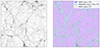Fig. 1. Large-scale structure of the cosmic web. Left panel: density of gas (greyscale) lying along a two-dimensional (75 h−1 cMpc)2, infinitely thin slice across the z = 0 snapshot of TNG100-3. Right panel: same data, but separated into halo (yellow), filament (cyan), and void (purple) substructures according to the metric used in this work.

Cosmological hydrodynamic simulations predict that at low redshifts, most baryons reside in a WHIM phase. This phase is induced through gravitational shock-heating to temperatures of 10⁵–10⁷ K and ∼50ρ_crΩ_baryon densities where ${\rho }_{\mathrm{cr}}=3H_0^2/8\pi G$ is the critical density of the Universe at z = 0, and G is the gravitational constant (Martizzi et al. 2019). The mass fraction in this phase increases from z ∼ 3, may equal that of cold gas by z ∼ 1 (Cen & Ostriker 1999; Medlock & Cen 2021), and encompasses the majority of the missing baryons by z = 0 (Cen & Ostriker 2006; Martizzi et al. 2019). At z = 0, most of the WHIM is predicted to be tied up in filaments (Bregman 2007; Martizzi et al. 2019). The exact evolution of these structures is sensitive to AGN feedback, the modelling of which is of active interest (Haider et al. 2016; Takahashi et al. 2021). Observational evidence for gas in filamentary structures between galaxies, within superclusters, and on larger (10–100 Mpc) scales is growing statistically via Sunyaev-Zel’dovich studies and X-ray emission (see e.g. Tanimura et al. 2019a,b, 2020a,b).

Meanwhile, FRB observations have been used to confirm the existence of the missing baryons (Macquart et al. 2020), and experiments have been proposed to constrain the amount of this matter tied up in the CGM of galaxies versus that in the diffuse IGM (Walters et al. 2019; Ravi 2019; Lee et al. 2022). Simulations have been used to study the DM contribution of the WHIM (Akahori et al. 2016; Medlock & Cen 2021). We are therefore motivated to examine whether the DM contributions of LSS could prove to be a complementary tracer.

3.1. LSS classification in IllustrisTNG

Several different ways to classify LSS have been implemented in the literature (see Libeskind et al. 2018 for a review). Due to the influence of dark matter on LSS formation (Haider et al. 2016), one simple method for identifying cosmic structures uses the local dark matter density of the simulation. We follow this method – as described by Artale et al. (2022), building upon work by Haider et al. (2016) and Martizzi et al. (2019) – to classify TNG300-1 cells. According to this classification scheme, any given cell may be categorised as belonging to a halo, filament, or void using the following metric:

$$\begin{array}{c}\hfill \frac{{\rho }_{\mathrm{c}}}{{\rho }_{\mathrm{cr}}}=\{\begin{array}{cc}<0.1\hfill & \text{for voids,}\hfill \\ 0.1-57\hfill & \text{for filaments,}\hfill \\ >57\hfill & \text{for halos,}\hfill \end{array}\end{array}$$(12)

where ρ_c is the cold dark matter density of the cell, which is provided by the TNG300-1 ‘SubfindDMDensity’ field. The above halo–filament boundary is based on predictions from the Navarro-Frenk-White (NFW) models, and the filament–void boundary is selected to encompass the definition of halos and sheets according to the gravitational potential of each cell (Artale et al. 2022; Martizzi et al. 2019; Forero-Romero et al. 2009). A slice from the simulation coloured according to LSS type can be seen in Fig. 1. Following Artale et al. (2022), Fig. 2 illustrates the amount of matter allocated to each type of structure in the simulation at z = 0 according to our metric. Figure 3 shows the evolution of baryonic mass and electron density within TNG300-1 as a function of LSS and redshift along with previous results provided by Artale et al. (2022).

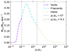Fig. 2. Mass distribution of large-scale structures. Following Artale et al. (2022), the mass distribution within LSS substructures in the z = 0 snapshot of TNG100-3 when binned according to our metric. Yellow, cyan, and purple portions of the curve indicate mass within halos, filaments, and voids, respectively, according to our boundaries (dashed and dot-dashed lines). ρc is the cold dark matter density, and ρcr is the present-day critical density of the Universe.

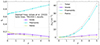Fig. 3. Matter evolution in large-scale structures. Left panel: evolution of the baryonic mass fraction fb in halos (yellow), filaments (cyan), and voids (purple) as a function of redshift in TNG300-1 (solid lines) compared to the results of Artale et al. (2022, dashed lines). For halos, the solid and dashed lines overlap with each other. Right panel: evolution of the total mean electron density ⟨ne⟩ in TNG300-1 (grey line), and in each type of LSS (coloured lines), as a function of redshift.

3.2. Further classification

The practice of reconstructing matter densities along FRB sightlines is a burgeoning field of research. Li et al. (2019), Prochaska & Zheng (2019), and Simha et al. (2020) investigated the environments along sightlines to individual sources using information about spatially proximate galaxies along with various matter-density reconstruction techniques. Lee et al. (2022) propose using similar methods for multiple sources to constrain CGM and IGM parameters. Therefore, tracking the details of collapsed structures along sightlines in IllustrisTNG is also prudent.

TNG provides finely resolved details that are useful for this purpose in the form of ‘sub-halos’, defined as virialised substructures within a dark matter halo (Wechsler & Tinker 2018). In TNG, subhalos are classified using the SUBFIND algorithm (Springel et al. 2001; Nelson et al. 2019). All TNG-simulated galaxies are associated with a subhalo. Through subhalo analysis, any galaxies in proximity to FRB sightlines may therefore be identified. While subhalo identification is not directly provided for individual TNG cells via any field, the ‘Subhalo ID’ for a given cell may be reconstructed by combining the cell’s ‘ParticleID’ field, the entire TNG subhalo catalog, and information supplied by relevant TNG subhalo offset tables⁶.

Not all TNG cells are associated with subhalos. These cells are flagged with a SubhaloID= − 1. Additionally, subhalos do not always contain galaxies. Non-galaxy subhalos include subgalactic, low-mass clumps of baryonic matter, which may be formed via, for example, disc instabilities, which can be distinguished via a flag (Nelson et al. 2019). They may also be differentiated by enforcing cell requirements; for example containing non-zero stellar mass or a certain number of stellar particles⁷. These requirements may vary between TNG runs. In this work, where appropriate, we classify collapsed structures both by considering all subhalos, and by separating these subhalos into bins according to their masses. We therefore note that statistics derived in upcoming sections that consider subhalos of any mass may be influenced by environments containing some subhalos that are small and not well resolved.

4. Methods

As with electron density, the ability to trace sightlines through IllustrisTNG is not directly provided. However, multiple techniques to approximate the environments along sightlines exist. In principle, simulation-agnostic absorption line tools (e.g. TRIDENT; Hummels et al. 2017) should be adaptable for use with IllustrisTNG. In practice, we adapt here the methods first described in Zhang et al. (2021), whereby FRB sightlines are assembled from segments created from each simulation snapshot. To create a given segment, a random subvolume is extracted from the total simulation volume, a line of sight is defined, and the cells closest to this sightline are identified. The ‘true’ line of sight of the FRB is then approximated to propagate through these cells. In Sect. 4.1, we summarise this process and the process of obtaining average electron density and structural information for our segments. Calculating the DM accumulated along an individual segment is described in Sect. 4.2. Finally, Sect. 4.3 describes the process of combining segments to study different DM contributions out to cosmological distances.

4.1. Line-of-sight segments

Following Zhang et al. (2021), we generate a single line of sight segment for a given TNG300-1 snapshot, as follows. Initially, header data detailing snapshot size and redshift are loaded, alongside a matchlist that allows simulation cells to be related to their parent subhalos, as discussed in Sect. 3.2. The physical dimensions of the segment are then defined. A random Cartesian coordinate of the form (0, y, z) is generated as a starting point of the line of sight through the segment. The rectangular extent of the segment – that is, of (205, 0.2,0.2) h⁻¹cMpc, where the x-dimension spans the entire length of the simulation box – is selected so that the segment extends out to 0.1 h⁻¹ cMpc either side of the origin in the y and z directions. The corresponding end-point of the sightline will be (205, y, z) h⁻¹ cMpc.

Once the segment coordinates are defined, all relevant simulation fields are loaded or otherwise created for this snapshot. For clarity, these fields are listed in Table 2. Warm- and cold-phase gas mass fractions are calculated as described in Sect. 2.2. Field values along the segment sightline are obtained from the cells that lie closest to 10 000 linearly spaced bins, each of ∼20 h⁻¹ ckpc in width, which are defined to span the length of the sightline. The LSS type associated with each bin is defined as discussed in Sect. 3.1. We then calculate the number of cells along the segment sightline belonging to each structure type. Electron densities of every cell along the segment sightline are calculated as discussed in Sect. 2.2. These are averaged to obtain the average total electron density traversed along the segment. The average electron densities associated with each LSS type across the segment sightline are also calculated separately.

Additionally, Subhalo IDs associated with cells along the sightline are identified as discussed in Sect. 3.2. Unique subhalos are stored, and all bins along the segment associated with these subhalos are identified. In this way, all DM attributed to these subhalos may also be calculated. The sightline’s coordinates of closest approach to the central positions of these subhalos are also stored for further analysis. An example segment can be seen in the left panel of Fig. 4. An example impact parameter analysis can be seen in the right panel of Fig. 4.

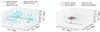Fig. 4. Tracing structure along sightlines. Left panel: a (205, 0.2, 0.2) h−1 cMpc line of sight segment traversing a TNG snapshot at z = 0. The grey line indicates the sightline through the segment. Blue squares projected onto the (xy, yz, xz) planes represent the number density of all cells within the segment in the (x, y, z) directions. Dots coloured according to their LSS type represent the central locations of all cells identified as closest to one of the 10 000 bins along the sightline. The sightline is approximated to traverse these cells due to the Voronoi tessellation of the simulation. Right panel: a second sightline complete with the subhalo it traverses and the impact parameter measured between the sightline and subhalo.

4.2. DM within a segment

Using the information recorded for each segment, the DM accumulated along its line of sight can be calculated. We compute the total DM along a given segment sightline by converting the continuous Eq. (1) into a discrete sum over its bins, assuming a negligible redshift change over the length of a snapshot:

$$\begin{array}{c}\hfill \mathrm{DM}=\stackrel{\sim }{\mathrm{DM}}/(1+z),\end{array}$$(13)

where $\stackrel{\sim }{\mathrm{DM}}$ is the total DM along the segment’s sightline in its rest frame,

$$\begin{array}{c}\hfill \stackrel{\sim }{\mathrm{DM}}=\sum _{n=1}^{10000}\frac{\mathrm{d}\mathrm{DM}}{\mathrm{d}l}{|}_n\times \mathrm{d}l.\end{array}$$(14)

In Eq. (14), (d DM/dl)_n = n_e is the physical electron density of the nth bin, as described by Eq. (7), and dl = adη is the physical distance increment of propagation through the bin, where a is the scale factor at the redshift of the segment, and dη is the comoving distance increment, which is equal to the bin width in comoving IllustrisTNG units⁸. It therefore follows that the DM accumulated by a limited portion of a sightline traversing a particular subhalo can be calculated by constraining Eq. (14) to only those bins associated with its specific Subhalo ID.

4.3. Combining DM from different segments

Following Zhang et al. (2021), to form complete sightlines between sources at redshift z and an observer at z = 0, we exploit the lack of redshift evolution within snapshots, approximating them as infinitesimally narrow redshift slices in order to convert Eq. (3), the continuous theoretical integral for DM_cos, into a discrete cumulative sum over our snapshots, which we denote ${\mathrm{DM}}_{\mathrm{total}}^{\mathrm{TNG}}$:

$$\begin{array}{cc}& {\mathrm{DM}}_{\mathrm{total}}^{\mathrm{TNG}}(z_{i+1})={\mathrm{DM}}_{\mathrm{total}}^{\mathrm{TNG}}(z_i)\hfill \\ \hfill & +\frac{1}{2}(\frac{\mathrm{d}{\mathrm{DM}}_{\mathrm{TNG}}}{\mathrm{d}z}{|}_{z_i}+\frac{\mathrm{d}{\mathrm{DM}}_{\mathrm{TNG}}}{\mathrm{d}z}{|}_{z_{i+1}})(z_{i+1}-z_i),\hfill \end{array}$$(15)

where z_i is the redshift of each snapshot, ${\mathrm{DM}}_{\mathrm{total}}^{\mathrm{TNG}}{(z)|}_{z=0}=0$, and for a given segment of a given snapshot,

$$\begin{array}{c}\hfill \frac{\mathrm{d}{\mathrm{DM}}_{\mathrm{TNG}}}{\mathrm{d}z}{|}_{z=z_i}=\frac{c{n}_{\mathrm{e}}(z_i)}{H_0{(1+z_i)}^2\sqrt{{\mathrm{\Omega }}_{\mathrm{m}}{(1+z)}^3+{\mathrm{\Omega }}_{\mathrm{\Lambda }}}},\end{array}$$(16)

where n_e is the average electron density computed as described in Sect. 4.1. Additionally, if any cell along the segment sightline is associated with a dark matter subhalo (see Sect. 3.2) then we consider the subhalo to have been traversed by the sightline. By recording the number of unique subhalos traversed by each segment, the number of subhalos N_sub traversed as a function of redshift for a single sightline may then be calculated similarly to Eq. (15), using the following equation:

$$\begin{array}{cc}& N_{\mathrm{sub}}(z_{i+1})=N_{\mathrm{sub}}(z_i)\hfill \\ \hfill & +\frac{1}{2}(\frac{\mathrm{d}{N}_{\mathrm{sub}}}{\mathrm{d}z}{|}_{z_i}+\frac{\mathrm{d}{N}_{\mathrm{sub}}}{\mathrm{d}z}{|}_{z_{i+1}})(z_{i+1}-z_i),\hfill \end{array}$$(17)

with the initial condition N_sub(z)|_z = 0 = 0, and where dN_sub/dz is the number of subhalos traversed by a given segment.

Although full TNG300-1 snapshots extend out to z = 12, and FRBs may be detectable by current instruments out to at least z = 10 (Zhang 2018), the ionisation information that informs our electron densities may be inaccurate at z > 6 (Nelson et al. 2018). We therefore generated segments as discussed in Sect. 4.1 for only the snapshots listed in Table 1, which extend out to z = 5. We calculated N_sub and the cosmological ${\mathrm{DM}}_{\mathrm{total}}^{\mathrm{TNG}}$ for these, and calculated the portions of DM acquired only from individual LSS types (${\mathrm{DM}}_{\mathrm{halos}}^{\mathrm{TNG}}$, ${\mathrm{DM}}_{\mathrm{filaments}}^{\mathrm{TNG}}$, ${\mathrm{DM}}_{\mathrm{voids}}^{\mathrm{TNG}}$) by substituting n_e in Eq. (16) with the average electron densities associated only with their corresponding structures. Following Zhang et al. (2021), we created a total of 5125 unique segments of (205, 0.2,0.2) h⁻¹ cMpc in dimension for each snapshot; these are randomly sampled to create 10 000 000 individual FRB lines of sight. We also observe the convention of constructing our FRB sightlines along the x-axes of our snapshots due to computing constraints (Jaroszynski 2019; Zhang et al. 2021). Including sightlines constructed along all three axes would better sample the entire simulation, and hence improve results. In principle, adapting the absorption line tool TRIDENT (Hummels et al. 2017) for use with IllustrisTNG, perhaps in conjunction with techniques discussed in Batten et al. (2021) for bridging gaps between simulation snapshots, could prove to be another powerful way to study not just average, but individual, sightlines across the full breadth of the IllustrisTNG simulation suite.

Figure 5 presents normalised histograms showing the evolution of the distribution of ${\mathrm{DM}}_{\mathrm{total}}^{\mathrm{TNG}}$ values calculated for our sightlines, and for their LSS contributions, as a function of redshift. We find that ${\mathrm{DM}}_{\mathrm{filaments}}^{\mathrm{TNG}}$ and ${\mathrm{DM}}_{\mathrm{voids}}^{\mathrm{TNG}}$ are both best fit by lognormal distributions⁹ of the form

$$\begin{array}{c}\hfill P(y,a)=\frac{1}{s}\frac{1}{ay\sqrt{2\pi }}exp(-\frac{{ln}^2(y)}{2a^2}),\end{array}$$(18)

and that ${\mathrm{DM}}_{\mathrm{halos}}^{\mathrm{TNG}}$ can be approximated using the positive range of a log-logistic distribution¹⁰ fitted to the natural logarithm of the DM data:

$$\begin{array}{c}\hfill P(y,a)=\frac{1}{s}\frac{a{y}^{a-1}}{{(1+y^a)}^2}.\end{array}$$(19)

In each case, a refers to the distribution’s shape parameter, and

$$\begin{array}{c}\hfill y=\frac{(x-l)}{s}\mathrm{where}\{\begin{array}{cc}x=\text{DM}\hfill & \text{for voids, filaments,}\hfill \\ x=ln(\text{DM})\hfill & \text{for halos,}\hfill \end{array}\end{array}$$(20)

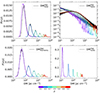Fig. 5. FRB DM evolution with redshift. Clockwise from top left: histogram of the probability distributions (solid coloured lines) of the total cosmological DM (${\mathrm{DM}}_{\mathrm{total}}^{\mathrm{TNG}}$), and contributions from large-scale structures (${\mathrm{DM}}_{\mathrm{halos}}^{\mathrm{TNG}}$, ${\mathrm{DM}}_{\mathrm{filaments}}^{\mathrm{TNG}}$, ${\mathrm{DM}}_{\mathrm{voids}}^{\mathrm{TNG}}$) for FRBs originating at various redshifts (see Table 1 and colour bar), calculated for TNG300-1. For comparison, grey lines are new data drawn from fits to these LSS distributions. These new data are combined to create the comparison histograms for ${\mathrm{DM}}_{\mathrm{total}}^{\mathrm{TNG}}$. The slight mismatch between our low-redshift TNG data and drawn ${\mathrm{DM}}_{\mathrm{total}}^{\mathrm{TNG}}$ values arises due to the fact that our fits slightly overestimate the probability of sightlines containing very high (≳103 pc cm−3) ${\mathrm{DM}}_{\mathrm{halos}}^{\mathrm{TNG}}$ contributions at low redshifts.

with shifting parameters l and scaling parameters s, respectively. The best-fit parameters for each distribution at each redshift are provided in Table A.1. Histograms of data drawn from these fits are included in Fig. 5 for comparison purposes. The draws from the void and filamentary fits are a good match to the TNG data distributions, while draws from the halo fits are a relatively good match, but slightly overestimate the probability of low-redshift sightlines containing high (≳10³ pc cm⁻³) ${\mathrm{DM}}_{\mathrm{halo}}^{\mathrm{TNG}}$ contributions.

Using our distributions, we calculate various statistics (mean, median, standard deviation) for the relationship between ${\mathrm{DM}}_{\mathrm{total}}^{\mathrm{TNG}}$ and redshift. In Fig. 6, we compare these to similar results reported in the literature. These comparisons are further discussed in Sect. 6.1. In Fig. 7 (left), we compare the average behaviours of ${\mathrm{DM}}_{\mathrm{halos}}^{\mathrm{TNG}}$, ${\mathrm{DM}}_{\mathrm{filaments}}^{\mathrm{TNG}}$, and ${\mathrm{DM}}_{\mathrm{voids}}^{\mathrm{TNG}}$. We present more detailed breakdowns of the fractional contributions to FRB DM from each type of large-scale structure as a function of redshift in Fig. 7 (right), and provide computed values at our redshift intervals for all measurements in Table A.2.

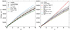Fig. 6. FRB DM evolution with redshift continued. Both panels: average total DM–z relationship derived for TNG300-1. The mean (solid grey line), median (dotted grey line), and standard deviation (shaded grey region) around the mean of ${\mathrm{DM}}_{\mathrm{total}}^{\mathrm{TNG}}$ values calculated for our sightlines are shown. Left panel: compared to ⟨DMcosmic⟩ (dashed black line), and the results of analytical studies from the literature (dashed coloured lines). Right panel: compared to results derived from other cosmological simulations in the literature (dashed coloured lines).

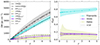Fig. 7. Redshift evolution of DM contributions as a function of large-scale structure. Left panel: mean, median, and standard deviation around the mean of the DM–redshift relationship for TNG300-1 halos (${\mathrm{DM}}_{\mathrm{halos}}^{\mathrm{TNG}}$; yellow), filaments (${\mathrm{DM}}_{\mathrm{filaments}}^{\mathrm{TNG}}$; cyan), and voids (${\mathrm{DM}}_{\mathrm{voids}}^{\mathrm{TNG}}$; purple) derived using our metric. These are compared to the ⟨DMcosmic⟩ subcomponents (see Sect. 6.1): ⟨DMIGM⟩ (dashed black line) and ⟨DMCGM⟩ (dot-dashed black line). Right panel: means (coloured lines) and standard deviations (shaded regions) of the equivalent fractional DM contributions ⟨fDM⟩ accumulated due to traversing each type of structure by our FRBs originating at given redshifts.

5. Results

In previous sections, we review the ingredients and methods required to approximate both LSS and DM for IllustrisTNG. Together, these elements may be combined to provide detailed insight into the redshift-evolving impact of cosmological large-scale structures on FRB signals. In this section, we present the results of our analysis.

5.1. LSS analysis

Figure 5 presents individually normalised distributions for ${\mathrm{DM}}_{\mathrm{total}}^{\mathrm{TNG}}$ values accumulated along our sightlines by FRBs originating at various redshifts. Individually normalised distributions for the contributions to the total DM by each type of LSS (${\mathrm{DM}}_{\mathrm{halos}}^{\mathrm{TNG}}$, ${\mathrm{DM}}_{\mathrm{filaments}}^{\mathrm{TNG}}$, ${\mathrm{DM}}_{\mathrm{voids}}^{\mathrm{TNG}}$) are also shown. The similarity between the total and filamentary DM distributions (Fig. 5 top left, bottom left) is immediately apparent, indicating that for most sightlines the filamentary contribution dominates DM. The filament and halo distributions also display the widest DM ranges, and high-DM tails, including those for FRBs originating at low redshifts. This behaviour indicates that the ionised electron distributions in halo and filament environments may significantly vary between FRB sightlines, and that in rare instances, an FRB may propagate through a region of much higher electron density, which will contribute large amounts of observed DM. In contrast, the narrower distributions of the void components indicate that voids contribute a smaller range of possible DM values to FRB sightlines, suggesting that voids are environments that remain generally more homogeneous from one sightline to another.

The differing behaviours of the contributions to DM by each type of LSS as a function of redshift are quantified using various statistics presented in Fig. 7 and Table A.2. In Fig. 7 (left), we compare the evolution of the average total observed DM from TNG, $⟨{\mathrm{DM}}_{\mathrm{total}}^{\mathrm{TNG}}⟩$, to the evolution of its LSS subcomponents, $⟨{\mathrm{DM}}_{\mathrm{halos}}^{\mathrm{TNG}}⟩$, $⟨{\mathrm{DM}}_{\mathrm{filaments}}^{\mathrm{TNG}}⟩$, and $⟨{\mathrm{DM}}_{\mathrm{voids}}^{\mathrm{TNG}}⟩$. Here, the dominance of the filamentary contribution to the average FRB sightline is more apparent. It can be seen that filaments contribute an increasingly large portion of DM to the total for FRBs originating at higher redshifts, while halos and voids contribute to a lesser extent. We find that for FRBs originating at z = 0.1 versus z = 5, the average contributions to DM from halos, filaments, and voids will grow from ∼[13.64/65.82/13.13] pc cm⁻³ to ∼[327.61/3494.53/563.02] pc cm⁻³, respectively. The standard deviations of these components quantify the DM variability due to each type of LSS along our sightlines. It can be seen that the largest DM scatter arises because of the material in halos; filaments then show less DM scatter, followed by voids, which show very little scatter. A more detailed breakdown of the evolution of these average components can be found in Table A.2.

In Fig. 7 (right), we quantify the relative evolution of our LSS DM components as a function of redshift using their average fractional contributions to the total DM. We again see that $⟨{\mathrm{DM}}_{\mathrm{filaments}}^{\mathrm{TNG}}⟩$ is the dominant contribution to $⟨{\mathrm{DM}}_{\mathrm{total}}^{\mathrm{TNG}}⟩$, and that, on average, the fraction of DM accumulated from filaments, $⟨f_{\mathrm{filaments}}^{\mathrm{DM}}⟩$, rises from ∼71% to ∼80% for an FRB originating at z = 0.1 versus z = 5, respectively. Meanwhile, the average fraction accumulated from halos, $⟨f_{\mathrm{halos}}^{\mathrm{DM}}⟩$, halves, from ∼15% to ∼8%. The average fractional contribution from voids, $⟨f_{\mathrm{voids}}^{\mathrm{DM}}⟩$, remains relatively consistent, to within ∼1%, regardless of source redshift. Here too, the significant scatter in ${\mathrm{DM}}_{\mathrm{halos}}^{\mathrm{TNG}}$ and ${\mathrm{DM}}_{\mathrm{filaments}}^{\mathrm{TNG}}$ can be seen, and all calculated values can be found in Table A.2. These results support previous predictions that denser structures, such as galaxy groups and clusters, may be the major contributors to any observed variance between sightlines in FRB DMs (Prochaska & Zheng 2019; Zhu & Feng 2021; Connor & Ravi 2022).

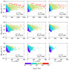Fig. 8. Collapsed structures traversed by our segments. Each panel: scatter points indicating the distributions in the impact parameter (b⊥, sub)–accumulated dispersion measure (DMsub) parameter space for any subhalos considered traversed by our segments, in the snapshot of redshift z described in the legend. Each scatter point colour is determined using its subhalo mass Msub according to the mass bin ranges described by the colour bar. The total number of subhalos Nsub traversed by all segments within a given snapshot is provided in the legend.

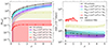Fig. 9. Collapsed structures traversed with redshift. Left panel: statistics (mean, standard deviation) describing the average number of subhalos traversed by FRB sightlines out to given redshifts within TNG300-1. Black lines and grey shaded regions describe the total number of subhalos traversed; coloured lines and shaded regions describe the number of subhalos when binned by mass according to the mass bins of Fig. 8. Right panel: statistics (median, interquartile range) describing the average impact parameters between our sightlines and these structures within each snapshot. Overplotted crosses are the impact parameters between observed FRBs and galaxies as calculated by Connor & Ravi (2022), Connor et al. (2020), and Prochaska et al. (2019a).

5.2. Subhalo analysis

Table A.3 quantifies the number of unique subhalos intersected by our segments at various redshifts. We provide the total number of subhalos intersected for a given snapshot, and bin these according to their masses. Figure 8 visualises these data, along with the impact parameters b_⊥, sub and accumulated dispersion measures DM_sub, which are associated with these intersections. It is immediately apparent that the general trend is towards fewer subhalo intersections at lower redshifts, which is presumably due to the merging of lower-mass subhalos to form higher-mass subhalos over cosmic time. We can also see that larger potential impact parameters are possible for low-redshift subhalos, presumably due to increased sizes. In addition, for a given redshift, higher-mass subhalos generally contribute larger values of DM_sub, and allow larger potential impact parameters, indicating potentially larger radii. We anticipate that the exact cutoffs in DM_sub–b_{⊥,  sub} -space for subhalos of different mass bins are governed by the radius–density profile of these subhalos.

We quantify the average evolution of these intersections for complete FRB sightlines as a function of redshift in Fig. 9 and Tables A.4 and A.5. The left panel of Fig. 9 and Table A.4 detail the average number of subhalos that an FRB originating at a given redshift will traverse according to Eq. (17). We present the mean and standard deviations calculated for our 10 000 000 sightlines. The right panel of Fig. 9 and Table A.5 detail the average impact parameters that we measure between our segments and these subhalos at the redshifts of our snapshots. Due to the non-Gaussianity we observe for these distributions, we present median, interquartile range (IQR), and interpercentile range (IPR) values calculated for these data. For comparison, we overplot derived positions in impact parameter–redshift space for a number of observed FRBs that are considered likely to have intersected galaxies including M31 and M33 according to Prochaska et al. (2019a), Connor et al. (2020), and Connor & Ravi (2022). Where not otherwise provided by the literature, we converted the impact parameters for these galaxies from physical to comoving distances using their preferred redshifts, which we obtained using the NASA Extragalactic Database (NED). Where a galaxy was reported to have a blueshift, z = 0 was used in the conversion process. In both subplots of Fig. 9, we present the statistics obtained when considering all subhalos traversed by our sightlines, and those we obtain when considering subhalos binned by mass according to the bins in Fig. 8. We note that we only provide impact parameter statistics for a given mass bin and redshift in Table A.5 when the total number of subhalos traversed by segments in the snapshot for this mass bin is ≥40 (see Table A.3).

The left panel of Fig. 9 shows that, on average, FRBs originating from beyond 0.5 < z < 0.7 will intersect at least one subhalo of any mass during propagation. The total number of subhalos that are on average traversed will increase from ⟨N_sub⟩≃1.8 for an FRB originating at z = 1 to ⟨N_sub⟩≃12.4 for an FRB originating at z = 5. By studying these intersected subhalos according to their masses, we see that the traversed subhalos are dominated by those of mass M_sub = [10⁸, 10¹²] h⁻¹ M_⊙. On average, less than one subhalo of mass M_sub ≥ 10¹² h⁻¹ M_⊙ will be traversed, even by an FRB originating at z = 5. When comparing the relative behaviours of the mass-binned halos as a function of redshift, one sees that FRBs originating at z ≲ 3 are more likely to traverse higher-mass subhalos (M_sub = [10¹⁰, 10¹²] h⁻¹ M_⊙), but for FRBs originating at z ≳ 4, the most commonly intersected collapsed structures are of lower mass (M_sub = [10⁸, 10¹⁰] h⁻¹ M_⊙), with the transition occurring at around z ∼ 3.8. This transition in the encounter rates of lower-mass versus higher-mass subhalos likely stems from the fact that the population of less massive subhalos decreases towards later times as a result of continuous mergers.

By studying the impact parameters between our sightlines and mass-binned traversed subhalos in Fig. 9 (right), it can be seen that the average impact parameter between our sightlines and subhalos increases with mass, from a median of b_⊥, sub ≃ 36.1 h⁻¹ ckpc for subhalos of mass M_sub = [10⁸, 10¹⁰] h⁻¹ M_⊙ to b_⊥, sub ≃ 950 h⁻¹ ckpc for subhalos of mass M_sub = [10¹⁴, 10¹⁶] h⁻¹ M_⊙. These average impact parameters remain relatively consistent for subhalos with masses M_sub = [10⁸, 10¹⁴] h⁻¹ M_⊙, regardless of the redshift of intersection. However, the average impact parameter measured when considering subhalos of any mass falls after z > 1. This is presumably due to a deficit of subhalos of the highest masses (M_sub > 10¹⁴h⁻¹ M_⊙) at higher redshifts, which have not yet had time to form within the TNG300-1 box.

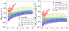Fig. 10. DM accumulated within individual snapshots due to traversing collapsed structures. Left panel: statistics (median, interquartile range) describing the average $\stackrel{\sim }{\mathrm{DM}}$ accumulated within snapshots by sightlines traversing our subhalos in the rest frames of the snapshots, and therefore the rest frames of the subhalos. Right panel: these values weighted by redshift, effectively describing the average DM that would be observed by an observer at z = 0 due to these subhalos. Colours indicate the mass ranges described in Fig. 9.

Finally, we quantify the average DMs accumulated as our lines of sight traverse the subhalos in Fig. 10 and Table A.6. The left panel of Fig. 10 details the average dispersion measure that will be accumulated by traversing any subhalos at a given redshift in the rest frame of the subhalos, ${\stackrel{\sim }{\mathrm{DM}}}_{\mathrm{sub}}$ (see also Sect. 4.2). The right panel of Fig. 10 and Table A.6 detail the average DM that will be observed due to traversing subhalos at these redshifts. Here too, we present statistics obtained when considering traversed subhalos of any mass, and when considering subhalos binned by their masses. It can be seen that although ${\stackrel{\sim }{\mathrm{DM}}}_{\mathrm{sub}}$ increases with redshift in all cases, this increase is greatly suppressed when considering observed DM, due to the (1 + z)⁻¹ factor. Again, we only provide DM statistics for a given mass bin and redshift in Table A.6 when the total number of subhalos traversed by segments in the snapshot for this mass bin is ≥40 (see Table A.3).

6. Discussion

The study of matter distributions in difficult-to-observe phases is a burgeoning field of research. Observationally, Sunyaev-Zel’dovich and X-ray studies are already being used (Tanimura et al. 2019a,b, 2020a,b); as are cosmological hydrodynamic simulations, to within the constraints imposed, by for example, their feedback models. In the future, large galaxy catalogues provided by surveys such as LSST (Ivezić et al. 2019) might also be useful in conjunction with matter density reconstruction techniques (see e.g. Wang et al. 2009, 2012, 2016) for reconstructing large volumes of LSS. Fast radio bursts, with their isotropic sky distribution (Petroff et al. 2022) and the insight they provide into the ionised environments that they traverse, may yet provide a valuable way to augment such techniques, and aid our understanding of the ionised matter distribution of the Universe.

In view of this, we investigated the evolution with redshift of the cosmological DM contribution; the contributions of its constituent halos, filaments, and voids; the likelihood of intercepting foreground collapsed structures; and the impact parameters and DM contributions associated with these interceptions, for FRBs within TNG300-1. In this section, we compare our results to previous investigations using different analytical, empirical, and theoretical methods, different simulations and LSS classification schemes, and real FRB observations.

6.1. LSS analysis

In Fig. 6, we compare $⟨{\mathrm{DM}}_{\mathrm{total}}^{\mathrm{TNG}}⟩$, the average total DM that the cosmological component will contribute to an FRB originating at a given redshift according to our simulation to similar results from the literature. In most cases, the results appear reasonably consistent, with many remaining within one standard deviation of the TNG result out to z = 4.

Using the publicly available FRUITBAT repository (Batten 2019; Batten et al. 2021)¹¹, we reproduce the results of Ioka (2003), Inoue (2004), and Zhang (2018) in Fig. 6 (left). These are analytical estimates that approximate Eq. (5), and thus DM, using different IGM baryon fractions, f_d, and free electron fractions, f_e, and assume these to be constant with redshift (see Batten et al. 2021 for a brief review). These values evolve with redshift in TNG (see Eq. (7)), which will account for some of the differences between the analytical results and our analysis. Conversely, the evolution of ⟨DM_cosmic⟩ with redshift (see e.g. Prochaska & Zheng 2019, Macquart et al. 2020), which we recreate using the public FRB GitHub repository (Prochaska et al. 2019b, 2023)¹² for Fig. 6 (left), is derived by combining theoretical predictions and empirical techniques, and allows for redshift-evolving IGM baryon and ionisation factors; it appears much closer to our result.

We also compare our results to the most probable DM–z relationships obtained using various cosmological simulations in Fig. 6 (right). These include the medium-resolution Magneticum Pathfinder simulation (Dolag et al. 2015), the original Illustris simulation (Jaroszynski 2019), the RAMSES simulation (Zhu & Feng 2021), the EAGLE simulation (Batten et al. 2021), and IllustrisTNG, when interpolating the results of Zhang et al. (2021). It is notable that our recreation of the Zhang et al. (2021) result (see Fig. 6 (right), yellow dashed line), which we achieve by interpolating their fits, yields systematically lower DMs as a function of redshift than our own result, despite both being derived using the same run of the same simulation (TNG300-1). We posit that these differences arise for two reasons. Firstly, a systematic shift towards lower DMs in the peak of the Zhang et al. (2021) fitted distributions compared with their data distributions can be seen when comparing each for a given redshift. Secondly, Zhang et al. (2021) elect to discard cells containing measurable star formation during their DM calculations, whereas we apply a correction factor (see Eq. (8)) to these cells, and still include some portion of their material in our calculations. Minor differences between our result and the majority of the other simulations likely arise because of technical differences and differences in the underlying assumptions that inform the simulations. These could include the sizes, resolutions, and AGN feedback models of the simulations, and the exact values of the cosmological parameters that they are initialised with.

All considered, the fact that the majority of the other curves lie within one standard deviation of our result demonstrates a broad consistency with the literature, albeit highlighting the non-negligible effect that underlying cosmological parameters and galaxy evolution mechanisms have on the true DM–redshift relationship.

In the left panel of Fig. 7, we compare the evolution of $⟨{\mathrm{DM}}_{\mathrm{total}}^{\mathrm{TNG}}⟩$ to the evolution of its large-scale structure subcomponents, $⟨{\mathrm{DM}}_{\mathrm{halos}}^{\mathrm{TNG}}⟩$, $⟨{\mathrm{DM}}_{\mathrm{filaments}}^{\mathrm{TNG}}⟩$, and $⟨{\mathrm{DM}}_{\mathrm{voids}}^{\mathrm{TNG}}⟩$. For reference, we plot these against another interpretation of the cosmological DM component. In this figure, ⟨DM_cosmic⟩, and its subcomponents, ⟨DM_CGM⟩¹³ and ⟨DM_IGM⟩, are calculated using the public FRB GitHub repository. The value ⟨DM_CGM⟩ describes the average DM contributed to ⟨DM_cosmic⟩ by ionised material residing within the CGM of any galactic halos that lie along FRB sightlines as a function of redshift, and is computed using the Aemulus Halo Mass Function (McClintock et al. 2019). Thus, the value ⟨DM_IGM⟩, which is defined as ⟨DM_cosmic⟩ − ⟨DM_CGM⟩, must attribute any remaining DM to matter within the diffuse IGM, but outside of foreground galactic halos. When compared with our derived values, it can be seen that ⟨DM_CGM⟩ consistently accounts for a larger portion of ⟨DM_cosmic⟩ than the portion of $⟨{\mathrm{DM}}_{\mathrm{total}}^{\mathrm{TNG}}⟩$ contributed by $⟨{\mathrm{DM}}_{\mathrm{halos}}^{\mathrm{TNG}}⟩.$ This likely results from the Aemulus Halo Mass Function incorporating all matter classified as belonging to halos according to our metric, as well as some of the denser matter lying closer to these halos, which we might classify as belonging to filaments. Likewise, it can be seen that ⟨DM_IGM⟩ consistently contributes a smaller portion of ⟨DM_cosmic⟩ than the portion of $⟨{\mathrm{DM}}_{\mathrm{total}}^{\mathrm{TNG}}⟩$ contributed by $⟨{\mathrm{DM}}_{\mathrm{filaments}}^{\mathrm{TNG}}⟩$, presumably because it includes only the less dense portion of the matter which we classify as filamentary, along with any matter we classify as belonging to voids.

Zhu & Feng (2021) previously used the RAMSES simulation to investigate the DM contributions of large-scale structures in the range 0 < z < 1, assuming different definitions for large-scale structure types. These authors report values at z = 0, which we can compare to our results at z = 0.1. Assuming equivalence between the definition of nodes provided by Zhu & Feng (2021) and our definition of halos, and that our definition of filaments encompasses Zhu & Feng (2021) filaments and walls, the results of Zhu & Feng (2021) translate to ∼23.5%, ∼61.4%, and ∼15% of cosmological DM being attributed to halos, filaments, and voids, respectively, at z = 0. These values are consistent to within one standard deviation of our results at z = 0.1.

Conversely, Akahori et al. (2016) previously studied the contributions to DM by large-scale structures out to z ∼ 5 using the ΛCDM universe simulations. These authors adopt a different classification scheme, defining their structures as voids, sheets, filaments (which they also define as the WHIM), and clusters according to gas temperature (T < 10⁴ K; 10⁴ K < T < 10⁵ K; 10⁵ K < T < 10⁷ K; and T > 10⁷ K respectively). Their work yields different results when compared with our Table A.2. While the fractional contributions to total DM by matter that we classify as halos and Akahori et al. (2016) classify as clusters both decrease with redshift, our filamentary fraction grows over the range 0.1 < z < 5, and our void fraction decreases. In Akahori et al. (2016), these two contributions evolve in the opposite direction. Akahori et al. (2016) voids increase their relative DM contribution with redshift, overtaking the DM contributed by their filaments by z ∼ 2. By z ∼ 5, voids exceed filaments in their fractional contribution to total DM by a factor of > 2, and by over ∼ 1000 pc cm⁻³. This 1000 pc cm⁻³ DM excess between filaments and voids is larger than the average DM contribution by all TNG matter that we classify as belonging to voids using our metric. Assuming that our definition of filaments encompasses the Akahori et al. (2016) definitions of both filaments and sheets (see e.g. Martizzi et al. 2019, who show that filaments defined using local dark matter density are equivalent to filaments plus sheets when defined using the tidal tensor method) may reduce this discrepancy to some extent. However, this still does not reconcile the two sets of results. As with our comparison of $⟨{\mathrm{DM}}_{\mathrm{total}}^{\mathrm{TNG}}⟩$ to the literature, the root of the discrepancy between the trends for our LSS contributions likely derives from fundamental differences between our simulations and those in the literature (e.g. underlying galaxy feedback models), and from differences in the methods used for constructing FRB sightlines and our categorisation of LSS according to gravitational collapse rather than temperature.

When analysing the relative contributions to DM accumulated from our different LSS types, the relatively low variance in the DM contributed by voids between sightlines presents an interesting possibility. Walters et al. (2018) previously showed that the constraining power of FRBs on cosmological parameters is limited by the inhomogeneity of the IGM from one sightline to another, and that minimising this variance may be necessary in order to use FRBs to measure the dark energy equation of state. It therefore follows that, if a sample of FRBs propagating along low-structure sightlines traversing only (or mostly) void material could be assembled, these low-variance sources might offer the ability to obtain tighter cosmological constraints than those obtained when using the full FRB population. This idea has been touched on by Baptista et al. (2023), who, building on the P(DM|z) model of Macquart et al. (2020), parameterised the halo gas contribution to its deviation from a Gaussian in terms of a fluctuation parameter, F. While investigating the degeneracy of this parameter with H₀, these authors note that the low DM end of the P(DM|z) distribution is less affected by the choices of F and H₀, implying that lower-structure sightlines (e.g. through voids) may better constrain H₀.

As the measurable parameter for observed FRBs is total DM, to obtain such a sample, one would have to inventively select probable low-structure-sightline FRBs from the overall population. Potential methods might include selecting well-localised FRBs with observed DMs that are lower than expected when considering their P(DM|z) redshift distributions (see e.g. Walker et al. 2020), or using, for example, photometric techniques (Simha et al. 2021) to identify structureless sightlines. Such work could also potentially help to constrain the baryon distribution within voids.

6.2. Subhalo analysis

In Fig. 9 (left) and Table A.4, we quantify the average number of collapsed structures traversed by an FRB originating at a given redshift, according to our simulations. In Fig. 9 (right) and Table A.5, we quantify the average impact parameters b_⊥ that we measure between any collapsed structures traversed by our sightlines, and the sightlines that traversed them, at the redshifts of our snapshots. For reference, we compared these results to real observational FRB data. Prochaska et al. (2019a) studied the halo gas of a galaxy intersected by an ASKAP-localised FRB, and Connor et al. (2020) reported a single FRB that intersects regions of both M33 and M31. Additionally, Connor & Ravi (2022) discuss unlocalised, non-repeating, CHIME-detected FRBs, which they deem likely to have intersected galaxies (but unlikely to have passed directly through their discs) during their propagation through the IGM. The FRB–galaxy intersection discussed by Prochaska et al. (2019a) occurs at z ∼ 0.37 with the ∼10¹² h⁻¹ M_⊙ galaxy FG-181112 at b_⊥ ∼ 27 h⁻¹ ckpc. This impact parameter lies outside of the IQR (=[39.88, 128.27] h⁻¹ ckpc), which we measure at z = 0.4 when considering impact parameters between all subhalos and our sightlines, and when considering impact parameters to subhalos of mass M_sub = [10¹², 10¹⁴] h⁻¹ M_⊙ (=[184.85, 438.88] h⁻¹ ckpc). This intersection additionally lies outside of the 10th to 90th percentiles (=[112.76, 663.54] h⁻¹ ckpc), which we measure for intersections with subhalos of mass M_sub = [10¹², 10¹⁴] h⁻¹ M_⊙, though it lies within these percentiles when considering subhalos of any mass. These results support the finding by Prochaska et al. (2019a) that this is a particularly rare intersection event (which they place at a probability of ∼0.5%).

Of the 28 FRB–galaxy impact parameters discussed by Connor et al. (2020) and Connor & Ravi (2022), all are associated with galaxies that lie at z ≃ 0. Of these 28 impact parameters, we find that 19 lie within the IQR (=[41.33, 131.86] h⁻¹ ckpc) that we measure when considering the impact parameters between subhalos of all masses and our sightlines at z = 0. Additionally, we find that 26 of these 28 lie between the 10th and 90th percentiles (=[23.06, 303.08] h⁻¹ ckpc) that we measure for our impact parameters when considering subhalos of all masses. The FRB–galaxy impact parameters that lie outside these ranges are associated with FRB20190430B (Connor & Ravi 2022) and FRB191108 (Connor et al. 2020), in their purported intersections with the galaxies NGC6015 and M33 at b_⊥ ≃ 12.9 h⁻¹ ckpc and b_⊥ ≃ 12.2 h⁻¹ ckpc respectively. As demonstrated by Prochaska et al. (2019a), FRBs may impact intervening galaxies at closer distances on rare occasions, and therefore we see no discrepancy between our analysis and this result. However, we note that every galaxy considered by Connor & Ravi (2022) is reported to have M_vir > 10¹² h⁻¹ M_⊙, placing them in our [10¹², 10¹⁴] h⁻¹ M_⊙ subhalo mass bin. Many of the Connor & Ravi (2022)b_⊥ values fall outside our measured ranges when considering subhalos in this mass bin alone.

Figure 10 and Table A.6 quantify the average dispersion measures accumulated within individual snapshots by our sightlines due to traversing these subhalos. The left panel of Fig. 10 presents the average dispersion measures ${\stackrel{\sim }{\mathrm{DM}}}_{\mathrm{sub}}$ accumulated within snapshots of given redshifts by our segments due to traversing their subhalos, in the rest frame of the subhalos. We find these increase with redshift, both when considering all traversed subhalos, and when considering subhalos binned by mass. The right panel of Fig. 10 presents the average observed dispersion measures DM_sub due to these intersections. We find the observed DMs to be strongly suppressed as a function of redshift by the (1 + z)⁻¹ factor. These trends generally align well with the literature that examines the DM contributions of FRB host galaxies, such as Jaroszyński (2020), Zhang et al. (2020), and Kovács et al., (in prep.), who also report increasing, albeit suppressed, average DM_host contributions as a function of redshift. The works report systematically larger average DM_host contributions (of the order of tens to hundreds of pc cm⁻³; Jaroszyński 2020; Zhang et al. 2020) than our average DM_sub values (which have medians of the order of DM_sub ≃ 1 pc cm⁻³ for subhalos of any mass, increasing for more massive subhalos). However, this is to be expected given that FRBs are embedded in their host galaxies, and are therefore more likely to be exposed to denser material, including from their local environments, than when traversing foreground subhalos.

While the evolution of the DM contribution due to collapsed structures as a function of redshift may be consistent with previous simulations, we find that, for a given redshift, the DM distributions themselves are highly skewed towards lower DMs, and that on average, the DM amplitudes that we observe do not align well with observational results. Connor & Ravi (2022) report an average observed DM excess of ∼ 90 pc cm⁻³ for their likely galaxy-intersecting sources compared to those unlikely to intersect galaxies. Their purported galaxies of intersection are all nearby (z ≃ 0), with masses of ∼10¹² h⁻¹ M_⊙. The ∼90 pc cm⁻³ DM excess lies outside of our measured IQR (=[2.03, 24.52] pc cm⁻³) for M_sub = [10¹², 10¹⁴] h⁻¹ M_⊙ subhalos, and is also just above the range we measure between the 10th and 90th percentiles for these data (=[0.56, 69.09] pc cm⁻³). Indeed, the reported DM excess lies above the interquartile ranges and the 90th percentiles that we measure for DM_sub for all but the most massive (M_sub > 10¹⁴ h⁻¹ M_⊙) TNG subhalos (see Table A.6).

When considering results derived from TNG subhalos of any mass, some non-galaxy subhalos could potentially skew statistics towards lower DMs (see Sect. 3.2). However, equally, some of this DM discrepancy could be attributed to matter lying outside of subhalos as defined by TNG. Connor & Ravi (2022) themselves note that their observational excess DM is unexpectedly large, citing expected means of < 40 pc cm⁻³. Discussing their unexpectedly large DM excess along with the observation that many of the purportedly intersected galaxies reside within galaxy groups, these authors conclude that FRBs have the potential to become effective probes of diffuse ionised matter within dark matter halos, between galaxy groups and clusters; and that they could be used to test models describing dark matter halos and the feedback that informs these matter distributions. Our results therefore highlight a further incentive to continue investigating the DM contributions of cosmological LSS. As more FRBs are detected, well-localised, and observed to intersect galaxies at a range of redshifts, the statistics of these intersections may prove valuable for testing both IllustrisTNG and feedback models.

7. Concluding remarks

In this work, we studied the redshift-evolving contributions to DM by large-scale and collapsed structures along FRB sightlines using TNG300-1. We find that filaments dominate the cosmological DM contribution, increasingly so for FRBs originating at larger redshifts. The filamentary contribution rises from ∼71% to ∼80% for FRBs originating from z = 0.1 to z = 5, respectively, while the halo contribution falls from ∼15% to ∼8% over this redshift range, and the void contribution remains consistent to within ∼1%. We find that the majority of the scatter in DM from one sightline to another originates from halo and filamentary matter. Conversely, the DM contribution from voids varies less from one sightline to another, indicating that voids may be homogeneous environments. As it has been shown that constraining cosmological parameters using the DM–redshift relationship is limited by the variance in DMs from one sightline to another (Walters et al. 2018), we posit that leveraging void-only and other relatively low-structure sightlines may prove an effective method for probing void baryon distributions, and more precisely constraining cosmological parameters using FRBs.

We find that, on average, an FRB sightline will intersect one foreground collapsed dark matter structure or subhalo of any mass by between 0.5 < z < 0.7. An FRB originating at z = 1 will on average intersect ⟨N_sub⟩≃1.8 subhalos along its propagation path. FRBs originating at z = 5 will on average intersect ⟨N_sub⟩≃12.4 subhalos. The impact parameters between our simulated sightlines and TNG subhalos of any mass appear consistent with those measured for purported galaxy-intersecting FRBs from the literature. We find that, of 28 purported FRB-galaxy impact parameters at z ∼ 0 (Connor et al. 2020; Connor & Ravi 2022), 19 lie within our measured IQR (=[41.33, 131.86] h⁻¹ ckpc) for impact parameters at z = 0, and 26 lie within the 10th and 90th percentiles (=[23.06, 303.08] h⁻¹ ckpc) of our data. The remaining two z ∼ 0 sightlines, and an FRB-galaxy intersection at z ∼ 0.37 (Prochaska et al. 2019a), may simply be rarer cases of FRB sightlines more closely impacting galaxies along their propagation paths. However, we find higher b_⊥ values than observed for the purported intersected galaxies when considering a subset of TNG subhalos closer to their masses.

We find that in the rest frame of our traversed subhalos, the average accumulated DM_sub increases with the redshift of the subhalos, but this increase is observationally suppressed by (1 + z)⁻¹. This behaviour mirrors similar analyses of the DM_host contributions of host galaxies according to other cosmological simulations (Jaroszyński 2020; Zhang et al. 2020; Kovács et al., in prep.) However, we find that, on average, the accumulated DM due to traversing these subhalos is lower that the ∼90 pc cm⁻³ average excess DM calculated for the purported likely galaxy-intersecting FRBs of Connor & Ravi (2022), lending weight to suggestions that FRBs could probe ionised matter within galaxy groups and clusters, and the feedback that affects it. Exploring the nature of this DM deficit may be an interesting avenue of research for future work. For example, Simha et al. (2020) and Lee et al. (2022) already demonstrated that combining density reconstruction techniques with information about galaxies intersecting FRB sightlines may allow better constraints to be placed on IGM DM contributions than the average values and variance offered by DM_cosmic. Ravi (2019) and Lee et al. (2022) both advocated complementing well-localised FRB observations with analyses of intervening halos along their sightlines in order to constrain the fraction of baryons in the IGM, f_d, and the distributions of baryons in CGM gas. In addition, by combining simulations of future dark matter halo catalogues, FRB redshift distributions, and free electron models for the IGM and galaxy halos, Shirasaki et al. (2022) performed a detailed investigation of the joint constraining power of FRBs and dark matter halos. These authors conclude that cross-correlations between FRB DMs and galaxy cluster-sized halos (M ∼ 10¹⁴ h⁻¹ M_⊙) could potentially constrain multiple cosmological parameters including S₈(≡σ₈(Ω_m/0.3)^0.5), Ω_b, h, and f_e, while cross-correlations with main sequence galaxy-sized halos (M ∼ 10¹² h⁻¹ M_⊙) could inform models of galaxy formation and AGN feedback.

Aside from simply offering a better understanding of the matter distribution of the Universe, learning more about cosmological LSS, and the numbers of collapsed structures along FRB sightlines, and their nature, may prove useful in hitherto unanticipated ways. To aid future work, we provide our results in various forms. For ease of comparison to future analyses, which will inevitably use other simulations as they are developed and refined, and for simple analysis of FRB observations, we provide average DM and subhalo information derived from Figs. 7, 9, and 10 in Tables A.2, A.4–A.6. As may be required for more in-depth analyses, we provide the best-fit parameters for our Eqs. (18) and (19) fits to our ${\mathrm{DM}}_{\mathrm{halos}}^{\mathrm{TNG}}$, ${\mathrm{DM}}_{\mathrm{filaments}}^{\mathrm{TNG}}$, and ${\mathrm{DM}}_{\mathrm{voids}}^{\mathrm{TNG}}$ distributions in Table A.1. We hope this information may prove useful in future analyses of cosmological ionised matter distributions, AGN feedback models, cosmological parameters, and FRBs themselves.

Acknowledgments

C.R.H.W. acknowledges invaluable help with TNG from Dylan Nelson, and from MPI and MPCDF staff including Markus Rampp, Thorsten Naab, Rudiger Pakmor, and members of the TRIDENT and YT project communities, including Britton Smith, Maan Hani, and John ZuHone. C.R.H.W. also thanks Stefan Hackstein, Xavier Prochaska, Sunil Simha and Mohit Bhardwaj for useful discussions and the University of KwaZulu-Natal for its hospitality during the visit where a portion of this work was conducted. C.R.H.W. is a member of the Max Planck Lise Meitner group, and acknowledges support from the Max Planck Society. L.G.S. is a Max Planck Lise Meitner group leader and acknowledges support from the Max Planck Society. Y.Z.M. is supported by the National Research Foundation of South Africa under Grants No. 150580, and the NITheCS program “New Insights into Astrophysics and Cosmology with Theoretical Models confronting Observational Data”. M.C.A. acknowledges partial financial support from the Seal of Excellence @UNIPD 2020 program under the ACROGAL project. C.B.H. is supported by NSF grant AAG-1911233, and NASA grants HST-AR-15800, HST-AR-16633, and HST-GO-16703. The authors thank the anonymous referee for valuable feedback during submission of this work. All data processing for this work was performed on the MPCDF high-power computing cluster, RAVEN (https://www.mpcdf.mpg.de/services/supercomputing/raven). This work utilised the FRUITBAT (Batten 2019) and FRB (Prochaska et al. 2019b, 2023) packages, and yt_astro_analysis (Smith et al. 2022): an extension of YT (Turk et al. 2011). Analysis additionally utilised Astropy (http://www.astropy.org; Astropy Collaboration 2013, 2018, 2022), Numpy (Harris et al. 2020), Scipy (Virtanen et al. 2020), and Matplotlib (Hunter 2007).

References

Appendix A: Additional tables

All Tables

All Figures

	Fig. 1. Large-scale structure of the cosmic web. Left panel: density of gas (greyscale) lying along a two-dimensional (75 h−1 cMpc)2, infinitely thin slice across the z = 0 snapshot of TNG100-3. Right panel: same data, but separated into halo (yellow), filament (cyan), and void (purple) substructures according to the metric used in this work.
In the text

Fig. 2. Mass distribution of large-scale structures. Following Artale et al. (2022), the mass distribution within LSS substructures in the z = 0 snapshot of TNG100-3 when binned according to our metric. Yellow, cyan, and purple portions of the curve indicate mass within halos, filaments, and voids, respectively, according to our boundaries (dashed and dot-dashed lines). ρc is the cold dark matter density, and ρcr is the present-day critical density of the Universe.

In the text

Fig. 3. Matter evolution in large-scale structures. Left panel: evolution of the baryonic mass fraction fb in halos (yellow), filaments (cyan), and voids (purple) as a function of redshift in TNG300-1 (solid lines) compared to the results of Artale et al. (2022, dashed lines). For halos, the solid and dashed lines overlap with each other. Right panel: evolution of the total mean electron density ⟨ne⟩ in TNG300-1 (grey line), and in each type of LSS (coloured lines), as a function of redshift.

In the text

Fig. 4. Tracing structure along sightlines. Left panel: a (205, 0.2, 0.2) h−1 cMpc line of sight segment traversing a TNG snapshot at z = 0. The grey line indicates the sightline through the segment. Blue squares projected onto the (xy, yz, xz) planes represent the number density of all cells within the segment in the (x, y, z) directions. Dots coloured according to their LSS type represent the central locations of all cells identified as closest to one of the 10 000 bins along the sightline. The sightline is approximated to traverse these cells due to the Voronoi tessellation of the simulation. Right panel: a second sightline complete with the subhalo it traverses and the impact parameter measured between the sightline and subhalo.

In the text

Fig. 5. FRB DM evolution with redshift. Clockwise from top left: histogram of the probability distributions (solid coloured lines) of the total cosmological DM (${\mathrm{DM}}_{\mathrm{total}}^{\mathrm{TNG}}$), and contributions from large-scale structures (${\mathrm{DM}}_{\mathrm{halos}}^{\mathrm{TNG}}$, ${\mathrm{DM}}_{\mathrm{filaments}}^{\mathrm{TNG}}$, ${\mathrm{DM}}_{\mathrm{voids}}^{\mathrm{TNG}}$) for FRBs originating at various redshifts (see Table 1 and colour bar), calculated for TNG300-1. For comparison, grey lines are new data drawn from fits to these LSS distributions. These new data are combined to create the comparison histograms for ${\mathrm{DM}}_{\mathrm{total}}^{\mathrm{TNG}}$. The slight mismatch between our low-redshift TNG data and drawn ${\mathrm{DM}}_{\mathrm{total}}^{\mathrm{TNG}}$ values arises due to the fact that our fits slightly overestimate the probability of sightlines containing very high (≳103 pc cm−3) ${\mathrm{DM}}_{\mathrm{halos}}^{\mathrm{TNG}}$ contributions at low redshifts.

In the text

Fig. 6. FRB DM evolution with redshift continued. Both panels: average total DM–z relationship derived for TNG300-1. The mean (solid grey line), median (dotted grey line), and standard deviation (shaded grey region) around the mean of ${\mathrm{DM}}_{\mathrm{total}}^{\mathrm{TNG}}$ values calculated for our sightlines are shown. Left panel: compared to ⟨DMcosmic⟩ (dashed black line), and the results of analytical studies from the literature (dashed coloured lines). Right panel: compared to results derived from other cosmological simulations in the literature (dashed coloured lines).

In the text

Fig. 7. Redshift evolution of DM contributions as a function of large-scale structure. Left panel: mean, median, and standard deviation around the mean of the DM–redshift relationship for TNG300-1 halos (${\mathrm{DM}}_{\mathrm{halos}}^{\mathrm{TNG}}$; yellow), filaments (${\mathrm{DM}}_{\mathrm{filaments}}^{\mathrm{TNG}}$; cyan), and voids (${\mathrm{DM}}_{\mathrm{voids}}^{\mathrm{TNG}}$; purple) derived using our metric. These are compared to the ⟨DMcosmic⟩ subcomponents (see Sect. 6.1): ⟨DMIGM⟩ (dashed black line) and ⟨DMCGM⟩ (dot-dashed black line). Right panel: means (coloured lines) and standard deviations (shaded regions) of the equivalent fractional DM contributions ⟨fDM⟩ accumulated due to traversing each type of structure by our FRBs originating at given redshifts.

In the text

Fig. 8. Collapsed structures traversed by our segments. Each panel: scatter points indicating the distributions in the impact parameter (b⊥, sub)–accumulated dispersion measure (DMsub) parameter space for any subhalos considered traversed by our segments, in the snapshot of redshift z described in the legend. Each scatter point colour is determined using its subhalo mass Msub according to the mass bin ranges described by the colour bar. The total number of subhalos Nsub traversed by all segments within a given snapshot is provided in the legend.

In the text

Fig. 9. Collapsed structures traversed with redshift. Left panel: statistics (mean, standard deviation) describing the average number of subhalos traversed by FRB sightlines out to given redshifts within TNG300-1. Black lines and grey shaded regions describe the total number of subhalos traversed; coloured lines and shaded regions describe the number of subhalos when binned by mass according to the mass bins of Fig. 8. Right panel: statistics (median, interquartile range) describing the average impact parameters between our sightlines and these structures within each snapshot. Overplotted crosses are the impact parameters between observed FRBs and galaxies as calculated by Connor & Ravi (2022), Connor et al. (2020), and Prochaska et al. (2019a).

In the text

Fig. 10. DM accumulated within individual snapshots due to traversing collapsed structures. Left panel: statistics (median, interquartile range) describing the average $\stackrel{\sim }{\mathrm{DM}}$ accumulated within snapshots by sightlines traversing our subhalos in the rest frames of the snapshots, and therefore the rest frames of the subhalos. Right panel: these values weighted by redshift, effectively describing the average DM that would be observed by an observer at z = 0 due to these subhalos. Colours indicate the mass ranges described in Fig. 9.

In the text

References

- Akahori, T., Ryu, D., & Gaensler, B. M. 2016, ApJ, 824, 105 [NASA ADS] [CrossRef] [Google Scholar]
- Artale, M. C., Haider, M., Montero-Dorta, A. D., et al. 2022, MNRAS, 510, 399 [Google Scholar]
- Astropy Collaboration (Robitaille, T. P., et al.) 2013, A&A, 558, A33 [NASA ADS] [CrossRef] [EDP Sciences] [Google Scholar]
- Astropy Collaboration (Price-Whelan, A. M., et al.) 2018, AJ, 156, 123 [Google Scholar]
- Astropy Collaboration (Price-Whelan, A. M., et al.) 2022, ApJ, 935, 167 [NASA ADS] [CrossRef] [Google Scholar]
- Baptista, J., Prochaska, J. X., Mannings, A. G., et al. 2023, ApJ, submitted [arXiv:2305.07022] [Google Scholar]
- Batten, A. 2019, J. Open Source Soft., 4, 1399 [NASA ADS] [CrossRef] [Google Scholar]
- Batten, A. J., Duffy, A. R., Wijers, N. A., et al. 2021, MNRAS, 505, 5356 [NASA ADS] [CrossRef] [Google Scholar]
- Bochenek, C. D., Ravi, V., Belov, K. V., et al. 2020, Nature, 587, 59 [NASA ADS] [CrossRef] [Google Scholar]
- Boecker, A., Neumayer, N., Pillepich, A., et al. 2023, MNRAS, 519, 5202 [NASA ADS] [CrossRef] [Google Scholar]
- Bregman, J. N. 2007, ARA&A, 45, 221 [Google Scholar]
- Cen, R., & Ostriker, J. P. 1999, ApJ, 514, 1 [NASA ADS] [CrossRef] [Google Scholar]
- Cen, R., & Ostriker, J. P. 2006, ApJ, 650, 560 [Google Scholar]
- CHIME/FRB Collaboration (Amiri, M., et al.) 2021, ApJS, 257, 59 [NASA ADS] [CrossRef] [Google Scholar]
- Connor, L., & Ravi, V. 2022, Nat. Astron., 6, 1035 [NASA ADS] [CrossRef] [Google Scholar]
- Connor, L., van Leeuwen, J., Oostrum, L. C., et al. 2020, MNRAS, 499, 4716 [CrossRef] [Google Scholar]
- Cook, A. M., Bhardwaj, M., Gaensler, B. M., et al. 2023, ApJ, 946, 58 [NASA ADS] [CrossRef] [Google Scholar]
- Cooke, R. J., Pettini, M., & Steidel, C. C. 2018, ApJ, 855, 102 [Google Scholar]
- Deng, W., & Zhang, B. 2014, ApJ, 783, L35 [NASA ADS] [CrossRef] [Google Scholar]
- Dolag, K., Gaensler, B. M., Beck, A. M., & Beck, M. C. 2015, MNRAS, 451, 4277 [NASA ADS] [CrossRef] [Google Scholar]
- Donnan, C. T., Tojeiro, R., & Kraljic, K. 2022, Nat. Astron., 6, 599 [NASA ADS] [CrossRef] [Google Scholar]
- Forero-Romero, J. E., Hoffman, Y., Gottlöber, S., Klypin, A., & Yepes, G. 2009, MNRAS, 396, 1815 [Google Scholar]
- Gott, J., Richard, I., Jurić, M., Schlegel, D., et al. 2005, ApJ, 624, 463 [NASA ADS] [CrossRef] [Google Scholar]
- Hackstein, S., Brüggen, M., Vazza, F., Gaensler, B. M., & Heesen, V. 2019, MNRAS, 488, 4220 [NASA ADS] [CrossRef] [Google Scholar]
- Hackstein, S., Brüggen, M., Vazza, F., & Rodrigues, L. F. S. 2020, MNRAS, 498, 4811 [NASA ADS] [CrossRef] [Google Scholar]
- Haider, M., Steinhauser, D., Vogelsberger, M., et al. 2016, MNRAS, 457, 3024 [Google Scholar]
- Harris, C. R., Jarrod Millman, K., van der Walt, S. J., et al. 2020, Nature, 585, 357 [NASA ADS] [CrossRef] [Google Scholar]
- Heintz, K. E., Prochaska, J. X., Simha, S., et al. 2020, ApJ, 903, 152 [NASA ADS] [CrossRef] [Google Scholar]
- Hojjati, A., McCarthy, I. G., Harnois-Deraps, J., et al. 2015, JCAP, 2015, 047 [Google Scholar]
- Hojjati, A., Tröster, T., Harnois-Déraps, J., et al. 2017, MNRAS, 471, 1565 [Google Scholar]
- Hummels, C. B., Smith, B. D., & Silvia, D. W. 2017, ApJ, 847, 59 [Google Scholar]
- Hunter, J. D. 2007, Comput. Sci. Eng., 9, 90 [NASA ADS] [CrossRef] [Google Scholar]
- Inoue, S. 2004, MNRAS, 348, 999 [NASA ADS] [CrossRef] [Google Scholar]
- Ioka, K. 2003, ApJ, 598, L79 [NASA ADS] [CrossRef] [Google Scholar]
- Ivezić, Ž., Kahn, S. M., Tyson, J. A., et al. 2019, ApJ, 873, 111 [Google Scholar]
- Jaroszynski, M. 2019, MNRAS, 484, 1637 [NASA ADS] [CrossRef] [Google Scholar]
- Jaroszyński, M. 2020, ACTAA, 70, 87 [Google Scholar]
- Katz, N., Weinberg, D. H., & Hernquist, L. 1996, ApJS, 105, 19 [NASA ADS] [CrossRef] [Google Scholar]
- Kulkarni, S. R. 2020, ArXiv e-prints [arXiv:2007.02886] [Google Scholar]
- Lee, K.-G., Ata, M., Khrykin, I. S., et al. 2022, ApJ, 928, 9 [NASA ADS] [CrossRef] [Google Scholar]
- Li, Y., Zhang, B., Nagamine, K., & Shi, J. 2019, ApJ, 884, L26 [NASA ADS] [CrossRef] [Google Scholar]
- Libeskind, N. I., van de Weygaert, R., Cautun, M., et al. 2018, MNRAS, 473, 1195 [NASA ADS] [CrossRef] [Google Scholar]
- Lorimer, D. R., Bailes, M., McLaughlin, M. A., Narkevic, D. J., & Crawford, F. 2007, Science, 318, 777 [Google Scholar]
- Ma, Y.-Z. 2017, Nucl. Phys. B, 920, 402 [NASA ADS] [CrossRef] [Google Scholar]
- Ma, Y.-Z., Waerbeke, L. V., Hinshaw, G., et al. 2015, JCAP, 2015, 046 [CrossRef] [Google Scholar]
- Ma, Y.-Z., Gong, Y., Tröster, T., & Van Waerbeke, L. 2021, MNRAS, 500, 1806 [Google Scholar]
- Macquart, J. P., Prochaska, J. X., McQuinn, M., et al. 2020, Nature, 581, 391 [Google Scholar]
- Malavasi, N., Langer, M., Aghanim, N., Galárraga-Espinosa, D., & Gouin, C. 2022, A&A, 658, A113 [NASA ADS] [CrossRef] [EDP Sciences] [Google Scholar]
- Marinacci, F., Grand, R. J. J., Pakmor, R., et al. 2017, MNRAS, 466, 3859 [Google Scholar]
- Marinacci, F., Vogelsberger, M., Pakmor, R., et al. 2018, MNRAS, 480, 5113 [NASA ADS] [Google Scholar]
- Martizzi, D., Vogelsberger, M., Artale, M. C., et al. 2019, MNRAS, 486, 3766 [Google Scholar]
- McClintock, T., Rozo, E., Becker, M. R., et al. 2019, ApJ, 872, 53 [NASA ADS] [CrossRef] [Google Scholar]
- McQuinn, M. 2014, ApJ, 780, L33 [Google Scholar]
- Medlock, I., & Cen, R. 2021, MNRAS, 502, 3664 [NASA ADS] [CrossRef] [Google Scholar]
- Naiman, J. P., Pillepich, A., Springel, V., et al. 2018, MNRAS, 477, 1206 [Google Scholar]
- Nelson, D., Pillepich, A., Springel, V., et al. 2018, MNRAS, 475, 624 [Google Scholar]
- Nelson, D., Springel, V., Pillepich, A., et al. 2019, Comput. Astrophys. Cosmol., 6, 2 [Google Scholar]
- Nicastro, F., Kaastra, J., Krongold, Y., et al. 2018, Nature, 558, 406 [Google Scholar]
- Niu, C. H., Aggarwal, K., Li, D., et al. 2022, Nature, 606, 873 [NASA ADS] [CrossRef] [Google Scholar]
- Pakmor, R., Guillet, T., Pfrommer, C., et al. 2018, MNRAS, 481, 4410 [Google Scholar]
- Parimbelli, G., Branchini, E., Viel, M., Villaescusa-Navarro, F., & ZuHone, J. 2023, MNRAS, 523, 2263 [NASA ADS] [CrossRef] [Google Scholar]
- Petroff, E., Barr, E. D., Jameson, A., et al. 2016, PASA, 33, e045 [NASA ADS] [CrossRef] [Google Scholar]
- Petroff, E., Hessels, J. W. T., & Lorimer, D. R. 2022, A&ARv, 30, 2 [NASA ADS] [CrossRef] [Google Scholar]
- Pillepich, A., Nelson, D., Hernquist, L., et al. 2018, MNRAS, 475, 648 [Google Scholar]
- Planck Collaboration VI. 2020, A&A, 641, A6 [NASA ADS] [CrossRef] [EDP Sciences] [Google Scholar]
- Planck Collaboration XIII. 2016, A&A, 594, A13 [NASA ADS] [CrossRef] [EDP Sciences] [Google Scholar]
- Platts, E., Weltman, A., Walters, A., et al. 2019, Phys. Rep., 821, 1 [NASA ADS] [CrossRef] [Google Scholar]
- Pol, N., Lam, M. T., McLaughlin, M. A., Lazio, T. J. W., & Cordes, J. M. 2019, ApJ, 886, 135 [Google Scholar]
- Prochaska, J. X., & Zheng, Y. 2019, MNRAS, 485, 648 [NASA ADS] [Google Scholar]
- Prochaska, J. X., Macquart, J.-P., McQuinn, M., et al. 2019a, Science, 366, 231 [NASA ADS] [CrossRef] [Google Scholar]
- Prochaska, J. X., Simha, S., Law, C., et al. 2019b, https://doi.org/10.5281/zenodo.3403651 [Google Scholar]
- Prochaska, J. X., Simha, S., et al. 2023, https://doi.org/10.5281/zenodo.3403650 [Google Scholar]
- Ravi, V. 2019, ApJ, 872, 88 [NASA ADS] [CrossRef] [Google Scholar]
- Shirasaki, M., Takahashi, R., Osato, K., & Ioka, K. 2022, MNRAS, 512, 1730 [NASA ADS] [CrossRef] [Google Scholar]
- Simha, S., Burchett, J. N., Prochaska, J. X., et al. 2020, ApJ, 901, 134 [NASA ADS] [CrossRef] [Google Scholar]
- Simha, S., Tejos, N., Prochaska, J. X., et al. 2021, ApJ, 921, 134 [NASA ADS] [CrossRef] [Google Scholar]
- Smith, B., Turk, M., ZuHone, J., et al. 2022, https://doi.org/10.5281/zenodo.5911048 [Google Scholar]
- Spitler, L. G., Cordes, J. M., Hessels, J. W. T., et al. 2014, ApJ, 790, 101 [NASA ADS] [CrossRef] [Google Scholar]
- Springel, V., & Hernquist, L. 2003, MNRAS, 339, 289 [Google Scholar]
- Springel, V., White, S. D. M., Tormen, G., & Kauffmann, G. 2001, MNRAS, 328, 726 [Google Scholar]
- Springel, V., Frenk, C. S., & White, S. D. M. 2006, Nature, 440, 1137 [NASA ADS] [CrossRef] [Google Scholar]
- Springel, V., Pakmor, R., Pillepich, A., et al. 2018, MNRAS, 475, 676 [Google Scholar]
- Sunseri, J., Li, Z., & Liu, J. 2023, Phys. Rev. D, 107, 023514 [NASA ADS] [CrossRef] [Google Scholar]
- Tanimura, H., Aghanim, N., Douspis, M., Beelen, A., & Bonjean, V. 2019a, A&A, 625, A67 [NASA ADS] [CrossRef] [EDP Sciences] [Google Scholar]
- Tanimura, H., Hinshaw, G., McCarthy, I. G., et al. 2019b, MNRAS, 483, 223 [Google Scholar]
- Tanimura, H., Aghanim, N., Bonjean, V., Malavasi, N., & Douspis, M. 2020a, A&A, 637, A41 [NASA ADS] [CrossRef] [EDP Sciences] [Google Scholar]
- Tanimura, H., Aghanim, N., Kolodzig, A., Douspis, M., & Malavasi, N. 2020b, A&A, 643, L2 [EDP Sciences] [Google Scholar]
- Takahashi, R., Ioka, K., Mori, A., & Funahashi, K. 2021, MNRAS, 502, 2615 [NASA ADS] [CrossRef] [Google Scholar]
- Tully, R. B., Courtois, H., Hoffman, Y., & Pomarède, D. 2014, Nature, 513, 71 [Google Scholar]
- Turk, M. J., Smith, B. D., Oishi, J. S., et al. 2011, ApJS, 192, 9 [NASA ADS] [CrossRef] [Google Scholar]
- Virtanen, P., Gommers, R., Oliphant, T. E., et al. 2020, Nat. Methods, 17, 261 [Google Scholar]
- Walker, C. R. H., Ma, Y.-Z., & Breton, R. P. 2020, A&A, 638, A37 [EDP Sciences] [Google Scholar]
- Walters, A., Weltman, A., Gaensler, B. M., Ma, Y.-Z., & Witzemann, A. 2018, ApJ, 856, 65 [NASA ADS] [CrossRef] [Google Scholar]
- Walters, A., Ma, Y.-Z., Sievers, J., & Weltman, A. 2019, Phys. Rev. D, 100, 103519 [NASA ADS] [CrossRef] [Google Scholar]
- Wang, H., Mo, H. J., Jing, Y. P., et al. 2009, MNRAS, 394, 398 [NASA ADS] [CrossRef] [Google Scholar]
- Wang, H., Mo, H. J., Yang, X., & van den Bosch, F. C. 2012, MNRAS, 420, 1809 [NASA ADS] [CrossRef] [Google Scholar]
- Wang, H., Mo, H. J., Yang, X., et al. 2016, ApJ, 831, 164 [Google Scholar]
- Wechsler, R. H., & Tinker, J. L. 2018, ARA&A, 56, 435 [NASA ADS] [CrossRef] [Google Scholar]
- Yang, Y.-P., & Zhang, B. 2016, ApJ, 830, L31 [Google Scholar]
- Yaron, O., Ofek, E., Gal-Yam, A., & Sass, A. 2020, Transient Name Server AstroNote, 70, 1 [NASA ADS] [Google Scholar]
- Zhang, B. 2018, ApJ, 867, L21 [NASA ADS] [CrossRef] [Google Scholar]
- Zhang, G. Q., Yu, H., He, J. H., & Wang, F. Y. 2020, ApJ, 900, 170 [NASA ADS] [CrossRef] [Google Scholar]
- Zhang, Z. J., Yan, K., Li, C. M., Zhang, G. Q., & Wang, F. Y. 2021, ApJ, 906, 49 [NASA ADS] [CrossRef] [Google Scholar]
- Zhu, W., & Feng, L.-L. 2021, ApJ, 906, 95 [NASA ADS] [CrossRef] [Google Scholar]