© The Authors 2025

1. Introduction

A fast radio burst (FRB) is a short (on the order of milliseconds), very energetic event (≳10³⁹ erg) observed at radio wavelengths (Lorimer et al. 2007; Petroff et al. 2019, 2022; Cordes & Chatterjee 2019). The progenitor and emission processes of FRBs remain unknown, although models involving young magnetars (Michilli et al. 2018; Dall’Osso et al. 2024) or supernovae (Ouyed et al. 2020) have been favored in recent years (see Platts et al. 2019 for a compendium of theories). One of the key observational properties of FRBs is the dispersion measure (DM), which provides an estimate of the integrated column density of ionized matter along the line of sight to the pulse progenitor. The DM is defined as

$$\begin{array}{c}\hfill \mathrm{DM}=\int \frac{n_{\mathrm{e}}(l)}{1+z}\mathrm{d}l,\end{array}$$(1)

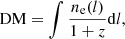
where n_e is the density of free electrons, l is the line-of-sight path, and z is the redshift.

Having well-localized (≲1″) FRBs with identified host galaxies allows us to study and understand the observed DM_FRB of a given FRB in terms of the contributions from different cosmological scales (Macquart et al. 2020). We can expand DM_FRB as

$$\begin{array}{c}\hfill {\mathrm{DM}}_{\mathrm{FRB}}={\mathrm{DM}}_{\mathrm{MW}}+{\mathrm{DM}}_{\mathrm{cosmic}}(z)+\frac{{\mathrm{DM}}_{\mathrm{host}}^{\mathrm{rest}}}{1+z},\end{array}$$(2)

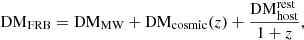
with

$$\begin{array}{c}\hfill {\mathrm{DM}}_{\mathrm{MW}}\equiv {\mathrm{DM}}_{\mathrm{MW}}^{\mathrm{ISM}}+{\mathrm{DM}}_{\mathrm{MW}}^{\mathrm{halo}},\end{array}$$(3)

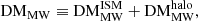
where DM${}_{\mathrm{MW}}^{\mathrm{ISM}}$ is the contribution from the Galactic interstellar medium (ISM), DM${}_{\mathrm{MW}}^{\mathrm{halo}}$ is the contribution from the Milky Way halo, DM${}_{\mathrm{host}}^{\mathrm{rest}}$ is the contribution from the host galaxy in its rest frame, including its halo, ISM, and any gas local to the event itself, and DM_cosmic(z) is the contribution from all other extragalactic gas, such as the ionized gas in the large-scale structure of the Universe and intervening halos of galaxies intersecting the FRB sightline (if any).

The ISM of the Milky Way is typically characterized using observations of the pulsar population, which is the basis of the NE2001 (Cordes & Lazio 2003) and YMW16 (Yao et al. 2017) Galactic electron density models. The average DM_cosmic component, ⟨DM_cosmic⟩, follows the Macquart relation (Macquart et al. 2020), which relates the redshift of the FRB host galaxy with the DM_cosmic(z).

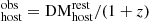
For the DM${}_{\mathrm{host}}^{\mathrm{rest}}$ contribution, it is common to use a fixed value (e.g., DM${}_{\mathrm{host},\mathrm{fix}}^{\mathrm{rest}}=50$ pc cm⁻³; Arcus et al. 2020, and references therein) or estimate it from a probability density function (PDF) expectation in the context of a Bayesian framework (typically log-normal; e.g., Macquart et al. 2020; James et al. 2022a,b; Khrykin et al. 2024b). Alternatively, other authors (e.g., Marcote et al. 2020; Niu et al. 2022; Lee et al. 2023) estimate it by rewriting Eq. (2) to solve for DM${}_{\mathrm{host}}^{\mathrm{rest}}$ (see Sect. 3.2). However, a single DM${}_{\mathrm{host}}^{\mathrm{rest}}$ value, or range (e.g., James et al. 2022b), for all FRB hosts (even at the same redshift) is not physically motivated because one expects local factors to directly affect the DM${}_{\mathrm{host}}^{\mathrm{rest}}$ value, such as the local density, clumpiness, and ionization state; similarly, the mass of the galaxy, the temperature of its halo, and the 3D position of the FRB source with respect to the observer must also affect the intrinsic DM_host value.

There are more direct estimations of DM_host¹ that explicitly attempt to take the contribution of the galaxy host ISM via nebular emission lines into account. For instance, Tendulkar et al. (2017) obtained an estimate of $55\le {\mathrm{DM}}_{\mathrm{host}}^{\mathrm{obs}}\le 225$ pc cm⁻³ at z = 0.19 based on Hα for FRB20121102A. Similarly, Chittidi et al. (2020) obtained DM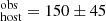${}_{\mathrm{host}}^{\mathrm{obs}}=150\pm 45$ pc cm⁻³ with the same method for the galaxy host of FRB20190608B at z = 0.117. Bannister et al. (2019) estimated $30\le {\mathrm{DM}}_{\mathrm{host}}^{\mathrm{obs}}\le 81$ pc cm⁻³ for the host galaxy of FRB20180924B at z = 0.32 using a Bayesian framework. In all these methods, the uncertainty on DM_host is large, and its value is difficult to determine precisely. It is therefore important to investigate whether there is a better way to determine the DM_host, which motivated this study.

Our goal is to obtain an empirical estimate for this DM_host component, referred to as DM${}_{\mathrm{host}}^{\mathrm{direct}}$, for a sample of several FRBs and analyzed in a homogeneous manner. In principle, to fully understand how the host galaxy affects DM_host, it is essential to consider not only the global properties of the galaxy but also the local environment of the FRB. The specific region from which the FRB originates can significantly influence the interpretation of observational data and the understanding of the physical mechanisms involved (Mannings et al. 2021; Woodland et al. 2024). To address this, in this work we explore if there is any difference in using nebular gas emission from the “global” ISM (full galaxy) or that “local” to the source (at the position of the FRB). Furthermore, we also investigated some possible relations between this DM${}_{\mathrm{host}}^{\mathrm{direct}}$ and internal properties of the host galaxies, such as stellar mass, the star formation rate (SFR), and the geometry between the FRB and the host galaxy (e.g., the projected distance of the FRB position and the galaxy center).

Our paper is structured as follows. In Sect. 2 we present the observational data and the sample analyzed in this study, including some key properties of the host galaxies. In Sect. 3 we elaborate on our direct method as well as a previous (indirect) method for estimating the DM_host. In Sect. 4 we report and discuss the results, while in Sect. 5 we provide a summary and our main conclusions. We assume a flat Λ cold dark matter cosmology with parameters consistent with the latest Planck 2018 measurements (Planck Collaboration VI 2020).

2. Data

2.1. Sample

We used a sample of 11 well-localized FRBs detected by the Commensal Real-Time ASKAP Fast-Transients (CRAFT) survey (Macquart et al. 2010) with identified host galaxies for which we have Very Large Telescope (VLT) Multi Unit Spectroscopic Explorer (MUSE) data (see below). We required better than 1″ precision for the FRB localization, and to make a confident host galaxy association we required a probabilistic association of transients to their hosts (PATH; Aggarwal et al. 2021) posterior probability greater than 90%. In addition to the CRAFT FRBs, we also included FRB20210410D, which was detected by the More TRAnsients and Pulsars (MeerTRAP; Rajwade et al. 2022) project and also satisfies the above criteria. Our final sample is composed of FRB host galaxies and is summarized in Table 1.

2.2. Previous observations

The Fast and Fortunate for FRB Follow-up (F⁴) is a collaboration endeavoring to obtain dedicated photometric and spectroscopic follow-up observations of localized FRBs and their host galaxies. All the observational data of our studied host galaxies except the Hα fluxes (e.g., stellar masses, SFRs, and FRB offsets) come from previous work done by F⁴ (see the last column of Table 1 for specific references) and are available on both the FRB GitHub repository² (Prochaska et al. 2023) and the “FRB Hosts” website³. We note that some values have been updated since their discovery papers, and here we used those reported by Gordon et al. (2023) and Shannon et al. (2024).

2.3. VLT/MUSE observations and data reduction

We wished to study the DM_host empirical contribution, and for this we used MUSE (Bacon et al. 2010), which is mounted on UT4 (Yepun) at the VLT on Cerro Paranal, Chile. MUSE provides resolved or partially resolved integral-field spectroscopy, which enables a “local” estimation of the ISM contribution to the host DM${}_{\mathrm{host}}^{\mathrm{ISM}}$ based on the Hα nebular emission at the FRB position (when available; see Sect. 3.1), and a “global” estimation based on the Hα nebular emission of the entire galaxy.

All the MUSE observations were conducted with the wide field mode with adaptive optics and nominal wavelength range mode. This setup provides a field of view of 1′×1′ with a spatial sampling of 0.2″ pix⁻¹, and spectral coverage of ≈4700 − 9300⁴ Å, with resolving power ranging from R ≃ 1770 at 4800 Å to R ≃ 3590 at 9300 Å. We observed each field for ∼4 − 8 × 600 s individual exposures with typical DIMM (Differential Image Motion Monitor) seeing conditions of ≈1″, which translated to ≲0.8″ point spread function thanks to the enabled AO. Table A.1 summarizes the dates, exposure times and program IDs of the observations.

Data reduction was performed using the ESO MUSE pipeline (v2.8.6, Weilbacher et al. 2020) within the ESO Recipe Execution Tool (EsoRex) environment (ESO CPL Development Team 2015). We used standard procedure and parameters.

3. Analysis

3.1. Direct DM_host estimation, DM${}_{\mathrm{host}}^{\mathrm{direct}}$

Here we provide a direct estimate of DM${}_{\mathrm{host}}^{\mathrm{direct}}$. For this estimation we consider two contributions, DM${}_{\mathrm{host}}^{\mathrm{ISM}}$ and DM${}_{\mathrm{host}}^{\mathrm{halo}}$, giving

$$\begin{array}{c}\hfill {\mathrm{DM}}_{\mathrm{host}}^{\mathrm{direct}}={\mathrm{DM}}_{\mathrm{host}}^{\mathrm{ISM}}+{\mathrm{DM}}_{\mathrm{host}}^{\mathrm{halo}},\end{array}$$(4)

where DM${}_{\mathrm{host}}^{\mathrm{ISM}}$ includes gas from the ISM of the galaxy host plus any possible gas associated with the FRB progenitor itself, while DM${}_{\mathrm{host}}^{\mathrm{halo}}$ is the contribution from the galactic halo, both defined in the source frame. The methodology to estimate these two contributions is presented as follows.

3.1.1. Estimating DM${}_{\mathrm{host}}^{\mathrm{ISM}}$

To estimate DM${}_{\mathrm{host}}^{\mathrm{ISM}}$ for the different galaxy hosts, we adopt the procedure outlined by Tendulkar et al. (2017) following Reynolds (1977). For completeness, we include the key equations here.

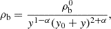
From the Hα flux measured by MUSE, we obtain the Hα surface brightness, S(Hα), by dividing the Hα line emission by the effective area considered. We correct the emission for the Galactic dust extinction (Fitzpatrick & Massa 2007) and by surface brightness dimming in order to pass from the observer’s frame to the source’s frame. From S(Hα), in the source’s frame, we use Eq. (10) of Reynolds (1977) to obtain an estimate of the emission measure (EM):

$$\begin{array}{c}\hfill \mathrm{EM}(\mathrm{H}\alpha )=2.75{\mathrm{pc}\mathrm{cm}}^{-6}{T}_4^{0.9}\left[\frac{S(\mathrm{H}\alpha )}{\mathrm{Rayleigh}}\right]·\end{array}$$(5)

Then, we adopted Eq. (5) from Tendulkar et al. (2017) to estimate DM${}_{\mathrm{host}}^{\mathrm{ISM}}$, in the source’s frame,

$$\begin{array}{c}\hfill {\mathrm{DM}}_{\mathrm{host}}^{\mathrm{ISM}}=387{\mathrm{pc}\mathrm{cm}}^{-3}{L}_{\mathrm{kpc}}^{1/2}{\left[\frac{f_{\mathrm{f}}}{\tau (1+{\zeta }^2)/4}\right]}^{1/2}{\left(\frac{\mathrm{EM}}{600{\mathrm{pc}\mathrm{cm}}^{-6}}\right)}^{1/2},\end{array}$$(6)

where f_f is the volume-filling factor of clouds, ζ represents the fractional density variation within any given cloud of ionized gas due to turbulence inside clouds, and τ is the density variation between any two clouds, all over a path length L_kpc in kpc (Cordes et al. 2016; Tendulkar et al. 2017; Chittidi et al. 2020).

Equation (6) was calibrated for the Milky Way and may not necessarily apply to FRB hosts in general. More fundamentally, even within the Milky Way, the clumpiness and density variations can vary significantly between sightlines and thus this estimation is inherently uncertain. Therefore, the exact values of the parameters governing DM${}_{\mathrm{host}}^{\mathrm{ISM}}$ are unknown. In what follows we assume a turbulent and dense environment in the sightline, that is, the volume-filling factor is at the maximum (f_f = 1) and that each ionized cloud along the sightline has internal density variations dominated by turbulence (ζ = 1) and that the variation between clouds is at the maximum (τ = 2). Finally, we assumed that the FRB comes from a path width similar to the Milky Way disk, that is, L_kpc = 0.15. In Sect. 4.5 we quantify the effect of these systematic uncertainties on our overall results.

3.1.2. Global and local DM${}_{\mathrm{host}}^{\mathrm{ISM}}$

To provide a global estimation for DM${}_{\mathrm{host}}^{\mathrm{ISM}}$, we used the Hα nebular emission within the area defined by an ellipse with the reported eccentricity and by using the galaxy’s effective radius as the semi-major axis, referred to as DM${}_{\mathrm{host}}^{\mathrm{ISM},\mathrm{global}}$. In addition, to have a more relevant DM${}_{\mathrm{host}}^{\mathrm{ISM}}$ estimation, we used the local nebular emission of Hα coincident with the FRB position, referred to as DM${}_{\mathrm{host}}^{\mathrm{ISM},\mathrm{local}}$. We obtained the local Hα emission from the MUSE datacubes by selecting a region of radius 0.4 arcsec (2 native spaxels), which corresponds to the typical seeing (comparable to or larger than the typical FRB positional uncertainty in our sample). Then, from this region we extracted the spectrum at the observed wavelengths corresponding to the Hα transition by summing the flux of all the spaxels with equal weight. We modeled the continuum as a spline, which is subtracted from the observed spectrum. Then we modeled the remaining emission line flux with a Gaussian fit. Figure 1 shows an example for FRB20191001A. The FRB localization is denoted by the blue circle. In the lower panel of the figure we show the extracted 1D spectrum within the region, at the wavelengths corresponding to the observed Hα emission, together with our modeled Gaussian fit and continuum. Finally, we integrated the Gaussian fit to obtain the total Hα nebular emission flux and its error. Table A.2 summarizes our results obtained for the global and local DM${}_{\mathrm{host}}^{\mathrm{ISM}}$ estimates.

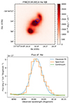Fig. 1. Hα emission at the FRB location. Upper: FRB20191001A host emission integrated at the narrow band encompassing Hα using the same wavelength range as shown in the bottom panel. The blue circle is centered at the FRB localization and has a radius of 0.4″, and the dashed black ellipse represents the actual FRB position uncertainty. Lower: Integrated spectrum of the Hα emission within the blue circle (orange). We fit this emission with a Gaussian (dashed blue) plus a continuum (green).

Uncertainties in these estimations are calculated as follows: We did 10⁵ realization of Hα, following a normal distribution around the calculate Hα for every FRB host, with the error of Hα as standard deviation. Then, with every realization we repeated the previous steps to provide an empirical 1σ uncertainty from the resulting PDF.

For the host galaxy of FRB20190711A at z = 0.522, the MUSE spectrum does not cover the redshifted Hα wavelength. In this case we followed a procedure similar to that used by Logroño-García et al. (2019), Calzetti et al. (2000) and Chittidi et al. (2020). We first obtained the Hβ flux and Hγ analogously. We then estimated the extinction from the observed ratio of Hγ to Hβ flux (0.397) and compared it to the theoretical value (0.466; Osterbrock & Ferland 2006). This gives us an extinction estimate of A_v = 0.18. With the extinction we could then calculate the intrinsic ratio of Hα to Hβ flux following Calzetti et al. (2000) and Logroño-García et al. (2019), obtaining 4.364. Finally, this ratio gives us our estimate of Hα (corrected for dust).

Given Eqs. (5) and (6), in addition to the geometrical factors and temperature, a key observable for inferring DM${}_{\mathrm{host}}^{\mathrm{ISM}}$ is the S(Hα). In our case we obtain S(Hα) for global (full galaxy) and local (at the FRB position) Hα, and a comparison between the two is shown in Fig. 2. We observe that the global measurement is systematically larger than the local one. The dark orange line shows the linear correlation between them, from which we infer a systematic difference of 19%, which translates to ≈14% in the inferred DM${}_{\mathrm{host}}^{\mathrm{ISM}}$ (see Eqs. 5 and 6).

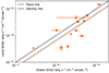Fig. 2. Comparison between the local and global inferred surface brightness of Hα, obtained from MUSE cubes, for our sample. The trend line (dark orange) has a slope of 1 by construction. The identity line (dashed line) corresponds to the 1:1 relation.

3.1.3. DM${}_{\mathrm{host}}^{\mathrm{halo}}$

To estimate the DM${}_{\mathrm{host}}^{\mathrm{halo}}$, we followed a procedure similar that in to Prochaska & Zheng (2019), Simha et al. (2023), and Chittidi et al. (2020). From the published estimated stellar mass for each host galaxy, we implemented the abundance matching technique to infer a halo mass (Moster et al. 2013). Then, following Prochaska & Zheng (2019), we estimated DM${}_{\mathrm{host}}^{\mathrm{halo}}$ assuming a density profile for the halo gas. We used the modified Navarro, Frenk, and White (mNFW) profile described by Prochaska & Zheng (2019) following Mathews & Prochaska (2017),

$$\begin{array}{c}\hfill {\rho }_{\mathrm{b}}=\frac{{\rho }_{\mathrm{b}}^0}{y^{1-\alpha }{(y_0+y)}^{2+\alpha }},\end{array}$$(7)

where y₀ = 2 and α = 2, y ≡ c(r/r₂₀₀), with c being the concentration parameter and r₂₀₀ is defined as the radius within which the average density is 200 times the critical density. Because we expect that not all of this gas is ionized, we needed to estimate the fraction of baryons that are ionized (f_hot). For this, we used f_hot = 55% (Khrykin et al. 2024a) as a fiducial value to calculate ρ_b⁰, which corresponds to the density of the ionized mass.

With ρ_b, we could calculate the density of free electrons, n_e, as

$$\begin{array}{c}\hfill n_{\mathrm{e}}={\mu }_{\mathrm{e}}\frac{{\rho }_{\mathrm{b}}}{m_{\mathrm{p}}{\mu }_{\mathrm{H}}},\end{array}$$(8)

with m_p the proton mass, μ_H = 1.3 the reduced mass (accounting for helium) and μ_e = 1.167 accounts for fully ionized helium and hydrogen. Corrections for heavy elements are negligible.

This profile is integrated along the line of sight, from the projected distance R of the FRB, to the max radius of the halo (r₂₀₀). The DM_halo(R) value is defined as

$$\begin{array}{c}\hfill {\mathrm{DM}}_{\mathrm{host}}^{\mathrm{halo}}(R)={\displaystyle \underset{0}{\overset{\sqrt{r_{200}^2-R^2}}{\int }}}{n}_{\mathrm{e}}\mathrm{d}s,\end{array}$$(9)

where the lower integration limit corresponds to the mid-plane of the halo, which is perpendicular to the line of sight. Finally, we evaluated Eq. (9) to obtain DM${}_{\mathrm{host}}^{\mathrm{halo}}$, in the source’s frame.

To account for uncertainties in DM${}_{\mathrm{host}}^{\mathrm{halo}}$ estimations derived from stellar mass for each host galaxy, we generated 1000 realizations of stellar masses, assuming a log-normal distribution where the standard deviation corresponds to the stellar mass uncertainty. For each stellar mass realization, we generated 100 additional realizations, varying the eight parameters of the Moster relation. The mean values and standard deviations for these parameters are taken from Table 1 of Moster et al. (2013), following a normal distribution. Finally, we obtained a PDF of DM${}_{\mathrm{host}}^{\mathrm{halo}}$ with 10⁵ realizations per FRB, and used the 1σ of this PDF as our final uncertainty. As an example, Fig. 3 shows this PDF for FRB20191001A.

Fig. 3. Distribution of DM${}_{\mathrm{host}}^{\mathrm{halo}}$ for FRB20191001A. The vertical solid black line represents the median value and the dashed black lines the corresponding 16th and 84th percentiles.

3.1.4. Estimating DM${}_{\mathrm{host}}^{\mathrm{direct}}$

To obtain DM${}_{\mathrm{host}}^{\mathrm{direct}}$, we added the two PDFs of DM${}_{\mathrm{host}}^{\mathrm{halo}}$ and DM${}_{\mathrm{host}}^{\mathrm{ISM}}$. From this sum, we generated a new PDF of DM${}_{\mathrm{host}}^{\mathrm{direct}}$ for each galaxy host in our sample; we used the median value as our DM${}_{\mathrm{host}}^{\mathrm{direct}}$ estimation and the 1σ as its uncertainties. For the calculation of DM${}_{\mathrm{host}}^{\mathrm{direct}}$ we used DM${}_{\mathrm{host}}^{\mathrm{ISM},\mathrm{local}}$. We note that in two cases (FRB20190611B and FRB20210117), the local Hα emission line was not detected (upper limits in Table A.2). However, these upper limits imply DM${}_{\mathrm{host}}^{\mathrm{ISM}}$ values comparable with those inferred from the global measurements (Fig. 2). Given that our systematic uncertainties in DM${}_{\mathrm{host}}^{\mathrm{ISM}}$ are much larger than these differences (see below), for simplicity in the following we treat these upper limits as actual measurements.

The systematic uncertainties of changing the values of the parameters in Eq. (6) are not taken into account for our reported values. For reference, they can make the DM${}_{\mathrm{host}}^{\mathrm{ISM}}$ up to two (three) times larger (smaller) than our fiducial values (see also Sect. 4.5). Similarly, the systematic uncertainty from the chosen path length, either in the ISM or in the halo, can make DM${}_{\mathrm{host}}^{\mathrm{ISM}}$/DM${}_{\mathrm{host}}^{\mathrm{halo}}$ up to 1.4 or 2 times larger, respectively, while in the case of the FRB being in the outskirts of the halo (unlikely given the known projected distance distributions), both these contributions could be as small as zero.

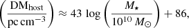
3.2. Estimating DM_host with the Macquart relation

For comparison, we also indirectly estimated the DM_host referred to as DM${}_{\mathrm{host}}^{\mathrm{Macquart}}$ (rest frame) using the follow equation:

$$\begin{array}{c}\hfill {\mathrm{DM}}_{\mathrm{host}}^{\mathrm{Macquart}}=(1+z)({\mathrm{DM}}_{\mathrm{FRB}}-{\mathrm{DM}}_{\mathrm{MW}}-⟨{\mathrm{DM}}_{\mathrm{cosmic}}⟩),\end{array}$$(10)

where ⟨DM_cosmic⟩ is the average contribution of extragalactic gas at redshift z. This analysis requires estimations of DM_MW and DM_cosmic.

3.2.1. DM_MW contribution

The Milky Way contribution comes from the ISM and the halo (Eq. 3). For DM${}_{\mathrm{MW}}^{\mathrm{ISM}}$, we used the NE2001 model (Cordes & Lazio 2003), where the free electrons are integrated across the Galaxy according to the FRB coordinates. NE2001 is a Galactic distribution model of free electrons that actually comprises two disk components: spiral arms, and localized regions (like the Magellanic Clouds). For DM${}_{\mathrm{MW}}^{\mathrm{halo}}$, we used a fixed value of 40 pc cm⁻³ (Prochaska & Zheng 2019).

3.2.2. DM${}_{\mathrm{host}}^{\mathrm{Macquart}}$ and upper limit on DM_host

Given our estimates of DM_MW for each FRB sightline, and ⟨DM_cosmic⟩ for an average sightline up to redshift z = z_frb (given by Λ cold dark matter), we used Eq. (10) to obtain the predicted Macquart DM_host, DM${}_{\mathrm{host}}^{\mathrm{Macquart}}$. We note that for two cases this DM${}_{\mathrm{host}}^{\mathrm{Macquart}}$ results in a negative (nonphysical) value; we nevertheless report them as such for the sake of completeness and for statistical consistency (see Sect. 4).

We caution the reader that every sightline is unique, and thus we expect deviations from ⟨DM_cosmic⟩ for individual FRBs with the majority of DM_cosmic expected to lie below this value (e.g., Baptista et al. 2024). This in turn implies that our DM${}_{\mathrm{host}}^{\mathrm{Macquart}}$ value will most of the time be an underestimation of the true DM_host, while the rest of the time an overestimation. However, we expect that the average DM${}_{\mathrm{host}}^{\mathrm{Macquart}}$ value of the ensemble of measurements to be close to the average true DM_host value of the ensemble, modulo systematic errors for example in DM_MW.

We used the same principle to estimate a maximum possible value of DM_host (rest frame), referred to as DM${}_{\mathrm{host}}^{\max }$, for a given individual FRB, following

$$\begin{array}{c}\hfill {\mathrm{DM}}_{\mathrm{host}}^{\max }=(1+z)({\mathrm{DM}}_{\mathrm{FRB}}-{\mathrm{DM}}_{\mathrm{MW}}^{\min }-{\mathrm{DM}}_{\mathrm{cosmic}}^{\min }),\end{array}$$(11)

where DM${}_{\mathrm{MW}}^{\min }$ is the minimum possible value for DM_MW allowed by the NE2001 model, and DM${}_{\mathrm{cosmic}}^{\min }$ being a conservative minimum contribution to DM_FRB by the intergalactic medium. For this, we used the lower 1% percentile of the allowed scatter around the Macquart relation, that is, assuming that the FRB traveled through an extremely under-dense sightline, without intersecting any dense cosmic web filament nor intervening halos of galaxies. Although it is very unlikely to observe such an extreme situation in a sample of only 12 FRBs, we used this estimation to provide a conservative upper limit for the DM_host.

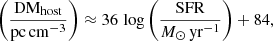
4. Results and discussion

Our DM${}_{\mathrm{host}}^{\mathrm{direct}}$ results are shown in Fig. 4 and summarized in Tables A.2 and A.3. We have found that, on average, ⟨DM_host⟩ = 80 ± 11 pc cm⁻³ with a standard deviation of the DM${}_{\mathrm{host}}^{\mathrm{direct}}$ distribution of 38 pc cm⁻³. This value is larger than the typically used value of 50 pc cm⁻³ (Arcus et al. 2020) but consistent within the uncertainties. In the following we investigate possible correlations of the individual DM${}_{\mathrm{host}}^{\mathrm{direct}}$ values as a function of galaxy properties including redshift, and also investigate the impact of possible systematic biases present in our current estimates.

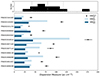Fig. 4. Estimates of DMhost for the 12 FRB hosts. The main panel shows each contribution of our empirical direct estimate (DM${}_{\mathrm{host}}^{\mathrm{direct}}$ in black points, DM${}_{\mathrm{host}}^{\mathrm{halo}}$ in dark blue and DM${}_{\mathrm{host}}^{\mathrm{ISM}}$ in light blue). The upper panel is the histogram for DM${}_{\mathrm{host}}^{\mathrm{direct}}$. The mean and the standard deviation (±1σ) of the distribution are represented by the vertical solid and dashed lines, respectively.

4.1. Comparison between DM${}_{\mathrm{host}}^{\mathrm{direct}}$ and DM${}_{\mathrm{host}}^{\mathrm{Macquart}}$

Figure 5 shows a comparison between our DM${}_{\mathrm{host}}^{\mathrm{direct}}$ measurements and the DM_host expectation from the Macquart relation, DM${}_{\mathrm{host}}^{\mathrm{Macquart}}$ (dark points). The figure also shows their corresponding average values of the ensemble (golden star): 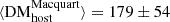$⟨{\mathrm{DM}}_{\mathrm{host}}^{\mathrm{Macquart}}⟩=179\pm 54$ pc cm⁻³, and $⟨{\mathrm{DM}}_{\mathrm{host}}^{\mathrm{direct}}⟩=80\pm 11$ pc cm⁻³, with the error bars being their corresponding standard deviations (186 and 31 pc cm⁻³, respectively).

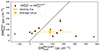Fig. 5. Relation between DM${}_{\mathrm{host}}^{\mathrm{direct}}$ and DM${}_{\mathrm{host}}^{\mathrm{Macquart}}$ (dark points), with error bars showing the statistical uncertainties on DM${}_{\mathrm{host}}^{\mathrm{direct}}$ (we did not estimate the uncertainties of our DM${}_{\mathrm{host}}^{\mathrm{Macquart}}$ values). The dashed line corresponds to the identity line (i.e., the 1:1 relation). The golden star corresponds to the average values of DM${}_{\mathrm{host}}^{\mathrm{direct}}$ and DM${}_{\mathrm{host}}^{\mathrm{Macquart}}$, with the error bars being their corresponding standard deviation.

Although individual measurements differ significantly between DM${}_{\mathrm{host}}^{\mathrm{direct}}$ and DM${}_{\mathrm{host}}^{\mathrm{Macquart}}$ (as expected), the average value is consistent between them, given their statistical uncertainties. We observe that 5 (7) out of 12 of our DM${}_{\mathrm{host}}^{\mathrm{direct}}$ measurements are larger (smaller) than their corresponding DM${}_{\mathrm{host}}^{\mathrm{Macquart}}$ values, implying that no obvious bias is present in our sample of FRBs and corresponding host galaxies for estimating the average DM${}_{\mathrm{host}}^{\mathrm{direct}}$ (see Sect. 3.2). Furthermore, we observe that the scatter in $⟨{\mathrm{DM}}_{\mathrm{host}}^{\mathrm{direct}}⟩$ is about ∼5 times smaller than the scatter in $⟨{\mathrm{DM}}_{\mathrm{host}}^{\mathrm{Macquart}}⟩$, which indicates that DM${}_{\mathrm{host}}^{\mathrm{direct}}$ may be a more precise measurement than DM${}_{\mathrm{host}}^{\mathrm{Macquart}}$; however, our empirical $⟨{\mathrm{DM}}_{\mathrm{host}}^{\mathrm{direct}}⟩$ estimate may be subject to systematic uncertainties (of order 30%; see Sect. 4.5) making it (in principle) less accurate than $⟨{\mathrm{DM}}_{\mathrm{host}}^{\mathrm{Macquart}}⟩$. Given that mostly cosmological parameters are involved in the estimation of DM${}_{\mathrm{host}}^{\mathrm{Macquart}}$, we only expect possible biases due to systematic errors in our individual DM_MW estimates or from the stochastic effect of foreground massive halos that could contribute to the observed DM (Lee et al. 2023). Although $⟨{\mathrm{DM}}_{\mathrm{host}}^{\mathrm{Macquart}}⟩$ may be more accurate it is nevertheless highly uncertain, but the fact that we find a consistency between $⟨{\mathrm{DM}}_{\mathrm{host}}^{\mathrm{direct}}⟩$ and $⟨{\mathrm{DM}}_{\mathrm{host}}^{\mathrm{Macquart}}⟩$ may indicate that systematic uncertainties are not dominating the measurements. Moreover, we computed the maximum possible DM${}_{\mathrm{host}}^{\max }$ based on our cosmological parameters (see Sect. 3.2), and all our DM${}_{\mathrm{host}}^{\mathrm{direct}}$ measurements are smaller than this limit (see Cols. 5 and 6 of Table A.3), ensuring consistency.

Finally, we note that we do not see any strong correlation between DM${}_{\mathrm{host}}^{\mathrm{direct}}$ and DM${}_{\mathrm{host}}^{\mathrm{Macquart}}$ (Pearson coefficient of −0.2, with a p-value of 0.6), which indicates that our current modeling could be missing an important DM contribution to the DM_FRB; in other words, some FRBs may have large intrinsic DM_host and/or a much larger actual DM_cosmic compared to the ⟨DM_cosmic⟩ (e.g., due to intervening foreground structures) that our modeling is not capturing or taken in consideration. The apparent lack of a correlation between the two estimates is partially driven by the two data points with the largest DM${}_{\mathrm{host}}^{\mathrm{Macquart}}$.

4.2. Correlations between DM${}_{\mathrm{host}}^{\mathrm{direct}}$ and galaxy properties

The left panel of Fig. 6 compares the DM${}_{\mathrm{host}}^{\mathrm{direct}}$ (black points) to the corresponding stellar masses of the host galaxies. We also show the individual contributions to the DM${}_{\mathrm{host}}^{\mathrm{direct}}$ from DM${}_{\mathrm{host}}^{\mathrm{halo}}$ (dark blue) and DM${}_{\mathrm{host}}^{\mathrm{ISM}}$ (light blue). We observe a positive correlation between DM${}_{\mathrm{host}}^{\mathrm{direct}}$ and stellar mass, of the form

$$\begin{array}{c}\hfill \left(\frac{{\mathrm{DM}}_{\mathrm{host}}}{{\mathrm{pc}\mathrm{cm}}^{-3}}\right)\approx 43log\left(\frac{M_{\star }}{{10}^{10}{M}_{\odot }}\right)+86,\end{array}$$(12)

with a Pearson correlation test giving a coefficient of 0.73 (with a p-value of 7 × 10⁻²). A correlation of DM_host with stellar mass is expected, given that the larger the stellar mass, the larger the halo mass used to estimate DM${}_{\mathrm{host}}^{\mathrm{halo}}$ (see Sect. 3.1.3). We also see a positive correlation between DM${}_{\mathrm{host}}^{\mathrm{halo}}$ and stellar mass with Pearson coefficient of 0.89 (with a p-value of 1 × 10⁻³). Interestingly, a positive correlation is also present between DM${}_{\mathrm{host}}^{\mathrm{ISM}}$ and stellar mass (Pearson coefficient of 0.64, with a p-value of 3 × 10⁻²), which we attribute to the fact that most galaxies in our sample are star-forming and the existence of the star formation main sequence (SFMS; e.g., Brinchmann et al. 2004; see below).

The middle panel of Fig. 6 shows DM${}_{\mathrm{host}}^{\mathrm{direct}}$ (black points) as a function of global SFR for each host galaxy; as before, the individual contributions of DM${}_{\mathrm{host}}^{\mathrm{halo}}$ (dark blue) and DM${}_{\mathrm{host}}^{\mathrm{ISM}}$ (light blue) are also shown. In this case we also observe a positive correlation between DM${}_{\mathrm{host}}^{\mathrm{direct}}$ (and its components) and global SFR of the form

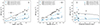Fig. 6. Rest-frame DM as a function of the stellar mass of the host (left), SFR of the host (middle), and projected offset from the center of the host (right). The black points correspond to DM${}_{\mathrm{host}}^{\mathrm{direct}}$, while the light blue and the dark blue points correspond to DM${}_{\mathrm{host}}^{\mathrm{ISM}}$ and DM${}_{\mathrm{host}}^{\mathrm{halo}}$, respectively. The black line shows a linear fit for DM${}_{\mathrm{host}}^{\mathrm{direct}}$ (=DM${}_{\mathrm{host}}^{\mathrm{halo}}$ + DM${}_{\mathrm{host}}^{\mathrm{ISM}}$), while the light blue and dark blue lines are the linear fits of DM${}_{\mathrm{host}}^{\mathrm{ISM}}$ and DM${}_{\mathrm{host}}^{\mathrm{halo}}$, respectively. The parameters of these fits are presented in Table B.1, and the Pearson coefficients and p-values are given in the figure legends.

$$\begin{array}{c}\hfill \left(\frac{{\mathrm{DM}}_{\mathrm{host}}}{{\mathrm{pc}\mathrm{cm}}^{-3}}\right)\approx 36log\left(\frac{\mathrm{SFR}}{M_{\odot }{\mathrm{yr}}^{-1}}\right)+84,\end{array}$$(13)

with a Pearson correlation test giving a coefficient of 0.85 (with a p-value of 4 × 10⁻³). A correlation with SFR could be expected given that galaxies with higher star formation activity should also have larger S(Hα), which is directly proportional to DM${}_{\mathrm{host}}^{\mathrm{ISM}}$ in our estimations (Eqs. 5 and 6). Despite the fact that we used local values of S(Hα) to estimate DM${}_{\mathrm{host}}^{\mathrm{ISM}}$, we have shown that for our sample the local and global values of S(Hα) are similar (see Fig. 2; see also Sect. 4.5). We also observe a positive correlation between DM${}_{\mathrm{host}}^{\mathrm{halo}}$ and the SFR (Pearson coefficient 0.91, with a p-value of 1 × 10⁻³), which can again be explained by the existence of the SFMS for star-forming galaxies.

To investigate whether the correlations between DM${}_{\mathrm{host}}^{\mathrm{ISM}}$ and stellar mass, and DM${}_{\mathrm{host}}^{\mathrm{halo}}$ and SFR are driven by the SFMS, we performed the following experiment. We used the nominal stellar mass values of the galaxies in our sample (without considering uncertainties) and obtained values for their SFR assuming they lie right on top of the SFMS fit reported by Chang et al. (2015) in their Eq. (4). From these, we obtained an expectation of the Hα flux using Eq. (14) from Pflamm-Altenburg et al. (2007), deriving an “expected” DM${}_{\mathrm{host}}^{\mathrm{ISM}}$ given the new S(Hα), and by following our methodology (Sect. 3.1.1) but for a global measurement rather than a local measurement (see also Sect. 3.1.2). We find a correlation between DM${}_{\mathrm{host}}^{\mathrm{ISM}}$ and DM${}_{\mathrm{host}}^{\mathrm{halo}}$ that is stronger than our actual case (using the actual local Hα measurements) and also stronger when we compare it with our actual global measurements. This indicates that the SFMS can indeed account for all the correlation observed between DM${}_{\mathrm{host}}^{\mathrm{ISM}}$ and DM${}_{\mathrm{host}}^{\mathrm{halo}}$, and hence both DM${}_{\mathrm{host}}^{\mathrm{ISM}}$ and stellar mass, and DM${}_{\mathrm{host}}^{\mathrm{halo}}$ and SFR.

Finally, we also explored a possible correlation between DM${}_{\mathrm{host}}^{\mathrm{direct}}$ and the projected distance of the FRB sightline with respect to the galaxy halo center. In the right panel of Fig. 6 we show DM${}_{\mathrm{host}}^{\mathrm{direct}}$ as a function of the projected distance of the FRB sightline to the center of their host galaxy (black points), again also showing their DM${}_{\mathrm{host}}^{\mathrm{halo}}$ (dark blue points) and DM${}_{\mathrm{host}}^{\mathrm{ISM}}$ (light blue points) contributions. In contrast to previous cases, we do not observe any strong correlation between DM${}_{\mathrm{host}}^{\mathrm{direct}}$ and FRB projected distances (we only report a weak anticorrelation), which can be explained by the fact that the most (least) massive galaxies have their FRBs farther (closer) to their centers. This result is driven by the adopted mNFW profiles, which produce a rather flat (weak anticorrelation) between DM${}_{\mathrm{host}}^{\mathrm{halo}}$ and projected distance (see Prochaska & Zheng 2019). Furthermore, the fact that FRBs tend to lie well within the center of the dark matter halos of their host galaxies indicate that the DM${}_{\mathrm{host}}^{\mathrm{halo}}$ is indeed dominated by the halo mass (i.e., stellar mass) rather than projected distance.

Table B.1 summarizes the parameters of our fits and correlation coefficients discussed in this section.

4.3. Possible redshift evolution of DM ${}_{\mathrm{host}}^{\mathrm{direct}}$ and redshift biases

We also investigated a possible redshift dependence in our DM_host estimates. Figure 7 shows DM_host as a function of redshift (top panel), where the black and red points correspond to DM${}_{\mathrm{host}}^{\mathrm{direct}}$ and DM${}_{\mathrm{host}}^{\mathrm{Macquart}}$, respectively. We observe no strong redshift evolution in the individual values of DM_host. The black line corresponds to a fit of the form

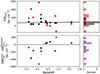Fig. 7. Dependency on Redshift. Top panel: DMhost as a function of redshift. Black and red points correspond to DM${}_{\mathrm{host}}^{\mathrm{direct}}$ and DM${}_{\mathrm{host}}^{\mathrm{Macquart}}$, respectively. The black line is the tendency of DM${}_{\mathrm{host}}^{\mathrm{direct}}$. Negative values for DM${}_{\mathrm{host}}^{\mathrm{Macquart}}$ are nonphysical; we nevertheless report them for statistical consistency. A histogram of the different samples is shown to the right following the same color scheme. Bottom panel: Difference between DM${}_{\mathrm{host}}^{\mathrm{direct}}$ and DM${}_{\mathrm{host}}^{\mathrm{Macquart}}$ as a function of redshift (purple dots). The dashed black line at value 0 indicates where DM${}_{\mathrm{host}}^{\mathrm{direct}}$ and DM${}_{\mathrm{host}}^{\mathrm{Macquart}}$ are equal. A histogram of the sample is shown in the right panel.

$$\begin{array}{c}\hfill {\mathrm{DM}}_{\mathrm{host}}^{\mathrm{direct}}(z)={\mathrm{DM}}_{\mathrm{host},0}{(1+z)}^{\alpha },\end{array}$$(14)

which shows a flat exponent (α ≈ 0.3 ± 1.7) and a DM_host, 0 ≈ 73 ± 33 pc cm⁻³, consistent with our $⟨{\mathrm{DM}}_{\mathrm{host}}^{\mathrm{direct}}⟩$. The apparent lack of redshift evolution indicates that DM_host is driven by internal galaxy properties (e.g., stellar mass and SFR) and thus no extra corrections for redshift (galaxy evolution) are needed, at least for z ≲ 0.5. We remind the reader that this DM_host estimate is in the rest frame, and thus a factor of (1 + z) should still be applied when considering DM${}_{\mathrm{host}}^{\mathrm{obs}}$ (see Eq. 2).

In contrast, the DM${}_{\mathrm{host}}^{\mathrm{Macquart}}$ estimations show a much larger scatter and a possible evolution with redshift, which may indicate a possible redshift bias. The bottom panel of Fig. 7 shows the difference between DM${}_{\mathrm{host}}^{\mathrm{direct}}$ and DM${}_{\mathrm{host}}^{\mathrm{Macquart}}$ as a function of redshift. Here, we also observe a possible bias as a function of redshift for individual measurements where DM${}_{\mathrm{host}}^{\mathrm{Macquart}}$ tend to be larger than our DM${}_{\mathrm{host}}^{\mathrm{direct}}$ at lower redshifts (z ≲ 0.3), and lower than DM${}_{\mathrm{host}}^{\mathrm{direct}}$ at higher redshifts (z ≳ 0.3). This discrepancy could be due to an underestimation of the Macquart relation at lower redshifts, making DM${}_{\mathrm{host}}^{\mathrm{Macquart}}$ systematically larger (see Eq. 11). Another possibility is that our calculation of DM${}_{\mathrm{host}}^{\mathrm{direct}}$ is underestimated at lower redshifts, caused by an unknown systematic effect; we note that the expected systematic error of ∼30% (see Sect. 4.5) is not enough to make this apparent redshift bias disappear. Given that our sample size is still small, there is also the possibility of this being driven by low number statistics (e.g., the current trend is partially induced by the two FRBs with the largest DM${}_{\mathrm{host}}^{\mathrm{Macquart}}$, which also correspond to the two largest values of DM_FRB), motivating future similar studies with larger samples.

4.4. Comparison with previous work

Our empirical estimation is consistent with recent observational results from Khrykin et al. (2024b) who reported $⟨{\mathrm{DM}}_{\mathrm{host}}⟩={90}_{-19}^{+29}$ pc cm⁻³ applied to a sample of eight FRB sightlines and using a different methodology. However, we note that six out of the eight were also included in our analysis, and thus these two results are not fully independent. Our empirical estimation is also consistent with that of Shin et al. (2023) who reported a median value of DM${}_{\mathrm{host}}={84}_{-49}^{+69}$ pc cm⁻³ for the FRBs detected by the Canadian Hydrogen Intensity Mapping Experiment (CHIME). In contrast, our results are inconsistent with those from Wang & van Leeuwen (2024), who reported much larger values, $⟨{\mathrm{DM}}_{\mathrm{host}}⟩={560}_{-190}^{+37}$ pc cm⁻³ for their power-law density model and $⟨{\mathrm{DM}}_{\mathrm{host}}⟩={490}_{-129}^{+74}$ pc cm⁻³ for their SFR model, as well as for CHIME FRBs. Our estimates are also lower than those reported by Bhardwaj et al. (2024) based on FRB scattering timescales, of ⟨DM_host⟩≳170 pc cm⁻³ for a range of galaxy inclinations.

In terms of recent theoretical work, Mo et al. (2023) analyzed cosmological hydrodynamical simulations using two different models for the location of FRBs within the simulated host galaxies: (i) following the star-formation, and (ii) following the stellar mass. They obtained different DM_host values for these different models, reporting medians of 179 and 63 pc cm⁻³ (rest frame), respectively. Our observational result lies between these two values, and is consistent with both of them given the reported uncertainties and large scatter across models. Mo et al. (2023) also report a linear relation between their inferred DM_host and the logarithm of the host stellar mass for both models following a similar trend as the one reported here, although again with much larger variations depending on the model used (see also Zhang et al. 2020; Kovacs et al. 2024). Finally, they report a possible evolution of DM_host (rest frame) with redshift using a power-law fit as we do here (Eq. 14), but with an α varying between 0.8 and 1.8 depending on the model (see also Zhang et al. 2020; Kovacs et al. 2024; Orr et al. 2024), whereas we do not see any evolution from our current sample (see Sect. 4.3). Therefore, empirical DM_host estimations have the potential to constrain sub-grid physics of galaxy evolution (e.g., Khrykin et al. 2024b) and also provide important clues for the origin of FRBs themselves.

4.5. Systematic uncertainties

In this work we modeled DM${}_{\mathrm{host}}^{\mathrm{direct}}$ as the sum of two contributions: DM${}_{\mathrm{host}}^{\mathrm{ISM}}$ and DM${}_{\mathrm{host}}^{\mathrm{halo}}$ (see Sect. 3.1). Out of these two estimates, we consider that DM${}_{\mathrm{host}}^{\mathrm{ISM}}$ is more uncertain than DM${}_{\mathrm{host}}^{\mathrm{halo}}$ because of the several assumptions regarding geometry, temperature, and other properties of the ISM, and such systematic effects are not fully accounted for in our reported statistical uncertainties; for instance, recent studies of pulsars in the Large Magellanic Cloud report variations of observed DMs of several tens of pc cm⁻³ (e.g., Prayag et al. 2024, see their Table 1). In a more extreme situation, if FRBs originate outside the disks of galaxies (e.g., globular clusters; Kirsten et al. 2022), then DM${}_{\mathrm{host}}^{\mathrm{ISM}}\sim 0$ pc cm⁻³, at least for those cases in which the FRB is foreground to the disk itself. Although the DM${}_{\mathrm{host}}^{\mathrm{halo}}$ inferences also depend on several systematic factors, including the assumed model of baryons around galaxies (Eq. 9), ionization fraction (f_hot) and the path length of the FRB along the galaxy host halo, the fact that we sampled DM${}_{\mathrm{host}}^{\mathrm{halo}}$ from a PDF that does include (already large) uncertainties in both the stellar mass and the dark matter halo mass, makes their systematic effect less important relative to those associated with DM${}_{\mathrm{host}}^{\mathrm{ISM}}$.

To estimate such a systematic effect, we repeated our individual DM${}_{\mathrm{host}}^{\mathrm{direct}}$ measurements using 10⁵ realizations of DM${}_{\mathrm{host}}^{\mathrm{ISM}}$ uniformly sampled from a PDF whose mean value is between [0.5] and [1.5] times our fiducial values (e.g., those reported in Table A.2, Col. 6), leaving DM${}_{\mathrm{host}}^{\mathrm{halo}}$ unchanged (see Sect. 3.1.4 and Eq. 4). We consider that such a range in variation includes most of the systematic uncertainties in DM${}_{\mathrm{host}}^{\mathrm{ISM}}$ (including geometrical factors that appear in Eq. 6). Figure C.1 shows the effect of this experiment in our DM${}_{\mathrm{host}}^{\mathrm{direct}}$ measurement, where the shaded orange region represents the 1σ uncertainty (systematic) around our fiducial trends, corresponding to a ∼30% (systematic) impact on DM${}_{\mathrm{host}}^{\mathrm{direct}}$.

In the context of measuring DM${}_{\mathrm{host}}^{\mathrm{ISM}}$, one can consider either a global or a local measurement of S(Hα) (see Sect. 3.1.2). In our sample we have empirically found that the two give similar results (see Fig. 2) if we take their statistical uncertainties into account. Such a result is partly driven by some of our galaxies not being fully resolved (7 out of the 12 have half-light radii comparable with the 0.4″ radius used for our local measurement). Similarly, we find that the larger differences between the two are coming from FRBs that have larger projected distances with respect to the disks traced by Hα (as expected), but these cases are a minority (namely FRB20190611B and FRB20210117A). In other words, most of the FRBs in our sample are coming from galaxy disks (e.g., Mannings et al. 2021). The systematic difference between the two is small and only implies a ≈14% bias in DM${}_{\mathrm{host}}^{\mathrm{ISM}}$, which is already contained in the ∼30% systematic uncertainty budget reported above. Therefore, we conclude that estimating DM${}_{\mathrm{host}}^{\mathrm{ISM}}$ from a global Hα measurement provides similar level of accuracy than using a local estimate for partially resolved galaxies. This is not to say that the two are the same; it is just an observational limitation of our adopted technique. Finally, considering a more extreme (yet unlikely) situation where DM${}_{\mathrm{host}}^{\mathrm{ISM}}=0$ pc cm⁻³, then only our results for DM${}_{\mathrm{host}}^{\mathrm{halo}}$ (e.g., see Table B.1) should be used as reference for DM${}_{\mathrm{host}}^{\mathrm{direct}}$ instead.

5. Summary and conclusions

In this work we empirically estimated the DM of FRB host galaxies, DM_host, using a sample of 12 well-localized FRBs at redshifts 0.11 < z < 0.53 observed with VLT/MUSE. For this estimation, we employed a method that uses the stellar mass of the host galaxies and the projected distance to the FRBs to infer the contribution from the host halos (DM${}_{\mathrm{host}}^{\mathrm{halo}}$) and uses the Hα nebular emission line flux to infer the contribution from their ISM (DM${}_{\mathrm{host}}^{\mathrm{ISM}}$). The sum of these two contributions is our direct estimation of DM_host, which we call the DM${}_{\mathrm{host}}^{\mathrm{direct}}$ (see Eq. 4). For comparison purposes we also estimated the inferred DM_host, assuming that the sightlines to the FRBs have an intergalactic medium DM contribution given by the Macquart relation, referred to as DM${}_{\mathrm{host}}^{\mathrm{Macquart}}$ (see Eq. 10). We summarize our main results as follows:

1. We find that, on average, ⟨DM_host⟩ = 80 ± 11 pc cm⁻³ with a standard deviation of 38 pc cm⁻³ (the uncertainty here is only statistical). We have estimated a systematic uncertainty of ∼30% for our results, which is mostly due to the unknown physical properties of the host ISM gas through which the FRB pulse propagated (including the immediate environment around the progenitor). Our reported DM${}_{\mathrm{host}}^{\mathrm{direct}}$ is larger than the typically used (fixed) value of 50 pc cm⁻³ but consistent within the uncertainties.

2. We find no strong correlation between DM${}_{\mathrm{host}}^{\mathrm{direct}}$ and DM${}_{\mathrm{host}}^{\mathrm{Macquart}}$, indicating that our current modeling could be missing an important DM contribution to the DM_FRB for a fraction of FRBs (e.g., intrinsic variations to DM_host and/or unaccounted for intervening halos or cosmic web structures).

3. We find a positive correlation between DM${}_{\mathrm{host}}^{\mathrm{direct}}$ with the stellar mass and SFR of the host galaxy (see Fig. 6) of the form given by Eqs. (12) and (13) (parameters summarized in Table B.1). In contrast, no strong correlation is observed between DM${}_{\mathrm{host}}^{\mathrm{direct}}$ and the FRB projected distance with respect to the host centers (see Sect. 4.2).

4. We do not find any strong redshift evolution of DM_host (rest frame) in our sample (Fig. 7 and Sect. 4.3). However, we find a possible redshift bias associated with the indirect estimation of DM_host based on the Macquart relation and/or produced by an unknown bias in our DM${}_{\mathrm{host}}^{\mathrm{direct}}$ measurements.

Our reported correlations and the lack of a strong redshift evolution can be used to constrain models for the progenitor of FRBs, for example by comparing them with theoretical models. However, larger samples are needed to improve upon the present results and thus provide more precise and accurate observed values of DM_host.

Data availability

An external appendix is available on Zenodo at https://zenodo.org/records/14745235. This appendix provides, as in Fig. 1, the location of the FRB within the host galaxy, along with the corresponding extracted spectrum for the sample. The galaxy map corresponds to the measured emission line (Hα, Hβ, or Hγ, as appropriate).

Acknowledgments

We thank the anonymous referee for their careful revision and suggestions that improved the paper. We thank Ron Ekers and Kasper Heintz for useful comments and discussions. This work is based on observations collected at the European Southern Observatory under ESO programmes 2102.A-5005, 0104.A-0411, 0105.20HG and 0110.241Y. LBC and NT acknowledge support by FONDECYT grant 11191217. LBC acknowledge support by Beca Postgrado PUCV 2022-2023. ISK and NT acknowledge the support received by the Joint Committee ESO-Government of Chile grant ORP 40/2022. LBC, NT, ISK, and JXP, as members of the Fast and Fortunate for FRB Follow-up team, acknowledge support from NSF grants AST-1911140, AST-1910471 and AST-2206490. LM is supported by an Australian Government Research Training Program (RTP) Scholarship. RMS acknowledges support through Australian Research Council Future Fellowship FT190100155 and Discovery Project DP220102305.

References

Appendix A: Tables

This appendix provides the supplementary tables that complement the main article.

Appendix B: Parameters of the reported fits

In Table B.1 we present a summary of the parameters reported in our fits of Sect. 4.2.

Appendix C: Systematic uncertainty estimation of our reported trends

In Fig. C.1 we show our estimated systematic uncertainties (shaded brown regions) for the different reported trends of Sect. 4.2. Details on how this is done are given in in Sect. 4.5.

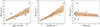Fig. C.1. DM${}_{\mathrm{host}}^{\mathrm{direct}}$ vs. stellar mass (in log scale; left), SFR (in log scale; middle), and projected distance (right) of the host galaxies. The black points and the black lines are the same as those in Fig. 6. The shaded area corresponds to our estimated systematic uncertainty (see Sect. 4.5).

All Tables

All Figures

Fig. 1. Hα emission at the FRB location. Upper: FRB20191001A host emission integrated at the narrow band encompassing Hα using the same wavelength range as shown in the bottom panel. The blue circle is centered at the FRB localization and has a radius of 0.4″, and the dashed black ellipse represents the actual FRB position uncertainty. Lower: Integrated spectrum of the Hα emission within the blue circle (orange). We fit this emission with a Gaussian (dashed blue) plus a continuum (green).

In the text

	Fig. 2. Comparison between the local and global inferred surface brightness of Hα, obtained from MUSE cubes, for our sample. The trend line (dark orange) has a slope of 1 by construction. The identity line (dashed line) corresponds to the 1:1 relation.
In the text

	Fig. 3. Distribution of DM${}_{\mathrm{host}}^{\mathrm{halo}}$ for FRB20191001A. The vertical solid black line represents the median value and the dashed black lines the corresponding 16th and 84th percentiles.
In the text

Fig. 4. Estimates of DMhost for the 12 FRB hosts. The main panel shows each contribution of our empirical direct estimate (DM${}_{\mathrm{host}}^{\mathrm{direct}}$ in black points, DM${}_{\mathrm{host}}^{\mathrm{halo}}$ in dark blue and DM${}_{\mathrm{host}}^{\mathrm{ISM}}$ in light blue). The upper panel is the histogram for DM${}_{\mathrm{host}}^{\mathrm{direct}}$. The mean and the standard deviation (±1σ) of the distribution are represented by the vertical solid and dashed lines, respectively.

In the text

Fig. 5. Relation between DM${}_{\mathrm{host}}^{\mathrm{direct}}$ and DM${}_{\mathrm{host}}^{\mathrm{Macquart}}$ (dark points), with error bars showing the statistical uncertainties on DM${}_{\mathrm{host}}^{\mathrm{direct}}$ (we did not estimate the uncertainties of our DM${}_{\mathrm{host}}^{\mathrm{Macquart}}$ values). The dashed line corresponds to the identity line (i.e., the 1:1 relation). The golden star corresponds to the average values of DM${}_{\mathrm{host}}^{\mathrm{direct}}$ and DM${}_{\mathrm{host}}^{\mathrm{Macquart}}$, with the error bars being their corresponding standard deviation.

In the text

Fig. 6. Rest-frame DM as a function of the stellar mass of the host (left), SFR of the host (middle), and projected offset from the center of the host (right). The black points correspond to DM${}_{\mathrm{host}}^{\mathrm{direct}}$, while the light blue and the dark blue points correspond to DM${}_{\mathrm{host}}^{\mathrm{ISM}}$ and DM${}_{\mathrm{host}}^{\mathrm{halo}}$, respectively. The black line shows a linear fit for DM${}_{\mathrm{host}}^{\mathrm{direct}}$ (=DM${}_{\mathrm{host}}^{\mathrm{halo}}$ + DM${}_{\mathrm{host}}^{\mathrm{ISM}}$), while the light blue and dark blue lines are the linear fits of DM${}_{\mathrm{host}}^{\mathrm{ISM}}$ and DM${}_{\mathrm{host}}^{\mathrm{halo}}$, respectively. The parameters of these fits are presented in Table B.1, and the Pearson coefficients and p-values are given in the figure legends.

In the text

Fig. 7. Dependency on Redshift. Top panel: DMhost as a function of redshift. Black and red points correspond to DM${}_{\mathrm{host}}^{\mathrm{direct}}$ and DM${}_{\mathrm{host}}^{\mathrm{Macquart}}$, respectively. The black line is the tendency of DM${}_{\mathrm{host}}^{\mathrm{direct}}$. Negative values for DM${}_{\mathrm{host}}^{\mathrm{Macquart}}$ are nonphysical; we nevertheless report them for statistical consistency. A histogram of the different samples is shown to the right following the same color scheme. Bottom panel: Difference between DM${}_{\mathrm{host}}^{\mathrm{direct}}$ and DM${}_{\mathrm{host}}^{\mathrm{Macquart}}$ as a function of redshift (purple dots). The dashed black line at value 0 indicates where DM${}_{\mathrm{host}}^{\mathrm{direct}}$ and DM${}_{\mathrm{host}}^{\mathrm{Macquart}}$ are equal. A histogram of the sample is shown in the right panel.

In the text

	Fig. C.1. DM${}_{\mathrm{host}}^{\mathrm{direct}}$ vs. stellar mass (in log scale; left), SFR (in log scale; middle), and projected distance (right) of the host galaxies. The black points and the black lines are the same as those in Fig. 6. The shaded area corresponds to our estimated systematic uncertainty (see Sect. 4.5).
In the text

References

- Aggarwal, K., Budavári, T., Deller, A. T., et al. 2021, ApJ, 911, 95 [NASA ADS] [CrossRef] [Google Scholar]
- Arcus, W. R., Macquart, J. P., Sammons, M. W., James, C. W., & Ekers, R. D. 2020, MNRAS, 501, 5319 [Google Scholar]
- Bacon, R., Accardo, M., Adjali, L., et al. 2010, Proc. SPIE, 7735, 773508 [Google Scholar]
- Bannister, K. W., Deller, A. T., Phillips, C., et al. 2019, Science, 365, 565 [NASA ADS] [CrossRef] [Google Scholar]
- Baptista, J., Prochaska, J. X., Mannings, A. G., et al. 2024, ApJ, 965, 57 [Google Scholar]
- Bhandari, S., Bannister, K. W., Lenc, E., et al. 2020, ApJ, 901, L20 [NASA ADS] [CrossRef] [Google Scholar]
- Bhandari, S., Heintz, K. E., Aggarwal, K., et al. 2022, AJ, 163, 69 [NASA ADS] [CrossRef] [Google Scholar]
- Bhandari, S., Gordon, A. C., Scott, D. R., et al. 2023, ApJ, 948, 67 [NASA ADS] [CrossRef] [Google Scholar]
- Bhardwaj, M., Lee, J., & Ji, K. 2024, Nature, 634, 1065 [Google Scholar]
- Brinchmann, J., Charlot, S., White, S. D. M., et al. 2004, MNRAS, 351, 1151 [Google Scholar]
- Caleb, M., Driessen, L. N., Gordon, A. C., et al. 2023, MNRAS, 524, 2064 [NASA ADS] [CrossRef] [Google Scholar]
- Calzetti, D., Armus, L., Bohlin, R. C., et al. 2000, ApJ, 533, 682 [NASA ADS] [CrossRef] [Google Scholar]
- Chang, Y.-Y., van der Wel, A., da Cunha, E., & Rix, H.-W. 2015, ApJS, 219, 8 [Google Scholar]
- Chittidi, J. S., Simha, S., Mannings, A., et al. 2020, ApJ, 922, 173 [Google Scholar]
- Cordes, J. M., & Chatterjee, S. 2019, ARA&A, 57, 417 [NASA ADS] [CrossRef] [Google Scholar]
- Cordes, J. M., & Lazio, T. J. W. 2003, ArXiv e-prints [arXiv:astro-ph/0301598] [Google Scholar]
- Cordes, J. M., Wharton, R. S., Spitler, L. G., Chatterjee, S., & Wasserman, I. 2016, ArXiv e-prints [arXiv:1605.05890] [Google Scholar]
- Dall’Osso, S., La Placa, R., Stella, L., Bakala, P., & Possenti, A. 2024, ApJ, 973, 123 [Google Scholar]
- Day, C. K., Deller, A. T., Shannon, R. M., et al. 2020, MNRAS, 497, 3335 [NASA ADS] [CrossRef] [Google Scholar]
- ESO CPL Development Team 2015, Astrophysics Source Code Library [record ascl:1504.003] [Google Scholar]
- Fitzpatrick, E. L., & Massa, D. 2007, ApJ, 663, 320 [Google Scholar]
- Gordon, A. C., Fong, W.-F., Kilpatrick, C. D., et al. 2023, ApJ, 954, 80 [NASA ADS] [CrossRef] [Google Scholar]
- Heintz, K. E., Xavier Prochaska, J., Simha, S., et al. 2020, ApJ, 903, 152 [NASA ADS] [CrossRef] [Google Scholar]
- James, C. W., Ghosh, E. M., Prochaska, J. X., et al. 2022a, MNRAS, 516, 4862 [NASA ADS] [CrossRef] [Google Scholar]
- James, C. W., Prochaska, J. X., Macquart, J. P., et al. 2022b, MNRAS, 509, 4775 [Google Scholar]
- Khrykin, I. S., Sorini, D., Lee, K.-G., & Davé, R. 2024a, MNRAS, 529, 537 [NASA ADS] [CrossRef] [Google Scholar]
- Khrykin, I. S., Ata, M., Lee, K.-G., et al. 2024b, ApJ, 973, 151 [Google Scholar]
- Kirsten, F., Marcote, B., Nimmo, K., et al. 2022, Nature, 602, 585 [NASA ADS] [CrossRef] [Google Scholar]
- Kovacs, T. O., Mao, S. A., Basu, A., et al. 2024, A&A, 690, A47 [NASA ADS] [CrossRef] [EDP Sciences] [Google Scholar]
- Lee, K.-G., Khrykin, I. S., Simha, S., et al. 2023, ApJ, 954, L7 [NASA ADS] [CrossRef] [Google Scholar]
- Logroño-García, R., Vilella-Rojo, G., López-Sanjuan, C., et al. 2019, A&A, 622, A180 [Google Scholar]
- Lorimer, D. R., Bailes, M., McLaughlin, M. A., Narkevic, D. J., & Crawford, F. 2007, Science, 318, 777 [Google Scholar]
- Macquart, J.-P., Bailes, M., Bhat, N. D. R., et al. 2010, PASA, 27, 272 [NASA ADS] [CrossRef] [Google Scholar]
- Macquart, J. P., Prochaska, J. X., McQuinn, M., et al. 2020, Nature, 581, 391 [Google Scholar]
- Mannings, A. G., Fong, W.-F., Simha, S., et al. 2021, ApJ, 917, 75 [NASA ADS] [CrossRef] [Google Scholar]
- Marcote, B., Nimmo, K., Hessels, J. W., et al. 2020, Nature, 577, 190 [NASA ADS] [CrossRef] [Google Scholar]
- Mathews, W. G., & Prochaska, J. X. 2017, ApJ, 846, L24 [Google Scholar]
- Michilli, D., Seymour, A., Hessels, J. W. T., et al. 2018, Nature, 553, 182 [Google Scholar]
- Mo, J.-F., Zhu, W., Wang, Y., Tang, L., & Feng, L.-L. 2023, MNRAS, 518, 539 [Google Scholar]
- Moster, B. P., Naab, T., & White, S. D. 2013, MNRAS, 428, 3121 [Google Scholar]
- Niu, C. H., Aggarwal, K., Li, D., et al. 2022, Nature, 606, 873 [NASA ADS] [CrossRef] [Google Scholar]
- Orr, M. E., Burkhart, B., Lu, W., Ponnada, S. B., & Hummels, C. B. 2024, ApJ, 972, L26 [Google Scholar]
- Osterbrock, D. E., & Ferland, G. J. 2006, Astrophysics of Gaseous Nebulae and Active Galactic Nuclei (Sausalito: University Science Books) [Google Scholar]
- Ouyed, R., Leahy, D., & Koning, N. 2020, RAA, 20, 027 [Google Scholar]
- Petroff, E., Hessels, J. W. T., & Lorimer, D. R. 2019, A&ARv, 27, 4 [NASA ADS] [CrossRef] [Google Scholar]
- Petroff, E., Hessels, J. W. T., & Lorimer, D. R. 2022, A&ARv, 30, 2 [NASA ADS] [CrossRef] [Google Scholar]
- Pflamm-Altenburg, J., Weidner, C., & Kroupa, P. 2007, ApJ, 671, 1550 [NASA ADS] [CrossRef] [Google Scholar]
- Planck Collaboration VI. 2020, A&A, 641, A6 [NASA ADS] [CrossRef] [EDP Sciences] [Google Scholar]
- Platts, E., Weltman, A., Walters, A., et al. 2019, Phys. Rep., 821, 1 [NASA ADS] [CrossRef] [Google Scholar]
- Prayag, V., Levin, L., Geyer, M., et al. 2024, MNRAS, 533, 2570 [NASA ADS] [CrossRef] [Google Scholar]
- Prochaska, J. X., & Zheng, Y. 2019, MNRAS, 485, 648 [NASA ADS] [Google Scholar]
- Prochaska, J. X., Simha, S., Almannin, et al. 2023, https://doi.org/10.5281/zenodo.8125230 [Google Scholar]
- Rajwade, K. M., Bezuidenhout, M. C., Caleb, M., et al. 2022, MNRAS, 514, 1961 [Google Scholar]
- Reynolds, R. J. 1977, ApJ, 216, 433 [NASA ADS] [CrossRef] [Google Scholar]
- Shannon, R. M., Bannister, K. W., Bera, A., et al. 2024, ArXiv e-prints [arXiv:2408.02083] [Google Scholar]
- Shin, K., Masui, K. W., Bhardwaj, M., et al. 2023, ApJ, 944, 105 [NASA ADS] [CrossRef] [Google Scholar]
- Simha, S., Lee, K.-G., Prochaska, J. X., et al. 2023, ApJ, 954, 71 [NASA ADS] [CrossRef] [Google Scholar]
- Tendulkar, S. P., Bassa, C. G., Cordes, J. M., et al. 2017, ApJ, 834, L7 [NASA ADS] [CrossRef] [Google Scholar]
- Wang, Y., & van Leeuwen, J. 2024, A&A, 690, A377 [NASA ADS] [CrossRef] [EDP Sciences] [Google Scholar]
- Weilbacher, P. M., Palsa, R., Streicher, O., et al. 2020, A&A, 641, A28 [NASA ADS] [CrossRef] [EDP Sciences] [Google Scholar]
- Woodland, M., Mannings, A., Prochaska, J., et al. 2024, Am. Astron. Soc. Meet. Abstr., 243, 359.07 [Google Scholar]
- Yao, J. M., Manchester, R. N., & Wang, N. 2017, ApJ, 835, 29 [NASA ADS] [CrossRef] [Google Scholar]
- Zhang, G. Q., Yu, H., He, J. H., & Wang, F. Y. 2020, ApJ, 900, 170 [NASA ADS] [CrossRef] [Google Scholar]