| Issue |
A&A
Volume 690, October 2024
|
|
|---|---|---|
| Article Number | A377 | |
| Number of page(s) | 20 | |
| Section | Extragalactic astronomy | |
| DOI | https://doi.org/10.1051/0004-6361/202450673 | |
| Published online | 22 October 2024 | |
Birth and evolution of fast radio bursts: Strong population-based evidence for a neutron-star origin
1
Anton Pannekoek Institute for Astronomy, University of Amsterdam, Science Park 904, 1098 XH Amsterdam, The Netherlands
2
ASTRON, the Netherlands Institute for Radio Astronomy, Oude Hoogeveensedijk 4, 7991 PD Dwingeloo, The Netherlands
Received:
9
May
2024
Accepted:
23
July
2024
Abstract
While the appeal of their extraordinary radio luminosity to our curiosity is undiminished, the nature of fast radio bursts (FRBs) has remained unclear. The challenge has been due in part to small sample sizes and limited understanding of telescope selection effects. We here present the first inclusion of the entire set of one-off FRBs from CHIME/FRB Catalog 1 in frbpoppy. Where previous work had to curate this data set, and fit for few model parameters, we have developed full multi-dimensional Markov chain Monte Carlo (MCMC) capabilities for frbpoppy – the comprehensive, open-science FRB population synthesis code – that allow us to include all one-off CHIME bursts. Through the combination of these two advances we now find the best description of the real, underlying FRB population, with higher confidence than before. We show that 4 ± 3 × 10³ one-off FRBs go off every second between Earth and z = 1; and we provide a mock catalog based on our best model, for straightforward inclusion in other studies. We investigate CHIME side-lobe detection fractions, and FRB luminosity characteristics, to show that some bright, local FRBs are still being missed. We find strong evidence that FRB birth rates evolve with the star formation rate of the Universe, even with a hint of a short (0.1−1 Gyr) delay time. The preferred contribution of the hosts to the FRB dispersion agrees with a progenitor birth location in the host disk. This population-based evidence solidly aligns with magnetar-like burst sources, and we conclude FRBs are emitted by neutron stars.
Key words: relativistic processes / methods: statistical / stars: magnetars / stars: neutron / radio continuum: general
Corresponding authors; This email address is being protected from spambots. You need JavaScript enabled to view it. , This email address is being protected from spambots. You need JavaScript enabled to view it.
© The Authors 2024
 Open Access article, published by EDP Sciences, under the terms of the Creative Commons Attribution License (https://creativecommons.org/licenses/by/4.0), which permits unrestricted use, distribution, and reproduction in any medium, provided the original work is properly cited.
This article is published in open access under the Subscribe to Open model. This email address is being protected from spambots. You need JavaScript enabled to view it. to support open access publication.
1. Introduction
Fast radio bursts (FRBs) are millisecond-duration phenomena visible in the radio band. Their origin is extragalactic, implying very high energies are involved (see, e.g., Cordes & Chatterjee 2019; Petroff et al. 2019, 2022, for reviews). After a first specimen was discovered in 2007 using single-pulse searches of archival Parkes telescope data (Lorimer et al. 2007), the bursts were not proven beyond a doubt as an astrophysical phenomenon (see Burke-Spolaor et al. 2010; Petroff et al. 2015, for similar human-generated signals) until four more events were found in the next decade (Thornton et al. 2013). However, their physical origins are still unclear after a further decade of studies. In general, FRBs are now empirically divided into two categories, one-offs and repeaters, depending on whether the burst is observed to recur or not. However, whether these two populations are intrinsically or physically different is still an open question. Furthermore, the periodic activity in some repeaters and host galaxy localizations for both classes are interesting for investigating their nature (see Petroff et al. 2022, and references therein), while their use for studying the intergalactic medium is also promising (e.g., Pastor-Marazuela et al. 2021).
In the early days of FRB discovery, opportunities for more quantitative studies of the FRB population were limited. This is changing: since the Canadian Hydrogen Intensity Mapping Experiment (CHIME/FRB; CHIME/FRB Collaboration 2019) finds 13 FRBs during its pre-commissioning runs, the ability to detect 𝒪(1) to 𝒪(10) FRBs per sky per day has made statistical studies of the FRB population feasible. The more than 500 FRBs contained in CHIME/FRB Catalog 1 (CHIME/FRB Collaboration 2021) have been the subject of several initial population studies (e.g., Chawla et al. 2022; Shin et al. 2023; Bhattacharyya et al. 2023).
Population synthesis provides a method to study the intrinsic properties of an astronomical class, by treating the various observational biases encountered, which are hard to remove analytically. Such studies have previously been carried out in a field akin to FRBs, for understanding neutron stars (e.g., Taylor & Manchester 1977; van Leeuwen & Stappers 2010; Bates et al. 2014). In FRB detection and interpretation, coupling between the intrinsic characteristics of the sources and of the detecting instrument introduces similar, possibly strong biases (see, e.g., Connor 2019). frbpoppy1 is an open source python package for population synthesis of FRBs (Gardenier 2019). It simulates the intrinsic, cosmic, underlying, parent populations and applies simulated surveys to these sources, to obtain the surveyed, detected, observed populations (as further detailed in Sect. 2.2; see Gardenier et al. 2019 for a full and in-depth discussion of these terms). Then these simulated observed populations are compared with the real observed populations by the actual telescopes. So far, the latest released version is frbpoppy 2.1, which includes modeling of both one-off and repeater FRBs, and options for Monte Carlo (MC) simulations. Results from studying the population of repeating FRBs using frbpoppy are presented in Gardenier et al. (2021). There, the authors show that a single source population of repeating FRBs, with some minor correlations of behavior with repetition rate, can describe all CHIME/FRB observations. Subsequently, Gardenier & van Leeuwen (2021, hereafter: GL21) conducted a multidimensional MC simulation, and find a population that optimally reproduced the FRBs detected by the four largest surveys at that time (Parkes-High Time Resolution Universe (HTRU), CHIME/FRB, Australian Square Kilometre Array Pathfinder (ASKAP)-Incoherent and Westerbork Synthesis Radio Telescope (WSRT)-Apertif; see, e.g., Shannon et al. 2018; van Leeuwen et al. 2023). Such a multi-survey simulation has the benefit that uncertainties in the individual selection biases possibly average out; but it comes with the downsides that the overall results are harder to interpret and adjust. Since then, a different, complementary approach has become possible: with CHIME/FRB Catalog 1 (CHIME/FRB Collaboration 2021) the sample size has increased from ∼100 FRBs to many hundreds, all subjected to, in principle, the same survey biases (Amiri et al. 2022). This allows for a more straightforward population synthesis with frbpoppy. In this work, we include the bursts classified as one-off FRB in that catalog in frbpoppy.
The paper is organized as follows. In Sect. 2 we introduce the catalog, and characteristics of the FRBs contained therein; we also discuss the CHIME/FRB beam model reproduction that is essential for our simulations and describe the modeling of the intrinsic population. In Sect. 3, we introduce the methods of our new Markov chain Monte Carlo (MCMC) simulations and in Sect. 4 we present the best-fitting parameters from different models. In Sect. 5, we discuss how these compare against other studies, we outline how our data and models can be used by others, we present the implications for the FRB source population, and we describe future work. We conclude in Sect. 6.
2. The input: catalog, populations, telescope model
2.1. The CHIME/FRB Catalog 1
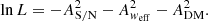
CHIME is a transit radio telescope operating across the 400−800 MHz band. It is an excellent FRB detector, owing to its large field of view, wide bandwidth, and high sensitivity, plus its powerful correlator (CHIME/FRB Collaboration 2018). During pre-commissioning, it detected 13 new FRBs (CHIME/FRB Collaboration 2019). The CHIME/FRB Catalog 1 was next published in June 2021 (CHIME/FRB Collaboration 2021), containing 536 FRBs, of which 474 are one-off bursts and 63 are bursts from 18 repeating sources. The catalog spans observing dates from 2018 July 25 to 2019 July 12. In the current work, we started by limiting ourselves to first reproducing the bursts that are classified as one-off FRBs. We stress that frbpoppy is capable of simulating repeating FRBs too (Gardenier et al. 2021), and we will pursue that study in future work. The catalog is the first set numbering over 100 FRBs from a single telescope. That is important because such a set is governed by uniform selection effects. These selection effects imposed by the differences in hardware and in search algorithms (Rajwade & van Leeuwen 2024) determine, in large part, the overall parameter distributions that describe the observed sample, for e.g., the dispersion measures (DMs), distances, bandedness, and pulse widths. In Figs. 1 and 2 we compare two such parameter distributions – DM and signal-to-noise ratio (S/N) respectively – for CHIME/FRB against those of the pre-existing FRB population discovered by other telescopes. We here do this as a first impression, to outline the biases at stake, and investigate these distributions in more detail later. The DM distributions are relatively similar. That is interesting because CHIME/FRB operates at a lower frequency than most other surveys, which would generally make higher-DM sources especially hard to find. Especially at these low frequencies, such sources suffer more from intra-channel dispersion and scatter broadening than low-DM FRBs. This disadvantage is possibly mitigated by other relative advantages of the CHIME/FRB system (its narrow channels might, for example, sufficiently limit the intra-channel dispersion). It is also possible that other biases, working against low-DM sources instead, balance out the selection effects with DM. Hints for the latter are reported by Merryfield et al. (2023), who find that the CHIME/FRB pipeline selects against bright, low-DM FRBs. We investigate this in Sect. 5.4.
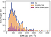 |
Fig. 1. DM distribution histogram of one-off FRBs in the TNS database. The total sample of FRBs is shown in blue while those from CHIME/FRB and other telescopes are shown in orange and green respectively. |
For the S/N, the CHIME/FRB distribution is shifted toward higher values than that of the other telescopes. This could be intrinsic, a result of stricter confidence level requirements, or a combination thereof.
2.2. Modeling underlying populations
As the number of detected FRBs increases, a number of sources have shown complex behavior or circumstances. Our goal is to distill the most important trends from the complicated real FRB population. We thus used a number of parameters to model its main characteristics, both source-related properties (luminosity, pulse width) as well as population-related properties (number density, DM). Here, we describe the parameter distribution models adopted in our simulations (see Gardenier et al. 2019 for further details on these methods). For reference, the parameters and their meaning are also listed in Table A.1.
2.2.1. Number density following a power-law model
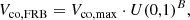
In frbpoppy, a number of different models can establish the number-redshift relation dN/dz of intrinsic FRB populations per comoving volume. In this study, we focused on two models. The first tracked the cosmic star formation rate (SFR), as we discuss in the next subsection. In the second, we created a power-law model that does not depend on SFR. In this case, frbpoppy modifies the uniform sampling U(0, 1) with exponent B
 (1)
(1)
where B determines the slope of the cumulative source-count distribution for detected FRBs, above a certain peak flux density detection threshold, at the high flux density end. The parameter α is introduced via
 (2)
(2)
In a Euclidean universe, where the FRB count per comoving volume element does not evolve with redshift, we have B = 1 and α = −3/2. By introducing α via this power-law index, it is the same as the log N − log S slope in the high fluence limit. From now, we use the term Euclidean model to refer to such non-evolving models with α = −3/2. As a number of studies have suggested or reported deviations from α = −3/2 (e.g., α = −2.2 in both James et al. 2019 and GL21) we do however search for the best-fit value of α in a number of experiments reported in Sect. 4.1.1.
2.2.2. Number density following a star formation rate model
There is ongoing discussion on whether the FRB event rate tracks the SFR. James et al. (2022b) find it does. Zhang et al. (2021) and Zhang & Zhang (2022), however, claim that the FRB population as a whole does not track the SFR; while a delayed SFR model, potentially caused by compact binary mergers, cannot be rejected with the ASKAP and Parkes sample. So, in this work, we considered both the SFR itself, plus delayed SFR models with three different delay times: 0.1, 0.5, and 1 Gyr. We note that for delay time distribution (DTD), we used a constant model, which assumes all compact binaries have the same delay time τ (while Zhang et al. 2021 mention various other DTDs, including power-law, Gaussian or log-normal). We discuss the results in Sect. 4.1.2 and Sect. 4.1.3.
2.2.3. Spectral index
The spectral index γ (Eq. (10) in Gardenier et al. 2019; called si in GL21) describes the relative flux density at different frequencies within the spectrum. In frbpoppy, this index acts through converting the FRB fluence into the observing bands of the modeled surveys (see Eq. (8) describing Speak). It is arguably best constrained by comparing FRB fluences and rates from survey at different frequencies. Such multi-survey simulations are one of the strong points of frbpoppy and we will explore this aspect in future work. In the current work, however, we only modeled CHIME/FRB, effectively at a single frequency band. In this case the resulting γ is greatly influenced by the choice of vlow, vhigh, and the assumption that the power-law relationship (Eν ∝ νγ) holds throughout the whole frequency range. As this degeneracy cannot be solved in a single-frequency study, we did not treat γ as a free parameter here while we formally defined it as γ = −1.5. This value is motivated by the mean spectral index found by Macquart et al. (2019) using a sample of 23 FRBs detected with ASKAP.
2.2.4. Luminosity
The bolometric luminosity Lbol was generated from a power-law distribution with power-law index li and range [Lmin, Lmax]. Such a range limit is the simplest method to bound the allowed luminosity values and keep the function convergent. Physically, it suggests there is some minimum required energy to produce an FRB (similar minimum physical luminosities have been proposed for pulsars, see e.g., van Leeuwen & Stappers 2010 and references therein) and some maximum available energy reservoir per burst. Since the publication of GL21, the detection of FRB 20220610A has raised the maximum observed rest-frame burst luminosity to 1046 erg s−1 (Ryder et al. 2023), so we have increased Lmax to the same value. Inferred luminosities depend on the assumed bandwidth of emission; so some caution is required when comparing these numbers. To provide context to this extreme luminosity, we note that the magnetic Eddington limit of a strong-field (> 3 × 10¹⁴ G) neutron star is 1042 erg s−1 (Thompson & Duncan 1995). Whether a lower limit to the one-off FRB luminosity exists is unclear. The ∼1037 erg s−1 luminosity of nearby repeating FRB 20200120E (Bhardwaj et al. 2021) already indicates the underlying process, if the same, can operate over a range of brightness. To limit computing time our simulations require a lower bound though, and for the one-off FRBs under consideration here, we chose Lmin = 1041 erg s−1. This is 3 orders of magnitude below the least luminous localized one-off bursts, such as FRB 190608 (Macquart et al. 2020) at ∼1044 erg s−1 (although given the current state-of-the art, only relatively bright FRBs can generally be localized). As it is also conservative compared to the Lmin = 7 × 1042 erg s−1 suggested by Cui et al. (2022) for their CHIME/FRB non-repeater sample, we are confident our simulation coverage is complete.
The luminosity we model in frbpoppy represents the isotropic bolometric radio luminosity. In contrast to similar studies for pulsars (e.g., van Leeuwen & Verbunt 2004) we did not (yet) include beaming effects for FRBs, given the uncertainly of the progenitor models in this regard. We discuss this in more detail in Sect. 5.2.
Other luminosity functions exist, and could potentially be implemented in the future. Once the number of detected FRBs allows for it, one could then distinguish between multiple luminosity models. Luo et al. (2020), for example, consider a Schechter luminosity function. We do note here that the original strength of this function – for galaxies – was that it was derived from self-similar galaxy formation models, and next well described the observed galaxy distributions (Schechter 1976). Its current application to FRBs, in contrast, is ad hoc, and similar to application of a generic broken power law. Both functions still require an Lmin lest they diverge at the low-luminosity end. Testing a log-normal distribution might also be interesting. Considerations on the luminosity functions in frbpoppy are discussed in more depth in Gardenier et al. (2019).
2.2.5. Pulse width
The intrinsic pulse width wint is modeled with a log-normal distribution
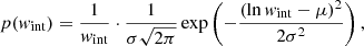 (3)
(3)
where μ, σ are related to the input parameters wint, mean and wint, std by wint, mean = exp(μ+σ2/2) and ![Mathematical equation: $ \mathit{w}_{\mathrm{int, mean}}=\sqrt{[\exp(\sigma^2)-1] \exp(2\mu+\sigma^2)} $](/articles/aa/full_html/2024/10/aa50673-24/aa50673-24-eq4.gif) .
.
The pulse width warr of an FRB arriving at Earth is
 (4)
(4)
The observed pulse width is
 (5)
(5)
where tscat is the scattering time while tsamp and tDM are the result of instrumental broadening. In our simulation, a log-normal distribution for tscat is adopted (see Fig. 14, right panel); tsamp is 0.98304 ms as in CHIME/FRB Catalog 1; and tDM is the intra-channel dispersion smearing the CHIME/FRB back-end incurs for each FRB.
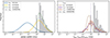 |
Fig. 14. Probability distribution of pulse width and broadening effects. Left panel: normalized distribution of intrinsic pulse width wint, for the intrinsic, generated sample and for the surveyed, detected sample, the effective pulse width weff of this surveyed sample in the simulation, and of the CHIME/FRB Catalog 1 widths. Right panel: distribution of the simulated normalized tdm and tscat subcomponents of the width of the surveyed, detected FRBs; compared to the values from the CHIME/FRB Catalog 1. The sampling time tsamp of 0.98304 ms is marked with a dashed line. The population is generated using best-fitting values for the 0.1-Gyr delayed SFR model. |
2.2.6. Dispersion measure
The total DM of an FRB is
 (6)
(6)
where DMhost is the host galaxy contribution (including the circumburst environment contribution DMsrc and Milky Way halo contribution DMMW, halo) in the source rest frame. We generated DMhost using a log-normal distribution (lnDMhost ∼ N(σ, μ)), where input parameters DMhost, mean and DMhost, std represent the mean and standard deviation of the log-normal distribution respectively; DMMW is the Milky-Way interstellar medium (ISM) contribution obtained from the NE2001 model (Cordes & Lazio 2002).
The intergalactic medium (IGM) contribution DMIGM is estimated using a linear relation with redshift DMIGM ≃ DMIGM, slope z (Zhang 2018; Macquart et al. 2020), around which we include the spread from a normal distribution, leading to
 (7)
(7)
As the value of DMIGM, slope derived in Macquart et al. (2020, their Fig. 2) is ∼1000 pc cm−3, and the lower limit on their 90%-confidence interval is ∼700 pc cm−3, we set the lower limit in our MCMC parameter search space to be 600 pc cm−3. We discuss a number of implications from our simulation for the DMIGM model in Sect. 5.
2.3. The CHIME/FRB detection system model
Using frbpoppy, we first generated simulated intrinsic populations according to certain parameter distribution models. We then set up “surveys” with survey parameters for specific telescopes. We applied each survey to each intrinsic population, selecting the events that meet the S/N threshold to form detected populations. We compared the simulated detected populations to the actually detected population. From the best match, we inferred the actual intrinsic population (as in Gardenier et al. 2019). A straw man CHIME survey was previously included in frbpoppy (Gardenier et al. 2021). In Sect. 5.5 we evaluate the actual sensitivity of the telescope compared to these estimates. Furthermore, in this work we used the implemented number of channels (16k), and an improved beam model.
2.3.1. The beam model
The earlier, initial approximation of the CHIME primary beam in frbpoppy consisted of a North-South cosine function convolved with an East-West Airy disk pattern. The behavior of the synthesized beams formed in subsequent stages is more straightforward, and well known. Since then, a CHIME primary-beam pattern measurement was empirically derived from the telescope response to the Sun (Amiri et al. 2022). Using the accompanying cfbm package3, we now included this improved CHIME/FRB beam intensity at 600 MHz in frbpoppy. The implemented beam model is shown in Fig. 3, left panel, with the East-West slice (y = 0°) and North-South slice along the meridian (x = 0°) shown in upper right and bottom right panels respectively.
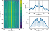 |
Fig. 3. CHIME/FRB beam model reproduced with cfbm at 600 MHz. The left panel shows the beam intensity map in the range [ − 40° ,40° ] (East-West) and [ − 60° ,60° ] (North-South). The upper and bottom right panels show the East-West slice (y = 0°) and North-South slice along the meridian (x = 0°) respectively. The relative beam intensity is dimensionless, and normalized to the transit of Cyg A (Amiri et al. 2022). To include the side-lobe in our simulation, the beam range [ − 15° ,15° ] (East-West) × [−60° ,60° ] (North-South) is considered, where the East-West borders are indicated with dash-dotted lines. |
Although only three one-off FRBs are detected outside the main beam (|East-West offset| > 2.0°) in CHIME/FRB Catalog 1, this side-lobe detection fraction is important to distinguish models with different redshift distributions and luminosity models. The main-lobe and side-lobes arguably deliver both a deep and a shallow survey. Therefore, we did not restrict ourselves to the main beam but we consider the East-West range of [−15°, 15°]. We end before the significant drop in intensity beyond that range. These borders are indicated with dash-dotted lines in Fig. 3. Although the far side-lobe of the CHIME/FRB beam is yet poorly understood (CHIME/FRB Collaboration 2021) and the three side-lobe events (FRB 20190210D, FRB 20190125B, and FRB 20190202B) are excluded in many statistical studies, they are included in our simulations, as we expect them to put significant constraints on the number density models, luminosity distributions and high S/N events.
2.3.2. Modeling CHIME surveying
In the surveying step, the S/N of an FRB is derived from its peak flux density  and pulse width. This peak flux density (Lorimer et al. 2013; Gardenier et al. 2019) is
 (8)
(8)
where  GHz, and
  MHz, v2 = 800 MHz and v1 = 400 MHz are adopted; γ notates the spectral index; D(z) = dL(z)/(1 + z) is the proper distance of the source; and the luminosity distance dL(z) is calculated with
 (9)
(9)
where we used Planck15 results H0 = 67.74 km s−1 Mpc−1, Ωm = 0.3089 and ΩΛ = 0.6911 for a flat Lambda cold dark matter (ΛCDM) universe (Planck Collaboration XIII 2016)4. The S/N is derived using
 (10)
(10)
where I is the beam intensity at the detection location, G is the gain, β is the degradation factor, Tsys is the total system temperature specific to CHIME/FRB, npol is the number of polarizations, and ν1, 2 are the boundary frequencies of the survey, respectively (Lorimer & Kramer 2004). For the CHIME/FRB gain, degradation factor and total system temperature we updated the preliminary numbers used in Gardenier et al. (2021) and follow Merryfield et al. (2023). The measured system equivalent flux density (SEFD) reported there ranges from 30 to 80 Jy over the band. Merryfield et al. (2023) initially used a value of 45 Jy in their injection system but find their idealized assumptions do not represent the system adequately; requiring an increase of the injection threshold from 9σ to 20σ. We here aim to include this real-life factor of 2 over the theoretical performance for an SEFD of 45 Jy by using the average SEFD reported over the band (55 Jy, implemented as gain G = 1 K Jy−1 and Tsys = 55 K) and a degradation factor β of 1.6. We discuss the influence of these updated numbers in Sect. 5.5.
Up to and including frbpoppy 2.1 the S/N formula, Eq. (10), erroneously used warr (Eq. (17) in Gardenier et al. 2019), not weff, for the observed pulse width. This meant that while  was correctly decreased by the factor warr/weff in Eq. (8), the accompanying, partly counterbalancing increase in S/N by
  in Eq. (10) was not properly accounted for. This made smeared-out pulses harder to detect than in real life. That is corrected in frbpoppy 2.2 and in our results below. The impact of this change is, for example, that higher-DM FRBs are slightly easier to detect, influencing α. To determine the impact of the change, we compared the best-fit Euclidean models against it, and find that the values describing the underlying population (Table 1) changed by about 0−0.4σ.
Summary of best-fitting values for different models in this work and GL21.
2.3.3. Comparisons with the CHIME/FRB injection system
Part of our approach is similar, in goals and method, to the CHIME/FRB injection system mentioned above (Merryfield et al. 2023). There, a mock population of synthetic FRBs was injected into the real-time search pipeline to determine the selection functions. Our main goal with frbpoppy is to next go beyond this essential expression of the selection functions: we focus on determining the intrinsic population distributions, and we argue that the best way to include the relevant biases imposed by the Universe and telescope is through forward modeling.
In contrast to using the selection functions or fiducial distributions from CHIME/FRB Collaboration (2021) or Merryfield et al. (2023), the flexibility of forward modeling allows us to determine which selection factors contribute most, thus leading to better understanding of the interaction between the intrinsic population and the telescope strengths and weaknesses. This is only possible if the survey is modeled in the same simulation as the population. Furthermore, certain parameters – e.g., the spectral index, the activity dependence on frequency – can only be done in a multi-survey simulation, which means one has to treat selection effects similarly for all.
3. Methods
Our aim is to find the global best-fit model for describing the FRBs emitted in the Universe, which are then input to the modeled telescope. The sample of bursts can be well described by of order 10 characteristic numbers. A fit over such a large number of parameters is, however, computationally challenging. To realize this after all, we have improved frbpoppy code and application in three ways. We first added MCMC sampling, we next employed data reuse where possible, and we finally deployed frbpoppy on a supercomputer. These are described below.
3.1. Markov chain Monte Carlo
Gardenier & van Leeuwen (2021, GL21) conducted a multi-dimensional MC simulation over 9 parameters, all explained above: α, γ5, li, Lmin, Lmax, wint, mean, wint, std, DMIGM, slope, and DMhost. Due to computational limitations, in that work these these 9 parameters were divided over 4 subsets, chosen to be maximally independent of each other, but with a few shared parameters between sets, such that the globally best model could arguably be approached: 1: {α, γ, li}, 2: {li, Lmin, Lmax}, 3: {wint, mean, wint, std} and 4: {DMIGM, slope, DMhost}. Each time, one subset was searched, keeping other parameters fixed, using the best-fitting values of previous run as the input of the subsequent run. This was repeated over multiple cycles to approach the global optimum. Fig. 4 serves as an example of the three-dimensional goodness-of-fit (GoF) plot from such an frbpoppy MC simulation; in this case for {α, γ, li}. A down side of this approach, also discussed in GL21, is that during every run the uniform sampling means regions of low and high GoF are treated equally, and searched with the same step size. Thus, the MC simulation spends a considerable amount of computing time in regions that are not actually interesting.
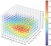 |
Fig. 4. Three-dimensional GoF plot for {α, γ, li} from an MC simulation. Different GoFs are denoted with colors as well as marker sizes. |
Therefore, we implemented and conducted a full dimensional MCMC simulation6, to supersede the GL21 MC simulation with divided subsets. As the MCMC sampler moves out of regions of poor GoF more quickly than the brute-force method employed earlier, this allows us to sample the full multi-dimensional search space. Additionally beneficial is that such sampling allows for error estimates on the outcome values, something the previous, subset implementation lacked.
For a given set of input parameters, we first generated a small population of 106 FRBs, then followed these through our CHIME/FRB representation, and saved the detected FRBs to the surveyed population. Like in Gardenier et al. 2019, we used the terms “surveyed”, “observed” and “detected” synonymously. We repeated the process until we had enough FRBs (e.g., 1000) in the surveyed population. To limit the computational time required when sampling poor regions, we also stopped if after a certain number of iterations we did not have enough detections.
GL21 use the p-value pK − S from the two-sample Kolmogorov–Smirnov (K–S) test as GoF in their MC simulation, to evaluate which population is more similar to the observed population. The growing size of the observed sample, however, means the high S/N or high DM events are approaching the actual boundaries of the population. Since the models or parameters we are trying to constrain make different predictions for these boundaries, the outlier events can be of great significance to evaluate population models. Therefore, we have extended frbpoppy with the option to use the k-sample Anderson-Darling (A–D) test (Scholz & Stephens 1987) as the measure to determine the GoF. The statistic A2 of the A-D test uses weighting functions when it sums the cumulative distribution function (CDF) distances between samples, giving more weight to the tail of distributions. In maximum likelihood estimation (MLE), the log-likelihood function then is the negative of the loss function (the statistic)
 (11)
(11)
To represent the main features of FRB populations, we compared the S/N, weff and DMtotal distributions from a simulation with the CHIME/FRB Catalog 1 one-off FRBs7. To combine these three distributions to constrain the parameter set, we used as the log-likelihood function lnL the sum of the three statistic Ai2
 (12)
(12)
Here, we assume that the three distributions are uncorrelated, and that when lnLmax is reached, we have identified the joint minimum of AS/N2, Aweff2 and ADM2. We used lnL (i.e., −∑Ai2) as the total GoF to evaluate how well a set of parameters within the specific model reflects the simulated samples match real observations. We discuss these statistics more in Sect. 5.10.
3.2. Speeding up of frbpoppy
In order to feasibly operate frbpoppy within an MCMC, a number of code optimizations and changes were implemented, to speed up the generation of large populations. We now use numpy array look-up methods, superseding the SQL database approaches used in frbpoppy 2.1.0 (Gardenier et al. 2019), to query the DMMW and the cosmological distance dL. With numpy.searchsorted, we can efficiently find the indices where elements (coordinates or redshifts) should be inserted into a sorted one-dimensional array and then use indexing to obtain the required DMMW or dL
A population in frbpoppy contains property values for e.g., distance, luminosity, pulse width and DM. When generating a new population, frbpoppy now has the option to reuse some of these quantities. This is especially beneficial for values that are expensive to generate but are uncorrelated with other values. In this way, run time can be reduced by ∼50%. Under this mode, we started from a relatively small population (106 FRBs) for which all parameters are drawn from the selected model. In the simulated population, the redshift z, distance dco, coordinates (gl, gb), and dispersion measure (including DMhost, DMIGM and DMMW) are coupled. They should be reused as a whole. On the other hand, the FRB-intrinsic properties, i.e., the luminosity Lbol, and pulse width wint are independent of this first set, and can safely be regenerate from the parent distribution. These create new FRBs that are not meaningfully correlated with those in the genesis population. All small populations thus generated are next merged to form a large population (hereafter, the combined population). This means that each set (z, dco, gl, gb, DMhost, DMIGM, and DMMW) is used N times in the large population, combined with different Lbol and wint. To validate this approach, we generated surveyed populations both with and without reusing these quantities, and find they are practically identical, with similar K–S test p-values (see, e.g., Fig. 5). Fewer than 1% of FRBs have identical coordinates and redshifts. As a further check, we compared full MCMC runs of the Euclidean model with and without reusing quantities, and found no significant differences in the best-fitting values. Hence, the new strategy is robust and does not influence our detection of FRBs.
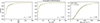 |
Fig. 5. Cumulative distribution plots of S/N, weff and DMtotal distributions from two surveyed populations generated with and without reuse, for the Euclidean model. The p-value of K–S test is also shown for reference. |
We employ this reuse and the other optimizations in the results discussed in the remainder of the paper. Using these improvements, frbpoppy 2.2.0 generates a population about 20 times faster than frbpoppy 2.1.0.
3.3. Computations
The computations were carried out on the Dutch national supercomputer Snellius8, using the 128-core “thin” or “rome” nodes. For our default MCMC simulation of 240 nwalkers × 500 steps, the computational cost is 2 − 8 × 10⁴ core hours, depending on the FRB population models and beam intensity map.
4. Results
Below we present the outcomes of our MCMC simulations. The interpretation is covered in Sect. 5.
4.1. Best-fitting parameters from different number density models
4.1.1. Power-law number density model
The confidence contours and marginalized likelihood distributions for the power-law number density models are shown in Fig. 6 and the best-fitting values with 1σ uncertainties are listed in Table 1, for the population parameter set {α, li, log10wint, mean, wint, std, DMIGM, slope, DMhost, mean, DMhost, std}.
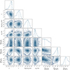 |
Fig. 6. Confidence contours and marginalized likelihood distributions for the 7 parameters in our power-law number density model. |
While the number density power-law index α was −2.2 in the best overall model from GL21, we now find  from the full MCMC. That value is consistent with the non-evolving Euclidean distribution (cf. Oppermann et al. 2016; James et al. 2019). We thus hereafter refer to this best-fit power-law density model as the Euclidean model. The luminosity index li is constrained to
  ; and we discuss this finding, and compare it with other results – minding the different definitions – in Sect. 5.6. For pulse width, the best-fitting values of log10(wint/ms) is
  . This produce mean intrinsic pulse widths two orders of magnitude higher than in GL21 – this difference is explained in Sect. 2.3.2.
For the components that contribute to the DM, we find the DMIGM, slope is  pc cm−3 while the DMhost, mean, DMhost, std are
  pc cm−3 and
  pc cm−3 respectively. We note here that the mean and standard deviation of DMhost describe a log-normal distribution; hence, they are quite far away from the more meaningful median value. After conversion, the median of the observed distribution for DMhost is ∼330 pc cm−3 and its probability density function (PDF) peaks at ∼130 pc cm−3 (both in the source frame). These values are larger than what Zhang et al. (2020) find from the IllustrisTNG simulation and Yang et al. (2017) from a sample of 21 FRBs. It is worth noting that the DMsrc and DMMW, halo contributions are absorbed into the DMhost term in the simulations. DMMW, halo is not explicitly modeled in NE2001 (Cordes & Lazio 2002, 2003). Prochaska & Zheng (2019) estimated DMMW, halo ∼ 50 − 80 pc cm−3. Yamasaki & Totani (2020) reported a mean value of DMMW, halo ∼ 43 pc cm−3. For simplicity, in the following discussions and in Fig. 15 in this work, we adopted a typical DMMW, halo of 40 pc cm−3 and subtracted it from the reported DMhost results.
4.1.2. SFR model
We described the SFR model using parameters similar to the power-law density model (above) but without requiring a number density power-law index α, leading to the 6-parameter set {li, log10wint, mean, wint, std, DMIGM, slope, DMhost, mean, DMhost, std}. The confidence contours and marginalized likelihood distributions are shown in Fig. 7 while he best-fitting values with 1σ uncertainties are also listed in Table 1. The constraints on {li, log10wint, mean, wint, std} are very close to those of the Euclidean model; however, noticeable differences exist in {DMIGM, slope, DMhost, mean, DMhost, std}. The median of observed source frame DMhost is ∼279 pc cm−3 and its PDF peaks at ∼105 pc cm−3. This is larger than the median value 179 ± 63 pc cm−3 found in Mo et al. (2023) for their SFR model.
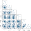 |
Fig. 7. Confidence contours and marginalized likelihood distributions for the 6 parameters in our SFR model. |
In Fig. 7, the slightly diagonal confidence contours in the subpanels that project DMIGM, slope against the DMhost parameters indicate that the DM contributions of the IGM and the host are somewhat degenerate with each other. This is because the DM excess (DMtotal − DMMW) is supplied by the combination of DMIGM, slope z and DMhost/(1 + z). Models that produce fewer local FRBs, like the SFR model, thus require a larger DMIGM, slope and a smaller DMhost to fit the observed distributions, compared to the Euclidean model.
4.1.3. Delayed SFR model
To investigate the impact of formation channels that are delayed with respects to the SFR, we simulated models with three different delay times, of 0.1 Gyr, 0.5 Gyr and 1 Gyr. In these models, the number of present-day, local FRBs is determined by the SFR when the delay process commenced. As the recent SFR declines steeply (see e.g., Gardenier et al. 2021), the number of local FRBs is expected to increase with longer delay times. FRBs with a delay time of 1 Gyr were formed near z ≃ 0.1, where the SFR was ∼30% higher. Thus, models with longer delay times in principle contain more low-z FRBs; or, reciprocally, such models require a lower source density to produce the number of FRBs that are observed. As the simulated detection numbers in frbpoppy are scaled to the actually detected number, we cannot easily identify an overall increase in the number of local FRB sources. The GoF would only be affected if there was a significant change in slope within the sampled redshift range. This effect is visible in the zoomed-in plot in the right panel of Fig. 8, where the shapes of the three SFR models resemble one another very closely. These are normalized to the same number of detections; the differences only emerge in the underlying physical rate. The posterior probability distributions are shown in Fig. 9. As all four SFR models have very similar best-fitting values, we cannot confidently distinguish between these. We thus corroborate the conclusion from Shin et al. (2023) that there is insufficient evidence in CHIME/FRB Catalog 1 to strongly constrain how FRB evolution follows the SFR. There is, however, so-called strong evidence (Raftery 1995) in the Bayesian Information Criterion (BIC) in favor of the SFR models over the Euclidean model (Table 2). This conclusion differs from Zhang & Zhang (2022), who prefer a significant lag: a log-normal delay model with a central value of 10 Gyr and a standard deviation of 0.8 dex.
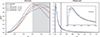 |
Fig. 8. Probability distributions of FRBs as functions of redshift for different models. Left panel: probability density functions (PDFs) of the intrinsic FRB population versus redshift, for the Euclidean, SFR and delayed SFR models with three delay times. The redshift range [0, 1.5] is used in our simulation. For information, we also show the region [1.5, 2.5], gray shaded, such that the shift of the SFR peak is visible between the models. Right panel: simulated observed FRB population PDFs against redshift, for the same models. The mean redshift ⟨z⟩ for the different models are marked by the dashed vertical lines. An unfilled zoomed-in view of the redshift range [0, 0.2] is also shown. |
 |
Fig. 9. Confidence contours and marginalized likelihood distributions for three delayed SFR model (0.1, 0.5, 1.0 Gyr). |
Summary of the A-D statistic and BIC for different models.
4.2. Reproducing CHIME/FRB distribution and model comparison
With the best-fitting values from the MCMC, we reproduced the FRB populations and surveyed them with our model of CHIME/FRB. The CDF of S/N, w and DMtotal are shown in Fig. 10. The CHIME/FRB Catalog 1 distributions are also shown for comparison. The CDF curves of weff show good agreements with CHIME/FRB while those of S/N has the largest discrepancy for all models. The overall good reproduction of all three distributions supports the method that we sum the A-D statistics to construct the log likelihood function.
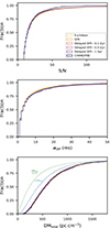 |
Fig. 10. Comparison of cumulative distributions for simulated populations with best-fitting parameters and the CHIME/FRB Catalog 1 one-off FRBs. The S/N, weff and DMtotal are shown in upper, middle and lower panels respectively. The population coloring is the same in all subplots. In the DM plot we also show the cumulative contributions of DMhost/(1 + z), and of the additional DMIGM, for the delayed SFR model with 0.1 Gyr. These show how, for the lower-DM half of the population, these two components contribute roughly equally to the DMtotal; while for the higher-DM half, the host contribution dominates. |
To compare the models, we used the BIC (mentioned above):
 (13)
(13)
where k is the number of free parameters in the model, n is the number of samples. In the power-law density models, k = 7; in the SFR and delayed SFR models, k = 6. A summary of the A-D statistic and BIC for different models is provided in Table 2. Raftery (1995) list that BIC differences between 0−2, 2−6, and 6−10 correspond to “weak”, “positive” and “strong” evidence respectively. To avoid over-interpretation, we referred to BIC differences between 0−2 as only a hint of evidence. Therefore, the three delayed SFR models, with almost the same BICs, show a hint of evidence over the SFR model; and all four are strongly favored over the power law density models in general, and hence also over their most favored case, the Euclidean model. The power law density model produces the least favorable fit, especially in the S/N distribution.
5. Discussion
Our results provide new insights into how many FRBs are born in our local universe and their evolution, into the brightness and emission of the bursts, and into the baryonic material between the emitters and Earth. These warrant discussion and interpretation. We provide this below, ordered from more general to more expert topics.
5.1. The number of FRBs in the local Universe
Using frbpoppy and the CHIME/FRB Catalog 1 we can establish of how many FRBs are born and go off per day in our local Universe, which we define to be up to z = 1. We here consider FRBs purely as an observable phenomenon. Implications for any underlying progenitor numbers are covered in the next subsection. We present this fiducial number here to provide a best estimate based on our simulations. The number depends on the model parameters (as discussed above) and readers are invited to run their own simulations if desired. They can also directly download this snapshot as described in Sect. 5.12.1. We used our best-fit no-delay SFR model (with spectral index −1.5, luminosity index −1.58, and minimum luminosity 1041 erg s−1). We inputed the CHIME/FRB rate of  for fluence > 5 Jy ms, scattering time < 10 ms at 600 MHz, and DM > 100 pc cm−3.
From these we determine the rate of non-repeating FRBs that happen in the z < 1 volume: 108.3 ± 0.4 day−1. In other words, out to z = 1, between 4 ± 3 × 10³ FRBs go off every second.
5.2. Implications for the FRB progenitor volumetric rate
The FRB frequence determined in the previous subsection corresponds to an averaged volumetric rate density ρ of 2 × 10⁸–1 × 10⁹ Gpc−3 yr−1. If one assumes FRB emission is concentrated with a beaming fraction fb (the fraction of the sky that is illuminated by the emitter beam), then the FRB source rate is a factor 1/fb higher than this FRB rate. On the other hand, the input energy is emitted in a more focused way. If we presume that the emission is uniform across the beam we can then convert the isotropic luminosity into a beamed luminosity via L′bol = Lbol, iso/fb. This increased luminosity means FRBs are observable over a larger volume; and this effect actually outperforms the sky illumination effects. In our simulations, lowering the beaming fraction thus reduces the required underlying source rate.
Our rate is significantly higher than straightforward volumetric rates such as those quoted in Nicholl et al. (2017) as  Gpc−3 yr−1, and other early direct estimates. These large apparent discrepancies arise because such work only takes the observed FRBs into account for their rates. The aim in frbpoppy is to carry out forward modeling, and correctly recover the intrinsic-to-observed selection, as shown in Fig. 8. Only then can one aim to determine the underlying FRB formation rate from the telescope-observed rates. The low-luminosity part of the underlying FRB population dominates the rate, while these are only rarely detected.
The strength of frbpoppy is its FRB population synthesis. In future work, we will extend this to include progenitor populations; while those who currently study certain progenitor types, could aim to produce the rates from Sect. 5.1. Still, a number of order-of-magnitude conclusions can already be drawn here.
We first investigate if double neutron star (DNS) mergers occur in sufficient numbers to produce our inferred FRBs. If we assume the radio FRB fb is similar to the high-energy beaming fraction, then we can use typical fb = 0.04 found in short-duration gamma-ray bursts (GRBs; Fong et al. 2015). The observed FRB rate would require a local volumetric DNS rate ρ ≃ 6 × 10⁷ − 3 × 10⁸ Gpc−3 yr−1. This far exceeds the local DNS coalescence rate of 1540 Gpc−3 yr−1 derived from GW170817 (Abbott et al. 2017). As a matter of fact, none of the cataclysmic progenitor models suffice (see, e.g., Ravi 2019).
As mentioned before, we aim to analyze the CHIME repeater FRBs in future studies; but even if most apparent one-off FRB sources are very infrequent repeaters such emission of multiple FRBs over the progenitor lifetime can greatly alleviate the rate problem. GL21 identify magnetars as the progenitors to FRBs. We first focus on younger magnetars, where the beaming fractions are high (see e.g., Straal & van Leeuwen 2019). Using the fb = 0.2 found for Galactic radio magnetars (Lazarus et al. 2012), we find an FRB emission rate of 1 − 7 × 10⁸ Gpc−3 yr−1. If we take an average supernova rate out to z = 1 of 3 × 10⁵ Gpc−3 yr−1 (Melinder et al. 2012), a magnetar fraction of 10−1 (Keane & Kramer 2008), and an activity lifetime of 103 yr, each source would need to produce 𝒪(10) bursts per year – almost all of which can be at the low-luminosity end. We conclude this rate is possible. If sources are older, longer-period magnetars (cf. Bilous et al. 2024), the much larger active lifetime and the smaller beaming fraction work together toward even more attainable rates.
5.3. How FRB formation trails the SFR
In our models, the scenario where FRBs follow the delayed SFR is slightly favored over no delay (Table 1). This agrees with the findings of James et al. (2022b), but is in contrast with Zhang & Zhang (2022). As all SFR-based models are strongly favored over Euclidean models, our results indicate that FRB emitters must be the direct descendants of a stellar population. Source classes such as neutron stars, magnetars (CHIME/FRB Collaboration 2020a; Bochenek et al. 2020), and stellar mass black holes fit this description. Coalescing neutron stars generally take a much longer time to merge (e.g., Pol et al. 2019). Still we know of one FRB in an environment long devoid of star formation: FRB 20200120E, in a globular cluster of M81 (Bhardwaj et al. 2021; Kirsten et al. 2022). That example means we should consider the possibility there is some fraction of FRBs that does exhibit a delay. Proposed models for FRB 20200120E are induced collapse of a white dwarf through accretion (accretion-induced collapse, AIC), or from the merger of two white dwarfs (merger-induced collapse, MIC). In such models, the white dwarf inspiral is driven through gravitational-wave energy losses originally, and finally through mass transfer. Kremer et al. (2023) find that after 9 Gyr, the approximate age of the M81 globular cluster, white-dwarf mergers continue to occur, forming young neutron star that are the FRB emitters; although the relatively low rate requires a long, 105 yr active emitter lifetime. Whatever the model, FRB 20200120E exists and its formation trails the SFR peak by billions of years. It would be interesting to determine how many such FRBs can be mixed in with a general population of FRBs that does closely follow the SFR. To investigate this, we created a hybrid intrinsic population, of which 90% of the FRBs follow SFR immediately, while the other 10% are deferred by 1 Gyr. Hence, these FRBs have a mean delay time of 0.1 Gyr. Although the hybrid population has more low-z events, it hardly deviates from the purely 0.1 Gyr delay mode in our results. We conclude that the average delay time is the most important parameter. As our models slightly favor short delay times, the fraction of deferred FRBs cannot be large. This can be quantified through the scenarios based on the summary in Table 1. For example, if a fundamentally no-delay population contains a fraction fd FRBs formed with delay time τd, then the BIC improves by 1.6 if  , but then worsens again by 0.1 when
  .
.
Other ways to elucidate the connections between FRBs and star formation exist in principle. From the locations of 8 FRBs within their host, Mannings et al. (2021) find no convincing evidence that FRBs strictly follow star-formation, nor that they require a delay; and an FRB survey with Low Frequency Array (LOFAR) in star burst galaxy M82 finds no bursts (Mikhailov & van Leeuwen 2016).
5.4. Side-lobe detection fraction
As discussed in Sect. 2.3.1, CHIME effectively performs a deep (main-lobe) and shallow (side-lobe) survey simultaneously. The side-lobe plateau incorporated in our simulations ranges over ±15° (East-West) and is thus significantly larger than the main-lobe, as that roughly spans ±2° (Fig. 3). On average, this side-lobe region under consideration is over a 100× less sensitive than the peak sensitivity. Any FRBs detected there must be very bright; and other such bright FRBs must then also occur in the main-lobe, where they are seen as high-S/N bursts (see, also, Lin et al. 2023). The 3 side-lobe FRBs reported in CHIME/FRB Catalog 1 have S/Ns of 21, 20, and 13. We would thus also expect ∼1% of main-lobe FRBs to have S/Ns 100× higher, of 103–104. And yet, the highest S/N detected in CHIME/FRB Catalog 1 is only 132.
We thus conclude that the CHIME/FRB pipeline missed a significant number of very bright FRBs. We would expect these bursts to be relatively nearby and hence, display low DM. Merryfield et al. (2023) mention that the CHIME/FRB pipeline has a bias against such bright, low-DM FRBs through clipping during initial cleaning of RFI radio frequency interference at the L1 stage. The detection efficiency suggested that ∼7% of detectable injections above an S/N of 9 were mislabeled as RFI (Merryfield et al. 2023). Efforts to improve the CHIME/FRB pipeline in this regard could be worthwhile. Bright, low-DM FRBs will be sources of great interest, for exact localization within the host galaxy, multi-frequency follow-up and for progenitor studies that help describe FRB formation.
Our simulations actually suggests that ∼2% of the FRBs should have been brighter than the maximum observed S/N in Catalog 1 (discussed in more detail in the following sections; visible in Fig. 12). Local sources, originating from z < 0.1, constitute ∼60% of those bright events. Therefore, a rough estimate suggests that CHIME/FRB may so-far have missed of order 5 bursts (∼1% of its Catalog 1 size of ∼500; CHIME/FRB Collaboration 2021) that are local, bright FRBs – these remain to be discovered.
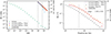 |
Fig. 12. Cumulative distribution of the S/Ns and fluences of FRBs in the SFR model. On the right ordinates, the number N detectable/detected for CHIME. On the left ordinate, the fraction of this number over the total, |

Our simulations indicate that equally bright FRB sources must next also be detectable in the side-lobes more often than the reported < 1% (3 out of 474). We expect a side-lobe detection fraction of ∼1.8% in the delayed SFR models, ∼2.2% in the straight SFR model, and ∼2.6% in the Euclidean model. The location of these detections are shown in Fig. 11. All the models considered here thus predict more side-lobe FRBs than Catalog 1 contains. This prediction percentage is consist over a large number of simulations, but the currently observed percentage could of course be affected by the small number statistics.
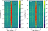 |
Fig. 11. Detection locations of simulated FRBs in the CHIME beam map (at 600 MHz). The left and right panels are results of the Euclidean and SFR number density model respectively. The vertical dashed lines mark the chosen boundary (±2.0°) of the main-lobe. Side-lobe detections account for ∼2.6% and ∼2.2% in the Euclidean and SFR models respectively, based on the average of 50 realizations. The beam intensity is normalized as in Fig. 3. |
An alternative explanation for both absences is that there is some intrinsic fluence cut off, which prevents side-lobe detections and high-S/N main-lobe detection alike. We note here that this required fluence cut-off differs from a cut-off or change in the luminosity function. The latter is of course possible, and occurs at the emission point, where the luminosity is defined. The fluence, however, is a value that is only defined at the observer location. As it is determined by a combination of the distance to the source and its luminosity, which are different for every FRB, the existence of such a cutoff seems very unlikely. The more likely explanation appears to be that there is a bias against high-S/N detections, and that some side-lobe detections go unrecognized as such.
5.5. The CHIME sensitivity and its influence on the S/N and fluence distribution
As introduced in Sect. 2.3.2, the initially predicted CHIME gain G = 1.4 K Jy−1, system temperature Tsys = 50 K and degradation factor β = 1.2 suggested in CHIME/FRB Collaboration (2018) and used in Gardenier et al. (2019) are found by the subsequent system study (Merryfield et al. 2023) to overestimate the CHIME/FRB sensitivity. Therefore, in this work, we adopted G = 1.0 K Jy−1, Tsys = 55 K, and β = 1.6 to agree with that study. These three parameters are most informatively combined when expressed as an effective system equivalent flux density SEFDeff = Tsysβ/G (see Eq. (10)). Thus, while frbpoppy previously assumed SEFDeff = 45 Jy, we now use SEFDeff = 90 Jy. This more realistic value underlies all above-mentioned results.
We here discuss the influence of this change on some of our metrics, especially on the agreement of the observed and simulated S/N distributions (see, e.g., Eq. (12)). In earlier sections, we have displayed these distributions as CDFs (e.g., Fig. 10). In this current discussion, we display similar data but now as distributions of cumulative number N(> x) versus x. Observed sets of bursts, for both one-offs and repeaters, are commonly visualized this way for either the number N(> x) or rate R(> x), against S/N, fluence or luminosity as variable x (e.g., CHIME/FRB Collaboration 2020b; Pastor-Marazuela et al. 2024).
We find that the change in SEFDeff has no influence on the slope and GoF of the S/N distribution. This indicates that despite selection effects and different telescope sensitivities, the S/N distribution remains scale-invariant. In Fig. 12 (left) this is visible from the identical sets of points for the two surveyed sets. In the same figure, the scale invariance is even more visible in the underlying S/N distribution (where we used SEFDeff∼ 90 Jy but no lower limit). The intrinsic population keeps a constant slope across almost the entire S/N range, thus validating the scale invariance of the S/N distribution. For comparison, the CHIME/FRB Catalog 1 sample is shown with star markers. It diverges from our trend from S/N > 50, suggesting CHIME missed high S/N events.
While the S/N distribution cannot distinguish between the old SEFDeff and the new, the fluence distribution can. As shown in Fig. 12 (right) the surveyed population with the updated G = 1.0 K Jy−1, β = 1.6 and Tsys = 55 K matches perfectly with the CHIME one-offs, while the survey using the preliminary, more sensitive value has significant discrepancies. For example, 38% of FRBs in the CHIME/FRB Catalog 1 have fluences > 5 Jy ms (the dashed line in the right panel of Fig. 12). The new SEFDeff recreates this very well (36%) where the old one could not (17%). We are thus confident the degradation factor is made up of actually occurring (and normal) imperfections or inefficiencies in the survey, related to e.g., corrections for the beam intensities, or pipelines.
5.6. Luminosity
In the current study, the lower and upper boundary of the luminosity are no longer free parameters as these are hard to constrain in the MCMC simulation. However, the Lmax can influence the maximum S/N in the surveyed population. Continuing the discussion from the previous subsections, the S/N threshold of CHIME/FRB Catalog 1 is 9 and the current maximum S/N is 132, which means the S/N range is smaller than two orders of magnitude. However, our luminosity range spans five orders of magnitude (1041–1046 erg s−1). Under the power-law distribution of luminosity, we would have expected 2%, i.e., of order 10, of the discovered FRBs to exceed this current maximum detected S/N of 132 (see Fig. 10, top panel). Of the detected sample, 0.1% of FRBs should have S/Ns > 1000; Given that the CHIME/FRB Catalog 1 contains ∼500 FRBs, the non-detection of such a burst is not constraining.
An exponential cutoff power distribution or smaller Lmax may result in a smaller maximum S/N in the simulated sample, although the proximity of the sources is unaffected, which is arguable more influential for this maximum S/N. We thus still expect that many large-S/N FRBs are observed when the sample size grows. The maximum S/N can provide an important clue on the luminosity distribution (e.g., a power-law or cutoff power-law, the Lmax or Lcutoff).
Below, we compared our results for the best-fit FRB luminosity models to other observational and theoretical results. While we discuss these, it is important to reiterate that two different definitions of the power-law index are commonly used, and care should be taken when comparing the results.
The luminosity power-law index li in frbpoppy is applied as dN(L)/d log L ∝ Lli or dN(L)/dL ∝ Lli − 1. Under this definition, integration reproduces li as the index in the cumulative distribution N(> L)∝Lli of the generated population. The other common definition is to report the exponent α from above-mentioned dN(L)/dL ∝ Lα, as reported in e.g., CHIME/FRB Collaboration (2020b). Thus, α = li − 1. Both are generally negative numbers. So an li = −1 is identical to α = −2. The index that determines the faint-end slope in the Schechter luminosity function is defined as this same α (Schechter 1976). Our li is this α plus one.
Now, our li could be measured directly as the slope in the log-log plot of N(> L) versus L of the intrinsic generated population. Selection effects, of course, alter this slope for the observed cosmological population of one-off bursts. This is displayed in Fig. 13: from an intrinsic population following li = −1.58, few bursts with L = 1043 erg s−1 are detected (the curve flattens toward lower Lbol). Brighter sources dominate the detected sample, meaning the population CHIME sees follows the much shallower power-law with index −0.75 ± 0.02. But for observations of repeater bursts, where fewer such effects occur, this li can be directly compared to the fits (e.g., Fig. 4 in Oostrum et al. 2020 or Fig. 3 in Kirsten et al. 2024).
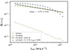 |
Fig. 13. Fractional cumulative number distribution of FRB luminosities, |

The preferred value for the luminosity index is  (Table 1). That is interesting, because this value based on one-off FRBs agrees with the value found by Oostrum et al. (2020, there called γ) for the repeating FRB 121102, of −1.7(6). It is also consistent with the most complete, high-fluence section of the broken power-law fit to luminosity index for repeating FRB 20180916B reported as −1.4 ± 0.1 in Pastor-Marazuela et al. (2021, there called Γ). This similarity in the pulse energy distribution between one-off and repeating FRBs, something that would be unlikely to occur between completely difference sources classes, corroborates the finding of Gardenier et al. (2021), recently confirmed by James (2023), that the two apparent types both originate from a single population of FRB sources that is actually mostly uniform.
A number of other studies of one-off populations, in contrast, find different values for the luminosity index, but there are important differences and caveats. We describe those below.
The study in Luo et al. (2020), while possibly limited by the small sample size, is similar in set up to frbpoppy, albeit without simulating cosmological source evolution. Luo et al. (2020) assumed a Schechter luminosity function and a log-normal intrinsic pulse width distribution, next applying a flux threshold Smin when calculating the joint likelihood function. Their best-fit model based on 46 FRBs from 7 surveys is formed by a Schechter luminosity index α of  with cutoff luminosity ∼3 × 1044 erg s−1. This index, which corresponds to our
 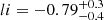 , governs the faint end of the N(> L) distribution, up to the turn-over luminosity. As FRBs with luminosities below L = 1043 erg s−1 do not significantly contribute to the observed population (see Fig. 13), the value of the index is not actually constraining. It is the turn-over itself that determines the distribution. To illustrate this behavior Fig. 13 also displays the resulting surveyed population, from a one-off experiment with a Schechter function in frbpoppy. Although the distribution is less linear, the Luo et al. (2020) result is similar to our best model in overall average slope.
Shin et al. (2023) next report a Schechter index α (called the differential power-law index there) of  , which in our notation corresponds to
  – but for the energy, not the luminosity. That result, too, is based on CHIME/FRB Catalog 1 data. The modeling, however, is more limited. Where frbpoppy finds the best model by fitting over the S/N, weff and DMtotal distributions, Shin et al. (2023) optimizes for the DMtotal–Fluence distributions. Fluence may be closely related to the luminosity index we discuss here, but it can only be turned into S/N, the observed quantity, through the pulse width. In Shin et al. (2023) this width is drawn from the inferred observed width distribution, not from an independent source distribution. To ensure understanding of the interplay between pulse width, luminosity and energy, forward modeling of the intrinsic pulse width and any broadening effects from the intervening plasma have been part of frbpoppy since inception (Gardenier et al. 2019). One of the main conclusions in Merryfield et al. (2023), too, is that the CHIME S/N is affected much more strongly by the effective burst width than by the DM. As the pulse widths are not explicitly modeled in Shin et al. (2023), the use of a single energy distribution, not separate luminosity and width distributions, is required. A number of inherent selection effects due to width may be absorbed into the energy function. We hence do not think a meaningful discussion of the astrophysics implied by our different luminosity and energy results is possible.
James et al. (2022a) find that the luminosity index dominates the extent to which FRBs are seen from the local universe, as suggested earlier by Macquart & Ekers (2018) – with steeper values indicating more nearby events in the observations. Therefore, the differences in the required li reflect the different FRB z distribution: James et al. (2022a) find 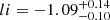 and in this case, the fraction of FRBs in the observed sample with z < 0.1 is ∼10%; while in our best model, the more negative li = −1.58 requires a larger fraction of local FRBs in the surveyed sample, of ∼50% below z = 0.1.
5.7. Pulse width
The log-normal distribution of intrinsic pulse width is inspired by those observed in pulsars and repeater pulses (Gardenier et al. 2019). It can naturally produce bursts from microseconds to a few seconds FRB duration, and cover at least six orders of magnitude, which is hard to achieve with a normal distribution. The best-fitting values for the pulse width distributions are constrained in our MCMC simulation and are consistent among different models: wint, mean ≃ 0.3 ms and wint, std ≃ 2 ms (Table 1). The result is a relatively broad best-fit input width distribution (Fig. 14, left panel). Bursts with larger intrinsic widths are also the higher fluence bursts. That is why the high-width tail is preferentially detected. Still, the pulse width contours in e.g., Fig. 7 are relatively well localized, indicating high confidence that this distribution shape is preferred. The slight correlation visible in the wint, mean–wint, std projection in that figure, showing that larger widths are required at higher means, indicates that generation of the sub-millisecond side is important.
The scattering time follows a log-normal distribution, as is visible in Fig. 14 (right panel). We compare our simulation outcomes against the boxcar width (bc width) provided in the CHIME/FRB Catalog 1, which takes an integer multiple of the 0.98304 ms time resolution. For FRBs of small intrinsic pulse width wint, the effective pulse width weff is dominated by tscat, tdm or tsamp. Fig. 14 shows that although there are many events with wint below 1 ms, all of the weff are above 1 ms due to the scattering and instrumental broadening around 600 MHz. We note that for many FRBs, the CHIME/FRB Catalog 1 only provides their tscat upper limits, which may cause a bias in modeling the lower end of wint.
We see here how two opposing selection effects are at play. In contrast to other models, that are energy based (and thus work in units of ergs; see James et al. 2022b), our model is luminosity based (e.g., working in units of erg s−1). This prevents simulations in which unphysically large amounts of energy are output per time unit. Some FRBs are as short as 10−6 s (see, e.g., Snelders et al. 2023, and note in Fig. 14 that these are indeed created in frbpoppy), others as bright as 1042 erg (Ryder et al. 2023); allowing a model to combine these would result in luminosities over 1048 erg s−1. Such a luminosity exceeds the maximum theoretical FRB luminosity under the assumptions of Lu & Kumar (2019), and the maximum spectral luminosities allowed in all but the most extreme parameter combinations in the models of Cooper & Wijers (2021). As described in Sect. 2.2.4, the top end of our luminosity range is based on the brightest observed FRBs; as these are harder to miss, this end is likely reasonably complete.
This luminosity basis of our model means wider pulses, on the one hand, have larger fluence (Eq. (8)) but on the other are somewhat harder to detect over the noise (Eq. (10)). Our treatment of these two selection effects allows us to reproduce the CHIME detected widths well. The higher-frequency surveys we next plan to include in frbpoppy alongside CHIME/FRB (see Sect. 2.2.3) suffer less from scattering effects, and more directly sample the narrower bursts (as evidenced in e.g. Pastor-Marazuela et al. 2024).
5.8. Dispersion by the baryonic IGM
The DMIGM, slope is relatively poorly constrained in the Euclidean and delayed SFR models, compared to the pure SFR model. This is expected as the fraction of low-z FRBs (e.g., z < 0.1) in the former models is higher than in the SFR model. The DMIGM, slope appears in the DMtotal as DMIGM, slopez. Therefore, to constrain DMIGM, slope better, more high redshift FRBs are needed. Within the 1σ uncertainty, the best-fitting values of DMIGM, slope are still consistent with the Macquart relation (Macquart et al. 2019; James et al. 2022a,b).
5.9. Host dispersion measures
One of the challenges in understanding the FRB population is that many of its intrinsic properties are tangled into only a small number of observed distributions. One such example is the interplay and overlap of the amount of dispersion caused by the host (DMhost), the density of the IGM (DMIGM, slope), and the distances to the sources. The first two are mainly constrained by the DMtotal and the weff distribution; while the distances are constrained by the DMtotal and the S/N distribution. There is an anti-correlation between DMIGM, slope and DMhost in the MCMC contour plot, most obvious in Fig. 7.
In our simulation, we allowed a DMhost (including the source contribution) to range over a log-normal distribution. That distribution is, at the moment, independent of the redshift. Contained in it are the possible inclination angles, and host galaxy types, averaging over their evolution between z = 1.5 and now. Figure 15 and Table 1 indicate that the best-fitting values of DMhost vary only slight between the different models. In Table 1 we list the mean values we find; our median DMhost in the source rest frame is ∼250 pc cm−3 for the SFR model and ∼340 pc cm−3 for Euclidean model respectively.
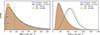 |
Fig. 15. Probability distribution of DMhost (left) in the source frame, and DMtotal (right) before (intrinsic) and after (surveyed) detection in our simulation. The median DMhost found by GL21, Shin et al. (2023) and this work are indicated with vertical dashed lines. The y axes are in linear scale. |
Our values are higher than assumed earlier (including in GL21, who find a constant value of 50 pc cm−3 produced an optimal fit). Our new results are also different from, e.g., Shin et al. (2023), who find a median DMhost of  pc cm−3 with a standard deviation of
  pc cm−3. The difference could, given the anti-correlation mentioned above, be caused by the value DMIGM, slope chosen in Shin et al. (2023), where it is not a free parameter. But we infer its value to be around 850 pc cm−3 (from their Fig. 10), not that different from our lowest result from the Euclidean model of DMIGM, slope ≃ 780 pc cm−3.
Both GL21 and Shin et al. (2023) find median DMhost values lower than the median DM of the known radio pulsars in our own Milky Way (where large selection effects against high-DM pulsar detection are at play, see e.g., van Leeuwen & Stappers 2010). As FRBs need to escape their host galaxy, which is often massive, it seems surprising it is found to be this low. We find median DMhost values of ∼300 pc cm−3 though, larger than the median for pulsars. In our results, the total DM is roughly comprised of equal contributions from DMhost and DMIGM, but higher values of DMtotal are generally driven by high host contributions, as visible in Fig. 10 (bottom panel). The median DM for the 6 radio magnetars in our Milky Way, however, is 700 pc cm−3. Our median DMhost values are starting to approach this value. In our Milky Way, the line of sight to magnetars cuts through the dense plane. Galaxies containing FRB-emitting magnetars (see CHIME/FRB Collaboration 2020a; Maan et al. 2022), on the other hand, are generally seen at an angle, with slightly lower DM. We conclude our results support a magnetar origin for FRBs.
The observed DMtotal distribution is a convolution of multiple components, many of which evolve over our sampled redshift range. The source DM contributions may vary strongly depending on the local conditions (supernova remnants, HII regions). The galaxy inclination angles matter for lower-redshift disk galaxies, and the distribution is an average over all these angles. Together, these sum to a DMhost distribution as shown in Fig. 15. This distribution can next be compared to the predictions from galaxy formation models (e.g., Jahns-Schindler et al. 2023) and cosmological simulations (for example, Orr et al. 2024).
From an overall model perspective, the main difference between our work and Shin et al. (2023) is that the latter authors find that the Pobs(z) distribution peaks at ∼0.36. None of the number density models that we consider (Power-law density, SFR or delayed SFR) produce a peak at such high redshift. Indeed, the differences in these redshift distributions are strongly correlated with the different DMhost between Shin et al. (2023) and our work. If the FRBs are located at higher z, a low DMhost is required to reproduce the observed DM curve. We find our values for DMhost are reasonable given the knowledge of the known host galaxies (e.g., Bhandari et al. 2022). As frbpoppy is open source, we encourage researchers to reproduce these results for themselves.
Our results indicate the selection effects against high-DM hosts are not very strong. This suggests FRBs from the centers of host galaxies are not strongly disfavored compared to those from the outskirts. That is interesting because sources such as magnetars or other young stellar remnants may be found closer to the center, where the dispersion is higher (see, e.g., van Leeuwen et al. 2020 for such a DM model), while globular cluster sources are found more at or beyond the host edge, where DMhost is lower.
5.10. Statistics
We use two statistical tools in this study. We employ the GoF to determine the global optimum parameters within a model, and we use the BIC method to choose between models, and determine which is the best. When deriving the log-likelihood function for the GoF, we have assumed the non-correlation of the three distributions. Although this does not strictly need to be the case, we find that when the minimum of ATotal2 is reached, the AS/N2, Aweff2 and ADM2 are all close to minimum as is shown in Table 2. We hence obtain the best-fitting values for all parameters simultaneously.
One could argue that for comparing between models, the Bayes factor is an even better tool, when considering the model complexity. Calculating the model evidence is, however, not included9 in the MCMC package emcee that is the main focus of the current study. We may consider Bayes factor comparison in future work. The BIC is sufficient for the problem at hand. We produced 50 surveyed populations for each model using the best-fitting parameters, and calculate BICs from the averaged GoFs to reduce the randomness. The results are shown in Table 2. The three delayed SFR models have very close BICs and cannot be distinguished from each other. They show a hint of evidence over the normal SFR model, but strong evidence over the Euclidean model.
5.11. Comparison with other studies
In Table 1 we compare the best-fitting values from our current work against those reported in GL21. In that study, frbpoppy could not yet produce formal errors; below, we estimate these from the width of the distributions plotted in Fig. 3 of GL21. Our value for α,  falls within the Cycle 1 range of the GL21 MC simulation, but in the following runs, their value moved away, to −2.2. Possibly our full MCMC approach is better able to find the correct global best fit. Our values for the power-law index are consistent with their near-flat li distribution.
Several reasons may account for the differences. In the current work, the parameters si, Lmin and Lmax are fixed instead of free. Furthermore, in GL21, the observed sample size is smaller, and not uniform in its selection effects. Next, the A-D test we now use for the GoF emphasizes other difference between distributions than the K–S test did. Finally, for finding the global maximum, the current MCMC implementation is a fundamental improvement over the GL21 MC simulation that ran multiple cycles over a number of parameter subsets.
James et al. (2022a,b) studied the z–DM distribution using the ASKAP and Parkes samples (with their code zDM10), by fitting over a DM-=redshift distribution model, a power-law energy distribution and a number density that evolves with modified SFR. They find an estimated maximum FRB energy of  (assuming a 1 GHz bandwidth), a cumulative luminosity index of
  (discussed previously), an SFR scaling parameter
  and a log-normal distribution of DMhost with mean
  pc cm−3.
Shin et al. (2023) build on James et al. (2022b), but now for CHIME/FRB Catalog 1. They performed a seven parameter MCMC inference based on the DM−Fluence distribution, in which the likelihood function was evaluated by comparing the counts per bin between the observed and modeled FRB samples. We contrasted their findings to ours in Sect. 5.9, specifically on the DM, the underlying number density input model, and the derived redshift distribution. We note that unlike James et al. (2022b), Shin et al. (2023) appear to not forward model the intrinsic pulse widths, or the subsequent scatter broadening. The authors use selection-corrected fiducial distributions from the injection system instead. This pulse width has a large, correlated influence on both the source and the telescope behavior. It strongly affects the telescope S/N, which is the most important metric for detection; and it has large influence on the emitted burst energy, assuming a given luminosity. Given these unmodeled correlations, Shin et al. (2023) necessarily have to limit their sample to avoid parts of the distribution where these selection effects occur. In the end, their comparison is based on 225 bursts. We model more selection effects, incorporate the entire catalog, and fit for more observables: S/N, weff and DMtotal.
Cui et al. (2022) selected a sample of 125 apparently non-repeating FRBs and report their luminosities follow a log-normal distribution. We, however, find a power-law luminosity function is a good fit. Possibly the selection criteria used in Cui et al. (2022), S/N > 12, introduces a bias against low luminosity FRBs and consequently add weight to the log-normal model.
Bhattacharyya et al. (2022) performed a three-parameter MCMC simulation with an 82 one-off burst sample to study the FRB spectral index, luminosity spectral index and mean energy. and Bhattacharyya et al. (2023) next used the CHIME/FRB Catalog 1 to perform a similar study. We have discussed in Sect. 2.2.3 that a survey at a single frequency is incapable of pinning down the spectral index, and allowing it to vary anyway introduces strong covariances in the luminosity function. This is prominent in the results reported in Bhattacharyya et al. (2023). We did not consider a Schechter luminosity function in our MCMC, and thus cannot compare against the cutoff energy and exponent found in Bhattacharyya et al. (2022). As the fitting of the energy distribution in that work does not appear to account for the selection function of the telescope, a meaningful comparison would have been difficult, regardless.
Chawla et al. (2022) studied the dispersion and scattering properties of the FRBs in Catalog 1, through a cosmological population synthesis. They find a DM distribution similar to ours, but their scattering time distribution that extends further into the high end (> 10 ms) than our results. Still, our pulse width distribution reproduces the widths seen by CHIME without the need of such a high-end tail. In the left-hand subplot of Fig. 14 this is visible from the agreement between the gray histogram and the green line. In that figure, the detected simulated pulses (orange) are clearly be part of the large-width tail of the intrinsic distribution (blue). Scattering, next, is a large further addition to the observed pulse width, as visible in the right sub-panel of Fig. 14.
Overall, we find that our results are based on matching more observables than other work and we consider them more robust. The validity of our best models is evidenced by the smaller error budgets we attain. For example, on the luminosity index we produce errors of −0.18, +0.10, significantly better than the −0.4, +0.7 of Shin et al. (2023) or the −0.4, +0.3 of Luo et al. (2020).
5.12. Snapshot data and result reproducibility
We provide a number of ways for interested astronomers to use our results. We discuss these below.
5.12.1. Model outcome packages
To get started immediately, one can navigate to the frbpoppy quickstart section on Zenodo11 and download 1_Day_FRB_Sky_on_Earth.txt. That human- and machine-readable file contains a simulated 1-day catalog of one-off FRBs, that allows users to access the FRB population without installing the entire frbpoppy package. Out of the 108.3 FRBs that happen every day between us and z = 1 (Sect. 5.1), 3.5 × 10⁶ are brighter than 0.01 Jy ms, the best limit in one-off FRB detection currently (Niu et al. 2021) and in the foreseeable future. The simulated catalog is produced by the perfect telescope in frbpoppy, free of selection effects, that observed 4π of sky for 24 h, with minimum detectable fluence 0.01 Jy ms, for the best-fit no-delay SFR model.
The catalog lists the coordinates, redshift, distance, width, DM, luminosity, fluence, and other properties for this 1-day snapshot of 3.5 × 10⁶ simulated detected one-off FRBs. Prospective users can integrate the accompanying python reader into their codes if they wish.
5.12.2. Open source code
Version 2.2.0 of frbpoppy is now available through GitHub12. The code continues to support all previous telescopes and population models (including repeating FRBs). This latest version includes the code optimizations and MCMC functionality described in Sect. 3.
5.13. Future work
Since frbpoppy now takes account into the selection effects important for CHIME/FRB, logical future steps include inferring the best-fitting populations from the next CHIME/FRB Catalog release. As frbpoppy is open source, any interested astronomer can take this on.
Furthermore, a more in-depth and direct comparison of the various population synthesis codes used in the community (mentioned in the previous section) would be of great interest if we want to understand code difference, and hence come to a more complete understanding of the actual population. Both frbpoppy and zDM (Prochaska et al. 2023) are open source, and we urge others to publish reproducibly, too.
Once available, such codes could be validated on the same data set as ground truth, with the same metrics. A collaboration that includes one of us started a similar benchmark for public FRB search codes (see Connor et al. 2020; Melo et al. 2020) with the goal of improving code and furthering open science. A similar comparison of population study codes would be beneficial for validation, improvement and sustainability of the projects involved.
The steady increase in the fractional bandwidth employed in FRB surveys may begin to warrant including in-band evolution of the FRB brightness and scatter broadening, as well as of the telescope sensitivity and beam pattern. For the current study we find those effects to be small enough, compared to other factors, to stay with the quasi-monochromatic approach. For tscat and tDM, for example, one could use weighted averages over the band. For our median DMtotal value of ∼550 pc cm−3 (e.g., Fig. 10) the weighted average over tscat is 0.3 ms larger than the central value we use now (see Eq. (13) in Gardenier et al. 2019). This is below the CHIME sampling time, and would not meaningfully influence the surveyed tscat distribution (a 0.2σ shift in Fig. 14). The effect on tDM is another factor of two smaller. It would be an improvement to include this in the future none the less, especially for searches with even lower frequency telescopes such as LOFAR and Square Kilometre Array (SKA)-Low (e.g., Coenen et al. 2014).
Natural progression of the current results (as mentioned before) could entail inclusion of Schechter, broken power-law, or log-normal distributions for the luminosity function, and of the Bayes factor for comparing models. Modeling of CHIME/FRB repeater FRBs, and the addition of the other new surveys with tens of FRB detections, would also be highly interesting.
6. Conclusions
The updated frbpoppy is able to perform an MCMC on the entire CHIME/FRB Catalog 1 and find a single best model for the birth and evolution of the real, underlying FRB population. Where other studies had to curate the input FRBs, our treatment of selection effects allows us to use all one-off FRBs, producing better fits, with smaller errors, than before.
Every Earth day ∼2 × 10⁸ FRBs go off between us and z = 1, and we make available the mock catalog of the 3.5 × 10⁶ that are potentially detectable. Some of these are nearby and very bright, and we have presented evidence that a number of these were missed by CHIME/FRB.
We show that contributions to the DM by the host of several 100s of pc cm−3 best describe the observed dispersion distribution. We thus conclude selection effects against relatively high-DM hosts are not very strong.
We find strong evidence that the FRB population evolves with look-back time, following star formation, with a slight preference for a small delay. We conclude FRBs are produced by the remnants of short-lived stars. The results from our combination of the largest, single-survey data set and the most comprehensive population synthesis code available at the moment thus lend population-based support to the hypothesis that FRBs are created by neutron stars.
Data availability
The code and models used here are available at https://github.com/TRASAL/frbpoppy. A snapshot 1-day catalog is available at https://doi.org/10.5281/zenodo.11091637
FRB POPulation synthesis in PYthon; https://github.com/TRASAL/frbpoppy
In frbpoppy the catalog is obtained from the Transient Name Server (TNS), through a query on these dates.
The Hubble-Lemaître tension (Riess et al. 2022; Hu & Wang 2023) between the local distance indicator and the cosmic microwave background (CMB) can result in up to 10% discrepancy in distances and the inferred redshifts from DMIGM. The impact of this uncertainty is not investigated in this work.
Called si in GL21.
Using the python module emcee (Foreman-Mackey et al. 2013), https://github.com/dfm/emcee
For S/N, we compare with bonsai_snr in CHIME/FRB Catalog 1.
https://www.surf.nl/en/dutch-national-supercomputer-snellius
Acknowledgments
We thank David Gardenier, Leon Oostrum, and Dany Vohl for interesting discussions and for their support, and Pikky Atri, Kaustubh Rajwade, Ralph Wijers and the anonymous referee for suggestions that improved this work. This research was supported by the following projects, all financed by the Dutch Research Council (NWO): Vici research project “ARGO” (grant number 639.043.815); CORTEX (NWA.1160.18.316), under the research programme NWA-ORC; plus EINF-3624 and EINF-7739 of the research programme “Computing Time on National Computing Facilities” hosted by SURF.
References
- Abbott, B. P., Abbott, R., Abbott, T. D., et al. 2017, Phys. Rev. Lett., 119, 161101 [Google Scholar]
- Amiri, M., Bandura, K., Boskovic, A., et al. 2022, ApJ, 932, 100 [NASA ADS] [CrossRef] [Google Scholar]
- Bates, S. D., Lorimer, D. R., Rane, A., & Swiggum, J. 2014, MNRAS, 439, 2893 [NASA ADS] [CrossRef] [Google Scholar]
- Bhandari, S., Heintz, K. E., Aggarwal, K., et al. 2022, AJ, 163, 69 [NASA ADS] [CrossRef] [Google Scholar]
- Bhardwaj, M., Gaensler, B. M., Kaspi, V. M., et al. 2021, ApJ, 910, L18 [NASA ADS] [CrossRef] [Google Scholar]
- Bhattacharyya, S., Tiwari, H., Bharadwaj, S., & Majumdar, S. 2022, MNRAS, 513, L1 [NASA ADS] [CrossRef] [Google Scholar]
- Bhattacharyya, S., Bharadwaj, S., Tiwari, H., & Majumdar, S. 2023, MNRAS, 522, 3349 [NASA ADS] [CrossRef] [Google Scholar]
- Bilous, A. V., van Leeuwen, J., Maan, Y., et al. 2024, A&A, submitted [arXiv: 2407.05366] [Google Scholar]
- Bochenek, C. D., Ravi, V., Belov, K. V., et al. 2020, Nature, 587, 59 [NASA ADS] [CrossRef] [Google Scholar]
- Burke-Spolaor, S., Bailes, M., Ekers, R., Macquart, J.-P., & Crawford, F. 2010, ApJ, 727, 18 [Google Scholar]
- Chawla, P., Kaspi, V. M., Ransom, S. M., et al. 2022, ApJ, 927, 35 [NASA ADS] [CrossRef] [Google Scholar]
- CHIME/FRB Collaboration (Amiri, M., et al.) 2018, ApJ, 863, 48 [NASA ADS] [CrossRef] [Google Scholar]
- CHIME/FRB Collaboration (Amiri, M., et al.) 2019, Nature, 566, 230 [NASA ADS] [CrossRef] [Google Scholar]
- CHIME/FRB Collaboration (Andersen, B. C., et al.) 2020a, Nature, 587, 54 [Google Scholar]
- CHIME/FRB Collaboration (Amiri, M., et al.) 2020b, Nature, 582, 351 [NASA ADS] [CrossRef] [Google Scholar]
- CHIME/FRB Collaboration (Amiri, M., et al.) 2021, ApJS, 257, 59 [NASA ADS] [CrossRef] [Google Scholar]
- Coenen, T., van Leeuwen, J., Hessels, J. W. T., et al. 2014, A&A, 570, A60 [NASA ADS] [CrossRef] [EDP Sciences] [Google Scholar]
- Connor, L. 2019, MNRAS, 487, 5753 [Google Scholar]
- Connor, L., van Leeuwen, J., Mendrik, A., et al. 2020, An Open-source, Open-participation Competition for Fast Radio Burst Detection, https://github.com/EYRA-Benchmark/frb-benchmark [Google Scholar]
- Cooper, A. J., & Wijers, R. A. M. J. 2021, MNRAS, 508, L32 [NASA ADS] [CrossRef] [Google Scholar]
- Cordes, J. M., & Chatterjee, S. 2019, ARA&A, 57, 417 [NASA ADS] [CrossRef] [Google Scholar]
- Cordes, J. M., & Lazio, T. J. W. 2002, ArXiv e-prints [arXiv:astro-ph/0207156] [Google Scholar]
- Cordes, J. M., & Lazio, T. J. W. 2003, ArXiv e-prints [arXiv:astro-ph/0301598] [Google Scholar]
- Cui, X.-H., Zhang, C.-M., Li, D., et al. 2022, Ap&SS, 367, 66 [NASA ADS] [CrossRef] [Google Scholar]
- Fong, W., Berger, E., Margutti, R., & Zauderer, B. A. 2015, ApJ, 815, 102 [NASA ADS] [CrossRef] [Google Scholar]
- Foreman-Mackey, D., Hogg, D. W., Lang, D., & Goodman, J. 2013, PASP, 125, 306 [Google Scholar]
- Gardenier, D. W. 2019, Astrophysics Source Code Library [record ascl:1911.009] [Google Scholar]
- Gardenier, D. W., & van Leeuwen, J. 2021, A&A, 651, A63 [NASA ADS] [CrossRef] [EDP Sciences] [Google Scholar]
- Gardenier, D. W., van Leeuwen, J., Connor, L., & Petroff, E. 2019, A&A, 632, A125 [NASA ADS] [CrossRef] [EDP Sciences] [Google Scholar]
- Gardenier, D. W., Connor, L., van Leeuwen, J., Oostrum, L. C., & Petroff, E. 2021, A&A, 647, A30 [EDP Sciences] [Google Scholar]
- Hu, J.-P., & Wang, F.-Y. 2023, Universe, 9, 94 [CrossRef] [Google Scholar]
- Jahns-Schindler, J. N., Spitler, L. G., Walker, C. R. H., & Baugh, C. M. 2023, MNRAS, 523, 5006 [NASA ADS] [CrossRef] [Google Scholar]
- James, C. W. 2023, PASA, 40, e057 [NASA ADS] [CrossRef] [Google Scholar]
- James, C. W., Ekers, R. D., Macquart, J. P., Bannister, K. W., & Shannon, R. M. 2019, MNRAS, 483, 1342 [NASA ADS] [CrossRef] [Google Scholar]
- James, C. W., Prochaska, J. X., Macquart, J. P., et al. 2022a, MNRAS, 510, L18 [Google Scholar]
- James, C. W., Prochaska, J. X., Macquart, J. P., et al. 2022b, MNRAS, 509, 4775 [Google Scholar]
- Keane, E. F., & Kramer, M. 2008, MNRAS, 391, 2009 [Google Scholar]
- Kirsten, F., Marcote, B., Nimmo, K., et al. 2022, Nature, 602, 585 [NASA ADS] [CrossRef] [Google Scholar]
- Kirsten, F., Ould-Boukattine, O. S., Herrmann, W., et al. 2024, Nat. Astron., 8, 337 [NASA ADS] [CrossRef] [Google Scholar]
- Kremer, K., Fuller, J., Piro, A. L., & Ransom, S. M. 2023, MNRAS, 525, L22 [NASA ADS] [CrossRef] [Google Scholar]
- Lazarus, P., Kaspi, V. M., Champion, D. J., Hessels, J. W. T., & Dib, R. 2012, ApJ, 744, 97 [NASA ADS] [CrossRef] [Google Scholar]
- Lin, H. H., Scholz, P., Ng, C., et al. 2023, ArXiv e-prints [arXiv:2307.05262] [Google Scholar]
- Lorimer, D. R., & Kramer, M. 2004, Handbook of Pulsar Astronomy, 4 [Google Scholar]
- Lorimer, D. R., Bailes, M., McLaughlin, M. A., Narkevic, D. J., & Crawford, F. 2007, Science, 318, 777 [Google Scholar]
- Lorimer, D. R., Karastergiou, A., McLaughlin, M. A., & Johnston, S. 2013, MNRAS, 436, L5 [NASA ADS] [CrossRef] [Google Scholar]
- Lu, W., & Kumar, P. 2019, MNRAS, 483, L93 [CrossRef] [Google Scholar]
- Luo, R., Men, Y., Lee, K., et al. 2020, MNRAS, 494, 665 [NASA ADS] [CrossRef] [Google Scholar]
- Maan, Y., van Leeuwen, J., Straal, S., & Pastor-Marazuela, I. 2022, ATel, 15697, 1 [NASA ADS] [Google Scholar]
- Macquart, J. P., & Ekers, R. 2018, MNRAS, 480, 4211 [NASA ADS] [CrossRef] [Google Scholar]
- Macquart, J. P., Shannon, R. M., Bannister, K. W., et al. 2019, ApJ, 872, L19 [NASA ADS] [CrossRef] [Google Scholar]
- Macquart, J. P., Prochaska, J. X., McQuinn, M., et al. 2020, Nature, 581, 391 [Google Scholar]
- Mannings, A. G., Fong, W.-F., Simha, S., et al. 2021, ApJ, 917, 75 [NASA ADS] [CrossRef] [Google Scholar]
- Melinder, J., Dahlen, T., Mencía Trinchant, L., et al. 2012, A&A, 545, A96 [NASA ADS] [CrossRef] [EDP Sciences] [Google Scholar]
- Melo, A., Rubbert, S., Akhmerov, A., et al. 2020, https://doi.org/10.5281/zenodo.3903257 [Google Scholar]
- Merryfield, M., Tendulkar, S. P., Shin, K., et al. 2023, AJ, 165, 152 [NASA ADS] [CrossRef] [Google Scholar]
- Mikhailov, K., & van Leeuwen, J. 2016, A&A, 593, A21 [NASA ADS] [CrossRef] [EDP Sciences] [Google Scholar]
- Mo, J.-F., Zhu, W., Wang, Y., Tang, L., & Feng, L.-L. 2023, MNRAS, 518, 539 [Google Scholar]
- Nicholl, M., Williams, P. K. G., Berger, E., et al. 2017, ApJ, 843, 84 [NASA ADS] [CrossRef] [Google Scholar]
- Niu, C.-H., Li, D., Luo, R., et al. 2021, ApJ, 909, L8 [NASA ADS] [CrossRef] [Google Scholar]
- Oostrum, L. C., Maan, Y., van Leeuwen, J., et al. 2020, A&A, 635, A61 [NASA ADS] [CrossRef] [EDP Sciences] [Google Scholar]
- Oppermann, N., Connor, L. D., & Pen, U.-L. 2016, MNRAS, 461, 984 [NASA ADS] [CrossRef] [Google Scholar]
- Orr, M. E., Burkhart, B., Lu, W., Ponnada, S. B., & Hummels, C. B. 2024, ApJ, submitted [arXiv:2406.03523] [Google Scholar]
- Pastor-Marazuela, I., Connor, L., van Leeuwen, J., et al. 2021, Nature, 596, 505 [NASA ADS] [CrossRef] [Google Scholar]
- Pastor-Marazuela, I., van Leeuwen, J., Bilous, A., et al. 2024, A&A, submitted [arXiv:2406.00482] [Google Scholar]
- Petroff, E., Keane, E. F., Barr, E. D., et al. 2015, MNRAS, 451, 3933 [NASA ADS] [CrossRef] [Google Scholar]
- Petroff, E., Hessels, J. W. T., & Lorimer, D. R. 2019, A&A Rev., 27, 4 [NASA ADS] [CrossRef] [Google Scholar]
- Petroff, E., Hessels, J. W. T., & Lorimer, D. R. 2022, A&A Rev., 30, 2 [NASA ADS] [CrossRef] [Google Scholar]
- Planck Collaboration XIII. 2016, A&A, 594, A13 [NASA ADS] [CrossRef] [EDP Sciences] [Google Scholar]
- Pol, N., McLaughlin, M., & Lorimer, D. R. 2019, ApJ, 870, 71 [NASA ADS] [CrossRef] [Google Scholar]
- Prochaska, J. X., & Zheng, Y. 2019, MNRAS, 485, 648 [NASA ADS] [Google Scholar]
- Prochaska, J. X., Baptista, J., Ghosh, E. M., & James, C. W. 2023, https://zenodo.org/records/8192369 [Google Scholar]
- Raftery, A. E. 1995, Sociol. Methodol., 25, 111 [CrossRef] [Google Scholar]
- Rajwade, K. M., & van Leeuwen, J. 2024, Universe, 10, 158 [NASA ADS] [CrossRef] [Google Scholar]
- Ravi, V. 2019, Nat. Astron., 3, 928 [NASA ADS] [CrossRef] [Google Scholar]
- Riess, A. G., Yuan, W., Macri, L. M., et al. 2022, ApJ, 934, L7 [NASA ADS] [CrossRef] [Google Scholar]
- Ryder, S. D., Bannister, K. W., Bhandari, S., et al. 2023, Science, 382, 294 [NASA ADS] [CrossRef] [Google Scholar]
- Schechter, P. 1976, ApJ, 203, 297 [Google Scholar]
- Scholz, F. W., & Stephens, M. A. 1987, J. Am. Stat. Assoc., 918 [Google Scholar]
- Shannon, R. M., Macquart, J. P., Bannister, K. W., et al. 2018, Nature, 562, 386 [NASA ADS] [CrossRef] [Google Scholar]
- Shin, K., Masui, K. W., Bhardwaj, M., et al. 2023, ApJ, 944, 105 [NASA ADS] [CrossRef] [Google Scholar]
- Snelders, M. P., Nimmo, K., Hessels, J. W. T., et al. 2023, Nat. Astron., 7, 1486 [NASA ADS] [CrossRef] [Google Scholar]
- Straal, S. M., & van Leeuwen, J. 2019, A&A, 623, A90 [NASA ADS] [CrossRef] [EDP Sciences] [Google Scholar]
- Taylor, J. H., & Manchester, R. N. 1977, ApJ, 215, 885 [NASA ADS] [CrossRef] [Google Scholar]
- Thompson, C., & Duncan, R. C. 1995, MNRAS, 275, 255 [Google Scholar]
- Thornton, D., Stappers, B., Bailes, M., et al. 2013, Science, 341, 53 [NASA ADS] [CrossRef] [Google Scholar]
- van Leeuwen, J., & Stappers, B. W. 2010, A&A, 509, A7 [NASA ADS] [CrossRef] [EDP Sciences] [Google Scholar]
- van Leeuwen, J., & Verbunt, F. 2004, in Young Neutron Stars and Their Environments, eds. F. Camilo, & B. M. Gaensler, 218, 41 [NASA ADS] [Google Scholar]
- van Leeuwen, J., Mikhailov, K., Keane, E., et al. 2020, A&A, 634, A3 [NASA ADS] [CrossRef] [EDP Sciences] [Google Scholar]
- van Leeuwen, J., Kooistra, E., Oostrum, L., et al. 2023, A&A, 672, A117 [NASA ADS] [CrossRef] [EDP Sciences] [Google Scholar]
- Yamasaki, S., & Totani, T. 2020, ApJ, 888, 105 [NASA ADS] [CrossRef] [Google Scholar]
- Yang, Y.-P., Luo, R., Li, Z., & Zhang, B. 2017, ApJ, 839, L25 [Google Scholar]
- Zhang, B. 2018, ApJ, 867, L21 [NASA ADS] [CrossRef] [Google Scholar]
- Zhang, G. Q., Yu, H., He, J. H., & Wang, F. Y. 2020, ApJ, 900, 170 [NASA ADS] [CrossRef] [Google Scholar]
- Zhang, R. C., Zhang, B., Li, Y., & Lorimer, D. R. 2021, MNRAS, 501, 157 [Google Scholar]
- Zhang, R. C., & Zhang, B. 2022, ApJ, 924, L14 [NASA ADS] [CrossRef] [Google Scholar]
Appendix A: Summary of parameters and acronyms
The long form and meaning of the parameters and abbreviations used in this work.
All Tables
The long form and meaning of the parameters and abbreviations used in this work.
All Figures
|
Fig. 1. DM distribution histogram of one-off FRBs in the TNS database. The total sample of FRBs is shown in blue while those from CHIME/FRB and other telescopes are shown in orange and green respectively. |
| In the text | |
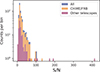 |
Fig. 2. S/N distribution histogram of one-off FRBs, using the same labels and colors as Fig. 1. |
| In the text | |
|
Fig. 14. Probability distribution of pulse width and broadening effects. Left panel: normalized distribution of intrinsic pulse width wint, for the intrinsic, generated sample and for the surveyed, detected sample, the effective pulse width weff of this surveyed sample in the simulation, and of the CHIME/FRB Catalog 1 widths. Right panel: distribution of the simulated normalized tdm and tscat subcomponents of the width of the surveyed, detected FRBs; compared to the values from the CHIME/FRB Catalog 1. The sampling time tsamp of 0.98304 ms is marked with a dashed line. The population is generated using best-fitting values for the 0.1-Gyr delayed SFR model. |
| In the text | |
|
Fig. 3. CHIME/FRB beam model reproduced with cfbm at 600 MHz. The left panel shows the beam intensity map in the range [ − 40° ,40° ] (East-West) and [ − 60° ,60° ] (North-South). The upper and bottom right panels show the East-West slice (y = 0°) and North-South slice along the meridian (x = 0°) respectively. The relative beam intensity is dimensionless, and normalized to the transit of Cyg A (Amiri et al. 2022). To include the side-lobe in our simulation, the beam range [ − 15° ,15° ] (East-West) × [−60° ,60° ] (North-South) is considered, where the East-West borders are indicated with dash-dotted lines. |
| In the text | |
|
Fig. 4. Three-dimensional GoF plot for {α, γ, li} from an MC simulation. Different GoFs are denoted with colors as well as marker sizes. |
| In the text | |
|
Fig. 5. Cumulative distribution plots of S/N, weff and DMtotal distributions from two surveyed populations generated with and without reuse, for the Euclidean model. The p-value of K–S test is also shown for reference. |
| In the text | |
|
Fig. 6. Confidence contours and marginalized likelihood distributions for the 7 parameters in our power-law number density model. |
| In the text | |
|
Fig. 7. Confidence contours and marginalized likelihood distributions for the 6 parameters in our SFR model. |
| In the text | |
|
Fig. 8. Probability distributions of FRBs as functions of redshift for different models. Left panel: probability density functions (PDFs) of the intrinsic FRB population versus redshift, for the Euclidean, SFR and delayed SFR models with three delay times. The redshift range [0, 1.5] is used in our simulation. For information, we also show the region [1.5, 2.5], gray shaded, such that the shift of the SFR peak is visible between the models. Right panel: simulated observed FRB population PDFs against redshift, for the same models. The mean redshift ⟨z⟩ for the different models are marked by the dashed vertical lines. An unfilled zoomed-in view of the redshift range [0, 0.2] is also shown. |
| In the text | |
|
Fig. 9. Confidence contours and marginalized likelihood distributions for three delayed SFR model (0.1, 0.5, 1.0 Gyr). |
| In the text | |
|
Fig. 10. Comparison of cumulative distributions for simulated populations with best-fitting parameters and the CHIME/FRB Catalog 1 one-off FRBs. The S/N, weff and DMtotal are shown in upper, middle and lower panels respectively. The population coloring is the same in all subplots. In the DM plot we also show the cumulative contributions of DMhost/(1 + z), and of the additional DMIGM, for the delayed SFR model with 0.1 Gyr. These show how, for the lower-DM half of the population, these two components contribute roughly equally to the DMtotal; while for the higher-DM half, the host contribution dominates. |
| In the text | |
|
Fig. 12. Cumulative distribution of the S/Ns and fluences of FRBs in the SFR model. On the right ordinates, the number N detectable/detected for CHIME. On the left ordinate, the fraction of this number over the total, |
| In the text | |
|
Fig. 11. Detection locations of simulated FRBs in the CHIME beam map (at 600 MHz). The left and right panels are results of the Euclidean and SFR number density model respectively. The vertical dashed lines mark the chosen boundary (±2.0°) of the main-lobe. Side-lobe detections account for ∼2.6% and ∼2.2% in the Euclidean and SFR models respectively, based on the average of 50 realizations. The beam intensity is normalized as in Fig. 3. |
| In the text | |
|
Fig. 13. Fractional cumulative number distribution of FRB luminosities, |
| In the text | |
|
Fig. 15. Probability distribution of DMhost (left) in the source frame, and DMtotal (right) before (intrinsic) and after (surveyed) detection in our simulation. The median DMhost found by GL21, Shin et al. (2023) and this work are indicated with vertical dashed lines. The y axes are in linear scale. |
| In the text | |
Current usage metrics show cumulative count of Article Views (full-text article views including HTML views, PDF and ePub downloads, according to the available data) and Abstracts Views on Vision4Press platform.
Data correspond to usage on the plateform after 2015. The current usage metrics is available 48-96 hours after online publication and is updated daily on week days.
Initial download of the metrics may take a while.