Ultraviolet H2 luminescence in molecular clouds induced by cosmic rays

Marco Padovani; Daniele Galli; Liam H. Scarlett; Tommaso Grassi; Una S. Rehill; Mark C. Zammit; Igor Bray; Dmitry V. Fursa

doi:10.1051/0004-6361/202348168

Home

All issues

Volume 682 (February 2024)

A&A, 682 (2024) A131

Full HTML

Open Access

Issue		A&A Volume 682, February 2024


Article Number		A131
Number of page(s)		22
Section		Interstellar and circumstellar matter
DOI		https://doi.org/10.1051/0004-6361/202348168
Published online		13 February 2024

A&A, 682, A131 (2024)

Ultraviolet H₂ luminescence in molecular clouds induced by cosmic rays

Marco Padovani¹, Daniele Galli¹, Liam H. Scarlett², Tommaso Grassi³, Una S. Rehill², Mark C. Zammit⁴, Igor Bray² and Dmitry V. Fursa²

¹ INAF – Osservatorio Astrofisico di Arcetri, Largo E. Fermi 5, 50125 Firenze, Italy
e-mail: marco.padovani@inaf.it
² Department of Physics and Astronomy, Curtin University, Perth, Western Australia 6102, Australia
³ Max-Planck-Institut für extraterrestrische Physik, Giessenbachstrasse 1, 85748 Garching, Germany
⁴ Theoretical Division, Los Alamos National Laboratory, Los Alamos, NM 87545, USA

Received: 5 October 2023
Accepted: 1 December 2023

Abstract

Context. Galactic cosmic rays (CRs) play a crucial role in ionisation, dissociation, and excitation processes within dense cloud regions where UV radiation is absorbed by dust grains and gas species. CRs regulate the abundance of ions and radicals, leading to the formation of more and more complex molecular species, and determine the charge distribution on dust grains. A quantitative analysis of these effects is essential for understanding the dynamical and chemical evolution of star-forming regions.

Aims. The CR-induced photon flux has a significant impact on the evolution of the dense molecular medium in its gas and dust components. This study evaluates the flux of UV photons generated by CRs to calculate the photon-induced dissociation and ionisation rates of a vast number of atomic and molecular species, as well as the integrated UV photon flux.

Methods. To achieve these goals, we took advantage of recent developments in the determination of the spectra of secondary electrons, in the calculation of state-resolved excitation cross sections of H₂ by electron impact, and of photodissociation and photoionisation cross sections.

Results. We calculated the H₂ level population of each rovibrational level of the X, B, C, B′, D, B″, D′, and a states. We then computed the UV photon spectrum of H₂ in its line and continuum components between 72 and 700 nm, with unprecedented accuracy, as a function of the CR spectrum incident on a molecular cloud, the H₂ column density, the isomeric H₂ composition, and the dust properties. The resulting photodissociation and photoionisation rates are, on average, lower than previous determinations by a factor of about 2, with deviations of up to a factor of 5 for the photodissociation of species such as AlH, C₂H₂, C₂H₃, C₃H₃, LiH, N₂, NaCl, NaH, O₂⁺, S₂, SiH, l-C₄, and l-C₅H. A special focus is given to the photoionisation rates of H₂, HF, and N₂, as well as to the photodissociation of H₂, which we find to be orders of magnitude higher than previous estimates. We give parameterisations for both the photorates and the integrated UV photon flux as a function of the CR ionisation rate, which implicitly depends on the H₂ column density, as well as the dust properties.

Key words: astrochemistry / atomic processes / molecular processes / cosmic rays / dust, extinction / ultraviolet: ISM

© The Authors 2024

Open Access article, published by EDP Sciences, under the terms of the Creative Commons Attribution License (https://creativecommons.org/licenses/by/4.0), which permits unrestricted use, distribution, and reproduction in any medium, provided the original work is properly cited.

This article is published in open access under the Subscribe to Open model. Subscribe to A&A to support open access publication.

1 Introduction

The interplay between cosmic-ray (CR) induced processes and the chemical evolution of molecular clouds is a crucial element in our understanding of the astrophysical environment. Such findings advance our comprehension of fundamental astrophys-ical phenomena and shed light on the interconnections between CR physics and astrochemistry. Galactic CRs can penetrate into the densest regions of molecular clouds, where ultraviolet (UV) radiation is blocked by the absorption of dust grains and molecular species. In these dark cloud regions, with H₂ column densities higher than about 3−4 × 10²¹ cm⁻², CRs dominate the processes of ionisation, dissociation, and excitation of gas species. The ionisation of H₂ is the main energy loss process of CRs in a molecular cloud, and a key element in the physical and chemical evolution of star-forming regions. The rate of ionisation of H₂ by CRs, ξH₂, is a fundamental parameter in non-ideal magnetohydrodynamic simulations and astrochemical models¹:

(i)
The ionisation fraction, which is a function of $ζ_{H_{2}}$ $${\zeta _{{{\rm{H}}_2}}}$ , controls the degree of coupling between the gas and the cloud’s magnetic field, influencing the collapse time of molecular clouds.
(ii)
Newly formed $H_{2}^{+}$ ${\rm{H}}_2^ +$ ions react immediately with other hydrogen molecules to form $H_{3}^{+}$ ${\rm{H}}_3^ +$ , starting a cascade of chemical reactions that lead to the formation of increasingly complex molecules, up to what are believed to be the building blocks of terrestrial life (Caselli & Ceccarelli 2012).
(iii)
The CR-induced dissociation of H₂ has important consequences for the formation of complex molecules, such as CH₃OH (Tielens & Hagen 1982) and NH₃ (Hiraoka et al. 1995; Fedoseev et al. 2015), on the grain surface through the process of hydrogenation.
(iv)
CR-excited rovibrational levels of the ground state of H₂ radiatively decay to the ground level, producing a flux of near-infrared (NIR) photons. Bialy (2020) developed a model, extended in Padovani et al. (2022) and tested observationally in Bialy et al. (2022) towards dark clouds, showing that from the NIR photon flux it is possible to estimate $ζ_{H_{2}}$ ${\zeta _{{{\rm{H}}_2}}}$ without having to resort to chemical networks and secondary species.
(v)
CR-excited electronic states of H₂ radiatively decay to rovibrational levels of the ground state, producing a UV photon flux, mostly in the Lyman-Werner bands, known as the Prasad-Tarafdar effect (Prasad & Tarafdar 1983). These UV photons have a dual effect: they extract electrons from dust grains via the photoelectric effect, significantly affecting the dust grain charge distribution, and they photodissociate and photoionise atomic and molecular species.

Prasad & Tarafdar (1983) first presented a quantitative method for estimating the UV emission in the Lyman-Werner bands of H₂ collisionally excited by CR particles. In their pioneering work, they considered a generic excited electronic level (to be interpreted as an appropriate combination of electronic, vibrational, and rotational levels) and a generic excited ground state level other than v = 0. Sternberg et al. (1987) evaluated the Lyman-Werner band emission of CR-excited H₂ and computed the resulting photodissociation rates of several interstellar molecules, focusing in particular on the effects of the CR-generated UV flux on the chemistry of H₂O and simple hydrocarbons. This work was extended by Gredel et al. (1987) (specifically to evaluate the CO/C ratio in molecular clouds) and Gredel et al. (1989), who included several excited electronic states of H₂ to evaluate photodissociation and photoionisation rates of a large set of molecules. The procedure followed by Gredel et al. (1989) is summarised in Appendix A.

Recent theoretical and observational developments in the study of the propagation of CRs in molecular clouds, of the production of secondary CR electrons, and the availability of state-resolved cross sections of H₂ excitation by electron impact make it possible to revise and update the results obtained in these studies. In particular, in this work we have taken the following developments into account:

(i)
CR propagation models have shown that the CR ionisa-tion rate decreases with H₂ column density, spanning a large range of orders of magnitude (10⁻¹⁴ − 10⁻¹⁸ s⁻¹) for column densities between 10²⁰ and 10²⁵ cm⁻², depending on the assumptions on the Galactic CR spectrum (see e.g. Padovani et al. 2009, 2018b, 2022). This has been supported by a vast number of observational estimates of ζH₂ obtained in different environments: in diffuse regions of molecular clouds (Shaw et al. 2008; Neufeld et al. 2010; Indriolo & McCall 2012; Neufeld & Wolfire 2017; Luo et al. 2023a,b), in low-mass pre-stellar cores (Caselli et al. 1998; Maret & Bergin 2007; Fuente et al. 2016; Redaelli et al. 2021; Bialy et al. 2022), in high-mass star-forming regions (de Boisanger et al. 1996; van der Tak et al. 2000; Hezareh et al. 2008; Morales Ortiz et al. 2014; Sabatini et al. 2020, 2023), in circumstellar discs (Ceccarelli et al. 2004), and in massive hot cores (Barger & Garrod 2020). We refer to Appendix B for an updated view of CR ionisation rate estimates from observations and their comparison with theoretical models.
(ii)
Thanks to the methodology recently developed by Ivlev et al. (2021), it is now possible to rigorously determine the energy spectrum of secondary electrons as a function of the column density for any proton spectrum incident on the cloud (see Sect. 3.1 and Padovani et al. 2022), eliminating the approximation of mono-energetic secondary electrons (usually assumed to have energy of about 30 eV; see e.g. Gredel & Dalgarno 1995).
(iii)
Finally, the accuracy of collisional excitation rates of H₂ has substantially increased thanks to the recent availability of molecular convergent close-coupling (MCCC) calculations (Scarlett et al. 2023), where vibrationally and rotationally resolved electron excitation cross sections of H₂ are computed for a large set of electronic states (see Sect. 2.4).

As a result of these improvements, we can compute the spectrum of CR-generated UV photons in the wavelength range between 72 and 700 nm with unprecedented accuracy. This allows us (i) to generate a new set of photodissociation and photoionisation rates of atomic and molecular species relevant to astrochemistry and (ii) to compute the integrated UV photon flux, namely the fundamental parameter governing the dust charge distribution at equilibrium, as a function of the CR spectrum incident on a molecular cloud, the H₂ column density, the isomeric H₂ composition, and the dust properties. In this work we do not include the UV emission of He and He⁺ excited by electron impact. The calculation of the spectrum of secondary electrons produced by helium ionisation and the energy loss function of CR protons and electrons propagating in helium will be the subject of a forthcoming study. The inclusion of helium may have a significant impact on the ion chemistry in CR-irradiated dark clouds.

The paper is organised as follows: In Sect. 2, we review the physical parameters of the H₂ molecule, which we use in Sect. 3 to compute its rovibrationally resolved level population. In Sect. 4, we introduce the method for calculating the UV emission of H₂ resolved in its rovibrational transitions (lines plus continuum) presented in Sect. 5. We apply the above results to evaluate the photodissociation and photoionisation rates (Sect. 6) and the integrated UV photon flux (Sect. 7), providing useful parameterisations as a function of the assumption on the interstellar flux of CRs and the medium composition. In Sect. 8, we summarise our main findings.

2 A model of the H₂ molecule: physical quantities

This section describes the physical parameters of the H₂ molecule (energy levels, Einstein coefficients, and collisional excitation cross sections) adopted in this work.

2.1 Energy levels

Our model for the H₂ molecule includes the following electronic levels: the ground electronic state $1 s σ^{1} Σ_{g}^{+}$ $1s{\sigma ^1}\Sigma _g^ +$ (denoted X, 307 rovi-brational levels), and the lowest seven electronic excited states that are coupled to the ground state by permitted electronic transitions: the singlet states $2 p σ^{1} Σ_{u}^{+}$ $2p{\sigma ^1}\Sigma _u^ +$ (Β, 879 levels), 2ρπ ¹Π_u (C⁺ and C⁻, 248 and 251 levels, respectively), $3 p σ^{1} Σ_{u}^{+}$ $3p{\sigma ^1}\Sigma _u^ +$ (Β′, 108 levels) and 3ρπ ¹Π_u (D⁺ and D⁻, 27 and 336 levels, respectively), $4 p σ^{1} Σ_{u}^{+}$ $4p{\sigma ^1}\Sigma _u^ +$ (Β″, 160 levels), 4ρπ ¹Π_u (D′⁺ and D′⁻, 72 and 18 levels, respectively), and the triplet state $2 s σ^{3} Σ_{g}^{+}$ $2s{\sigma ^3}\Sigma _g^ +$ (a, 261 levels). The fully dissociative triplet state $2 p σ^{3} Σ_{u}^{+}$ $2p{\sigma ^3}\Sigma _u^ +$ (b) is also included. Our dataset for the X state is complete, that is to say, radiative and collisional excitation rates are available for all transitions within the ground electronic state. For excited electronic states, we considered only those excited rovibrational levels coupled to ground state levels with available radiative and collisional rates. The selection rule for rovibrational transitions within the ground electronic state is ΔJ = 0, ±2, between Σ states is ΔJ = ±1, ±3, ±5, and between Σ and Π states is ΔJ = 0, ±1, ±2,…, ±5. In particular, transition to Π states C⁻, D⁻, and D^′− have ΔJ = 0, ±2, ±4, while transitions from Σ states to Π states C⁺, D⁺, and D^′+ have ΔJ = ±1, ±3, ±5. Transitions between excited electronic states are not considered. The total number of 1508 rovibrational levels produces 38 970 lines.

Molecular hydrogen occurs in two isomeric forms, para- and ortho-H₂, depending on the alignment of the two nuclear spins. Given the selection rules above, energy levels of para- (ortho-)H₂ have even (odd) J in the X, C⁻, D⁻, and D^′− electronic states, and odd (even) J in the B, C⁺, B′, D⁺, B″, and D′⁺ states. Radiative transitions between para- and ortho-H₂ are not allowed.

2.2 Bound-bound radiative transitions

Quadrupole (electric and magnetic) and magnetic (dipole) transition probabilities are taken from Roueff et al. (2019) for transitions within the ground electronic state, from Abgrall et al. (1993a,b,c) for transitions between the ground state and the B, C, B , and D states, and from Glass-Maujean (priv. comm.) for transitions between the ground state and B″ and D′ states. As anticipated in Sect. 2.1, radiative transitions from B″ and D′⁺ only include the J = 1,…, 4 rotational levels for the P and R branches (∆J = 1 and ΔJ = −1, respectively) and from D′⁻ only the J = 1 level for the Q branch (∆J = 0). In a follow-up paper, we will extend our dataset to levels with higher J.

2.3 Bound-free radiative transitions

Excited electronic states can decay into the continuum of the ground state, leading to dissociation of H₂. Radiative transition probabilities to the continuum from the B, C, B , and D singlet states are taken from by Abgrall et al. (1997, 2000)² and from Liu et al. (2010) for transitions from the triplet a state. There is no available data on the radiative transition probabilities to the continuum from the B″ and D′ states, but their contribution is expected to be negligible compared to that from the lower Rydberg states (see Sect. 5).

We also accounted for the fact that secondary electrons and primary CR protons can yield excited H atoms by direct dissociation and electron capture, resulting in Lyman and Balmer emission with cross sections given by van Zyl et al. (1989) and Ajello et al. (1991, 1996) and by Möhlmann et al. (1977), Karolis & Harting (1978), and Williams et al. (1982), respectively. Radiative transition probabilities for atomic hydrogen are taken from Kramida et al. (2022).

2.4 CR-electron excitation cross sections

Rovibrationally resolved electron-impact cross sections were calculated using the MCCC method (Zammit et al. 2017a; Scarlett et al. 2023). This is a fully quantum-mechanical method for calculating highly accurate cross sections for electrons and positrons scattering on diatomic molecules. Scarlett et al. (2023) discussed the theoretical and computational aspects of the calculation of rovibrationally resolved cross sections for H₂, and produced a set of data for all rotational transitions within the v = 0 vibrational level of the ground electronic state³. For the present work, these calculations have been extended to include all rovibrational transitions within the X state, as well as rovibrationally resolved excitation of the B, C, B′, D, a, and b states. For the majority of the transitions, the present MCCC calculations are the first to be performed. For the pure rotational transitions within the X state, there have been many previous studies, but the MCCC calculations are the first to incorporate a rigorous account of coupling to the closed inelastic channels, which in all other calculations was included only approximately via model polarisation potentials (see Scarlett et al. 2023, for detailed discussion and comparison with previous results).

Electron-impact rovibrationally resolved cross sections for X → B″ and X → D′ are not yet available, but the total cross sections (scattering on v = 0 only, summed over all final rovibrational levels) for B″ is about 0.35 times the B′ cross section, and the D′ cross section is about 0.4 times the D cross section (Zammit et al. 2017b). Thus, we included these n = 4 Rydberg states using the above scaling factors.

2.5 CR-proton excitation cross sections

Data on proton-impact excitation of H₂ are limited. Experimental values for the excitation of selected vibrational bands of the Lyman system for proton energies in the range 20–130 keV have been reported by Dahlberg et al. (1968), and for protons above 150 keV by Edwards & Thomas (1968), but the accuracy of these results has been questioned (Thomas 1972). Experimental determinations of the cross sections for the excitation of atomic hydrogen lines of the Balmer series in proton-H₂ collisions have been reported by Thomas (1972), Williams et al. (1982), and, more recently, by Drozdowski & Kowalski (2018) in the proton energy range 0.2–1.2 keV. It is hoped that these data could be supplied in the near future.

Due to the scarcity of proton-impact excitation cross sections of electronic states of H₂, we posit that the proton cross sections are identical to those of electrons of the same velocity, namely $σ^{exc, p} (E_{p}) = σ^{exc, e} (E_{e} = \frac{m_{e}}{m_{p}} E_{p}),$ ${\sigma ^{{\rm{exc}},p}}\left( {{E_p}} \right) = {\sigma ^{{\rm{exc}},e}}\left( {{E_e} = {{{m_e}} \over {{m_p}}}{E_p}} \right),$ (1)

where m_e and m_p are the electron and proton mass, respectively, and E_e and E_p their corresponding energies. With this approximation, protons contribute about 20% to the total collisional excitation rate at H₂ column densities of the order of 10²⁰ cm⁻², while above 10²² cm⁻² their contribution is negligible (≲1%).

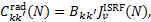
3 Level populations

In molecular clouds, rovibrational levels of H₂ are populated by radiative excitation due to UV photons of the interstellar radiation field (ISRF), by collisions with CR particles (mostly protons, primary and secondary electrons), and by collisions with ambient particles; H₂ levels are depopulated by spontaneous emission and de-excitation by collision with ambient particles.

The equations governing the population and depopulation of a level XvJ the ground electronic level and of a generic excited electronic level SvJ are $\begin{array}{l} n_{X U J} (\sum_{U^{'} J^{'} < u J} A_{X U J \to X_{U^{'} J^{'}}} + \sum_{U^{'} J^{'}} C_{X U J \to X U^{'} J^{'}} + \sum_{S U^{'} J^{'}} C_{X U J \to S U^{'} J^{'}}) = \\ \sum_{v^{'} J^{'} > U^{'} J} n_{X U^{'} J^{'}} A_{X_{U^{'} J^{'}} \to X_{v J} J} + \sum_{U^{'} J^{'}} n_{X U^{'} J^{'}} C_{X U^{'} J^{'} \to X_{v} J} + \sum_{S v^{'} J^{'}} n_{S v^{'} J^{'}} A_{S v^{'} J^{'} \to X_{0} J} \end{array}$ $\eqalign{ & {n_{XUJ}}\left( {\sum\limits_{{U^\prime }{J^\prime } < uJ} {{A_{XUJ \to {X_{{U^\prime }{J^\prime }}}}}} + \sum\limits_{{U^\prime }{J^\prime }} {{C_{XUJ \to X{U^\prime }{J^\prime }}}} + \sum\limits_{S{U^\prime }{J^\prime }} {{C_{XUJ \to S{U^\prime }{J^\prime }}}} } \right) = \cr & \sum\limits_{{v^\prime }{J^\prime } > {U^\prime }J} {{n_{X{U^\prime }{J^\prime }}}} {A_{{X_{{U^\prime }{J^\prime }}} \to {X_{vJ}}J}} + \sum\limits_{{U^\prime }{J^\prime }} {{n_{X{U^\prime }{J^\prime }}}} {C_{X{U^\prime }{J^\prime } \to {X_v}J}} + \sum\limits_{S{v^\prime }{J^\prime }} {{n_{S{v^\prime }{J^\prime }}}} {A_{S{v^\prime }{J^\prime } \to {X_0}J}} \cr}$ (2)

and $n_{S v J} (\sum_{v^{'} J^{'} < u J} A_{S v J \to X v^{'} J^{'}} + \int {\tilde{A}}_{S v J \to X c} d v) = \sum_{v^{'} J^{'}} n_{X v^{'} J^{'}} C_{X v^{'} J^{'} \to S v J},$ ${n_{SvJ}}\left( {\mathop \sum \limits_{v'J' < uJ} {A_{SvJ \to Xv'J'}} + \mathop \smallint \nolimits^ {{\mathop A\limits^ }_{SvJ \to Xc}}{\rm{d}}v} \right) = \mathop \sum \limits_{v'J'} {n_{Xv'J'}}{C_{Xv'J' \to SvJ}},$ (3)

respectively. In the above equations, the transitions' vibrational and rotational quantum numbers are labelled v, v′ , and J, J′ , respectively, while the subscript c represents the continuum of the ground electronic state. Rates of spontaneous emission are denoted by A_kk′, while excitation and de-excitation rates by C_kk′, where kk′ denotes a generic transition from a level k to a level k′ in shorthand notation (i.e. k represents a triplet XvJ or SvJ). The excitation and de-excitation rates, C_kk′, contain a contribution from photons of the ISRF $(C_{k k^{'}}^{rad})$ $\left( {C_{k{k^\prime }}^{{\rm{rad}}}} \right)$ , and a contribution from collisions with CRs and cloud particles. Stimulated emission is neglected. Collisional excitation is dominated by CR electrons $(C_{k k^{'}}^{CR})$ $\left( {C_{k{k^\prime }}^{{\rm{CR}}}} \right)$ and collisional de-excitation by cloud particles $(C_{k k^{'}}^{cl})$ $\left( {C_{k{k^\prime }}^{{\rm{cl}}}} \right)$ , in particular by collisions with ambient H₂. Thus, $C_{k k^{'}} = C_{k k^{'}}^{rad} + C_{k k^{'}}^{CR} + C_{k k^{'}}^{cl}$ ${C_{k{k^\prime }}} = C_{k{k^\prime }}^{{\rm{rad}}} + C_{k{k^\prime }}^{{\rm{CR}}} + C_{k{k^\prime }}^{{\rm{cl}}}$ .

As shown by Eq. (3), H₂ in rovibrational levels within an excited electronic state, S, can either decay back to a bound rovibrational level of the ground electronic state, X, with transition probability A_{SvJ→Xv′J′} or decay into the continuum of the ground state and dissociate, with the transition probability per unit frequency Ã_SvJ→Xc. In the latter case, we assume that the dissociated H₂ converts back to H₂ in the v = 0 level of the ground state and is partitioned into the J = 0 and J = 1 rotational levels depending on the assumed H₂ ortho-to-para (o:p) ratio.

We now turn to examine the excitation processes in detail.

3.1 Radiative excitation

Radiative excitation rates are $C_{k k^{'}}^{rad} (N) = B_{k k^{'}} J_{v}^{ISRF} (N),$ $C_{kk'}^{{\rm{rad}}}(N) = {B_{kk'}}J_v^{{\rm{ISRF}}}(N),$ (4)

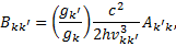where $B_{k k^{'}} = (\frac{g_{k^{'}}}{g_{k}}) \frac{c^{2}}{2 h v_{k k^{'}}^{3}} A_{k^{'} k},$ ${B_{kk'}} = \left( {{{{g_{k'}}} \over {{g_k}}}} \right){{{c^2}} \over {2hv_{kk'}^3}}{A_{k'k}},$ (5)

𝑔_k (𝑔k′) is the degeneracy of state k (k′), and $J_{v}^{ISRF} (N)$ $J_v^{{\rm{ISRF}}}(N)$ is the mean intensity of the ISRF at the transition frequency v_kk′ and at the H₂ column density N. We adopted the radiation field of Draine (1978) and van Dishoeck & Black (1982), whose intensity is characterised by a scaling factor χ (χ = 1 corresponds to the UV ISRF field at 100 nm).

3.2 CR collisional excitation

To obtain CR excitation rates, the cross sections described above must be folded with the spectrum of CR particles (protons, primary and secondary electrons)⁴. For each transition k → k′, CR-induced collisional excitation rates (dropping the subscript kk for simplicity) are 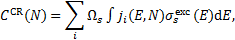$C^{CR} (N) = \sum_{i} Ω_{s} \int j_{i} (E, N) σ_{s}^{exc} (E) d E,$ ${C^{{\rm{CR}}}}(N) = \mathop \sum \limits_i {\Omega _s}\mathop \smallint \nolimits^ {j_i}(E,N)\sigma _s^{{\rm{exc}}}(E){\rm{d}}E,$ (6)

where i is the CR particle species considered (CR protons, primary CR electrons, and secondary electrons), j_s(E, N) is the particle spectrum at column density N (see Sect. 3.1) and $σ_{s}^{exc} (E)$ $\sigma _s^{{\mathop{\rm exc}\nolimits} }(E)$ is the excitation cross section. Taking into consideration a semi-infinite slab configuration, a value of Ω_s = 2π sr is assigned to primary CR nuclei and electrons, while secondary electrons, generated locally and exhibiting nearly isotropic propagation, are attributed a value of Ω_s = 4π sr.

Table 1

Parameters of the Galactic CR electron and proton spectra, Eq. (7).

3.3 Spectrum of secondary electrons

For the calculation of the CR spectrum of secondary electrons at depth N into a semi-infinite cloud, we followed the modelisation developed by Padovani et al. (2009) and Ivlev et al. (2021). In particular, at the cloud’s surface we assumed an interstellar CR spectrum parametrised as in Padovani et al. (2018b), 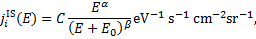$j_{i}^{IS} (E) = C \frac{E^{α}}{{(E + E_{0})}^{β}} {eV}^{- 1} s^{- 1} {cm}^{- 2} {sr}^{- 1},$ $j_i^{{\rm{IS}}}(E) = C{{{E^\alpha }} \over {{{\left( {E + {E_0}} \right)}^\beta }}}{\rm{e}}{{\rm{V}}^{ - 1}}{{\rm{s}}^{ - 1}}{\rm{c}}{{\rm{m}}^{ - 2}}{\rm{s}}{{\rm{r}}^{ - 1}},$ (7)

where i = e, p and E is in eV. Primary CR electrons have a negligible effect on both ionisation and excitation of H₂ above column densities of ≈10²¹ cm⁻² (see Padovani et al. 2022). Therefore, we considered a single spectrum of CR electrons. For primary CR protons, we explored values of the low-energy spectral slope α ranging from α = 0.1 to α = −1.2. In particular, we show results for α = 0.1 (labelled 'low' spectrum, ℒ), which reproduces the proton flux detected by the Voyager probes; α = −0.8 (labelled 'high' spectrum, ℋ), which results in an average value of the ionisation rate estimated in diffuse molecular regions; and α = −1.2 (labelled 'upmost' spectrum, 𝒰), which produces values of the ionisation rate that match the upper envelope of the available observational estimates (see Padovani et al. 2022 and Appendix B for an updated plot of the CR ionisation measurements). Table 1 lists the parameters for the Galactic CR spectrum.

The interstellar spectrum given by Eq. (7) is propagated deep into the cloud under the assumption of continuous slowing-down approximation (see e.g. Takayanagi 1973) adopting the recently updated energy loss functions of protons and electrons colliding with H₂ (see Appendix C). Figure 1 shows the secondary-electron spectra at 10²⁰ and 10²⁴ cm⁻² derived from the three CR proton models (ℒ, ℋ, 𝒰) compared to some representative electron excitation cross sections. The largest contribution to C^CR occurs around E ≈ 20 eV for excitation to the singlet B, C, B′, and D states and E ≈ 14 eV for excitation to the triplet a state. However, to recover 95% of the CR excitation rate for the singlet B, C, B′, and D states, it is necessary to integrate the cross sections from the threshold energy up to ~250 eV (but only up to ~20 eV for the triplet a state, given the sharp decline in energy of the cross section). Thus, the majority of collision-induced excitation to singlet electronic states stems from a broad energy range of secondary electrons. In contrast, considering 30 eV monoenergetic electrons, only about 30% of the total col-lisional excitation rate is recovered, reinforcing the importance of considering the secondary electron spectrum in its entirety.

3.4 De-excitation by collisions with ambient cloud H₂

We included in the coefficients $C_{k k^{'}}^{cl}$ $C_{k{k^\prime }}^{{\rm{cl}}}$ the de-excitation of rotational transitions in the v = 0 level of the ground electronic state of H₂ due to collisions with ambient cloud H₂ (Hernández et al. 2021). We ignored collisions with He and other species.

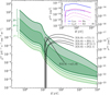Fig. 1

Secondary-electron spectra compared to some electron excitation cross sections for singlet B, C, B′, and D and triplet a states as a function of the energy (Scarlett et al. 2023). The green-scale shaded regions enclose the secondary-electron spectra calculated at N = 10²⁰ cm⁻² (upper boundary) and 10²⁴ cm⁻² (lower boundary) for the three Galactic CR proton models (ℒ, ℋ, 𝒰). The five cross sections shown in black solid lines are the strongest ones for the excitation of the B, C, B′, and D singlet states and the triplet a state from the ground state X(0, 0). The inset shows the electron excitation cross section of atomic hydrogen leading to Lyman and Balmer lines (Möhlmann et al. 1977; Karolis & Harting 1978; van Zyl et al. 1989; Ajello et al. 1991, 1996).

3.5 Comparison between radiative and CR excitation rates

Figure 2 shows our new set of rovibrationally resolved collisional excitation rates normalised to the CR ionisation rate, ζH₂ , obtained by considering the three Galactic CR proton spectra ℒ, ℋ, and 𝒰 introduced in Sect. 3.3. In this figure we only show the results for model ℋ and N = 10²⁰ cm⁻² since the ratio C^CR/ζH₂ is almost independent of the column density, decreasing by only ~20% from 10²⁰ to 10²⁴ cm⁻². Collisional excitation rates increase when using CR proton spectra with a larger component at low energies, since secondary electron fluxes are larger as well (see Fig. 1), and are on average in the following ratios: C^𝒰 : C^ℋ : C^ℒ ≃ 90 : 9 : 1 for the X → B, C, B′, D transitions and 80 : 8 : 1 for the X → a transitions at N = 10²⁰ cm⁻² with a dispersion of ≈2%. These ratios tend to be smaller at larger column densities, since low-energy CRs are stopped locally, and the local CR spectrum becomes independent of the assumption on the low-energy slope. For example, at N = 10²⁴ cm⁻² the above ratios become C^𝒰 : C^ℋ : C^ℒ ≃ 5 : 3 : 1 for X → B, C, B′, D, a transitions with a dispersion of ≲1%.

The top-leftmost panel of Fig. 2 shows the comparison of our C^CR/ζH₂ ratios with those previously computed by Cecchi-Pestellini & Aiello (1992). The latter are limited to the fundamental vibrational level of the ground state, v = 0, and use the cross sections for singlet-state excitation by Shemansky et al. (1985). Since these cross sections are not rotationally resolved, in this figure we sum our collisional excitation rates over all the initial and final rotationally states. Besides, we limit the comparison up to v = 20 for X → B and v = 9 for X → C for a better comparison with Cecchi-Pestellini & Aiello (1992). Our new collisional excitation rates are between 30 and 60% higher than those of Cecchi-Pestellini & Aiello (1992), depending on the CR proton spectrum assumed and the H₂ column density.

We can compare the relative contribution of radiative and collisional excitation rates as a function of column density. Figure 3 shows the histograms of the logarithmic ratio log₁₀(C^CR/C^rad) for all (X), v, J → (B,C, B′, D), v′, J′ common transitions of the two excitation mechanisms as a function of N, for an interstellar UV field with χ = 1, and for model ℋ. We also accounted for different values of R_V, which is a measure of the slope of the extinction at visible wavelengths, computed by Li & Draine (2001), Weingartner & Draine (2001), and Draine (2003a,b,c) for different mixed grain sizes and composition⁵.

In Fig. 3, we consider R_V = 3.1. At column densities lower than 10²¹ cm⁻², radiative excitation dominates since interstellar UV photons are still able to penetrate molecular clouds. At Ν ≈ 10²¹ cm⁻² the two excitation processes contribute on average with equal weight. At larger column densities, the interstellar UV field is completely attenuated, and CRs, in particular secondary electrons, remain the only agents controlling the populations of the excited levels of H₂. As χ varies, the ratio C^CR/C^rad changes by the inverse of the same factor.

Although in this paper we mainly show the results for R_V = 3.1, we also considered the cases R_V = 4.0 and 5.5. As R_V increases, the distribution of log₁₀(C^CR/C^rad) is shifted to smaller values as N, meaning that radiative excitation dominates deeper into the cloud. This is because, as R_V increases, the extinction cross section decreases in the wavelength range 72–180 nm, namely where H₂ bound-bound transitions occur (see Sect. 5).

For the sake of completeness, in Fig. 4, we show histograms of the logarithmic ratio log₁₀(C^CR/C^rad) for models ℒ and 𝒰. As might be expected, since model ℒ has a smaller flux of CR protons at low energies, the histogram has the same pattern as that for the model ℋ , but shifted to smaller log₁₀(C^CR/C^rad) values. This means that higher column densities are required for collisional excitation to dominate radiative excitation. The opposite is true for model 𝒰: due to the higher flux of CR protons at low energies, collisional excitation already dominates radiative excitation at lower column densities.

A comparison with the C^CR computed by Gredel et al. (1989) is presented in Appendix A.

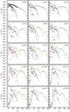Fig. 2

Ratio between the e-H2 excitation rates summed over the initial and final rotational states and the CR ionisation rate for model ℋ and N = 10²⁰ cm⁻² as a function of the upper vibrational level, vu. Each subplot shows results for a different lower vibrational level, v_l. Solid green, violet, magenta, blue, and orange circles refer to the excitation of the B, C, B′, D, and a states from the ground state X, respectively. Empty black circles show a subset of previous estimates by Cecchi-Pestellini & Aiello (1992, see Sect. 3.5 for more details.)

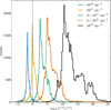Fig. 3

Histograms of the ratio between collisional and radiative excitation rates, C^CR/C^rad, for five representative column densities, from 10²⁰ to 10²² cm⁻², for an interstellar UV field with χ = 1, R_V = 3.1, and model ℋ. The black dashed line shows where collisional and radiative processes equally contribute to excitation of H₂.

Fig. 4

Same as Fig. 3, but for models ℒ (thick lines) and 𝒰 (thin lines).

4 Ultraviolet photon spectrum: Methodology

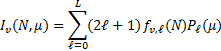
Thanks to the availability of rotationally resolved spontaneous emission coefficients and collisional excitation rates, we were able to determine the level population of each rovibrational level of the X, B, C, Β′, D, Β″, D′ and a states (Eqs. (2) and (3)) and calculate the UV emission of H₂ resolved in its rovi-brational transitions (lines plus continuum), as a function of the assumed interstellar CR spectrum, H₂ column density N, intensity of the interstellar UV field χ H₂ o:p ratio, and dust properties. To compute the radiative transfer of UV radiation in a semi-infinite plane-parallel cloud with embedded sources, we adopted the spherical harmonics method of Roberge (1983). The specific intensity of radiation in the cloud, I_ν(Ν, μ), is expanded in a truncated series of finite odd order L of Legendre polynomials, P_ℓ(μ), as $I_{v} (N, μ) = \sum_{ℓ = 0}^{L} (2 ℓ + 1) f_{v, ℓ} (N) P_{ℓ} (μ)$ ${I_v}(N,\mu ) = \mathop \sum \limits_{\ell = 0}^L (2\ell + 1){f_{v,\ell }}(N){P_\ell }(\mu )$ (8)

where μ is the cosine of the angle of propagation of the radiation. The mean intensity, J_v(N), in units of energy per unit area, time, frequency, and solid angle, is defined as the average of the specific intensity over all solid angles, that is, 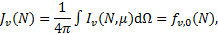$J_{v} (N) = \frac{1}{4 π} \int I_{v} (N, μ) dΩ = f_{v, 0} (N),$ ${J_v}(N) = {1 \over {4\pi }}\mathop \smallint \nolimits^ {I_v}(N,\mu ){\rm{d}}\Omega = {f_{v,0}}(N),$ (9)

where f_v,0(N) is the first coefficient (ℓ = 0) in Eq. (8). The specific flux, F_v(Ν), in units of energy per unit area, time, and frequency, is $F_{v} (N) = \int I_{v} (N, μ) μ dΩ = 4 π f_{v, 1} (N),$ ${F_v}(N) = \mathop \smallint \nolimits^ {I_v}(N,\mu )\mu {\rm{d}}\Omega = 4\pi {f_{v,1}}(N),$ (10)

so that the integrated flux, Φ_UV, in units of photons per unit area and time, is 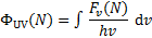$Φ_{UV} (N) = \int \frac{F_{v} (N)}{h v} d v$ ${\Phi _{{\rm{UV}}}}(N) = \mathop \smallint \nolimits^ {{{F_v}(N)} \over {hv}}{\rm{d}}v$ (11)

where h is the Planck constant. Following Roberge (1983), f_v,ℓ (N) at a given column density can be expressed as the sum of two terms, $f_{v, ℓ}^{-} (N)$ $f_{v,\ell }^ - (N)$ and $f_{v, ℓ}^{+} (N)$ $f_{v,\ell }^ + (N)$ , representing the contribution from 0 to N and from N to N_tot, respectively, where N_tot is the total observed line-of-sight H₂ column density. These two terms read as $\begin{array}{l} f_{v, ℓ}^{-} (N) = \sum_{m = 1}^{M} R_{ℓ, m} {C_{- m} e x p [k_{m} (2 σ_{v}^{att} N \\ + \sum_{k k^{'}} \int_{0}^{N} σ_{v, k k^{'}} x_{k} (N^{'}) d N^{'})] + {\hat{Z}}_{v, m} (N)} \end{array}$ $\matrix{ {f_{v,\ell }^ - (N) = \mathop \sum \limits_{m = 1}^M {R_{\ell ,m}}\{ {C_{ - m}}{\rm{ }}e{\rm{ }}x{\rm{ }}p{\rm{ }}[{k_m}(2\sigma _v^{{\rm{att}}}N} \hfill \cr {\,\,\,\,\,\,\,\,\,\,\,\,\,\,\,\,\,\,\, + \mathop \sum \limits_{kk'} \mathop \smallint \limits_0^N {\sigma _{v,kk'}}{x_k}\left( {N'} \right){\rm{d}}N')] + {{\hat Z}_{v,m}}(N)\} } \hfill \cr }$ (12)

and $\begin{array}{l} f_{v, ℓ}^{+} (N) = \sum_{m = 1}^{M} R_{ℓ, m} (C_{m} e x p {- k_{m} [2 σ_{v}^{att} (N_{tot} - N) \\ + \sum_{k k^{'}} \int_{N}^{N_{tot}} σ_{v, k k^{'}} x_{k} (N^{'}) d N^{'}]} + {\hat{W}}_{v, m} (N)) . \end{array}$ $\matrix{ {f_{v,\ell }^ + (N) = \mathop \sum \limits_{m = 1}^M {R_{\ell ,m}}({C_m}{\rm{ }}e{\rm{ }}x{\rm{ }}p{\rm{ }}\{ - {k_m}[2\sigma _v^{{\rm{att}}}\left( {{N_{{\rm{tot}}}} - N} \right)} \hfill \cr {\,\,\,\,\,\,\,\,\,\,\,\,\,\,\,\,\,\,\,\, + \mathop \sum \limits_{kk'} \mathop \smallint \limits_N^{{N_{{\rm{tot}}}}} {\sigma _{v,kk'}}{x_k}\left( {N'} \right){\rm{d}}N']\} + {{\hat W}_{v,m}}(N)).} \hfill \cr }$ (13)

Here, m = ±1,…,±M, where M = (L + 1)/2, k_m and R_ℓ,m are the eigenvalues and the elements of the eigenvector matrix, respectively, of the associated system of linear first-order differential equations (see appendix of Roberge 1983 for details); σ_v,kk′ are the H₂ photoabsorption cross sections from level k, with fractional abundance x_k, to level k′ and the sum over kk′ in Eqs. (12) and (13) extends over all transitions that contribute to absorption at frequency $v; σ_{v}^{att} = σ_{v}^{ext} + \underset{s}{Σ} x_{s} σ_{v, s}^{abs}$ $v;\sigma _v^{{\rm{att}}} = \sigma _v^{{\rm{ext}}} + \sum\limits_s {{x_s}} \sigma _{v,s}^{{\rm{abs}}}$ is the total attenuation cross section per hydrogen nucleus given by the sum of the dust extinction cross section per hydrogen nucleus $(σ_{v}^{ext})$ $\left( {\sigma _v^{{\rm{ext}}}} \right)$ , which is a function of R_v (Draine 2003a), and the photoabsorp-tion cross sections of gas species s with abundance relative to hydrogen nuclei equal to x_s. We only included the most abundant species in the gas phase (H, CO, and N₂) that can cause absorption (shielding) of the photon flux at the H₂ column densities of interest, namely above 3−4 × 10²¹ cm⁻², where the UV ISRF is completely attenuated. For simplicity, following Heays et al. (2017), we assumed constant abundances for these three species⁶: x_H = 10⁻⁴ and $x_{CO} = x_{N_{2}} = 10^{- 5}$ ${x_{{\rm{CO}}}} = {x_{{{\rm{N}}_2}}} = {10^{ - 5}}$ . The photoabsorption cross sections $σ_{v, s}^{abs}$ $\sigma _{v,s}^{{\rm{abs}}}$ are taken from the Leiden Observatory database (see also Heays et al. 2017). For each transition k → k′, the H₂ photoabsorption cross section is $σ_{v, k k^{'}} = \frac{1}{4 π} B_{k k^{'}} h v_{k k^{'}} ϕ_{v}$ ${\sigma _{v,kk'}} = {1 \over {4\pi }}{B_{kk'}}h{v_{kk'}}{\phi _v}$ (14)

where ϕ_ν is the line profile, and ν is the frequency of the transition. We note that we were able to treat H₂ self-absorption line by line since with the procedure described in Sect. 2 we could calculate the population of each rovibrational level. Figure 5 shows the contribution of dust and gas (H₂, H, CO, and N₂) absorption to the optical depth at the H₂ column density N = 10²¹ cm⁻². We note that the overlapping line wings of the H₂ transitions plus the CO, N₂, and H lines produce a net opacity that exceeds the dust opacity over a large fraction of the wavelength range 72–130 nm. Therefore, it is important to include in Eqs. (12) and (13) an explicit sum over all transitions contributing to the emission at frequency ν in order to account for overlaps and blending.

The functions ${\hat{Z}}_{v, m} (N) and {\hat{W}}_{v, m} (N)$ ${\hat Z_{v,m}}(N){\rm{ and }}{\hat W_{v,m}}(N)$ describe the contribution of isotropic embedded sources and are ${\hat{Z}}_{v, m} (N) = \frac{k_{m}}{1 - ω_{v}} R_{m, 0}^{- 1} ℐ_{v, m}^{Z} (N)$ ${\hat Z_{v,m}}(N) = {{{k_m}} \over {1 - {\omega _v}}}R_{m,0}^{ - 1}{\cal I}_{v,m}^Z(N)$ (15)

and ${\hat{W}}_{v, m} (N) = \frac{k_{m}}{1 - ω_{v}} R_{m, 0}^{- 1} I_{v, m}^{W} (N),$ ${\hat W_{v,m}}(N) = {{{k_m}} \over {1 - {\omega _v}}}R_{m,0}^{ - 1}I_{v,m}^W(N),$ (16)

where ω_ν is the dust albedo, while $\begin{array}{l} I_{v, m}^{Z} (N) = \int_{0}^{N} S_{v} (N^{'}) \exp [- 2 σ_{v}^{att} k_{m} (N - N^{'})] \\ \times \exp [- k_{m} \sum_{k k^{'}} \int_{N^{'}}^{N} σ_{v, k k^{'}} x_{k} (N^{''}) d N^{''}] d N^{'} \end{array}$ $\matrix{ {I_{v,m}^{\rm{Z}}(N) = \mathop \smallint \limits_0^N {S_v}\left( {N'} \right)\exp \left[ { - 2\sigma _v^{{\rm{att}}}{k_m}\left( {N - N'} \right)} \right]} \hfill \cr {\,\,\,\,\,\,\,\,\,\,\,\,\,\,\,\,\,\,\,\,\,\,\, \times \exp \left[ { - {k_m}\mathop \sum \limits_{kk'} \mathop \smallint \limits_{N'}^N {\sigma _{v,kk'}}{x_k}\left( {N''} \right){\rm{d}}N''} \right]{\rm{d}}N'} \hfill \cr }$ (17)

and $\begin{array}{l} I_{v, m}^{W} (N) = \int_{N}^{N_{tot}} S_{v} (N^{'}) \exp [- 2 σ_{v}^{att} k_{m} (N^{'} - N)] \\ \times \exp [- k_{m} \sum_{k k^{'}} \int_{N}^{N^{'}} σ_{v, k k^{'}} x_{k} (N^{''}) d N^{''}] d N^{'} \end{array}$ $\matrix{ {I_{v,m}^W(N) = \mathop \smallint \limits_N^{{N_{{\rm{tot}}}}} {S_v}\left( {N'} \right)\exp \left[ { - 2\sigma _v^{{\rm{att}}}{k_m}\left( {N' - N} \right)} \right]} \hfill \cr {\,\,\,\,\,\,\,\,\,\,\,\,\,\,\,\,\,\,\, \times \exp \left[ { - {k_m}\mathop \sum \limits_{kk'} \mathop \smallint \limits_N^{N'} {\sigma _{v,kk'}}{x_k}\left( {N''} \right){\rm{d}}N''} \right]{\rm{d}}N'} \hfill \cr }$ (18)

Here, the source function is $S_{v} (N) = \frac{1}{4 π} [\sum_{k k^{'}} x_{k^{'}} (N) A_{k^{'} k} h v_{k k^{'}} ϕ_{v} + \sum_{k^{'}} x_{k^{'}} (N) {\tilde{A}}_{k^{'} c} E_{t}],$ ${S_v}(N) = {1 \over {4\pi }}\left[ {\mathop \sum \limits_{kk'} {x_{k'}}(N){A_{k'k}}h{v_{kk'}}{\phi _v} + \mathop \sum \limits_{k'} {x_{k'}}(N){{\mathop A\limits^ }_{k'c}}{E_t}} \right],$ (19)

where A_k′k is the transition probability from level k′ to k, and Ã_k′c is the transition probability per unit frequency from level k′ to the continuum of the ground electronic state (c), with transition energy E_t.

Finally, the constants C_m in Eqs. (12) and (13) are obtained from Mark’s conditions (Mark 1944, 1945) by inverting the system of equations $\sum_{m = - M}^{M} ℬ_{i m} C_{m} = Q_{i}$ $\mathop \sum \limits_{m = - M}^M {{\cal B}_{im}}{C_m} = {Q_i}$ (20)

with i = 1,…, 2M, where $2 ℬ_{i m} = {\begin{array}{l} \sum_{ℓ = 0}^{L} (2 ℓ + 1) P_{ℓ} (μ_{i}) R_{l m}, & (μ_{i} < 0 \land m < 0) \lor (μ_{i} > 0 \land m > 0) \\ \sum_{ℓ = 0}^{L} (2 ℓ + 1) P_{ℓ} (μ_{i}) R_{l m} e^{ε_{v, m}}, & (μ_{i} < 0 \land m > 0) \lor (μ_{i} > 0 \land m < 0), \end{array}$ $2{{\cal B}_{im}} = \{ \matrix{ {\mathop \sum \limits_{\ell = 0}^L (2\ell + 1){P_\ell }\left( {{\mu _i}} \right){R_{lm}},} \hfill & {\left( {{\mu _i} < 0 \wedge m < 0} \right) \vee \left( {{\mu _i} > 0 \wedge m > 0} \right)} \hfill \cr {\mathop \sum \limits_{\ell = 0}^L (2\ell + 1){P_\ell }\left( {{\mu _i}} \right){R_{lm}}{e^{{\varepsilon _{v,m}}}},} \hfill & {\left( {{\mu _i}\left\langle {0 \wedge m} \right\rangle 0} \right) \vee \left( {{\mu _i} > 0 \wedge m < 0} \right),} \hfill \cr }$ (21)

with $ℰ_{v, m} = - | 2 k_{m} [- (2 σ_{v}^{att} \frac{N_{tot}}{2} + \sum_{k k^{'}} \int_{0}^{N_{tot} / 2} σ_{v, k k^{'}} x_{k} (N^{'}) d N^{'})] |$ ${{\cal E}_{v,m}} = - \left| {2{k_m}\left[ { - \left( {2\sigma _v^{{\rm{att}}}{{{N_{{\rm{tot}}}}} \over 2} + \mathop \sum \limits_{kk'} \mathop \smallint \limits_0^{{N_{{\rm{tot}}}}/2} {\sigma _{v,kk'}}{x_k}\left( {N'} \right){\rm{d}}N'} \right)} \right]} \right|$ (22)

and $Q_{i} = {\begin{array}{l} I_{v}^{-} (μ_{i}) - \sum_{ℓ = 0}^{L} (2 ℓ + 1) P_{ℓ} (μ_{i}) \sum_{m = 1}^{M} R_{ℓ, - m} {\hat{Z}}_{v, m} (N_{tot}), & μ_{i} > 0 \\ I_{v}^{+} (μ_{i}) - \sum_{ℓ = 0}^{L} (2 ℓ + 1) P_{ℓ} (μ_{i}) \sum_{m = 1}^{M} R_{ℓ m} {\hat{W}}_{v, m} (0), & μ_{i} < 0. \end{array}$ ${Q_i} = \{ \matrix{ {I_v^ - \left( {{\mu _i}} \right) - \mathop \sum \limits_{\ell = 0}^L (2\ell + 1){P_\ell }\left( {{\mu _i}} \right)\mathop \sum \limits_{m = 1}^M {R_{\ell , - m}}{{\hat Z}_{v,m}}\left( {{N_{{\rm{tot}}}}} \right),} \hfill & {{\mu _i} > 0} \hfill \cr {I_v^ + \left( {{\mu _i}} \right) - \mathop \sum \limits_{\ell = 0}^L (2\ell + 1){P_\ell }\left( {{\mu _i}} \right)\mathop \sum \limits_{m = 1}^M {R_{\ell m}}{{\hat W}_{v,m}}(0),} \hfill & {{\mu _i} < 0.} \hfill \cr }$ (23)

The sums in Eqs. (19) and (22) are performed over all transitions contributing to the emission at frequency . In Eq. (22), $I_{v}^{-} and I_{v}^{+}$ $I_v^ - {\rm{and }}I_v^ +$ represent the external field impinging on the two sides of the cloud. In most cases, one considers a semi-infinite cloud. This happens, for example, in astrochemical databases where photodissociation and photoionisation rates are given as a function of the visual extinction or the column density. In this case $J_{v} (N) = f_{v, 0}^{-} (N)$ ${J_v}(N) = f_{v,0}^ - (N)$ , while for clouds irradiated from two sides, $J_{v} (N) = f_{v, 0}^{-} (N) + f_{v, 0}^{+} (N)$ ${J_v}(N) = f_{v,0}^ - (N) + f_{v,0}^ + (N)$ .

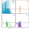Fig. 5

Comparison of the optical depth, τ, of dust (black solid lines) to that of para- and ortho-H₂ (blue and cyan solid lines, respectively, upper-left panel), H (orange solid lines, upper-right panel), CO (green solid lines, bottom-left panel), and N₂ (purple solid lines, bottom-right panel) at N(H₂) = 10²¹ cm⁻². The H₂ optical depth is shown for model ℋ and H₂ o:p = 3:1. The H, CO, and N₂ optical depths have been computed by assuming constant abundances $(x_{H} = 10^{- 4}, x_{CO} = x_{N_{2}} = 10^{- 5})$ $\left( {{x_{\rm{H}}} = {{10}^{ - 4}},{x_{{\rm{CO}}}} = {x_{{{\rm{N}}_2}}} = } \right.{10^{ - 5}})$ and the photoabsorption cross sections presented in the Leiden Observatory database (https://home.strw.leidenuniv.nl/~ewine/photo/; see also Heays et al. 2017).

5 Ultraviolet photon spectrum: Results

In this section, we show the results for typical conditions in the densest regions of molecular clouds, characterised by a temperature of 10 K and a turbulent line broadening of 1 km s⁻¹. These two parameters determine the Gaussian profile, to be combined with the natural Lorentzian linewidth. We assumed that ortho-para conversions due to reactive collisions with protons are not frequent in molecular clouds (Flower & Watt 1984) and we examined the two extreme cases where the H₂ o:p ratio is equal to 0:1 (H₂ in para form) and to 1:0 (H₂ in ortho form). Under this hypothesis, since the ortho and para states in this framework are not coupled by any process, the results for the para-H₂ and ortho-H₂ cases (presented in Sect. 6 and Appendix D) can be linearly combined for any arbitrary o:p ratios.

Figures 6 and 7 show the para-H₂ and ortho-H₂ line spectra, respectively. Each panel illustrates the partial spectrum due to the transitions from an excited electronic state (B, C, B′, D, B″, D′) to the ground state X. As an illustration, results are shown for N = 10²³ cm⁻² assuming the CR proton flux of model ℋ and R_V = 3.1.

Although spontaneous emission rates for B″ → X and D′ → X transitions are currently available only for a limited number of rotational levels (see Sect. 2), their contribution, together with that of the D⁻ → X transitions, is very relevant as they generate significant emission at wavelengths shorter than ~85 nm, roughly corresponding to the lower boundary of the Lyman-Werner bands, where the peak of most photoionisation cross sections is located (Heays et al. 2017; Hrodmarsson & van Dishoeck 2023).

We note that, because of the lack of spontaneous emission rates from J > 1 levels of the D′⁻ state, in the case of pure para-H₂ (Fig. 6), we did not consider the D′⁻ state, as it could not be de-excited if populated. Therefore, there is no associated emission. In a future article, we will consider the emission from all upper rotational levels of the B″ and D′ states.

In the case of pure ortho-H₂ (Fig. 7), the emission from D′⁻ is also present together with the emission resulting from the Q branch of C and D states, namely C⁻ and D⁻. Moreover, the emission from the C⁻ and D⁻ states is much more intense than in the case of pure para-H₂. This is because electronic states with Λ = 1, where Λ is the projection of the electron orbital angular momentum onto the internuclear axis, do not have J = 0 levels. Thus, if all the H₂ is initially in the J = 0 level (pure para-H₂), a large fraction of the emission is missing.

Figures 8 and 9 show the continuum spectra due to each excited electronic state for H₂ o:p=0:1 and H₂ o:p=1:0, respectively. The continuum emission is only longward of about 120 nm. Continuum emission from B″ and D′ states is not included because spontaneous emission rates are not available. We note, however, that the contributions to the continuum emission of Rydberg states with n ≥ 3 are more and more negligible compared to those from n = 2 states. Below 180 nm the continuum is dominated by the emission of the B and C⁺ states in the case o:p=0:1, while in the case o:p=1:0 the C⁻ state also contributes in a small wavelength window, below 130 nm.

Above 180 nm, the continuum emission is entirely due to the triplet a state. Including this emission is crucial as several photodissociation cross sections have their maximum contribution at λ > 180 nm. To give a few examples: NH₃ shows a large number of resonances up to about 220 nm; C₃H₃, AlH, and CS₂ peak around 200 nm; LiH around 270 nm; the S₂ threshold is at about 240 nm; CH₃NH₂ has a tail up to 250 nm; and C₂H₅ has an important contribution above 200 nm (Heays et al. 2017; Hrodmarsson & van Dishoeck 2023).

Finally, in Fig. 10 we show the total specific intensity J_v, including H₂ line and continuum components, H line emission in the Lyman and Balmer series, and the ISRF continuum. We show spectra at four different column densities. The comparison illustrates that the ISRF continuum becomes negligible compared to the line emission around 4 × 10²¹ cm⁻². However, the ISRF still dominates at wavelengths above about 250 nm up to H₂ column densities of the order of 10²² cm⁻², when the H₂ continuum becomes prominent. Atomic hydrogen lines of the Balmer series contribute significantly to the total photon flux (see Sect. 7).

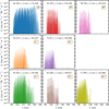Fig. 6

Mean intensity, J_V, of bound-bound H₂ transitions as a function of the wavelength, λ, for a molecular cloud with column density N = 10²³ cm⁻² illuminated by one side. Line spectra are shown separately for each excited electronic state. Results are shown for model ℋ , H₂ o:p=0:1, and R_V = 3.1.

Fig. 7

Same as Fig. 6, but for H₂ o:p = 1:0.

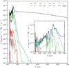Fig. 8

Mean intensity, J_v, of the continuum emission of H₂ from excited electronic states as a function of wavelength, λ, for a molecular cloud with a column density N = 10²³ cm⁻² illuminated by one side. The contribution of each excited electronic state (solid lines) is shown by solid coloured lines, while the dashed black line shows the total continuum emission. The inset shows the emission in the range 120–180 nm. Results are shown for model ℋ, H₂ o:p=0:1, and R_V = 3.1.

Fig. 9

Same as Fig. 8, but for H₂ o:p=1:0.

6 Photorates

In this section we present the calculation of photodissocia-tion and photoionisation rates. This topic has already been extensively examined in previous articles thanks to the crucial advances in the derivation of the photodissociation and photoionisation cross sections of a large number of atomic and molecular species, as presented in the Leiden Observatory database^??, and described by Heays et al. (2017) and by a recent update by Hrodmarsson & van Dishoeck (2023). Previous calculations adopted the H₂ emission spectrum calculated by Gredel et al. (1987, 1989). As a result of recent studies on primary CR propagation (e.g. Padovani et al. 2009, 2018b, 2022), secondary electron generation (Ivlev et al. 2021), rovibrationally resolved collisional excitation cross sections (Scarlett et al. 2023), and spontaneous emission rates (Abgrall et al. 1993a,b,c, 1997, 2000; Liu et al. 2010; Roueff et al. 2019), we have been able to calculate the UV photon spectrum in its line and continuum components (Sects. 4 and 5), and consequently the photorates, with higher accuracy.

The rate of photodissociation or photoionisation, due to CR-generated UV photons, of an atomic or molecular species s as a function of H₂ column density is 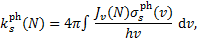$k_{s}^{ph} (N) = 4 π \int \frac{J_{v} (N) σ_{s}^{ph} (v)}{h v} d v,$ $k_s^{{\rm{ph}}}(N) = 4\pi \mathop \smallint \nolimits^ {{{J_v}(N)\sigma _s^{{\rm{ph}}}(v)} \over {hv}}{\rm{d}}v,$ (24)

where J_v(N) is the mean intensity (Eq. (9)) and $σ_{s}^{ph} (v)$ $\sigma _s^{{\rm{ph}}}(v)$ is the photodissociation or photoionisation cross section of the species. We note that J_v(N) takes into account both Doppler broadening and the natural Lorentzian linewidth, so that a Voigt profile is associated with each line. The number of steps for the frequency integration is chosen to have a resolution of at least one-hundredth of the maximum resolution of the cross sections for a given frequency. This adaptive grid has been adopted to account for all details of cross sections.

The dependence on column density lies solely in the assumption of the incident CR spectrum through the CR ionisation rate, $ζ_{H_{2}} (N)$ ${\zeta _{{{\rm{H}}_2}}}(N)$ , parameterised as in Eq. (B.1). Therefore, Eq. (24) can be rewritten as $k_{s}^{ph} (N) = k_{0, s}^{ph} ζ_{H_{2}} (N) .$ $k_s^{{\rm{ph}}}(N) = k_{0,s}^{{\rm{ph}}}{\zeta _{{{\rm{H}}_2}}}(N).$ (25)

Equation (25) does not include the contribution to the pho-todissociation or photoionisation rate of UV photons from the ISRF, which must be added separately. The ISRF contribution is usually parameterised as a function of the visual extinction, whose scaling with H₂ column density is given by the standard proportionality (e.g. Bohlin et al. 1978). Values of $k_{0, s}^{ph}$ $k_{0,s}^{{\rm{ph}}}$ have been computed for a number of species for R_v = 3.1 (Tables D.1 and D.2), R_v = 4.0 (Tables D.3 and D.4), and R_V = 5.5 (Tables D.5 and D.6). While photorates show no appreciable changes from R_V = 3.1 to R_V = 4.0, for R_V = 5.5 they increase on average by 29% ± 14% and 41% ± 9% for photodissociation and photoionisation, respectively, with respect to R_V = 3.1. We use the superscripts 'pd' and 'pi' to refer to the photodissociation and photoionisation constant ( $k_{0, s}^{pd} and k_{0, s}^{pi}$ $k_{0,s}^{{\rm{pd}}}{\rm{and}}k_{0,s}^{{\rm{pi}}}$ , respectively) in Eq. (25). For each of these tables, we tabulate the rates for pure para and pure ortho H₂ form(o:p=0:1 and o:p=1:0, respectively). As anticipated in Sect. 5, since we assume no ortho-para conversion (Flower & Watt 1984), photorates for para and ortho H₂ can be linearly combined, if the o:p ratio as a function of H₂ column density is known. However, the values of $k_{0}^{ph}$ $k_0^{{\rm{ph}}}$ , are comparable on average to within 5% for the two H₂ o:p ratios considered, with only a few species showing slightly larger differences. In particular, $k_{0, s}^{pd}$ $k_{0,s}^{{\rm{pd}}}$ for o:p=0:1 is larger than that for o:p=1:0 by 85% for CO, by 30% for $H_{3}^{+}$ ${\rm{H}}_3^ +$ , and by 25% for C₂H₂ and CS and is lower than that for o:p=1:0 by 25% for HCO+ and N₂; $k_{0}^{pi}$ $k_0^{{\rm{pi}}}$ for o:p=0:1 is larger than that for o:p=1:0 by 40% for CO and Zn, by 35% for N₂, by 30% for CN, and by 25% for O₂.

We compared the new photorate constants, $k_{0, s}^{ph}$ $k_{0,s}^{{\rm{ph}}}$ , with the most recent determination by Heays et al. (2017) and Hrodmarsson & van Dishoeck (2023), who computed the rates assuming $ζ_{H_{2}} = 10^{- 16} s^{- 1}$ ${\zeta _{{{\rm{H}}_2}}} = {10^{ - 16}}{{\rm{s}}^{ - 1}}$ , R_V = 3.1, o:p=0:1, a Doppler broadening of 1 km s⁻¹ , and constant abundances for H, CO, and N₂ $(x_{H} = 10^{- 4}, x_{CO} = x_{N_{2}} = 10^{- 5})$ $\left( {{x_{\rm{H}}} = {{10}^{ - 4}},{x_{{\rm{CO}}}} = {x_{{{\rm{N}}_2}}} = {{10}^{ - 5}}} \right)$ . Our photodissociation and photoionisation rates are, on average, smaller than the previous ones by a factor of 2.2 ± 0.8 and 1.6 ± 0.5, respectively. For species such as $AlH, C_{2} H_{2}, C_{2} H_{3}, C_{3} H_{3}, LiH, N_{2}, NaCl, NaH, O_{2}^{+}, S_{2}, SiH, l - C_{4}$ ${\rm{AlH}},{{\rm{C}}_2}{{\rm{H}}_2},{{\rm{C}}_2}{{\rm{H}}_3},{{\rm{C}}_3}{{\rm{H}}_3},{\rm{LiH}},{{\rm{N}}_2},{\rm{NaCl}},{\rm{NaH}},{\rm{O}}_2^ + ,{{\rm{S}}_2},{\rm{SiH}},{\rm{l}} - {{\rm{C}}_4}$ , and 1-C₅H, our photodissociation rates are lower by a factor of 3 up to 5. The photoionisation rates of H₂, HF, and N₂ deserve special attention. For these species, the ionisation threshold energies are 15.43 eV (Shiner et al. 1993), 16.06 eV (Bieri et al. 1980), and 15.58 eV (Trickl et al. 1989), corresponding to wavelengths of about 80.36 nm, 77.19 nm, and 79.56 nm, respectively. This means that the contribution of photons at shorter wavelengths is crucial for the correct evaluation of the photoionisation rate. Our new calculations extend the photon spectrum down to 72 nm. Within this wavelength range lies a considerable number of transitions from the electronic levels D⁻, B″, D′⁻, and D′⁺ to the ground state X, resulting in an increase in the photoionisation constants, $k_{0, s}^{pi}$ $k_{0,s}^{{\rm{pi}}}$ of approximately 9.4 × 10³, 2 × 10⁵, and 1.2 × 10⁴ for H₂, HF, and N₂, respectively. For the H₂ photodissociation rate, we also find a value larger by a factor of 16 than what was previously found. Again, this is because the H₂ photodissociation cross section extends down to wavelengths of 70 nm and partly because of our line-by-line treatment of H₂ self-absorption.

Fig. 10

Mean intensity, J_v, of the total emission in the wavelength range 72 < λ/nm < 250 for a molecular cloud illuminated by one side. From top to bottom the four panels show the expected mean intensity from H₂ lines, H₂ continuum, H lines (Lyα and Lyβ), and ISRF at four different column densities, from N = 10²¹ to 4 × 10²² cm⁻². Insets show the components of J_v at 400 < λ/nm < 700, highlighting three lines of the Balmer series (Hα, Hβ, and Hγ). Results are shown for model ℋ, χ = 1, H₂o:p=0:1, and R_v = 3.1.

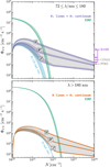Fig. 11

Photon fluxes, Φ_UV, as a function of the H₂ column density, N, below and above 180 nm (upper and lower panel, respectively) for χ = 1. Both panels show the integrated flux of CR-generated UV photons as a function of the three models of CR proton flux (ℒ, ℋ and 𝒰) and the ISRF UV flux. The cyan dotted lines show the integrated photon flux from H₂ and Η lines generated by collisional radiative excitation (labelled 'rad. exc.'). The three curves for each model correspond to R_V = 3.1 (lower curve), 4.0 (intermediate curve), and (5.5 upper curve). Arrows on the righthand side of the upper panel show previous estimates of Φ_UV, independent of column density: Prasad & Tarafdar (1983, PT83), Cecchi-Pestellini & Aiello (1992, CPA92), and Shen et al. (2004, S+04).

7 Integrated ultraviolet photon flux

The CR-generated UV photon flux has drastic consequences on the process of charging of dust grains (see e.g. Ivlev et al. 2015; Ibáñez-Mejía et al. 2019). Through the photoelectric effect, photons can extract electrons from dust grains, thus redistributing the charge. More specifically, this process generates a population of positively charged grains that can then combine with those of opposite charge to form larger and larger conglomerates. This mechanism is particularly relevant as it is linked to the formation of planetesimals and thus planets.

The fundamental parameter governing the equilibrium charge distribution is the integrated photon flux, Φ_UV (Eq. (11)). In Fig. 11, we show the calculation of Φ_UV in two wavelength ranges, below and above 180 nm. This value is chosen to isolate the contribution of the H₂ lines (72 ≲ λ/nm ≲ 180; see Figs. 6 and 7). As can be seen, Φ_UV depends on the selected CR model, while it has a weak dependence on the chosen R_V value. In addition, Φ_UV is independent of the H₂ o:p ratio since it is an integrated quantity, whereas the effect of the H₂ o:p ratio is only to redistribute photons at different wavelengths. The bump seen between Ν = 10²⁰ and 10²² cm⁻² is due to radiative excitation alone, while at higher column density CR-generated UV photons fully determine Φ_UV· Photons at wavelengths larger than 180 nm contribute as much as 20% to the total integrated photon flux above 10²² cm⁻². Besides, the Lyman and Balmer series lines contribute only 3% at λ < 180 nm and up to 40% at λ > 180 nm, respectively, to Φ_UV·

As for the photorates, it turns out that Φ_UV normalised to ζH₂ is also independent of the assumed interstellar CR model. This allows us to parameterise the integrated photon flux solely as a function of column density and R_V as $Φ_{UV} (N) = 10^{3} (c_{0} + c_{1} R_{V} + c_{2} R_{V}^{2}) [\frac{ζ_{H_{2}} (N)}{10^{- 16} s^{- 1}}] {cm}^{- 2} s^{- 1},$ ${\Phi _{{\rm{UV}}}}(N) = {10^3}\left( {{c_0} + {c_1}{R_V} + {c_2}R_V^2} \right)\left[ {{{{\zeta _{{{\rm{H}}_2}}}(N)} \over {{{10}^{ - 16}}{{\rm{s}}^{ - 1}}}}} \right]{\rm{c}}{{\rm{m}}^{ - 2}}{{\rm{s}}^{ - 1}},$ (26)

where c₀ = 5.023, c₁ = −0.504, and c₂ = 0.115. The above fit is valid for 3.1 ≤ R_V ≤ 5.5. Parameterisations of ζH₂(Ν) are given by Eq. (B.l). In principle, Eq. (26) is valid above about Ν = 10²² cm⁻²; however, it can be extrapolated at lower H₂ column densities as well, as the photon flux generated by CRs is negligible with respect to the UV ISRF photons.

The upper panel of Fig. 11 also shows the predictions by Prasad & Tarafdar (1983) and Cecchi-Pestellini & Aiello (1992) who obtained Φ_UV = 1350 cm² s⁻¹ and ≈ 3000 cm² s⁻¹, respectively, assuming ζH₂ = 1.7 × 10⁻¹⁷ s⁻¹, and by Shen et al. (2004) who predict constant Φ_UV values between 1800 and 29 000 cm² s⁻¹, depending on the assumption of three different low-energy CR fluxes, but without accounting for energy losses while CRs propagate.

8 Conclusions

Cosmic rays exert significant influence by regulating the abundance of ions and radicals, leading to the formation of increasingly complex molecular species and influencing the charge distribution on dust grains. Our study emphasises the critical importance of investigating the UV photon flux generated by CR secondary electrons in dense molecular clouds. Building on the seminal works of Roberge (1983), Prasad & Tarafdar (1983), Sternberg et al. (1987), and Gredel et al. (1987, 1989), we examined this topic in the light of significant advances in the field of microphysical processes. Our research benefited from the following advances: (i) accurate calculations of collisional excitation cross sections (Scarlett et al. 2023) and spontaneous emission rates (Abgrall et al. 1993a,b,c, 1997, 2000; Liu et al. 2010; Roueff et al. 2019, Glass-Maujean, priv. comm.), all of which are rotationally resolved; (ii) comprehensive insights into the propagation and attenuation of the Galactic CR flux within molecular clouds (Padovani et al. 2009, 2018b, 2022); and (iii) the robust calculation of secondary electron fluxes resulting from the ionisation of H₂ by CRs (Ivlev et al. 2021).

We were then able to calculate the population of the X ground state, the excited electronic singlet (B, C, B′, D, B″, and D′) and triplet (a) states of molecular hydrogen, and thus the UV spectrum resulting from H₂ de-excitation. We note that this spectrum also includes Lyman and Balmer series lines of atomic hydrogen. From the 1508 rovibrational levels, we produced a UV spectrum consisting of 38 970 lines, spanning from 72 to 700 nm, and studied its variation as a function of the CR spectrum incident on a molecular cloud, the column density of H₂, the isomeric H₂ composition, and the properties of the dust.

Using the most recent and complete databases of photodissociation and photoionisation cross sections of a large number of atomic and molecular species (Heays et al. 2017; Hrodmarsson & van Dishoeck 2023), we calculated the photodissociation and photoionisation rates, giving parameterisations as a function of the H₂ column density through the CR ionisation rate models from Padovani et al. (2022). On average, this new set of rates differs from previous estimates, with reductions of approximately 2.2 ± 0.8 and 1.6 ± 0.5 for photodissociation and photoionisation, respectively. In particular, deviations of up to a factor of 5 are observed for some species, such as AlH, C₂H₂, C₂H₃, C₃H₃, LiH, N₂, NaCl, NaH, $O_{2}^{+}$ ${\rm{O}}_2^ +$ , S₂, SiH, l-C₄, and l-C₅H. Particular consideration should be paid to the significantly higher photoionisation rates of H₂, HF, and N₂, as well as the photodissociation of H₂, which our study revealed to be orders of magnitude higher than previous evaluations. This discrepancy can be attributed to our new calculations extending the photon spectrum down to 72 nm, where the cross sections of these species have a large contribution, and partly to the H₂ self-absorption that we were able to treat line by line.

In addition, we calculated the integrated UV photon flux, regulating the equilibrium charge distribution on dust grains and thus the formation of larger and larger conglomerates. Compared to previous estimates of this quantity that predicted a constant value, we provide a parameterisation as a function of H₂ column density, through the CR ionisation rate, and the dust properties.

Acknowledgements

The authors wish to thank the referee, John Black, for his careful reading of the manuscript and insightful comments that considerably helped to improve the paper. The authors are also grateful to Hervé Abgrall, Martin Čižek, Michèle Glass-Maujean, Isik Kanik, Xianming Liu, Evelyne Roueff, and Jonathan Tennyson for fruitful discussions and feedback. I, M.P., want to leave a memory of my father Piero, a watchmaker.

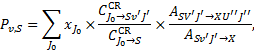
Appendix A Comparison with Gredel et al. (1989)

Gredel et al. (1989), hereafter G89, assume that H₂ is in some v = 0, J = J₀ level(s) of the ground state X, and is collisionally excited by a 30 eV secondary CR electron to a level v′ J′ of an excited electronic state S, from which it spontaneously decay to a level v″J″ of the ground state with probability A_{Sv′J′→Xv″J″}. The probability of emission of a line photon with energy hv = E(Sv′J′) − E(Xv″J″) is $P_{v, S} = \sum_{J_{0}} x_{J_{0}} \times \frac{C_{J_{0} \to S v^{'} J^{'}}^{CR}}{C_{J_{0} \to S}^{CR}} \times \frac{A_{S V^{'} J^{'} \to X U^{''} J^{''}}}{A_{S v^{'} J^{'} \to X}},$ ${P_{v,S}} = \mathop \sum \limits_{{J_0}} {x_{{J_0}}} \times {{C_{{J_0} \to Sv'J'}^{{\rm{CR}}}} \over {C_{{J_0} \to S}^{{\rm{CR}}}}} \times {{{A_{SV'J' \to XU''J''}}} \over {{A_{Sv'J' \to X}}}},$ (A.1)

where $x_{j_{0}}$ ${x_{{j_0}}}$ is the fractional population of each level v = 0, J = J₀ of the ground state, $C_{J_{0} \to S}^{CR}$ $C_{{J_0} \to S}^{{\rm{CR}}}$ is the total collisional excitation rate to all levels v′J′ of state S⁷, $C_{J_{0} \to S}^{CR} = \sum_{v^{'} J^{'}} C_{J_{0} \to S_{J^{'}} J^{'}}^{CR},$ $C_{{J_0} \to S}^{{\rm{CR}}} = \mathop \sum \limits_{v'J'} C_{{J_0} \to {S_{J'}}J'}^{{\rm{CR}}},$ (A.2)

and A_Sv′J′is the total decay rate of the level v′J′ of state S, $A_{S v^{'} J^{'} \to X} = \sum_{U^{''} J^{''}} A_{S v^{'} J^{'} \to X v^{'} J^{''}}$ ${A_{Sv'J' \to X}} = \mathop \sum \limits_{U''J''} {A_{Sv'J' \to Xv'J''}}$ (A.3)

The emission rate R_v of photons of frequency v is then the sum over all S states of the emission probabilities P_v,S multiplied by the total excitation rate $C_{s}^{CR}$ $C_s^{{\rm{CR}}}$ of each state: $R_{v} = \sum_{S} P_{v, S} C_{S}^{CR}$ ${R_v} = \mathop \sum \limits_S {P_{v,S}}C_S^{{\rm{CR}}}$ (A.4)

where $C_{S}^{CR} = \sum_{J_{0}} x_{J_{0}} C_{J_{0} \to S}^{CR}$ $C_S^{{\rm{CR}}} = \mathop \sum \limits_{{J_0}} {x_{{J_0}}}C_{{J_0} \to S}^{{\rm{CR}}}$ (A.5)

For a statistical equilibrium mixture of H₂ with $x_{J_{0} = 0} = 0.25$ ${x_{{J_0} = 0}} = 0.25$ and $x_{J_{0} = 1} = 0.75$ ${x_{{J_0} = 1}} = 0.75$ , G89 obtain the weights listed in Table A. The weights are normalised to $ζ_{H_{2}}$ ${\zeta _{{{\rm{H}}_2}}}$ , the total H₂ ionisation rate (primary plus mono-energetic secondary electrons with energy 30 eV). Our results are shown for comparison⁸.

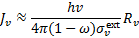
The mean intensity of H₂ line emission in the optically thick limit is then $J_{v} \approx \frac{h v}{4 π (1 - ω) σ_{v}^{ext}} R_{v}$ ${J_v} \approx {{hv} \over {4\pi (1 - \omega )\sigma _v^{{\rm{ext}}}}}{R_v}$ (A.6)

where $σ_{v}^{ext}$ $\sigma _v^{{\rm{ext}}}$ is the dust extinction cross section per H nucleus, ω the dust grain albedo, and absorption by gas species has been neglected⁹. The photodissociation or photoionisation rate of a species s is $k_{s}^{ph} = 4 π \int \frac{J_{v} σ_{s}^{ph} (v)}{h v} d v \approx \int \frac{R_{v} σ_{s}^{ph} (v)}{(1 - ω) σ_{v}^{ext}} d v = \frac{ζ_{H_{2}} p_{s}}{1 - ω},$ $k_s^{{\rm{ph}}} = 4\pi \mathop \smallint \nolimits^ {{{J_v}\sigma _s^{{\rm{ph}}}(v)} \over {hv}}{\rm{d}}v \approx \mathop \smallint \nolimits^ {{{R_v}\sigma _s^{{\rm{ph}}}(v)} \over {(1 - \omega )\sigma _v^{{\rm{ext}}}}}{\rm{d}}v = {{{\zeta _{{{\rm{H}}_2}}}{p_s}} \over {1 - \omega }},$ (A.7)

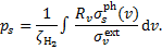
where p_s is an efficiency factor defined by $p_{s} = \frac{1}{ζ_{H_{2}}} \int \frac{R_{v} σ_{s}^{ph} (v)}{σ_{v}^{ext}} d v .$ ${p_s} = {1 \over {{\zeta _{{{\rm{H}}_2}}}}}\mathop \smallint \nolimits^ {{{R_v}\sigma _s^{{\rm{ph}}}(v)} \over {\sigma _v^{{\rm{ext}}}}}{\rm{d}}v.$ (A.8)

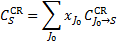
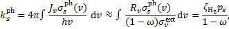
Therefore, the values of p_s tabulated by G89 can be compared to our values of $(1 - ω) k_{0, s}^{ph}$ $(1 - \omega )k_{0,s}^{{\rm{ph}}}$ .

Table A.1

CR excitation rates, $C_{s}^{CR}$ $C_s^{{\rm{CR}}}$ , normalised to the CR ionisation rate, $ζ_{H_{2}}$ ${\zeta _{{{\rm{H}}_2}}}$ .

Appendix B Update of cosmic-ray ionisation data

In Fig. B.1, we present the most-updated compilation of CR ionisation rate estimates obtained from observations in diffuse clouds, low- and high-mass star-forming regions, circumstellar discs, and massive hot cores (see also Padovani 2023). In the same plot we show the trend of $ζ_{H_{2}}$ ${\zeta _{{{\rm{H}}_2}}}$ predicted by CR propagation models (e.g. Padovani et al. 2009, 2018b, 2022) described in Sect. 3.1. Models also include the contribution of primary CR electrons and secondary electrons. We note that the models presented here only account for the propagation of interstellar CRs, but in more evolved sources, such as in high-mass star-forming regions and hot cores, there could be a substantial contribution from locally accelerated charged particles (Padovani et al. 2015, 2016; Gaches & Offner 2018; Padovani et al. 2021).

Below, we also present polynomial fits of the three trends of $ζ_{H_{2}}$ ${\zeta _{{{\rm{H}}_2}}}$ predicted by the models. These parameterisations differ from those presented in Padovani et al. (2018b) as here we take into account the rigorous calculation of secondary electrons presented in Ivlev et al. (2021) in the regime of continuous slowing-down approximation (Takayanagi 1973; Padovani et al. 2009). The CR ionisation rate can be parameterised with the following fitting formula: 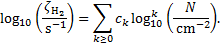$\log_{10} (\frac{ζ_{H_{2}}}{s^{- 1}}) = \sum_{k \geq 0} c_{k} \log_{10}^{k} (\frac{N}{{cm}^{- 2}}) .$ ${\log _{10}}\left( {{{{\zeta _{{{\rm{H}}_2}}}} \over {{{\rm{s}}^{ - 1}}}}} \right) = \mathop \sum \limits_{k \ge 0} {c_k}\log _{10}^k\left( {{N \over {{\rm{c}}{{\rm{m}}^{ - 2}}}}} \right).$ (B.1)

Equation (B.1) is valid for 10¹⁹ ≤ N/cm⁻² ≤ 10²⁵. The coefficients c_k are given in Table B.1.

Table B.1

Coefficients c_k of the polynomial fit, Eq. (B.1).

Fig. B.1

Total CR ionisation rate as a function of the H₂ column density. Theoretical models ℒ (lower solid black line), ℋ (dotted black line), and 𝓤 (upper solid black line). Expected values from models also include the ionisation due to primary CR electrons and secondary electrons. Observational estimates in diffuse clouds: solid down-pointing triangle (Shaw et al. 2008), solid up-pointing triangle (Neufeld et al. 2010), solid left-pointing triangles (Indriolo & McCall 2012), solid right-pointing triangles (Neufeld & Wolfire 2017), empty right-pointing triangles (Luo et al. 2023a), empty left-pointing triangles (Luo et al. 2023b); in low-mass dense cores: solid circles (Caselli et al. 1998), empty hexagons (Bialy et al. 2022), empty circle (Maret & Bergin 2007), empty pentagon (Fuente et al. 2016), empty up-pointing triangle (Redaelli et al. 2021); in high-mass star-forming regions: stars (Sabatini et al. 2020), black and grey small symbols (Sabatini et al. 2023), solid diamonds (de Boisanger et al. 1996), empty diamonds (van der Tak et al. 2000), empty thin diamonds (Hezareh et al. 2008), solid thin diamonds (Morales Ortiz et al. 2014); in circumstellar discs: empty squares (Cec-carelli et al. 2004); in massive hot cores: solid squares (Barger & Garrod 2020).

Appendix C Updated energy loss functions

The quantity that governs the decrease in energy of a particle as it moves through a medium is referred to as the energy loss function. For electrons colliding with H₂ molecules, the energy loss function is given by $\begin{array}{l} L_{e} (E) = L_{e}^{C} (E) \frac{2 m_{e}}{m_{H_{2}}} σ_{e}^{mt . t} (E) E + \sum_{j} σ_{e}^{exc, j} (E) E_{thr, j} \\ + \int_{0}^{(E - I) / 2} \frac{d σ_{e}^{H_{2}} (E, ε)}{d ε} (I + ε) d ε \\ + \int_{0}^{E} \frac{d σ_{e}^{br} (E, E_{γ})}{d E_{γ}} E_{γ} d E_{γ} + K E^{2} \end{array}$ $\eqalign{ & {L_e}(E) = L_e^{\rm{C}}(E){{2{m_e}} \over {{m_{{{\rm{H}}_2}}}}}\sigma _e^{{\rm{m}}.{\rm{t}}}(E)E + \sum\limits_j {\sigma _e^{{\rm{exc}},j}} (E){E_{{\rm{thr}},j}} \cr & \,\,\,\,\,\,\,\,\,\,\,\,\,\, + \int_0^{(E - I)/2} {{{{\rm{d}}\sigma _e^{{{\rm{H}}_2}}(E,\varepsilon )} \over {{\rm{d}}\varepsilon }}} (I + \varepsilon ){\rm{d}}\varepsilon \cr & \,\,\,\,\,\,\,\,\,\,\,\, + \int_0^E {{{{\rm{d}}\sigma _e^{{\rm{br}}}\left( {E,{E_\gamma }} \right)} \over {{\rm{d}}{E_\gamma }}}} {E_\gamma }{\rm{d}}{E_\gamma } + K{E^2}. \cr}$ (C.1)

The terms on the right-hand side are momentum transfer, rotational and vibrational excitation, electronic excitation, ionisa-tion, bremsstrahlung, and synchrotron losses. Here, m_e and $m_{H_{2}}$ ${m_{{H_2}}}$ denote the mass of the electron and H₂, respectively, $σ_{e}^{m . t .}$ $\sigma _e^{{\rm{m}}.{\rm{t}}.}$ · and $σ_{e}^{exc, k}$ $\sigma _e^{{\rm{exc}},k}$ are the cross sections of momentum transfer and excitation of state k, E_thr,k is the corresponding threshold energy of the excitation, $d σ_{e}^{H_{2}} / d ε$ ${\rm{d}}\sigma _e^{{{\rm{H}}_2}}/{\rm{d}}\varepsilon$ is the differential ionisation cross section (Kim et al. 2000), where ɛ is the energy of the secondary electron and I = 15.43 eV is the ionisation threshold, $d σ_{e}^{br} / d E_{γ}$ ${\rm{d}}\sigma _e^{{\rm{br}}}/{\rm{d}}{E_\gamma }$ is the bremsstrahlung differential cross section (Blumenthal & Gould 1970), where E_γ is the energy of the emitted photon, and KE² represents synchrotron losses with K = 5 × 10⁻³⁸ eV cm² and E in eV (Schlickeiser 2002). We assume the relationship by Crutcher (2012) between the magnetic field strength, B, and the volume density, n, B = B₀(n/n₀)^κ, with B₀ = 10 µG, n₀ = 150 cm⁻³, and κ = 0.5-0.7. Choosing κ = 0.5 removes the dependence on volume density (see Padovani et al. 2018b, for details). Depending on the ionisation fraction and the temperature of the medium, Coulomb losses, $L_{e}^{C} (E)$ $L_e^{\rm{C}}(E)$ , must be also included (Swartz et al. 1971).

Similarly, for protons colliding with H₂, the energy loss function is given by $\begin{array}{l} L_{p} (E) = L_{p}^{C} (E) + \frac{2 m_{p} m_{H_{2}}}{{(m_{p} + m_{H_{2}})}^{2}} σ_{p}^{m . t} (E) E + \sum_{j} σ_{p}^{exc, j} (E) E_{thr, j} \\ + (I + 〈 ε 〉) \frac{σ_{p}^{e.c.} σ_{H}^{self-ion}}{σ_{p}^{e.c.} + σ_{H}^{self-ion}} \\ + \int_{0}^{4 m_{e} E / m_{p}} \frac{d σ_{p}^{H_{2}} (E, ε)}{d ε} (I + ε) d ε + L_{p}^{π} (E) \end{array}$ $\eqalign{ & {L_p}(E) = L_p^{\rm{C}}(E) + {{2{m_p}{m_{{{\rm{H}}_2}}}} \over {{{\left( {{m_p} + {m_{{{\rm{H}}_2}}}} \right)}^2}}}\sigma _p^{{\rm{m}}.{\rm{t}}}(E)E + \sum\limits_j {\sigma _p^{{\rm{exc}},j}} (E){E_{{\rm{thr}},j}} \cr & \,\,\,\,\,\,\,\,\,\,\,\,\,\,\,\, + (I + \langle \varepsilon \rangle ){{\sigma _p^{{\rm{e}}{\rm{.c}}{\rm{. }}}\sigma _{\rm{H}}^{{\rm{self - ion }}}} \over {\sigma _p^{{\rm{e}}{\rm{.c}}{\rm{. }}} + \sigma _{\rm{H}}^{{\rm{self - ion }}}}} \cr & \,\,\,\,\,\,\,\,\,\,\,\,\,\,\, + \int_0^{4{m_e}E/{m_p}} {{{{\rm{d}}\sigma _p^{{{\rm{H}}_2}}(E,\varepsilon )} \over {{\rm{d}}\varepsilon }}} (I + \varepsilon ){\rm{d}}\varepsilon + L_p^\pi (E) \cr}$ (C.2)

In addition to the momentum transfer, excitation, and ionisation terms described in Eq. (C.1) for the electron energy loss function, on the right-hand side there are losses due to electron capture (term in the second row of Eq. C.2) and pion production (last term of Eq. C.2).

Energy losses by electron capture can be derived following the methodology presented in the works by Edgar et al. (1973); Miller & Green (1973); Edgar et al. (1975). The following cycle must be considered: $\begin{array}{l} p + H_{2} \to H_{fast} + H_{2}^{+} \\ H_{fast} + H_{2} \to p + H_{2} + e^{-} \end{array}$ $\matrix{ {p + {{\rm{H}}_2} \to {{\rm{H}}_{{\rm{fast}}}} + {\rm{H}}_2^ + } \hfill \cr {{{\rm{H}}_{{\rm{fast}}}} + {{\rm{H}}_2} \to p + {{\rm{H}}_2} + {e^ - }} \hfill \cr }$

During the first process, the ionisation energy of H₂ is lost, and in the second process the average energy of the ejected electron, 〈ɛ〉, is lost. Thus, the net contribution of the electron capture cycle to the loss function is $L_{p}^{e.c.} = f_{p} I σ_{p}^{e.c.} + f_{H} 〈 ε 〉 σ_{H}^{self-1on},$ $L_p^{{\rm{e}}{\rm{.c}}{\rm{.}}} = {f_p}I\sigma _p^{{\rm{e}}{\rm{.c}}{\rm{.}}} + {f_{\rm{H}}}\langle \varepsilon \rangle \sigma _{\rm{H}}^{{\rm{self - 1on}}},$ (C.3)

where $f_{H} = \frac{σ_{p}^{e.c.}}{σ_{p}^{e.c.} + σ_{H}^{self - ion}}$ ${f_{\rm{H}}} = {{\sigma _p^{{\rm{e}}{\rm{.c}}{\rm{.}}}} \over {\sigma _p^{{\rm{e}}{\rm{.c}}{\rm{.}}} + \sigma _{\rm{H}}^{{\rm{self}} - {\rm{ion}}}}}$ (C.4)

and f_p = 1 − ƒ_H. Here $σ_{p}^{e.c.}$ $\sigma _p^{{\rm{e}}{\rm{.c}}{\rm{.}}}$ ^. is the electon capture cross section (Gilbody & Hasted 1957; Curran et al. 1959; De Heer et al. 1966; Toburen & Wilson 1972; Rudd et al. 1983; Gealy & van Zyl 1987; Baer et al. 1988; Phelps 1990; Errea et al. 2010), $σ_{H}^{self-ion}$ $\sigma _{\rm{H}}^{{\rm{self - ion}}}$ is the self-ionisation of hydrogen atoms (Stier & Barnett 1956; van Zyl et al. 1981; Phelps 1990), and $〈 ε 〉 = ε_{0} - \frac{ε_{\max}}{\exp (ε_{\max} / ε_{0}) - 1},$ $\langle \varepsilon \rangle = {\varepsilon _0} - {{{\varepsilon _{\max }}} \over {\exp \left( {{\varepsilon _{\max }}/{\varepsilon _0}} \right) - 1}},$ (C.5)

where ɛ_max = 4(m_e/m_p)E is the maximum energy of the ejected secondary electron corresponding to an incident proton of energy E, and ɛ₀ is the saturation energy of the secondary electron, adjusted to reproduce the experimental data, which is set to 20 eV. Finally, the expression for Coulomb losses, $L_{p}^{C} (E)$ $L_p^{\rm{C}}(E)$ , is given by Mannheim & Schlickeiser (1994) and for pion losses, $L_{p}^{π}$ $L_p^\pi$ , whose contribution dominates above 280 MeV is given by Krakau & Schlickeiser (2015).

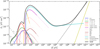Fig. C.1

Energy loss function for electrons colliding with H₂ (solid black line). Coloured lines show the different components and the following references point to the papers from which the relative cross sections have been adopted: momentum transfer (‘m.t.’, solid blue; Pinto & Galli 2008); the rotational transition J = 0 → 2 (solid green line; England et al. 1988); vibrational transitions v = 0 → 1 (solid red line; Yoon et al. 2008) and v = 0 → 2 (dashed red line; Janev et al. 2003); electronic transitions summed over all the triplet and singlet states (solid orange and magenta lines, respectively; Scarlett et al. 2021); Lyman series (solid pink lines; van Zyl et al. 1989; Ajello et al. 1991, 1996); Balmer series (solid brown lines; Möhlmann et al. 1977; Karolis & Harting 1978; Williams et al. 1982); ionisation (solid cyan line; Kim et al. 2000); bremsstrahlung (solid grey line; Blumenthal & Gould 1970; Padovani et al. 2018a); and synchrotron (solid yellow line; Schlickeiser 2002). Dash-dotted grey lines show the Coulomb losses at 10 K for ionisation fractions equal to 10⁻⁷ and 10⁻⁸ (Swartz et al. 1971) and the solid yellow line shows the synchrotron losses (Schlickeiser 2002).

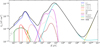Fig. C.2

Energy loss function for protons colliding with H₂ (solid black line). Coloured lines show the different components and the following references point to the papers from which the relative cross sections have been adopted: momentum transfer (‘m.t.’, solid blue; Pinto & Galli 2008); the rotational transition J = 0 → 2 (solid green line; Gianturco & Tritella 1977; Linder 1980); vibrational transitions v = 0 → 1 and v = 0 → 2 (solid and dashed red lines, respectively; Gentry & Giese 1975; Herrero & Doering 1972; Schinke 1977; Niedner et al. 1987; Janev et al. 2003); dissociation (solid orange line; Janev et al. 2003); Lyα (solid pink line; van Zyl et al. 1967, 1989; Phelps 1990); Hα (solid brown line; Williams et al. 1982); electron capture (solid purple line; Gilbody & Hasted 1957; Curran et al. 1959; De Heer et al. 1966; Toburen & Wilson 1972; Rudd et al. 1983; Gealy & van Zyl 1987; Baer et al. 1988; Phelps 1990; Errea et al. 2010); ionisation (solid cyan line; Rudd 1988; Krause et al. 2015); and pion production (solid yellow line; Krakau & Schlickeiser 2015). Dash-dotted grey lines show the Coulomb losses at 10 K for an ionisation fraction of 10⁻⁷ (Mannheim & Schlickeiser 1994).

Appendix D Photorates for various R_V values

Table D.1

Photodissociation rates normalised to the CR ionisation rate, $k_{0, s}^{pd}$ $k_{0,s}^{{\rm{pd}}}$ , for H₂ o:p=0:1 and H₂ o:p=1:0 and for R_V = 3.1.

Table D.2

Photoionisation rates normalised to the CR ionisation rate, $k_{0, s}^{pi}$ $k_{0,s}^{{\rm{pi}}}$ , for H₂ o:p=0:1 and H₂ o:p=1:0 and for R_v = 3.1.

Table D.3

Same as Table D.1, but for R_V = 4.0.

Table D.4

Same as Table D.2, but for R_v = 4.0.

Table D.5

Same as Table D.1, but for R_v = 5.5.

Table D.6

Same as Table D.2, but for R_V = 5.5.

References

Abgrall, H., Roueff, E., Launay, F., Roncin, J. Y., & Subtil, J. L. 1993a, A&AS, 101, 273 [NASA ADS] [Google Scholar]
Abgrall, H., Roueff, E., Launay, F., Roncin, J. Y., & Subtil, J. L. 1993b, A&AS, 101, 323 [NASA ADS] [Google Scholar]
Abgrall, H., Roueff, E., Launay, F., Roncin, J. Y., & Subtil, J. L. 1993c, J. Mol. Spectrosc., 157, 512 [NASA ADS] [CrossRef] [Google Scholar]
Abgrall, H., Roueff, E., Liu, X., & Shemansky, D. E. 1997, ApJ, 481, 557 [NASA ADS] [CrossRef] [Google Scholar]
Abgrall, H., Roueff, E., & Drira, I. 2000, A&AS, 141, 297 [NASA ADS] [CrossRef] [EDP Sciences] [Google Scholar]
Ajello, J. M., Shemansky, D. E., & James, G. K. 1991, ApJ, 371, 422 [NASA ADS] [CrossRef] [Google Scholar]
Ajello, J. M., Ahmed, S. M., & Liu, X. 1996, Phys. Rev. A, 53, 2303 [NASA ADS] [CrossRef] [Google Scholar]
Baer, M., Niedner, G., & Toennies, J. P. 1988, J. Chem. Phys., 88, 1461 [NASA ADS] [CrossRef] [Google Scholar]
Barger, C. J., & Garrod, R. T. 2020, ApJ, 888, 38 [Google Scholar]
Bialy, S. 2020, Commun. Phys., 3, 32 [NASA ADS] [CrossRef] [Google Scholar]
Bialy, S., Belli, S., & Padovani, M. 2022, A&A, 658, A13 [Google Scholar]
Bieri, G., Schmelzer, A., Åsbrink, L., & Jonsson, M. 1980, Chem. Phys., 49, 213 [NASA ADS] [CrossRef] [Google Scholar]
Blumenthal, G. R., & Gould, R. J. 1970, Rev. Mod. Phys., 42, 237 [Google Scholar]
Bohlin, R. C., Savage, B. D., & Drake, J. F. 1978, ApJ, 224, 132 [Google Scholar]
Caselli, P., & Ceccarelli, C. 2012, A&ARv, 20, 56 [Google Scholar]
Caselli, P., Walmsley, C. M., Terzieva, R., & Herbst, E. 1998, ApJ, 499, 234 [Google Scholar]
Ceccarelli, C., Dominik, C., Lefloch, B., Caselli, P., & Caux, E. 2004, ApJ, 607, L51 [NASA ADS] [CrossRef] [Google Scholar]
Cecchi-Pestellini, C., & Aiello, S. 1992, MNRAS, 258, 125 [NASA ADS] [CrossRef] [Google Scholar]
Crutcher, R. M. 2012, ARA&A, 50, 29 [Google Scholar]
Curran, R., Donahue, T. M., & Kasner, W. H. 1959, Phys. Rev., 114, 490 [NASA ADS] [CrossRef] [Google Scholar]
Dahlberg, D. A., Anderson, D. K., & Dayton, I. E. 1968, Phys. Rev., 170, 127 [NASA ADS] [CrossRef] [Google Scholar]
de Boisanger, C., Helmich, F. P., & van Dishoeck, E. F. 1996, A&A, 310, 315 [NASA ADS] [Google Scholar]
De Heer, F. J., Schutten, J., & Moustafa, H. 1966, Physica, 32, 1766 [NASA ADS] [CrossRef] [Google Scholar]
Draine, B. T. 1978, ApJS, 36, 595 [Google Scholar]
Draine, B. T. 2003a, ARA&A, 41, 241 [NASA ADS] [CrossRef] [Google Scholar]
Draine, B. T. 2003b, ApJ, 598, 1017 [NASA ADS] [CrossRef] [Google Scholar]
Draine, B. T. 2003c, ApJ, 598, 1026 [Google Scholar]
Drozdowski, R., & Kowalski, A. 2018, Eur. Phys. J. D, 72, 220 [NASA ADS] [CrossRef] [Google Scholar]
Edgar, B. C., Miles, W. T., & Green, A. E. S. 1973, J. Geophys. Res., 78, 6595 [NASA ADS] [CrossRef] [Google Scholar]
Edgar, B. C., Porter, H. S., & Green, A. E. S. 1975, Planet. Space Sci., 23, 787 [NASA ADS] [CrossRef] [Google Scholar]
Edwards, J. L., & Thomas, E. W. 1968, Phys. Rev., 165, 16 [NASA ADS] [CrossRef] [Google Scholar]
England, J. P., Elford, M. T., & Crompton, R. W. 1988, Austr. J. Phys., 41, 573 [NASA ADS] [CrossRef] [Google Scholar]
Errea, L. F., Illescas, C., Macías, A., et al. 2010, J. Chem. Phys., 133, 244307 [NASA ADS] [CrossRef] [Google Scholar]
Fedoseev, G., Ioppolo, S., & Linnartz, H. 2015, MNRAS, 446, 449 [NASA ADS] [CrossRef] [Google Scholar]
Flower, D. R., & Watt, G. D. 1984, MNRAS, 209, 25 [NASA ADS] [Google Scholar]
Fuente, A., Cernicharo, J., Roueff, E., et al. 2016, A&A, 593, A94 [NASA ADS] [CrossRef] [EDP Sciences] [Google Scholar]
Gaches, B. A. L., & Offner, S. S. R. 2018, ApJ, 861, 87 [NASA ADS] [CrossRef] [Google Scholar]
Gealy, M. W., & van Zyl, B. 1987, Phys. Rev. A, 36, 3100 [NASA ADS] [CrossRef] [Google Scholar]
Gentry, W. R., & Giese, C. F. 1975, Phys. Rev. A, 11, 90 [NASA ADS] [CrossRef] [Google Scholar]
Gianturco, F. A., & Tritella, P. 1977, Phys. Rev. A, 16, 542 [NASA ADS] [CrossRef] [Google Scholar]
Gilbody, H. B., & Hasted, J. B. 1957, Proc. Roy. Soc. Lond. Ser. A, 240, 382 [NASA ADS] [CrossRef] [Google Scholar]
Gredel, R., & Dalgarno, A. 1995, ApJ, 446, 852 [NASA ADS] [CrossRef] [Google Scholar]
Gredel, R., Lepp, S., & Dalgarno, A. 1987, ApJ, 323, L137 [Google Scholar]
Gredel, R., Lepp, S., Dalgarno, A., & Herbst, E. 1989, ApJ, 347, 289 [Google Scholar]
Heays, A. N., Bosman, A. D., & van Dishoeck, E. F. 2017, A&A, 602, A105 [NASA ADS] [CrossRef] [EDP Sciences] [Google Scholar]
Hernández, M. I., Tejeda, G., Fernández, J. M., & Montero, S. 2021, A&A, 647, A155 [NASA ADS] [CrossRef] [EDP Sciences] [Google Scholar]
Herrero, F. A., & Doering, J. P. 1972, Phys. Rev. A, 5, 702 [NASA ADS] [CrossRef] [Google Scholar]
Hezareh, T., Houde, M., McCoey, C., Vastel, C., & Peng, R. 2008, ApJ, 684, 1221 [NASA ADS] [CrossRef] [Google Scholar]
Hiraoka, K., Yamashita, A., Yachi, Y., et al. 1995, ApJ, 443, 363 [NASA ADS] [CrossRef] [Google Scholar]
Hrodmarsson, H. R., & van Dishoeck, E. F. 2023, A&A, 675, A25 [NASA ADS] [CrossRef] [EDP Sciences] [Google Scholar]
Ibáñez-Mejía, J. C., Walch, S., Ivlev, A. V., et al. 2019, MNRAS, 485, 1220 [CrossRef] [Google Scholar]
Indriolo, N., & McCall, B. J. 2012, ApJ, 745, 91 [NASA ADS] [CrossRef] [Google Scholar]
Ivlev, A. V., Padovani, M., Galli, D., & Caselli, P. 2015, ApJ, 812, 135 [Google Scholar]
Ivlev, A. V., Silsbee, K., Padovani, M., & Galli, D. 2021, ApJ, 909, 107 [NASA ADS] [CrossRef] [Google Scholar]
Janev, R. K., Reiter, D., & Samm, U. 2003, Collision Processes in Low-Temperature Hydrogen Plasmas (Jülich, Germany: Forschungszentrum, Zentralbibliothek) [Google Scholar]
Karolis, C., & Harting, E. 1978, J. Phys. B At. Mol. Phys., 11, 357 [NASA ADS] [CrossRef] [Google Scholar]
Kim, Y.-K., Santos, J. P., & Parente, F. 2000, Phys. Rev. A, 62, 052710 [NASA ADS] [CrossRef] [Google Scholar]
Krakau, S., & Schlickeiser, R. 2015, ApJ, 802, 114 [NASA ADS] [CrossRef] [Google Scholar]
Kramida, A., Ralchenko, Yu., Reader, J., & and NIST ASD Team 2022, NIST Atomic Spectra Database (ver. 5.10), Available: https://physics.nist.gov/asd (Gaithersburg, MD: National Institute of Standards and Technology) [Google Scholar]
Krause, J., Morlino, G., & Gabici, S. 2015, 34th International Cosmic Ray Conference (ICRC2015), 518 [Google Scholar]
Li, A., & Draine, B. T. 2001, ApJ, 554, 778 [Google Scholar]
Linder, F. 1980, in Proceedings of the XIth International Conference on the Physics of Electronic and Atomic Collisions, eds. N. Oda, & L. Takayanagi, 535 [Google Scholar]
Liu, X., Johnson, P. V., Malone, C. P., et al. 2010, ApJ, 716, 701 [NASA ADS] [CrossRef] [Google Scholar]
Luo, G., Zhang, Z.-Y., Bisbas, T. G., et al. 2023a, ApJ, 942, 101 [NASA ADS] [CrossRef] [Google Scholar]
Luo, G., Zhang, Z.-Y., Bisbas, T. G., et al. 2023b, ApJ, 946, 91 [NASA ADS] [CrossRef] [Google Scholar]
Mannheim, K., & Schlickeiser, R. 1994, A&A, 286, 983 [NASA ADS] [Google Scholar]
Maret, S., & Bergin, E. A. 2007, ApJ, 664, 956 [Google Scholar]
Mark, J. C. 1944, The spherical harmonic method. I (National Research Council of Canada, Atomic Energy Project, Report MT 92) [Google Scholar]
Mark, J. C. 1945, The spherical harmonic method. II (National Research Council of Canada, Atomic Energy Project, Report MT 97) [Google Scholar]
Miller, J. H., & Green, A. E. S. 1973, Radiat. Res., 54, 343 [NASA ADS] [CrossRef] [Google Scholar]
Möhlmann, G. R., De Heer, F. J., & Los, J. 1977, Chem. Phys., 25, 103 [CrossRef] [Google Scholar]
Morales Ortiz, J. L., Ceccarelli, C., Lis, D. C., et al. 2014, A&A, 563, A127 [NASA ADS] [CrossRef] [EDP Sciences] [Google Scholar]
Neufeld, D. A., & Wolfire, M. G. 2017, ApJ, 845, 163 [Google Scholar]
Neufeld, D. A., Goicoechea, J. R., Sonnentrucker, P., et al. 2010, A&A, 521, A10 [Google Scholar]
Niedner, G., Noll, M., Toennies, J. P., & Schlier, C. 1987, J. Chem. Phys., 87, 2685 [NASA ADS] [CrossRef] [Google Scholar]
Padovani, M. 2023, in Physics and Chemistry of Star Formation: The Dynamical ISM Across Time and Spatial Scales, 237 [Google Scholar]
Padovani, M., Galli, D., & Glassgold, A. E. 2009, A&A, 501, 619 [NASA ADS] [CrossRef] [EDP Sciences] [Google Scholar]
Padovani, M., Hennebelle, P., Marcowith, A., & Ferrière, K. 2015, A&A, 582, A13 [Google Scholar]
Padovani, M., Marcowith, A., Hennebelle, P., & Ferrière, K. 2016, A&A, 590, A8 [NASA ADS] [CrossRef] [EDP Sciences] [Google Scholar]
Padovani, M., Galli, D., Ivlev, A. V., Caselli, P., & Ferrara, A. 2018a, A&A, 619, A144 [NASA ADS] [CrossRef] [EDP Sciences] [Google Scholar]
Padovani, M., Ivlev, A. V., Galli, D., & Caselli, P. 2018b, A&A, 614, A111 [NASA ADS] [CrossRef] [EDP Sciences] [Google Scholar]
Padovani, M., Marcowith, A., Galli, D., Hunt, L. K., & Fontani, F. 2021, A&A, 649, A149 [NASA ADS] [CrossRef] [EDP Sciences] [Google Scholar]
Padovani, M., Bialy, S., Galli, D., et al. 2022, A&A, 658, A189 [NASA ADS] [CrossRef] [EDP Sciences] [Google Scholar]
Phelps, A. V. 1990, J. Phys. Chem. Ref. Data, 19, 653 [NASA ADS] [CrossRef] [Google Scholar]
Pinto, C., & Galli, D. 2008, A&A, 484, 17 [NASA ADS] [CrossRef] [EDP Sciences] [Google Scholar]
Prasad, S. S., & Tarafdar, S. P. 1983, ApJ, 267, 603 [Google Scholar]
Redaelli, E., Sipilä, O., Padovani, M., et al. 2021, A&A, 656, A109 [NASA ADS] [CrossRef] [EDP Sciences] [Google Scholar]
Roberge, W. G. 1983, ApJ, 275, 292 [CrossRef] [Google Scholar]
Roueff, E., Abgrall, H., Czachorowski, P., et al. 2019, A&A, 630, A58 [NASA ADS] [CrossRef] [EDP Sciences] [Google Scholar]
Rudd, M. E. 1988, Phys. Rev. A, 38, 6129 [NASA ADS] [CrossRef] [Google Scholar]
Rudd, M. E., Goffe, T. V., Dubois, R. D., Toburen, L. H., & Ratcliffe, C. A. 1983, Phys. Rev. A, 28, 3244 [NASA ADS] [CrossRef] [Google Scholar]
Sabatini, G., Bovino, S., Giannetti, A., et al. 2020, A&A, 644, A34 [EDP Sciences] [Google Scholar]
Sabatini, G., Bovino, S., & Redaelli, E. 2023, ApJ, 947, L18 [NASA ADS] [CrossRef] [Google Scholar]
Scarlett, L. H., Fursa, D. V., Zammit, M. C., et al. 2021, At. Data Nucl. Data Tables, 137, 101361 [NASA ADS] [CrossRef] [Google Scholar]
Scarlett, L. H., Rehill, U. S., Zammit, M. C., et al. 2023, Phys. Rev. A, 107, 062804 [NASA ADS] [CrossRef] [Google Scholar]
Schinke, R. 1977, Chem. Phys., 24, 379 [NASA ADS] [CrossRef] [Google Scholar]
Schlickeiser, R. 2002, Cosmic Ray Astrophysics (Berlin: Springer) [CrossRef] [Google Scholar]
Shaw, G., Ferland, G. J., Srianand, R., et al. 2008, ApJ, 675, 405 [NASA ADS] [CrossRef] [Google Scholar]
Shemansky, D. E., Ajello, J. M., & Hall, D. T. 1985, ApJ, 296, 765 [NASA ADS] [CrossRef] [Google Scholar]
Shen, C. J., Greenberg, J. M., Schutte, W. A., & van Dishoeck, E. F. 2004, A&A, 415, 203 [NASA ADS] [CrossRef] [EDP Sciences] [Google Scholar]
Shiner, D., Gilligan, J. M., Cook, B. M., & Lichten, W. 1993, Phys. Rev. A, 47, 4042 [NASA ADS] [CrossRef] [Google Scholar]
Sternberg, A., Dalgarno, A., & Lepp, S. 1987, ApJ, 320, 676 [NASA ADS] [CrossRef] [Google Scholar]
Stier, P. M., & Barnett, C. F. 1956, Phys. Rev., 103, 896 [NASA ADS] [CrossRef] [Google Scholar]
Swartz, W. E., Nisbet, J. S., & Green, A. E. S. 1971, J. Geophys. Res., 76, 8425 [NASA ADS] [CrossRef] [Google Scholar]
Takayanagi, K. 1973, PASJ, 25, 327 [NASA ADS] [Google Scholar]
Thomas, E. W. 1972, Excitation in Heavy Particle Collisions (New York: Wiley-Interscience) [Google Scholar]
Tielens, A. G. G. M., & Hagen, W. 1982, A&A, 114, 245 [Google Scholar]
Toburen, L. H., & Wilson, W. E. 1972, Phys. Rev. A, 5, 247 [NASA ADS] [CrossRef] [Google Scholar]
Trickl, T., Cromwell, E. F., Lee, Y. T., & Kung, A. H. 1989, J. Chem. Phys., 91, 6006 [NASA ADS] [CrossRef] [Google Scholar]
van der Tak, F. F. S., van Dishoeck, E. F., Evans, Neal J., I., & Blake, G. A. 2000, ApJ, 537, 283 [Google Scholar]
van Dishoeck, E. F., & Black, J. H. 1982, ApJ, 258, 533 [NASA ADS] [CrossRef] [Google Scholar]
van Zyl, B., Jaecks, D., Pretzer, D., & Geballe, R. 1967, Phys. Rev., 158, 29 [NASA ADS] [CrossRef] [Google Scholar]
van Zyl, B., Le, T. Q., & Amme, R. C. 1981, J. Chem. Phys., 74, 314 [NASA ADS] [CrossRef] [Google Scholar]
van Zyl, B., Gealy, M. W., & Neumann, H. 1989, Phys. Rev. A, 40, 1664 [NASA ADS] [CrossRef] [Google Scholar]
Weingartner, J. C., & Draine, B. T. 2001, ApJS, 134, 263 [CrossRef] [Google Scholar]
Williams, I. D., Geddes, J., & Gilbody, H. B. 1982, J. Phys. B At. Mol. Phys., 15, 1377 [NASA ADS] [CrossRef] [Google Scholar]
Yoon, J.-S., Song, M.-Y., Han, J.-M., et al. 2008, J. Phys. Chem. Ref. Data, 37, 913 [CrossRef] [Google Scholar]
Zammit, M. C., Fursa, D. V., Savage, J. S., & Bray, I. 2017a, J. Phys. B At. Mol. Opt. Phys., 50, 123001 [NASA ADS] [CrossRef] [Google Scholar]
Zammit, M. C., Savage, J. S., Fursa, D. V., & Bray, I. 2017b, Phys. Rev. A, 95, 022708 [NASA ADS] [CrossRef] [Google Scholar]

¹

In this paper $ζ_{H_{2}}$ ${\zeta _{{{\rm{H}}_2}}}$ is the rate of production of $H_{2}^{+}$ ${\rm{H}}_2^ +$ ions per H₂ molecule. The dissociative ionisation and double ionisation of H₂, which produce H⁺ ions, are not considered here (for these processes, see Padovani et al. 2009).

²

All Tables

Table 1

Parameters of the Galactic CR electron and proton spectra, Eq. (7).

In the text

Table A.1

CR excitation rates, $C_{s}^{CR}$ $C_s^{{\rm{CR}}}$ , normalised to the CR ionisation rate, $ζ_{H_{2}}$ ${\zeta _{{{\rm{H}}_2}}}$ .

In the text

Table B.1

Coefficients c_k of the polynomial fit, Eq. (B.1).

In the text

Table D.1

Photodissociation rates normalised to the CR ionisation rate, $k_{0, s}^{pd}$ $k_{0,s}^{{\rm{pd}}}$ , for H₂ o:p=0:1 and H₂ o:p=1:0 and for R_V = 3.1.

In the text

Table D.2

Photoionisation rates normalised to the CR ionisation rate, $k_{0, s}^{pi}$ $k_{0,s}^{{\rm{pi}}}$ , for H₂ o:p=0:1 and H₂ o:p=1:0 and for R_v = 3.1.

In the text

Table D.3

Same as Table D.1, but for R_V = 4.0.

In the text

Table D.4

Same as Table D.2, but for R_v = 4.0.

In the text

Table D.5

Same as Table D.1, but for R_v = 5.5.

In the text

Table D.6

Same as Table D.2, but for R_V = 5.5.

In the text

All Figures

Fig. 1

Secondary-electron spectra compared to some electron excitation cross sections for singlet B, C, B′, and D and triplet a states as a function of the energy (Scarlett et al. 2023). The green-scale shaded regions enclose the secondary-electron spectra calculated at N = 10²⁰ cm⁻² (upper boundary) and 10²⁴ cm⁻² (lower boundary) for the three Galactic CR proton models (ℒ, ℋ, 𝒰). The five cross sections shown in black solid lines are the strongest ones for the excitation of the B, C, B′, and D singlet states and the triplet a state from the ground state X(0, 0). The inset shows the electron excitation cross section of atomic hydrogen leading to Lyman and Balmer lines (Möhlmann et al. 1977; Karolis & Harting 1978; van Zyl et al. 1989; Ajello et al. 1991, 1996).

In the text

Fig. 2

Ratio between the e-H2 excitation rates summed over the initial and final rotational states and the CR ionisation rate for model ℋ and N = 10²⁰ cm⁻² as a function of the upper vibrational level, vu. Each subplot shows results for a different lower vibrational level, v_l. Solid green, violet, magenta, blue, and orange circles refer to the excitation of the B, C, B′, D, and a states from the ground state X, respectively. Empty black circles show a subset of previous estimates by Cecchi-Pestellini & Aiello (1992, see Sect. 3.5 for more details.)

In the text

	Fig. 3 Histograms of the ratio between collisional and radiative excitation rates, C^CR/C^rad, for five representative column densities, from 10²⁰ to 10²² cm⁻², for an interstellar UV field with χ = 1, R_V = 3.1, and model ℋ. The black dashed line shows where collisional and radiative processes equally contribute to excitation of H₂.
In the text

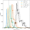	Fig. 4 Same as Fig. 3, but for models ℒ (thick lines) and 𝒰 (thin lines).
In the text

Fig. 5

Comparison of the optical depth, τ, of dust (black solid lines) to that of para- and ortho-H₂ (blue and cyan solid lines, respectively, upper-left panel), H (orange solid lines, upper-right panel), CO (green solid lines, bottom-left panel), and N₂ (purple solid lines, bottom-right panel) at N(H₂) = 10²¹ cm⁻². The H₂ optical depth is shown for model ℋ and H₂ o:p = 3:1. The H, CO, and N₂ optical depths have been computed by assuming constant abundances $(x_{H} = 10^{- 4}, x_{CO} = x_{N_{2}} = 10^{- 5})$ $\left( {{x_{\rm{H}}} = {{10}^{ - 4}},{x_{{\rm{CO}}}} = {x_{{{\rm{N}}_2}}} = } \right.{10^{ - 5}})$ and the photoabsorption cross sections presented in the Leiden Observatory database (https://home.strw.leidenuniv.nl/~ewine/photo/; see also Heays et al. 2017).

In the text

	Fig. 6 Mean intensity, J_V, of bound-bound H₂ transitions as a function of the wavelength, λ, for a molecular cloud with column density N = 10²³ cm⁻² illuminated by one side. Line spectra are shown separately for each excited electronic state. Results are shown for model ℋ , H₂ o:p=0:1, and R_V = 3.1.
In the text

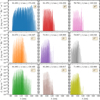	Fig. 7 Same as Fig. 6, but for H₂ o:p = 1:0.
In the text

Fig. 8

Mean intensity, J_v, of the continuum emission of H₂ from excited electronic states as a function of wavelength, λ, for a molecular cloud with a column density N = 10²³ cm⁻² illuminated by one side. The contribution of each excited electronic state (solid lines) is shown by solid coloured lines, while the dashed black line shows the total continuum emission. The inset shows the emission in the range 120–180 nm. Results are shown for model ℋ, H₂ o:p=0:1, and R_V = 3.1.

In the text

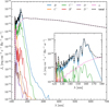	Fig. 9 Same as Fig. 8, but for H₂ o:p=1:0.
In the text

Fig. 10

Mean intensity, J_v, of the total emission in the wavelength range 72 < λ/nm < 250 for a molecular cloud illuminated by one side. From top to bottom the four panels show the expected mean intensity from H₂ lines, H₂ continuum, H lines (Lyα and Lyβ), and ISRF at four different column densities, from N = 10²¹ to 4 × 10²² cm⁻². Insets show the components of J_v at 400 < λ/nm < 700, highlighting three lines of the Balmer series (Hα, Hβ, and Hγ). Results are shown for model ℋ, χ = 1, H₂o:p=0:1, and R_v = 3.1.

In the text

Fig. 11

Photon fluxes, Φ_UV, as a function of the H₂ column density, N, below and above 180 nm (upper and lower panel, respectively) for χ = 1. Both panels show the integrated flux of CR-generated UV photons as a function of the three models of CR proton flux (ℒ, ℋ and 𝒰) and the ISRF UV flux. The cyan dotted lines show the integrated photon flux from H₂ and Η lines generated by collisional radiative excitation (labelled 'rad. exc.'). The three curves for each model correspond to R_V = 3.1 (lower curve), 4.0 (intermediate curve), and (5.5 upper curve). Arrows on the righthand side of the upper panel show previous estimates of Φ_UV, independent of column density: Prasad & Tarafdar (1983, PT83), Cecchi-Pestellini & Aiello (1992, CPA92), and Shen et al. (2004, S+04).

In the text

Fig. B.1

Total CR ionisation rate as a function of the H₂ column density. Theoretical models ℒ (lower solid black line), ℋ (dotted black line), and 𝓤 (upper solid black line). Expected values from models also include the ionisation due to primary CR electrons and secondary electrons. Observational estimates in diffuse clouds: solid down-pointing triangle (Shaw et al. 2008), solid up-pointing triangle (Neufeld et al. 2010), solid left-pointing triangles (Indriolo & McCall 2012), solid right-pointing triangles (Neufeld & Wolfire 2017), empty right-pointing triangles (Luo et al. 2023a), empty left-pointing triangles (Luo et al. 2023b); in low-mass dense cores: solid circles (Caselli et al. 1998), empty hexagons (Bialy et al. 2022), empty circle (Maret & Bergin 2007), empty pentagon (Fuente et al. 2016), empty up-pointing triangle (Redaelli et al. 2021); in high-mass star-forming regions: stars (Sabatini et al. 2020), black and grey small symbols (Sabatini et al. 2023), solid diamonds (de Boisanger et al. 1996), empty diamonds (van der Tak et al. 2000), empty thin diamonds (Hezareh et al. 2008), solid thin diamonds (Morales Ortiz et al. 2014); in circumstellar discs: empty squares (Cec-carelli et al. 2004); in massive hot cores: solid squares (Barger & Garrod 2020).

In the text

Fig. C.1

Energy loss function for electrons colliding with H₂ (solid black line). Coloured lines show the different components and the following references point to the papers from which the relative cross sections have been adopted: momentum transfer (‘m.t.’, solid blue; Pinto & Galli 2008); the rotational transition J = 0 → 2 (solid green line; England et al. 1988); vibrational transitions v = 0 → 1 (solid red line; Yoon et al. 2008) and v = 0 → 2 (dashed red line; Janev et al. 2003); electronic transitions summed over all the triplet and singlet states (solid orange and magenta lines, respectively; Scarlett et al. 2021); Lyman series (solid pink lines; van Zyl et al. 1989; Ajello et al. 1991, 1996); Balmer series (solid brown lines; Möhlmann et al. 1977; Karolis & Harting 1978; Williams et al. 1982); ionisation (solid cyan line; Kim et al. 2000); bremsstrahlung (solid grey line; Blumenthal & Gould 1970; Padovani et al. 2018a); and synchrotron (solid yellow line; Schlickeiser 2002). Dash-dotted grey lines show the Coulomb losses at 10 K for ionisation fractions equal to 10⁻⁷ and 10⁻⁸ (Swartz et al. 1971) and the solid yellow line shows the synchrotron losses (Schlickeiser 2002).

In the text

Fig. C.2

Energy loss function for protons colliding with H₂ (solid black line). Coloured lines show the different components and the following references point to the papers from which the relative cross sections have been adopted: momentum transfer (‘m.t.’, solid blue; Pinto & Galli 2008); the rotational transition J = 0 → 2 (solid green line; Gianturco & Tritella 1977; Linder 1980); vibrational transitions v = 0 → 1 and v = 0 → 2 (solid and dashed red lines, respectively; Gentry & Giese 1975; Herrero & Doering 1972; Schinke 1977; Niedner et al. 1987; Janev et al. 2003); dissociation (solid orange line; Janev et al. 2003); Lyα (solid pink line; van Zyl et al. 1967, 1989; Phelps 1990); Hα (solid brown line; Williams et al. 1982); electron capture (solid purple line; Gilbody & Hasted 1957; Curran et al. 1959; De Heer et al. 1966; Toburen & Wilson 1972; Rudd et al. 1983; Gealy & van Zyl 1987; Baer et al. 1988; Phelps 1990; Errea et al. 2010); ionisation (solid cyan line; Rudd 1988; Krause et al. 2015); and pion production (solid yellow line; Krakau & Schlickeiser 2015). Dash-dotted grey lines show the Coulomb losses at 10 K for an ionisation fraction of 10⁻⁷ (Mannheim & Schlickeiser 1994).

In the text

Current usage metrics show cumulative count of Article Views (full-text article views including HTML views, PDF and ePub downloads, according to the available data) and Abstracts Views on Vision4Press platform.

Data correspond to usage on the plateform after 2015. The current usage metrics is available 48-96 hours after online publication and is updated daily on week days.

Initial download of the metrics may take a while.

[1] Abgrall, H., Roueff, E., Launay, F., Roncin, J. Y., & Subtil, J. L. 1993a, A&AS, 101, 273 [NASA ADS] [Google Scholar]

[2] Abgrall, H., Roueff, E., Launay, F., Roncin, J. Y., & Subtil, J. L. 1993b, A&AS, 101, 323 [NASA ADS] [Google Scholar]

[3] Abgrall, H., Roueff, E., Launay, F., Roncin, J. Y., & Subtil, J. L. 1993c, J. Mol. Spectrosc., 157, 512 [NASA ADS] [CrossRef] [Google Scholar]

[4] Abgrall, H., Roueff, E., Liu, X., & Shemansky, D. E. 1997, ApJ, 481, 557 [NASA ADS] [CrossRef] [Google Scholar]

[5] Abgrall, H., Roueff, E., & Drira, I. 2000, A&AS, 141, 297 [NASA ADS] [CrossRef] [EDP Sciences] [Google Scholar]

[6] Ajello, J. M., Shemansky, D. E., & James, G. K. 1991, ApJ, 371, 422 [NASA ADS] [CrossRef] [Google Scholar]

[7] Ajello, J. M., Ahmed, S. M., & Liu, X. 1996, Phys. Rev. A, 53, 2303 [NASA ADS] [CrossRef] [Google Scholar]

[8] Baer, M., Niedner, G., & Toennies, J. P. 1988, J. Chem. Phys., 88, 1461 [NASA ADS] [CrossRef] [Google Scholar]

[9] Barger, C. J., & Garrod, R. T. 2020, ApJ, 888, 38 [Google Scholar]

[10] Bialy, S. 2020, Commun. Phys., 3, 32 [NASA ADS] [CrossRef] [Google Scholar]

[11] Bialy, S., Belli, S., & Padovani, M. 2022, A&A, 658, A13 [Google Scholar]

[12] Bieri, G., Schmelzer, A., Åsbrink, L., & Jonsson, M. 1980, Chem. Phys., 49, 213 [NASA ADS] [CrossRef] [Google Scholar]

[13] Blumenthal, G. R., & Gould, R. J. 1970, Rev. Mod. Phys., 42, 237 [Google Scholar]

[14] Bohlin, R. C., Savage, B. D., & Drake, J. F. 1978, ApJ, 224, 132 [Google Scholar]

[15] Caselli, P., & Ceccarelli, C. 2012, A&ARv, 20, 56 [Google Scholar]

[16] Caselli, P., Walmsley, C. M., Terzieva, R., & Herbst, E. 1998, ApJ, 499, 234 [Google Scholar]

[17] Ceccarelli, C., Dominik, C., Lefloch, B., Caselli, P., & Caux, E. 2004, ApJ, 607, L51 [NASA ADS] [CrossRef] [Google Scholar]

[18] Cecchi-Pestellini, C., & Aiello, S. 1992, MNRAS, 258, 125 [NASA ADS] [CrossRef] [Google Scholar]

[19] Crutcher, R. M. 2012, ARA&A, 50, 29 [Google Scholar]

[20] Curran, R., Donahue, T. M., & Kasner, W. H. 1959, Phys. Rev., 114, 490 [NASA ADS] [CrossRef] [Google Scholar]

[21] Dahlberg, D. A., Anderson, D. K., & Dayton, I. E. 1968, Phys. Rev., 170, 127 [NASA ADS] [CrossRef] [Google Scholar]

[22] de Boisanger, C., Helmich, F. P., & van Dishoeck, E. F. 1996, A&A, 310, 315 [NASA ADS] [Google Scholar]

[23] De Heer, F. J., Schutten, J., & Moustafa, H. 1966, Physica, 32, 1766 [NASA ADS] [CrossRef] [Google Scholar]

[24] Draine, B. T. 1978, ApJS, 36, 595 [Google Scholar]

[25] Draine, B. T. 2003a, ARA&A, 41, 241 [NASA ADS] [CrossRef] [Google Scholar]

[26] Draine, B. T. 2003b, ApJ, 598, 1017 [NASA ADS] [CrossRef] [Google Scholar]

[27] Draine, B. T. 2003c, ApJ, 598, 1026 [Google Scholar]

[28] Drozdowski, R., & Kowalski, A. 2018, Eur. Phys. J. D, 72, 220 [NASA ADS] [CrossRef] [Google Scholar]

[29] Edgar, B. C., Miles, W. T., & Green, A. E. S. 1973, J. Geophys. Res., 78, 6595 [NASA ADS] [CrossRef] [Google Scholar]

[30] Edgar, B. C., Porter, H. S., & Green, A. E. S. 1975, Planet. Space Sci., 23, 787 [NASA ADS] [CrossRef] [Google Scholar]

[31] Edwards, J. L., & Thomas, E. W. 1968, Phys. Rev., 165, 16 [NASA ADS] [CrossRef] [Google Scholar]

[32] England, J. P., Elford, M. T., & Crompton, R. W. 1988, Austr. J. Phys., 41, 573 [NASA ADS] [CrossRef] [Google Scholar]

[33] Errea, L. F., Illescas, C., Macías, A., et al. 2010, J. Chem. Phys., 133, 244307 [NASA ADS] [CrossRef] [Google Scholar]

[34] Fedoseev, G., Ioppolo, S., & Linnartz, H. 2015, MNRAS, 446, 449 [NASA ADS] [CrossRef] [Google Scholar]

[35] Flower, D. R., & Watt, G. D. 1984, MNRAS, 209, 25 [NASA ADS] [Google Scholar]

[36] Fuente, A., Cernicharo, J., Roueff, E., et al. 2016, A&A, 593, A94 [NASA ADS] [CrossRef] [EDP Sciences] [Google Scholar]

[37] Gaches, B. A. L., & Offner, S. S. R. 2018, ApJ, 861, 87 [NASA ADS] [CrossRef] [Google Scholar]

[38] Gealy, M. W., & van Zyl, B. 1987, Phys. Rev. A, 36, 3100 [NASA ADS] [CrossRef] [Google Scholar]

[39] Gentry, W. R., & Giese, C. F. 1975, Phys. Rev. A, 11, 90 [NASA ADS] [CrossRef] [Google Scholar]

[40] Gianturco, F. A., & Tritella, P. 1977, Phys. Rev. A, 16, 542 [NASA ADS] [CrossRef] [Google Scholar]

[41] Gilbody, H. B., & Hasted, J. B. 1957, Proc. Roy. Soc. Lond. Ser. A, 240, 382 [NASA ADS] [CrossRef] [Google Scholar]

[42] Gredel, R., & Dalgarno, A. 1995, ApJ, 446, 852 [NASA ADS] [CrossRef] [Google Scholar]

[43] Gredel, R., Lepp, S., & Dalgarno, A. 1987, ApJ, 323, L137 [Google Scholar]

[44] Gredel, R., Lepp, S., Dalgarno, A., & Herbst, E. 1989, ApJ, 347, 289 [Google Scholar]

[45] Heays, A. N., Bosman, A. D., & van Dishoeck, E. F. 2017, A&A, 602, A105 [NASA ADS] [CrossRef] [EDP Sciences] [Google Scholar]

[46] Hernández, M. I., Tejeda, G., Fernández, J. M., & Montero, S. 2021, A&A, 647, A155 [NASA ADS] [CrossRef] [EDP Sciences] [Google Scholar]

[47] Herrero, F. A., & Doering, J. P. 1972, Phys. Rev. A, 5, 702 [NASA ADS] [CrossRef] [Google Scholar]

[48] Hezareh, T., Houde, M., McCoey, C., Vastel, C., & Peng, R. 2008, ApJ, 684, 1221 [NASA ADS] [CrossRef] [Google Scholar]

[49] Hiraoka, K., Yamashita, A., Yachi, Y., et al. 1995, ApJ, 443, 363 [NASA ADS] [CrossRef] [Google Scholar]

[50] Hrodmarsson, H. R., & van Dishoeck, E. F. 2023, A&A, 675, A25 [NASA ADS] [CrossRef] [EDP Sciences] [Google Scholar]

[51] Ibáñez-Mejía, J. C., Walch, S., Ivlev, A. V., et al. 2019, MNRAS, 485, 1220 [CrossRef] [Google Scholar]

[52] Indriolo, N., & McCall, B. J. 2012, ApJ, 745, 91 [NASA ADS] [CrossRef] [Google Scholar]

[53] Ivlev, A. V., Padovani, M., Galli, D., & Caselli, P. 2015, ApJ, 812, 135 [Google Scholar]

[54] Ivlev, A. V., Silsbee, K., Padovani, M., & Galli, D. 2021, ApJ, 909, 107 [NASA ADS] [CrossRef] [Google Scholar]

[55] Janev, R. K., Reiter, D., & Samm, U. 2003, Collision Processes in Low-Temperature Hydrogen Plasmas (Jülich, Germany: Forschungszentrum, Zentralbibliothek) [Google Scholar]

[56] Karolis, C., & Harting, E. 1978, J. Phys. B At. Mol. Phys., 11, 357 [NASA ADS] [CrossRef] [Google Scholar]

[57] Kim, Y.-K., Santos, J. P., & Parente, F. 2000, Phys. Rev. A, 62, 052710 [NASA ADS] [CrossRef] [Google Scholar]

[58] Krakau, S., & Schlickeiser, R. 2015, ApJ, 802, 114 [NASA ADS] [CrossRef] [Google Scholar]

[59] Kramida, A., Ralchenko, Yu., Reader, J., & and NIST ASD Team 2022, NIST Atomic Spectra Database (ver. 5.10), Available: https://physics.nist.gov/asd (Gaithersburg, MD: National Institute of Standards and Technology) [Google Scholar]

[60] Krause, J., Morlino, G., & Gabici, S. 2015, 34th International Cosmic Ray Conference (ICRC2015), 518 [Google Scholar]

[61] Li, A., & Draine, B. T. 2001, ApJ, 554, 778 [Google Scholar]

[62] Linder, F. 1980, in Proceedings of the XIth International Conference on the Physics of Electronic and Atomic Collisions, eds. N. Oda, & L. Takayanagi, 535 [Google Scholar]

[63] Liu, X., Johnson, P. V., Malone, C. P., et al. 2010, ApJ, 716, 701 [NASA ADS] [CrossRef] [Google Scholar]

[64] Luo, G., Zhang, Z.-Y., Bisbas, T. G., et al. 2023a, ApJ, 942, 101 [NASA ADS] [CrossRef] [Google Scholar]

[65] Luo, G., Zhang, Z.-Y., Bisbas, T. G., et al. 2023b, ApJ, 946, 91 [NASA ADS] [CrossRef] [Google Scholar]

[66] Mannheim, K., & Schlickeiser, R. 1994, A&A, 286, 983 [NASA ADS] [Google Scholar]

[67] Maret, S., & Bergin, E. A. 2007, ApJ, 664, 956 [Google Scholar]

[68] Mark, J. C. 1944, The spherical harmonic method. I (National Research Council of Canada, Atomic Energy Project, Report MT 92) [Google Scholar]

[69] Mark, J. C. 1945, The spherical harmonic method. II (National Research Council of Canada, Atomic Energy Project, Report MT 97) [Google Scholar]

[70] Miller, J. H., & Green, A. E. S. 1973, Radiat. Res., 54, 343 [NASA ADS] [CrossRef] [Google Scholar]

[71] Möhlmann, G. R., De Heer, F. J., & Los, J. 1977, Chem. Phys., 25, 103 [CrossRef] [Google Scholar]

[72] Morales Ortiz, J. L., Ceccarelli, C., Lis, D. C., et al. 2014, A&A, 563, A127 [NASA ADS] [CrossRef] [EDP Sciences] [Google Scholar]

[73] Neufeld, D. A., & Wolfire, M. G. 2017, ApJ, 845, 163 [Google Scholar]

[74] Neufeld, D. A., Goicoechea, J. R., Sonnentrucker, P., et al. 2010, A&A, 521, A10 [Google Scholar]

[75] Niedner, G., Noll, M., Toennies, J. P., & Schlier, C. 1987, J. Chem. Phys., 87, 2685 [NASA ADS] [CrossRef] [Google Scholar]

[76] Padovani, M. 2023, in Physics and Chemistry of Star Formation: The Dynamical ISM Across Time and Spatial Scales, 237 [Google Scholar]

[77] Padovani, M., Galli, D., & Glassgold, A. E. 2009, A&A, 501, 619 [NASA ADS] [CrossRef] [EDP Sciences] [Google Scholar]

[78] Padovani, M., Hennebelle, P., Marcowith, A., & Ferrière, K. 2015, A&A, 582, A13 [Google Scholar]

[79] Padovani, M., Marcowith, A., Hennebelle, P., & Ferrière, K. 2016, A&A, 590, A8 [NASA ADS] [CrossRef] [EDP Sciences] [Google Scholar]

[80] Padovani, M., Galli, D., Ivlev, A. V., Caselli, P., & Ferrara, A. 2018a, A&A, 619, A144 [NASA ADS] [CrossRef] [EDP Sciences] [Google Scholar]

[81] Padovani, M., Ivlev, A. V., Galli, D., & Caselli, P. 2018b, A&A, 614, A111 [NASA ADS] [CrossRef] [EDP Sciences] [Google Scholar]

[82] Padovani, M., Marcowith, A., Galli, D., Hunt, L. K., & Fontani, F. 2021, A&A, 649, A149 [NASA ADS] [CrossRef] [EDP Sciences] [Google Scholar]

[83] Padovani, M., Bialy, S., Galli, D., et al. 2022, A&A, 658, A189 [NASA ADS] [CrossRef] [EDP Sciences] [Google Scholar]

[84] Phelps, A. V. 1990, J. Phys. Chem. Ref. Data, 19, 653 [NASA ADS] [CrossRef] [Google Scholar]

[85] Pinto, C., & Galli, D. 2008, A&A, 484, 17 [NASA ADS] [CrossRef] [EDP Sciences] [Google Scholar]

[86] Prasad, S. S., & Tarafdar, S. P. 1983, ApJ, 267, 603 [Google Scholar]

[87] Redaelli, E., Sipilä, O., Padovani, M., et al. 2021, A&A, 656, A109 [NASA ADS] [CrossRef] [EDP Sciences] [Google Scholar]

[88] Roberge, W. G. 1983, ApJ, 275, 292 [CrossRef] [Google Scholar]

[89] Roueff, E., Abgrall, H., Czachorowski, P., et al. 2019, A&A, 630, A58 [NASA ADS] [CrossRef] [EDP Sciences] [Google Scholar]

[90] Rudd, M. E. 1988, Phys. Rev. A, 38, 6129 [NASA ADS] [CrossRef] [Google Scholar]

[91] Rudd, M. E., Goffe, T. V., Dubois, R. D., Toburen, L. H., & Ratcliffe, C. A. 1983, Phys. Rev. A, 28, 3244 [NASA ADS] [CrossRef] [Google Scholar]

[92] Sabatini, G., Bovino, S., Giannetti, A., et al. 2020, A&A, 644, A34 [EDP Sciences] [Google Scholar]

[93] Sabatini, G., Bovino, S., & Redaelli, E. 2023, ApJ, 947, L18 [NASA ADS] [CrossRef] [Google Scholar]

[94] Scarlett, L. H., Fursa, D. V., Zammit, M. C., et al. 2021, At. Data Nucl. Data Tables, 137, 101361 [NASA ADS] [CrossRef] [Google Scholar]

[95] Scarlett, L. H., Rehill, U. S., Zammit, M. C., et al. 2023, Phys. Rev. A, 107, 062804 [NASA ADS] [CrossRef] [Google Scholar]

[96] Schinke, R. 1977, Chem. Phys., 24, 379 [NASA ADS] [CrossRef] [Google Scholar]

[97] Schlickeiser, R. 2002, Cosmic Ray Astrophysics (Berlin: Springer) [CrossRef] [Google Scholar]

[98] Shaw, G., Ferland, G. J., Srianand, R., et al. 2008, ApJ, 675, 405 [NASA ADS] [CrossRef] [Google Scholar]

[99] Shemansky, D. E., Ajello, J. M., & Hall, D. T. 1985, ApJ, 296, 765 [NASA ADS] [CrossRef] [Google Scholar]

[100] Shen, C. J., Greenberg, J. M., Schutte, W. A., & van Dishoeck, E. F. 2004, A&A, 415, 203 [NASA ADS] [CrossRef] [EDP Sciences] [Google Scholar]

[101] Shiner, D., Gilligan, J. M., Cook, B. M., & Lichten, W. 1993, Phys. Rev. A, 47, 4042 [NASA ADS] [CrossRef] [Google Scholar]

[102] Sternberg, A., Dalgarno, A., & Lepp, S. 1987, ApJ, 320, 676 [NASA ADS] [CrossRef] [Google Scholar]

[103] Stier, P. M., & Barnett, C. F. 1956, Phys. Rev., 103, 896 [NASA ADS] [CrossRef] [Google Scholar]

[104] Swartz, W. E., Nisbet, J. S., & Green, A. E. S. 1971, J. Geophys. Res., 76, 8425 [NASA ADS] [CrossRef] [Google Scholar]

[105] Takayanagi, K. 1973, PASJ, 25, 327 [NASA ADS] [Google Scholar]

[106] Thomas, E. W. 1972, Excitation in Heavy Particle Collisions (New York: Wiley-Interscience) [Google Scholar]

[107] Tielens, A. G. G. M., & Hagen, W. 1982, A&A, 114, 245 [Google Scholar]

[108] Toburen, L. H., & Wilson, W. E. 1972, Phys. Rev. A, 5, 247 [NASA ADS] [CrossRef] [Google Scholar]

[109] Trickl, T., Cromwell, E. F., Lee, Y. T., & Kung, A. H. 1989, J. Chem. Phys., 91, 6006 [NASA ADS] [CrossRef] [Google Scholar]

[110] van der Tak, F. F. S., van Dishoeck, E. F., Evans, Neal J., I., & Blake, G. A. 2000, ApJ, 537, 283 [Google Scholar]

[111] van Dishoeck, E. F., & Black, J. H. 1982, ApJ, 258, 533 [NASA ADS] [CrossRef] [Google Scholar]

[112] van Zyl, B., Jaecks, D., Pretzer, D., & Geballe, R. 1967, Phys. Rev., 158, 29 [NASA ADS] [CrossRef] [Google Scholar]

[113] van Zyl, B., Le, T. Q., & Amme, R. C. 1981, J. Chem. Phys., 74, 314 [NASA ADS] [CrossRef] [Google Scholar]

[114] van Zyl, B., Gealy, M. W., & Neumann, H. 1989, Phys. Rev. A, 40, 1664 [NASA ADS] [CrossRef] [Google Scholar]

[115] Weingartner, J. C., & Draine, B. T. 2001, ApJS, 134, 263 [CrossRef] [Google Scholar]

[116] Williams, I. D., Geddes, J., & Gilbody, H. B. 1982, J. Phys. B At. Mol. Phys., 15, 1377 [NASA ADS] [CrossRef] [Google Scholar]