| Issue |
A&A
Volume 680, December 2023
|
|
|---|---|---|
| Article Number | A58 | |
| Number of page(s) | 43 | |
| Section | Interstellar and circumstellar matter | |
| DOI | https://doi.org/10.1051/0004-6361/202347565 | |
| Published online | 08 December 2023 | |
The evolution of sulphur-bearing molecules in high-mass star-forming cores
1
INAF – Osservatorio Astrofisico di Arcetri,
Largo E. Fermi 5,
50125
Florence, Italy
e-mail: This email address is being protected from spambots. You need JavaScript enabled to view it.
2
LERMA, Observatoire de Paris, PSL Research University, CNRS, Sorbonne Université,
92190
Meudon, France
3
Centre for Astrochemical Studies, Max-Planck-Institute for Extraterrestrial Physics,
Giessenbachstrasse 1,
85748
Garching, Germany
4
Centro de Astrobiología (CSIC-INTA),
Ctra Ajalvir km 4,
28850
Torrejón de Ardoz, Madrid, Spain
Received:
26
July
2023
Accepted:
15
October
2023
Abstract
Context. To understand the chemistry of sulphur (S) in the interstellar medium, models need to be tested by observations of S-bearing molecules in different physical conditions.
Aims. We aim to derive the column densities and abundances of S-bearing molecules in high-mass dense cores in different evolutionary stages and with different physical properties.
Methods. We analysed observations obtained with the Institut de RadioAstronomie Millimétrique (IRAM) 30 m telescope towards 15 well-known cores classified in the three main evolutionary stages of the high-mass star formation process: high-mass starless cores, high-mass protostellar objects, and ultracompact HII regions.
Results. We detected rotational lines of SO, SO+, NS, C34S, 13CS, SO2, CCS, H2S, HCS+, OCS, H2CS, and CCCS. We also analysed the lines of the NO molecule for the first time to complement the analysis. From a local thermodynamic equilibrium approach, we derived the column densities of each species and excitation temperatures for those that are detected in multiple lines with different excitation. Based on a statistical analysis of the line widths and the excitation temperatures, we find that NS, C34S, 13CS, CCS, and HCS+ trace cold, quiescent, and likely extended material; OCS, and SO2 trace warmer, more turbulent, and likely denser and more compact material; SO and perhaps SO+ trace both quiescent and turbulent material, depending on the target. The nature of the emission of H2S, H2CS, and CCCS is less clear. The molecular abundances of SO, SO2, and H2S show the strongest positive correlations with the kinetic temperature, which is thought to be an indicator for evolution. Moreover, the sum of all molecular abundances shows an enhancement of gaseous S from the less evolved to the more evolved stages. These trends could be due to the increasing amount of S that is sputtered from dust grains owing to the increasing protostellar activity with evolution. The average abundances in each evolutionary group increase, especially in the oxygen-bearing molecules, perhaps due to the increasing abundance of atomic oxygen with evolution owing to photodissociation of water in the gas phase.
Conclusions. Our observational work represents a test-bed for theoretical studies aimed at modelling the chemistry of sulphur during the evolution of high-mass star-forming cores.
Key words: astrochemistry / stars: formation / ISM: molecules / line: identification
© The Authors 2023
 Open Access article, published by EDP Sciences, under the terms of the Creative Commons Attribution License (https://creativecommons.org/licenses/by/4.0), which permits unrestricted use, distribution, and reproduction in any medium, provided the original work is properly cited.
This article is published in open access under the Subscribe to Open model. This email address is being protected from spambots. You need JavaScript enabled to view it. to support open access publication.
1 Introduction
Sulphur (S) is one of the most mysterious elements from an astrochemical point of view. It has a cosmic abundance relative to hydrogen of 1.73×10⁻⁵ (Lodders 2003), and its ionised form has a relative abundance of 1.66×10⁻⁵ (Esteban et al. 2004), in close agreement with previous derivation in the ionised Orion nebula. This makes it the tenth most abundant element in the Universe. Sulphur is also the sixth most important biogenic element after hydrogen, oxygen, carbon, nitrogen, and phosphorus. It is a key component in most proteins because it is contained in the methionine (C5H11NO2S) and cysteine (C3H7NO2S) amino acids, and it is a (minor) constituent of fats, biological fluids, and skeletal minerals. Moreover, in the form of H2S, it can replace water in the photosynthesis of some bacteria. Nevertheless, its chemical behaviour in the interstellar medium (ISM), and in particular, in star-forming molecular clouds, is still only poorly understood.
The chemistry of sulphur in the ISM has been studied for a long time (e.g. Oppenheimer & Dalgarno 1974; Pineau des forêts et al. 1986; Drdla et al. 1989; Turner 1995; Goicoechea et al. 2006; Fuente et al. 2019; Navarro-Almaida et al. 2020; Esplugues et al. 2022), but a major problem still remains unsolved: the main reservoir (i.e. both in gas and in ice mantles of dust grains) of sulphur in the ISM is unkown. The problem arises from the fact that although observations of the diffuse ISM suggest a negligible elemental depletion of S in the solid phase (Howk et al. 2006; Jenkins 2009), its abundance in the gas phase seen through molecular emission is a few percent of the cosmic value at most (McGuire 2018; see also references in Table 1 of Woods et al. 2015). A natural explanation would be severe freeze-out of S-bearing species on ice mantles of dust grains. However, the measured abundances of S-bearing molecules on ices are too low to solve the problem. OCS and SO2 (e.g. Boogert et al. 2015; McClure et al. 2023) were detected on ice mantles, but their abundances can account for only ~4% of the cosmic sulphur abundance. Theoretical models predict that H2S should be one of the most important sulphur reservoirs on ice mantles owing to hydrogenation of atomic S (Vidal et al. 2017), but observations of H2S on ices around high-mass young stellar objects again provide upper limit abundances that are much lower than the S cosmic abundance (Jiménez-Escobar & Munoz-Caro 2011). Recently, Heyl et al. (2022) have constrained the binding energies of various species on dust grains from available observations, but they acknowledged the uncertainties linked to sulphur-containing species.
In addition to the problem of the missing volatile sulphur, even the formation of some S-bearing molecules that are detected in the gas phase is unclear. For example, not only S+ + H2 → SH+ + H, which should be one of the most important reactions initiating sulphur chemistry, is strongly endothermic (by 9860 K; Millar et al. 1986), but the following SH+ + H2 → H2S+ + H and H2S+ + H2 → H3S+ + H reactions are also endothermic by 6380 and 2900 K, respectively, due to the much higher binding energy of the reactants with respect to the products. Even in shocked material such as L1157 B1, S-bearing species can account for only small fractions of the cosmic sulphur abundance (e.g. Holdship et al. 2019).
To progress in this compelling but controversial aspect of astrochemistry and place stringent constraints on models, (accurate) abundance measurements of S-bearing species must be provided. The approach adopted in previous studies was twofold: either from line surveys of targeted objects with a known physical structure (e.g. Esplugues et al. 2014; Fuente et al. 2016, 2023; Vastel et al. 2018; Cernicharo et al. 2021), or from selected atomic or molecular lines in source surveys (e.g. Hatchell et al. 1998; Herpin et al. 2009; Anderson et al. 2013; Hily-Blant et al. 2022). Direct (Anderson et al. 2013) observational studies of atomic S in shocked regions or indirect (Hily-Blant et al. 2022) studies of young starless or protostellar cores suggest that an important component of volatile sulphur in the ISM may be in gaseous atomic form. In comet 67P/Churyumov-Gerasimenko, the abundance of atomic S in the coma is very high, and the total elemental abundance does not show depletion with respect to the solar photospheric abundance (Calmonte et al. 2016; Altwegg et al. 2019). Model predictions indicate that H2S, as well as organosulphur species and allotropes of S such as S8, can be important sulphur reservoirs in ices (Laas & Caselli 2019; Shingledecker et al. 2020). These predictions are corroborated by laboratory experiments. For example, Cazaux et al. (2022) proposed that S+ in translucent clouds can favour the formation of long S chains, contributing significantly to S depletion in dense regions. Furthermore, however, accurate abundance measurements of S-bearing molecules both in the gas phase and on ices are required to better constrain the abundances of sulphur reservoirs and their variation with evolution.
In this framework, high-mass star-forming cores can play a relevant role. First, their molecular spectra are richer in lines than those of their low-mass counterparts, in particular, in the stage of hot molecular cores (HMC; e.g. Kurtz et al. 2000; Fontani et al. 2007; Rivilla et al. 2017), but also in earlier evolutionary stages (e.g. Vasyunina et al. 2011; Taniguchi et al. 2018; Coletta et al. 2020; Mininni et al. 2021). Second, they are likely the birthplace of most stars in the Galaxy (e.g. Carpenter 2000; Evans et al. 2009), probably including the Sun (Adams 2010; Pfalzner 2013), and hence the chemical evolution of these regions can give us relevant constraints on the environmental conditions of the birthplace of the Solar System.
In this work, we present observations of S-bearing molecules towards 15 high-mass star-forming regions, equally divided into three evolutionary classes: high-mass starless cores (HMSCs), which are infrared dark, dense (n ≥ 103–105) cm−3, and cold (Tk~10–20 K) molecular clouds in an evolutionary stage immediately before (or at the very beginning of) the gravitational collapse; high-mass protostellar objects (HMPOs), which are collapsing cores with evidence of at least one deeply embedded infrared-bright protostar, typically characterised by densities and temperatures higher than in the previous stage (n ≃ 106 cm−3, T ≥ 20 K); ultra-compact HII regions (UCHII), which are cores containing at least one embedded zero-age main-sequence star associated with an expanding HII region, whose surrounding molecular cocoon (n ≥ 105 cm−3, Tk ~ 20–100 K) can be affected by its progressive expansion and by heating and irradiation from the central star.
The paper is organised as follows: The source sample, the observations, and the data reduction are described in Sect. 2, and the results are shown in Sect. 3 and are discussed in Sect. 4. Conclusions and future perspectives are given in Sect. 5.
2 Sample, observations, and data reduction
2.1 Sample
We studied 15 high-mass star-forming cores selected from the sample of Fontani et al. (2011), and extensively used them to investigate specific aspects of (astro-)chemical evolution (e.g. Fontani et al. 2014, 2015a,b, 2018, 2021; Colzi et al. 2018; Mininni et al. 2018; Coletta et al. 2020; Rivilla et al. 2020a). We selected a comparable number of sources belonging to the three evolutionary groups described in Sect. 1 (i.e. HMSCs, HMPOs, and UCHIIs) without applying any specific selection criterion to avoid selection biases due to a specific physical parameter. In Fontani et al. (2011), five of these cores are classified as HMSCs, six as HMPOs, and four as UCHIIs. One of the HMPOs, G75, contains a hyper-compact HII region, and in this paper, we considered it to belong to the UCHII group, bearing in mind that this object is in between the HMPO and the UCHII groups from the evolutionary point of view. The HMSCs AFGLa and 05358a have a kinetic temperature, Tk, higher than 20 K. Both cores are likely externally heated by a nearby protostellar core (Colzi et al. 2019; Rivilla et al. 2020b), whose emission at 3 mm could be partly included in the telescope beam, and they are classified as warm cores in Fontani et al. (2011). In the case of 05358a, we also observed the nearby protostar 05358b. The other HMSCs have Tk < 20 K and are labelled quiescent in Fontani et al. (2011). The targets are listed in Table 1. Additional information (e.g. source distances, bolometric luminosities of the associated star- forming regions, and reference papers) is given in Table 1 of Fontani et al. (2011).
2.2 Observations
The observed transitions of S-bearing molecules are listed in Table 2. the rest frequencies, quantum numbers, the energy of the lower and upper energy level, and the Einstein coefficients are taken from the Cologne Database for Molecular Spectroscopy (CDMS; Endres et al. 2016) and the Jet Propulsion Laboratory (JPL; Pickett et al. 1998). Some transitions were detected in the datasets described in Fontani et al. (2015b) and Colzi et al. (2018). They are labelled in Table 2. The others were observed in January and March 2017 (IRAM 30m project 116-16; PI: Fontani). For the latter observing run, observations were performed in band E2 of the EMIR receiver, covering the frequency ranges 250.540–258.320 GHz and 266.220–274.000 GHz with the Fast Fourier Transform spectrometer at 200 kHz resolution (FTS200). We observed each source in wobbler-switching mode, with a wobbler throw of ±120″. The observations were calibrated with the chopper-wheel technique (Kutner & Ulich 1981). The pointing was checked at the beginning of each observing day, and every hour towards nearby quasars. The focus was checked on planets at the beginning of each observing run, and after sunset and sunrise. The system temperature was variable source by source, ranging from ~ 170 K to ~700 K, with an average value of ~300 K.
The spectra were obtained in antenna temperature units,  , and converted into main-beam temperature units, TMB, with the formula
  , where ηMB = Beff/Feff is the ratio of the main beam efficiency and the forward efficiency of the telescope. At the frequencies observed in this work, Beff ~ 0.46 and Feff ~ 0.88. For completeness, in Table 3 we show the spectral parameters of NO, a species that does not contain S, but that we analysed in this paper for the first time to help in the overall interpretation of the results (Sects. 3 and 4). In particular, the comparison between NS and NO is useful to explore the relative S/O ratio in the various sources, and to investigate trends as a function of the evolutionary stage.
2.3 Data reduction
The first steps of the data reduction (e.g. average of the scans, baseline removal, and flagging of bad scans and channels) were made with the CLASS package of the GILDAS1 software using standard procedures. Then, the baseline-subtracted spectra in main-beam temperature (TMB) units were fitted with the Madrid data cube analysis (MADCUBA2; Martin et al. 2019) software.
The transitions of S-bearing species listed in Table 2 were identified via the spectral line identification and local thermodynamic equilibrium modelling (SLIM) tool of MADCUBA, which assumes local thermodynamic equilibrium (LTE) conditions. The lines were fitted with the AUTOFIT function of SLIM. This function produces the synthetic spectrum that matches the data best, assuming as input parameters the total molecular column density (Ntot), the radial systemic velocity of the source (V), the line full width at half maximum (FWHM), the excitation temperature (TEX), and the angular size of the emission (θS). AUTOFIT assumes that V, FWHM, θS, and TEX are the same for all transitions that are fitted simultaneously. In each source, all transitions of a given molecule were fit simultaneously.
The input parameters were all left free, except for θS, for which we assumed that the emission fills the telescope beam. This assumption might not be appropriate in some sources and some lines. However, we do not have interferometer observations of the observed lines from which the angular emitting size can be estimated. Some targets were observed at high angular resolution in S-bearing molecules. For example, Beuther et al. (2009) observed 05358-mm3 and derived angular emitting sizes of a few arcseconds in C34S and SO2, but in lines at much higher excitation (i.e. above 100 K) than ours. Wang et al. (2016) observed the SO J(K) = 6(5)−5(4) transition towards I22134-VLA1 and found several clumps of a few arcseconds within the beam of our data, which is unlikely to be representative of all transitions we observed. Therefore, we decided to assume a unity filling factor, bearing in mind that this can introduce large uncertainties in the individual column densities. However, in computing the fractional abundances, the neglected dilution factor in the molecular column density is compensated for (at least partially) by the comparable neglected dilution factor on the H2 column density.
All lines studied in this work and their best fits are shown in Figs. A.1–A.21. For the species for which more than three lines were detected, that is, SO, CCS, and SO2, we show only the most intense lines. Some spectra deviate from the LTE approximation, especially in the SO and SO2 lines. Figures A.3–A.5 show that in some sources (e.g. AFGLa, G75, 05358b, and NGC 7538), some lines of SO and SO2 are underestimated by the best fit, while others are overestimated. The lines that are underestimated by the fit could be either blended with nearby transitions of other species, and/or be in non-LTE conditions. The lines that are overestimated are likely in non-LTE conditions, for example due to multiple components with different temperatures that make the approximation of a single TEX, inappropriate. We comment on some sources below.
(i) The warm HMSC AFGLa (Fig. A.3): The SO J(K) = 6(5)−5(4) line is underestimated by a factor of three by AUTOFIT. We used RADEX on-line1 to investigate the effect of non-LTE conditions. Using the line width estimated in the LTE approach, that is, 4.4 km s−1, assuming Ntot 5×1014 cm−2, Tex = 100 K, and a H2 volume density of ~106 cm−3, the intensity of the J(K) = 6(5)−5(4) transition is ~6 K and that of the J(K) = 2(2)−1(1) line is ~1 K, as observed. However, the other two lines should be stronger than observed, maybe because the different beam dilution is not taken into account by RADEX. Hence, even a non-LTE approach does not allow us to fit all lines properly. The OCS lines also deviate from the LTE approach (Fig. A.13), but even in this case, neither a non-LTE approach significantly improves the predicted intensity of the three lines, nor a fit with two velocity features with different line widths.
(ii) The HMPO 23385 (Fig. A.4): the two (Gaussian features separated in radial velocity by -+3.5 km s−1 are clear in SO J(K) = 2(1)−1(1) and J(K) = 6(5)−5(4), and maybe also in the CCCS line (Fig. A.19). This second velocity feature was already revealed in previous observations of HCN and HNC iso-topologues (Colzi et al. 2018), and it is likely due to a cloud south of 23385 that was detected in interferometer images (Fontani et al. 2004). Only the main component at the systemic velocity of −49.5 km s−1 is analysed in the following.
(ii) The UCHII G75: The SO J(K) = 2(2)−1(1) line is overestimated by the LTE fit. In Fig. 1, we show the best fit to the SO lines considering one and two Gaussian components. The fit with only one Gaussian provides a FWHM of ~6.2 km s−1, and there is a clear residual in the high-velocity wings. The fit with two Gaussian components provides a FWHM of ~4.2 km s−1 and ~9.6 km s−1, and the profile is better fitted in the wings. Similarly, assuming two Gaussian components improves the fit of the SO2 J(Ka, Kb) = 11(1,11)−10(0,10) line in G75 and also in NGC 7538, but it worsens that of the other lines. However, the column density of the most intense component of the two-Gaussian method is lower than but comparable within the errors to the one obtained with only one component. Therefore, in summary, in the sources in which some lines are under- or overestimated by the fit in LTE with a single-Gaussian component, there is likely a mix of non-LTE effects and multiple velocity features. Because the relative effect of both features is not easy to estimate, we adopted the results obtained from the best-fit LTE approach using a single-Gaussian component, except when an alternative approach significantly improved (i.e. difference larger than the uncertainties) the residuals.
Finally, the OCS J = 22−21 line is often contaminated by the broad high-velocity red wing of HCO+ J = 3−2 at 267 557.6259 MHz. Therefore, we simultaneously fit OCS and HCO+ to properly derive the OCS best fit in the sources with clear contamination.
Observed sources.
Spectral parameters of the observed lines of the analysed S-bearing species.
Spectral line parameters of the NO molecule.
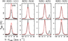 |
Fig. 1 Best fit to the SO lines towards the UCHII G75. On the x-axis, we show the velocity shift from the systemic velocity VLSR listed in Table 1. The red curves superimposed on the observed spectrum (in black) represent the best fit with one Gaussian component in the upper panels, and with two Gaussian components in the lower panels. |
3 Results
3.1 Line profiles
The best-fit results for all sources and all molecular species are reported in Appendix B. Tables B.1 and B.2 show the best-fit radial centroid velocities, and Tables B.3 and B.4 list the bestfit line widths at half maximum. Both parameters were obtained with MADCUBA, as described in Sect. 2.3.
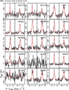
In most cases, the lines are very well fit with a single Gaussian. This is especially apparent in 13CS, C34S, SO+, NS, CCS, HCS+, CCCS, and NO. The transitions detected in this work have upper level energies up to ~40 K (Table 2), suggesting that they likely trace relatively cold material. Their spectral shapes confirm, this interpretation overall, even though in some sources clear high-velocity wings are present: the warm HMSC AFGLa, and the two HII regions G75 and NGC7 538. The transitions that are likely associated with shocked or warmer gas are those of SO, OCS, p-H2S, and SO2. Their upper-level energies are higher than 40 K, and they often show high-velocity wings. These wings are clearly present in the three sources already mentioned, and also towards the warm HMSC 05358a, the HMPOs 05358b, 18517, and 23385, and all UCHII regions except for 22134. The SO+, NS, and NO transitions do not show highvelocity wings, but their signal-to-noise ratios are much lower on average than those of the transitions discussed above, and the lack of these wings might therefore be due to the limited sensitivity.
Figures 2−4 show the comparison between the FWHM of the lines obtained with MADCUBA as explained in Sect. 2.3. From all possible combinations, we chose 13CS as the reference species because it is the best tracer of quiescent gas (Fig. 2). We also investigated correlations with HCS+ and CCS, which both have a temperature estimate. These comparisons allowed us to understand the species that are more likely associated with similar gas, and to search for significant variations among the different lines or species.
Figure 2 indicates that the FWHMs of the 13CS lines are positively correlated with those of almost all species, except for CCCS. The correlation is perfect with C34S (Pearson ρ correlation coefficient 0.99), good with HCS+, SO, NO, CCS, and SO+ (ρ ~ 0.81–0.92), and faint with H2CS, NS, H2S, OCS, and SO2 (ρ ~ 0.29–0.64). Clearly, the 13CS, C34S, and HCS+ observed transitions trace the same gas, based on their correlations and on the almost identical measured FWHM range. This is consistent with the fact that these species are all strictly chemically related to CS, and the observed transitions have the same quantum numbers (except for HCS+ J = 6–5). CCS is also tightly correlated with 13CS, and in all these species (C34S, 13CS, HCS+, and CCS), the FWHM never exceeds ~5 km s–1, indicating that they are all associated with relatively quiescent material.
Interestingly, the FWHMs derived from NS are narrower than those of 13CS, except in two UCHII regions, perhaps indicating that NS tends to trace the most quiescent and extended material in the less evolved stages. The positive correlation is very good with SO (ρ = 0.92) as well, but the SO lines have a systematically larger FWHM. This suggests that the SO emission is affected by a warmer, denser, and more turbulent component, for example associated with outflow cavities, which likely adds to the quiescent component. High-velocity non-Gaussian wings in SO are indeed found towards HMPOs and UCHIIs, while in cold HMSCs, only the quiescent component is detected. The FWHMs of the other O-bearing molecules, namely SO+, OCS, and SO2, are systematically larger than those of 13CS as well. This, and the additional evidence of hints of non-Gaussian wings in the spectra of OCS and SO2 (see Figs. A.14, A.15, A.17, A.18), indicate that these species trace more turbulent material. The nature of the SO+ emission is not easy to determine: its FWHMs are well correlated with those of 13CS, but, like SO, are systematically larger. Hence, they could contain both a quiescent and a turbulent component like SO. However, the lines do not show clear hints of non-Gaussian wings. The reason might be that the SO+ lines are fainter, and hence the lower signal-to-noise ratio in the spectra prevents us from detecting the high-velocity emission in the wings.
The molecule NO is found to be associated with both envelope material and outflow cavities in low-mass star-forming cores (Codella et al. 2018). Figure 2 (see also Table B.4) shows that the FWHMs of NO are smaller than those of SO, indicating that the emission from the envelope component is dominant in our NO lines. This is further supported by the lack of non-Gaussian wings in the spectra (see Fig. A.21), and it is consistent with the wider range in Eu of the SO lines with respect to the NO lines (19–100 K against 19 K, Tables 2 and 3).
Figures 3 and 4 show the comparison between the lines FWHM of HCS+ and CCS and those of the other tracers. The FWHMs of HCS+ correlate very well with those of C34S, SO, SO+, and NO (ρ ≥ 0.8). However, the relations closest to a y = x relation are found with C34S and NO, while SO and SO+ have larger FWHMs. Those of CCS (Fig. 4) only correlate well (ρ ≥ 0.8) with SO+ and C34S, but the range of values indicates that SO+ is associated with more turbulent material, as for HCS+. In summary, the lines of the C- and N-bearing species tend to trace the most quiescent, and probably extended, envelope of the sources. In particular, NS seems to be associated with the most quiescent gas in early sources, and then 13CS, C34S, HCS+, and CCS trace a similar, but maybe slightly farther inward, envelope. The O-bearing species are associated with more turbulent, and thus likely inner, regions of the cores based both on the larger FWHMs and on the non-Gaussian wings in evolved objects. Among these molecules, NO seems to trace the outermost layers, then SO and SO+ arise from slightly more turbulent inner regions, and finally, OCS and SO2 from the most turbulent inner regions. The origin of o-H2CS, p-H2S, and CCCS very strongly depends on the source, but while the o-H2CS and p-H2S lines show hints of non-Gaussian high-velocity wings in some targets (05358a, 05358b, 23385, 18517, G75, and NGC 7538), the CCCS lines are always Gaussian and hence are likely associated uniquely with an envelope component.
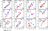 |
Fig. 2 Comparison between the lines FWHMs of the observed species and those of 13CS. In all plots, the black points indicate the cold HMSCs, the orange points the two warm HMSCs, the red points the HMPOs, and the blue points the UCHII regions. The dashed grey line indicates the locus y = x. The number in the upper left corner of each panel is the Pearson p correlation coefficient. |
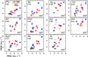 |
Fig. 3 Same as Fig. 2, but using HCS+ as reference species. The comparison with 13CS is shown in Fig. 2. |
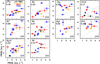 |
Fig. 4 Same as Fig. 2, but using CCS as reference species. The comparison with 13CS and HCS+ is shown in Figs. 2 and 3, respectively. |
3.2 Excitation temperatures and total column densities
The excitation temperatures, Tex, of the molecules listed in Tables 2 and 3 are shown in Table B.5. The total molecular column densities are listed in Tables B.6 and B.7. They were derived assuming LTE conditions, as described in Sect. 2.3. Tex were derived from MADCUBA as explained in Sect. 2.3 for the five species for which we detected at least two transitions with different energies, namely SO, CCS, HCS+, OCS, and SO2. For the species for which we have only one transition, that is, 13CS, C34S, p-H2S, o-H2CS, and CCCS, or multiple transitions with too similar energies of the levels (i.e. SO+, NS, and NO), we had to fix Tex to compute Ntot. The Tex we adopted is discussed below.
In Fig. 5, we investigate the correlations between each pair of measured excitation temperatures. As done for the FWHMs, we made a quantitative analysis by computing the Pearson ρ correlation coefficients. A clear positive correlation is found only between SO and SO2 (ρ = 0.78), even though the trend is strongly influenced by only one source. Fainter but still positive correlations are found between HCS+ and CCS, HCS+ and SO, and SO and CCS. Negative correlations are found between HCS+ and OCS, and CCS and OCS. The tracers associated with gas temperatures lower than ~30 K are HCS+ and CCS. The molecule SO also traces relatively cold gas because its Tex is between ~10–33 K, except for the UCHII region NGC 7538, for which Tex from SO is ~50 K. This source also causes the positive correlation between SO and SO2, which would be not significant without it (ρ ~ 0.14), and it is hence likely an outlier. The tracers that are clearly associated with material warmer than ~40 K are SO2 and OCS; both have temperatures higher than 45 K. All this is consistent with the previous suggestion based on the line FWHMs: The lines of the C-bearing species trace a colder extended envelope, SO traces maybe a denser and more compact but still relatively cold region, and OCS and SO2 trace the warmer and likely innermost regions.
The correlations between the FWHM of the lines shown in Figs. 2–4 allow us to determine the species that most likely arise from similar gas, and hence to assign the best-fit species to the molecules for which we do not have a direct Tex estimate. Figure 3 shows that 13CS, C34S, NS, and o-H2CS, have a good positive correlation with the FWHM of HCS+, and a similar velocity range. Hence, we fixed Tex from that of HCS+ to derive the column density of these species. Of the O-bearing species, the molecule NO shows the best positive correlation with HCS+ (ρ = 0.90). However, we also computed the correlation with SO and found a similar coefficient (ρ = 0.91). Therefore, because NO and SO are oxygen-containing species while HCS+ is not, we computed the NO column density fixing Tex to that of SO. The FWHM of SO+ also shows the best positive correlation with HCS+ (ρ = 0.8), but because of the fair correlation coefficient with SO (ρ = 0.65), the similar range of FWHMs measured, and their chemical relation, we adopted Tex from SO to compute the SO+ column density. The molecule p-H2S does not show a compelling correlation with any of the tracers we inspected. We thus decided to adopt Tex from SO because it is the most accurate estimate, owing to the large number of transitions with a relatively wide energy range (Eu = 19–56 K) on which it is based. For CCCS we lack a correlation with any tracer, and the dispersions are similar. We used Tex from HCS+ to be consistent with other C-only-bearing species.
For undetected species, an upper limit on Ntot was evaluated by ixing FWHM and Tex to those of the species that likely trace similar gas. For example, for OCS and SO2, we used FWHM and Tex from SO. By fixing FWHM and Tex in this way, we computed the upper limit on Ntot by simulating Gaussian lines below an intensity peak of ~3σ rms.
3.3 Molecular fractional abundances
From the molecular column densities in Tables B.6 and B.7, we computed the fractional abundances, X, by dividing them by the H2 total column densities, N(H2), given in Fontani et al. (2018). These are average values within an angular beam of 28″. Because the total column densities were estimated assuming that the emission is more extended than the beam, the abundances are average values within 28″. They are given in Tables 4 and 5.
We verified that the correlations, and tentative correlations, that were found based on the FWHMs with 13CS (Fig. 2) are also apparent in the fractional abundances. We performed the same check with the abundances of SO as reference species for the abundances of O-bearing molecules. The comparison with 13CS and SO are shown in Figs. 6 and 7, respectively. We first considered 13CS (Fig. 6). The clear correlations we found with C34S, SO, HCS+, and NO based on the FWHMs are confirmed between the abundances of these species and that of 13CS. For the other species, we find a positive correlation of X[13CS] with X[NS], X[SO+], X[p-H2S], X[SO2], X[OCS], and X[o-H2CS]. We stress, however, that these trends only consider the detected sources and do not include the upper limits. Hence, they must be taken with caution. Moreover, the strong correlations with OCS, p-H2S, and SO2 are mostly influenced by the UCHII G75. These correlations are weaker (ρ ≤ 0.5) without this target, while those with C34S, SO, HCS+, NO, and o-H2CS remain strong even when G75 is excluded from the statistical analysis. A very poor correlation (ρ ≤ 0.4) is found with CCS, and no correlation is found with CCCS, like in the FWHMs.
For the correlations with the SO fractional abundances (Fig. 7), we find positive correlations with 13CS, C34S, HCS+, NO, but also with o-H2CS, p-H2S, SO+, and OCS, which confirms the double origin of SO in both quiescent and turbulent material. SO is also positively correlated with NS and SO2, but the trend is determined mostly by one source alone, which is again the UCHII region G75, as for 13CS. No correlation between SO and CCS or CCCS is found. For 13CS, we stress that for some molecules the correlation coefficient is calculated without the upper limits (i.e. NS, SO+, p-H2S, OCS, SO2, and o-H2CS), and hence they should be considered with caution.
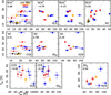 |
Fig. 5 Comparison between the excitation temperatures of the various molecules. In all plots, the black points indicate the cold HMSCs, the orange points the two warm HMSCs, the red points the HMPOs, and the blue points the UCHII regions. The dashed grey line indicates the locus y = x. |
4 Discussion
4.1 Chemistry of the tracers with correlated physical parameters
Based on the FWHMs, the Tex, and the molecular fractional abundances, we found correlations between some tracers. We discuss the possible chemical reasons of these correlations. We base our discussion on the chemical network of Shingledecker et al. (2020).
First, we note the perfect correlation in both FWHMs and abundances between 13CS and C34S, which shows a common origin for the two isotopologues, independent of either evolution and source physical properties. In particular, the correlation of the abundances also implies that fractionation effects of both carbon and sulphur are irrelevant. We discuss this point in more detail in Sect. 4.4. The relation between both CS isotopologues and HCS+ points to a ion-molecule schema for the formation of CS in which the dissociative recombination of HCS+ leads to CS. Formation of HCS+ may occur via both
 (1)
(1)
and
 (2)
(2)
where CS+ results from SO + C+, and/or CH + S+ reactions, and charge transfer between CS and H+. CS may also be formed through neutral-neutral reaction pathways from the reactions O + CCS and C + SO, which may stand for the FWHM correlations observed in Fig. 2 between 13CS and CCS, and 13CS and SO. The latter correlation is also observed between their abundances (Fig. 6). Moreover, because both CS isotopologues and SO have non-Gaussian high-velocity wings in the HMPO and UCHII stages (Figs. A.1, A.2, A.4, and A.5), they are likely both partially produced from grain sputtering in protostellar outflows in evolved sources.
The molecule NS is associated with the smallest FWHMs, except for the UCHII NGC 7538. NS is produced starting from atomic S either on grain surfaces or in the gas via
 (3)
(3)
 (4)
(4)
and it is mainly destroyed via
 (5)
(5)
Therefore, the fact that NS is associated with very quiescent gas could be due to the destruction of NS by atomic oxygen in evolved stages. Atomic oxygen could be more abundant in these stages owing to photodissociation of water (see e.g. van Dishoeck et al. 2021). If this is the case, a positive correlation between the abundances of NS and NO should be expected in evolved stages. In fact, we find a positive correlation between the two abundances (ρ ~ 0.65). We discuss this point in more detail in Sect. 4.2.
Abundances with respect to H2 of the analysed diatomic molecules.
Abundances with respect to H2 of the molecules with three and four atoms.
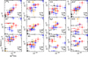 |
Fig. 6 Comparison between the fractional abundances of the observed species and that of 13CS. In all plots, the black points indicate the cold HMSCs, the orange points the two warm HMSCs, the red poins the HMPOs, and the blue points the UCHII regions. The empty triangles are upper limits. The number in the lower right corner of each panel is the Pearson p correlation coefficient. |
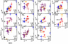 |
Fig. 7 Same as Fig. 6, but using SO as reference species. The comparison between SO and 13CS is shown in Fig. 6. |
4.2 Abundances as a function of the evolutionary stage
We have searched for relations between the fractional abundances and the source parameters that are thought to be evolutionary indicators, such as the kinetic gas temperature (Tk), the dust temperature (Tdust), the luminosity (L), and the luminosity-to-mass ratio (L/M). All parameters were derived from Herschel thermal dust emission measurements (Mininni et al. 2021), except for Tk which was derived from ammonia observations (Fontani et al. 2011).
The molecular fractional abundances as a function of the gas kinetic temperature are shown in Fig. 8. All except those of CCS and CCCS are positively correlated with Tk. For each molecule, we computed the Pearson p correlation coefficient and performed a linear regression fit to the data (plotted in logaritmic scale in Fig. 8). The strongest positive correlations are found for C34S, 13CS, HCS+, SO, SO2, and H2S, having all ρ ≥ 0.9, while the other tracers show a lower correlation. No significant correlation is found for CCS and CCCS. The plots of the abundances as a function of the other evolutionary indicators (Tdust, L, and M/L) are shown in Appendix C. We grouped the sulphur molecules into C-only-bearing (Fig. C.1), CH-bearing (Fig. C.2), O-only-bearing (Fig. C.3), and other species (Fig. C.4). The C-only-bearing species, namely C34S,13CS, CCS, and CCCS, and the CH-bearing species HCS+ and o-H2CS, do not show obvious trends overall with the four evolutionary parameters, except that with Tk. However, while C34S, 13CS, HCS+, and o-H2CS show hints of an increasing trend with Tdust, L, and M/L, especially for Tdust≥ 25 K and L ≥ 103 L⊙, CCS and CCCS do not show any trend over the full temperature (~ 10–100 K) and luminosity (~102–105 L⊙) ranges. Furthermore, CCCS is the only species detected in all the cold HMSCs, but not in the warm HMSCs (see Fig. A.19).
Both CCS and CCCS are thought to be gas-phase products mainly via
 (6)
(6)
 (7)
(7)
 (8)
(8)
 (9)
(9)
 (10)
(10)
 (11)
(11)
 (12)
(12)
and the dissociative recombination reactions (Eqs. (6), (7), and (10)) are the dominant formation pathways for both CCS and CCCS. The main destruction channel of CCS is via reactions with atomic oxygen and nitrogen that return CS, whereas CCCS does not react with atomic oxygen or nitrogen as a consequence of the presence of a (small) barrier, as discussed in Vidal et al. (2017). If this barrier is overtaken in warm(er) environments, CCCS starts to be destroyed. This would explain that the abundance in warm HMSCs is lower than in cold HMSCs. Then, the fact that CCCS is again present at later stages could be due to a renewed efficient production, even though the non-detection in two UCHIIs again demonstrates an efficient destruction in these later stages as well.
The abundances of the O-bearing species SO, SO+, and SO2 are positively correlated overall with Tdust, Tk, L, and M/L. The clearest trends are for SO and especially SO2, as both molecules show the best correlation with Tk (Fig. C.3). Finally, of the remaining species, which are are NS, OCS, and p-H2S (Fig. C.4), the latter shows a clearly increasing trend with all evolutionary parameters, in particular, with Tk, while NS and OCS show less obvious trends. Both SO2 and H2S are well-known shock tracers, and our study indicates that they are evolutionary indicators for high-mass star-forming regions.
We also computed the mean fractional abundances for each evolutionary stage. The results are shown in Fig. 9. In particular, for the HMSC group, the mean was computed separately for the cold sources (00117b, 20293a, and 22134b) and the warm sources (AFGLa and 05358a). In some tracers, the cold HMSCs were both undetected: SO+, NS, p-H2S, OCS, and SO2. For these, we computed the mean upper limit. The plot shows an increase in the mean abundances with the evolutionary stage in almost all molecules. However, the increase is different: (1) it jumps by about an order of magnitude from the cold HMSC group to the other groups for NS, p-H2S, and o-H2CS, and it then stays almost constant; (2) it gradually increases through all stages in SO, SO+, and SO2; (3) it increases by less than an order of magnitude from the cold HMSC group to the other groups for 13CS and HCS+, and it then stays almost constant; finally, (4) it is (almost) constant in all groups for NO, OCS, and CCS (but OCS contains several upper limits).
We start with the molecules that show marginal or no enhancement. The negligible increase for 13CS, NO, CCS, and HCS+ is consistent with the fact that they are associated with extended material that is likely not affected, or is only marginally affected, by inner protostellar activity. However, OCS is thought to be produced in protostellar shocks, but because we only have upper limits in the cold HMSC group, the negligible enhancement could simply be due to the fact that these upper limits are too high with respect to the real abundances. For the species that show significant enhancement, the clear increase observed for SO, SO+, SO2, p-H2S, and o-H2CS indicates a favoured production of these species in warm gas and/or protostellar outflows. In particular, the gradual increase up to the UCHII phase of SO, SO+, and SO2 could be due to the increasingly larger abundance of atomic oxygen with evolution, owing to photodissociation of water in the gas phase. The low water abundances of ~10−4 measured in protostellar environments (much lower than ~4×10⁻⁴ expected if all volatile oxygen is driven into water) were explained by strong UV radiation in shocks that dissociates water into O and OH (van Dishoeck et al. 2021; Tabone et al. 2021).
We summed the abundances of all S-bearing molecules to estimate the total budget of gaseous sulphur in each source. We call this sum Xtot[S] and show it in Fig. 10. The o-H2CS and p-H2S abundances were converted into the total abundances assuming their LTE relative ratio of 3/4 and 1/4, respectively.
The total abundance of CS was computed by multiplying the 13CS abundance for the average local ISM carbon isotope ratio of 68 (Milam et al. 2005). We also considered the upper limits in the sum, and hence, each source Xtot[S ] includes an upper limit to the total budget of gaseous sulphur, especially for the cold HMSCs, which are associated with the highest number of upper limits. Despite this, the minimum average value is found towards the cold HMSCs, and the maximum enhancement of sulphur is found towards the UCHIIs, which are the most evolved objects. The global increasing trend is likely due to the increasing amount of S that is sputtered from dust grains owing to the increasing protostellar activity with evolution. The largest Xtot [S] is ~10−7 found towards G75. Because the reference elemental abundance of atomic sulphur is 1.73×10⁻⁵ (Lodders 2003), this maximum enhancement is still lower by more than a factor 100 than the cosmic elemental abundance. This agrees with previous observational results and theoretical models (e.g. Esplugues et al. 2014; Fuente et al. 2016).
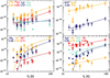 |
Fig. 8 Fractional abundances as a function of the kinetic temperature. Tk is derived from ammonia (Fontani et al. 2011). The four panels show sulphur-bearing molecules that contain only carbon (top left panel); carbon and hydrogen (top right panel); only oxygen (bottom left panel); and anything else (bottom right panel). The symbols without uncertainty are upper limits. The numbers below the label of each molecule are the Pearson ρ correlation coefficient. The curves represent linear fits to the data, including the upper limits plotted in logaritmic scale. |
4.3 Abundance ratios as a function of the evolutionary stage
Previous works suggested that some abundance ratios of the S-bearing species depend on the temperature of the host core. Herpin et al. (2009) studied two infrared- (IR) dark and two IR-bright high-mass dense cores in several sulphur-bearing molecules, and found that the SO/CS ratio increases from the IR-dark to the IR-bright objects owing to an increase in the SO abundance. On the other hand, el Akel et al. (2022) reported that the SO/CS ratio decreases from the cold envelope of intermediate-mass protostars to warmer inner regions. The SO/CS ratios we observed are shown in Fig. 11. The ratio is lowest in cold HMSCs, and it then slightly increases in the later stages, in agreement with the study of Herpin et al. (2009). Other ratios that were claimed to increase with the evolutionary stage by Herpin et al. (2009) are H2S/OCS and SO/SO2, while CS/H2S and OCS/SO2 are found to decrease. Figure 11 shows that the increasing trend for H2S/OCS and the decreasing trends for CS/H2S and OCS/SO2 are confirmed in our sources.
The SO/SO2 ratio was proposed by Wakelam et al. (2011) to decrease with time in massive cores. Our observations show a decrease by a factor 3–6 from the HMSCs to the later stages (Fig. 11). SO2 can be produced on the surfaces of dust grains via oxygenation of SO, but also in the gas phase via (e.g. Vastel et al. 2018)
 (13)
(13)
which is barrierless and favoured at high temperatures by the enhanced presence of OH in the gas, leading to a decrease in the SO/SO2 ratio.
Finally, the NO/NS ratio can be seen as a proxy to the O/S elemental abundance ratio. As discussed in Sect. 4.2, the atomic abundance of both S and O is expected to increase with the evolutionary stage because the enhancement of atomic S is due to dust grain evaporation and/or sputtering, and that of O to photodesorption and following photodissociation of water. We note that the NO/NS ratio is ~100 and constant in the evolved groups, while it is higher than 120 in the cold HMSCs. Figure 9 indicates that this is mostly due to the lower abundance of NS in the cold HMSCs because the abundance of NO is relatively constant in all evolutionary groups. This may be due to a higher depletion of S with respect to O in the early stages. Equation (5) indicates that NS is destroyed by atomic O to form NO. However, this channel is a very minor destruction mechanism of NO and has no impact on the NO/NS ratio.
Interestingly, the SO/13CS ratio below 13 in all evolutionary groups (see Fig. 11) indicates that the SO/12CS is smaller than 0.2 assuming the standard 12C/13C = 68 ratio, consistent with carbon-rich environments.
Furthermore, the NO/NS ratio is ~ 100 and constant in the evolved groups, and it is higher than 120 in cold HMSCs. This points to a higher depletion of S with respect to O in this early stage, and a similar relative abundance in the later stages. We stress, however, that care needs to be taken in interpreting these ratios because the emission of the various molecules can arise from different regions inside the telescope beam.
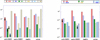 |
Fig. 9 Mean fractional abundances as a function of the evolutionary stage. The down-pointing arrows indicate mean upper limits. Left panel: measured mean abundances of S-bearing species containing oxygen and/or nitrogen. The sources are ordered from left to right according to their evolutionary stage (from HMSCs to UCHIIs). Right panel: same as the left panel for S-bearing species containing only carbon and/or hydrogen. |
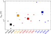 |
Fig. 10 Sum of the molecular fractional abundances in each source. The sources are indicated on the x-axis. The small symbols represent the total molecular abundances in each source, and the large symbols are the average values calculated in each group: cold HMSCs (in black), warm HMSCs (in orange), HMPOs (in red), and UCHIIs (in blue). |
4.4 Sulphur and carbon isotopic ratio
From 13CS and C34S J = 2−1, we estimated the double isotopic ratio 34S/32S×12C/13C. The reference Solar System values are 12C/13C~89, and 32S/34S~22 (Lodders 2003), so the reference solar value is 34S/32S×12C/13C~4. The local ISM 12C/13C ratio derived from molecular data is ~68 (Milam et al. 2005), and hence, in this case, 34S/32S×12C/13C would be ~3. The plot in Fig. 11 shows the average column density ratio C34S/13CS as a function of the evolutionary stage. The ratio is ~3, consistent with the local ISM 34S/32S×12C/13 value. In particular, it decreases from ~3 to ~2.3 from the cold HMSCs to the warm HMSCs, and then it is almost constant in the later stages.
Fractionation processes for sulphur are usually considered negligible in dense clouds, especially in warm cores, as indicated by theoretical and observational works (Loison et al. 2019; Humire et al. 2020; Yan et al. 2023). On the other hand, the models of Colzi et al. (2020) predict that the 12C/13C ratio in CS can reach values that are up to a factor ~3 higher with respect to the local value in cold (~10 K) and dense (2×104 cm−3) cores. These physical parameters are appropriate for the gaseous envelope of quiescent HMSCs, in which the measured C34S/13CS ratio is highest. The constant trend in warm, later stages indicates that local carbon (and sulphur) fractionation processes are irrelevant at these stages in the emission regions probed by our observations.
5 Summary and conclusions
We analysed observations of S-containing molecules obtained with the IRAM 30 m telescope towards 15 star-forming cores that we divided equally into the evolutionary stages HMSCs, HMPOs, and UCHIIs. The HMSCs were further divided into cold HMSCs and warm HMSCs, as was done in previous works. We derived column densities assuming LTE conditions of SO, SO+, NS, C34S, 13CS, S02, CCS, H2S, HCS+, OCS, H2CS, and CCCS. We also analysed for the first time the lines of the NO molecule to complement the analysis. For CCS, HCS+, SO, OCS, and SO2, we also derived the excitation temperatures. The line widths and excitation temperatures indicate that C34S, 13CS, CCS, HCS+, and NS trace preferentially quiescent and likely extended material, SO and maybe SO+ both quiescent and turbulent material depending on the target, while OCS, and SO2 trace warmer, more turbulent, and likely denser and more compact material. The nature of the emission of the H2S, H2CS, and CCCS emission is less clear. We also found a globally increasing trend of the total gaseous sulphur from cold HMSCs to UCHIIs. This is likely due to the increasing amount of S that is sputtered from dust grains owing to the increasing protostellar activity with evolution. Still, the maximum total abundance that we find is ~10−7 towards the UCHII G75, which is two orders of magnitude lower than the elemental S abundance. The abundances that show the best positive correlations with the evolutionary indicators are those of SO and SO2, and in general, oxygen-bearing species have higher abundances in more evolved stages than carbon-bearing species, perhaps due to the larger availability of atomic oxygen with evolution produced by photodissociation of water. We confirm that the abundance ratios SO/CS, H2S/OCS, CS/H2S, and OCS/SO2, which were claimed to be possible evolutionary indicators, are found to vary with the evolution in our study as well. Interestingly, we find that the NO/NS ratio, which can be considered a proxy of the O/S abundance ratio, is higher in the HMSCs than in the other three groups, perhaps due to the higher S-depletion with respect to O in this early stage. Our observational work represents an observational test-bed for theoretical studies aimed at modelling the chemistry of sulphur during the evolution of high-mass star-forming cores, and it needs to be complemented by observations with higher angular resolution to overcome possible problems due to different filling factors.
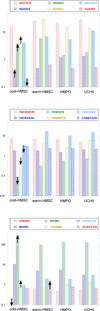 |
Fig. 11 Column density ratios as a function of the evolutionary stage. The upward-pointing arrows show the lower limits. The downward-pointing show the upper limits. |
Acknowledgements
We thank the anonymous Referee for their careful reading of the paper and their constructive comments. F.F. is grateful to the IRAM staff for their precious help during observations. L.C. acknowledges financial support through the Spanish grant PID2019-105552RB-C41 funded by MCIN/AEI/10.13039/501100011033. This work is based on observations carried out under project number 116-16 with the IRAM 30 m telescope. IRAM is supported by INSU/CNRS (France), MPG (Germany) and IGN (Spain).
Appendix A Spectra
In this appendix, we show the spectra of all molecular species we analysed. For those with more than three detected transitions, we show only the brightest spectra.
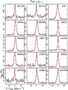 |
Fig. A.1 Spectra of the 13CS J = 2 − 1 lines. On the x-axis, we show the velocity shift from the systemic velocity VLSR listed in Table 1. In each frame, the red curve represents the best Gaussian fit performed with MADCUBA (see Sect. 2.3). The first column contains the HMSCs, the second the HMPOs, and the third the UCHIIs. |
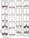 |
Fig. A.3 Spectra of SO J(K) = 2(1) − 1(1), 6(5) − 5(4), 5(6) − 4(5), and 6(6) − 5(5) observed towards the HMSCs. The red curves indicate the best-fit Gaussians performed with MADCUBA. |
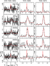 |
Fig. A.8 Spectra of CCS N(J) = 7(6) − 6(5), 7(7) − 6(6), and 7(8) − 6(7) for the HMSCs. The red curves indicate the best-fit Gaussian curves obtained with MADCUBA |
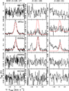 |
Fig. A.13 Spectra obtained towards the HMSCs of the OCS J = 18 − 17, J = 21 − 20 and J = 22 − 21 lines. The red curves indicate the best fit obtained with MADCUBA. |
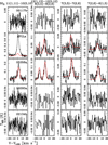 |
Fig. A.16 Spectra obtained towards the HMSCs of the SO2 J(Ka, Kb) = 11(1,11) − 10(0,10), 13(1,13) − 12(0,12), 8(3,5) − 8(2, 6), 7(3,5) − 7(2, 6), and 7(2, 6) − 6(1,5) lines. The red curves indicate the best fit obtained with MADCUBA. |
Appendix B Best-fit parameters
In this appendix, we include the best-fit parameters of the species we analysed that were obtained with MADCUBA (Sect. 2.3): centroid velocities, line widths at half maximum, excitation temperatures, and total column densities.
Best-fit centroid velocities in km s−1 for the molecules with two atoms. The numbers in brackets give the uncertainties.
Excitation temperatures (in K) derived with MADCUBA.
Column densities in cm−2 of the analysed diatomic molecules
Appendix C Plots of fractional abundances versus all evolutionary parameters
In this appendix, we show plots of the fractional abundances of all molecular species we analysed as a function of the physical parameters expected to vary with evolution: dust temperature (Tdust), kinetic temperature (Tk, already shown in Fig. 8), source bolometric luminosity (L), and lumonisity-to-mass ratio (M/L).
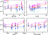 |
Fig. C.1 Fractional abundances as a function of evolutionary parameters. Top left panel: Measured abundances of molecules containing only sulphur and carbon as a function of the dust temperature. Td was derived by fitting the SED (Mininni et al. 2021). The symbols without uncertainty are upper limits. The curves represent linear fits to the data, including upper limits. Top right panel: Same abundances as in the top left panel as a function of the kinetic gas temperature derived from ammonia (Fontani et al. 2011); Bottom left panel: Same abundances as a function of the bolometric source luminosity derived from the SED (Mininni et al. 2021); Bottom right panel: Same abundances as a function of the luminosity-to-mass ratio (Mininni et al. 2021). |
References
- Adams, F. C. 2010, ARA & A, 48, 47 [NASA ADS] [CrossRef] [Google Scholar]
- Altwegg, K., Balsiger, H., & Fuselier, S. A. 2019, ARA & A, 57, 113 [NASA ADS] [CrossRef] [Google Scholar]
- Anderson, D. E., Bergin, E. A., Maret, S., & Wakelam, V. 2013, Apl, 779, 141 [Google Scholar]
- Asplund, M., Grevesse, N., Sauvai, A. I., & Scott, P. 2009, ARA & A, 47, 481 [NASA ADS] [CrossRef] [Google Scholar]
- Beuther, H., Zhang, Q., Bergin, E. A., & Sridharan, T. K. 2009, AI, 137, 406 [NASA ADS] [Google Scholar]
- Boogert, A. C. A., Gerakines, P. A., & Whittet, D. C. B. 2015, ARA & A, 53, 541 [NASA ADS] [CrossRef] [Google Scholar]
- Calmonte, U., Altwegg, K., Balsiger, H., et al. 2016, MNRAS, 462, 253 [Google Scholar]
- Carpenter, I. M. 2000, AI, 120, 3139 [NASA ADS] [Google Scholar]
- Cazaux, S., Carrascosa, H., Muñoz Caro, G. M., et al. 2022, A & A, 657, A100 [NASA ADS] [CrossRef] [EDP Sciences] [Google Scholar]
- Cernicharo, I., Cabezas, C., & Agúndez, M. 2021, A & A, 648, A3 [CrossRef] [EDP Sciences] [Google Scholar]
- Codella, C., Viti, S., Lefloch, B., et al. 2018, MNRAS, 474, 5694 [NASA ADS] [CrossRef] [Google Scholar]
- Coletta, A., Fontani, F., Rivilla, V. M., et al. 2020, A & A, 641, A54 [CrossRef] [EDP Sciences] [Google Scholar]
- Colzi, L., Fontani, F., Caselli, P., et al. 2018, A & A, 609, A129 [NASA ADS] [CrossRef] [EDP Sciences] [Google Scholar]
- Colzi, L., Fontani, F., Caselli, P., et al. 2019, MNRAS, 485, 5543 [NASA ADS] [CrossRef] [Google Scholar]
- Colzi, L., Sipilä, O., Roueff, E., Caselli, P., & Fontani, F. 2020, A & A, 640, A51 [NASA ADS] [CrossRef] [EDP Sciences] [Google Scholar]
- Drdla, K., Knapp, G. R., & van Dishoeck, E. F. 1989, Apl, 345, 815 [Google Scholar]
- el Akel, M., Kristensen, L. E., Le Gal, R., et al. 2023, A & A, 659, A100 [Google Scholar]
- Endres, P., Schlemmer, S., Schilke, P., Stutzki, I., & Müller, H. S. P. 2016, I. Mol. Spectrosc, 327, 95 [NASA ADS] [CrossRef] [Google Scholar]
- Esplugues, G. B., Viti, S., Goicoechea, I. R., & Cernicharo, I. 2014, A & A, 567, A95 [NASA ADS] [CrossRef] [EDP Sciences] [Google Scholar]
- Esplugues, G., Fuente, A., Navarro-Almaida, D., et al. 2022, A & A, 662, A52 [NASA ADS] [CrossRef] [EDP Sciences] [Google Scholar]
- Esteban, C., Peimbert, M., García-Rojas, I., et al. 2004, MNRAS, 355, 229 [NASA ADS] [CrossRef] [Google Scholar]
- Evans, N. I.II, Dunham, M .M., Iørgensen, I. K., et al. 2009, ApIS, 181, 321 [Google Scholar]
- Fontani, F., Cesaroni, R., Testi, L., et al. 2004, A & A, 414, 299 [NASA ADS] [CrossRef] [EDP Sciences] [Google Scholar]
- Fontani, F., Pascucci, L., Caselli, P., et al. 2007, A & A, 470, 639 [NASA ADS] [CrossRef] [EDP Sciences] [Google Scholar]
- Fontani, F., Palau, Aina, Caselli, P., et al. 2011, A & A, 529, A7 [Google Scholar]
- Fontani, F., Sakai, T., Furuya, K., et al. 2014, MNRAS, 440, 448 [NASA ADS] [CrossRef] [Google Scholar]
- Fontani, F., Caselli, P., Palau, A., Bizzocchi, L., & Ceccarelli, C. 2015a, Apl, 808, L46 [Google Scholar]
- Fontani, F., Busquet, G., Palau, A., et al. 2015b, A & A, 575, A87 [NASA ADS] [CrossRef] [EDP Sciences] [Google Scholar]
- Fontani, F., Vagnoli, A., Padovani, M., et al. 2018, MNRAS, 481, L79 [NASA ADS] [CrossRef] [Google Scholar]
- Fontani, E., Colzi, L., Redaelli, E., Sipilä, O., & Caselli, P. 2021, A & A, 651, A94 [NASA ADS] [CrossRef] [EDP Sciences] [Google Scholar]
- Fuente, A., Cernicharo, I., Roueff, E., et al. 2016, A & A, 593, A94 [NASA ADS] [CrossRef] [EDP Sciences] [Google Scholar]
- Fuente, A., Navarro, D. G., Caselli, P., et al. 2019, A & A, 624, A105 [NASA ADS] [CrossRef] [EDP Sciences] [Google Scholar]
- Fuente, A., Rivière-Marichalar, P., Beitia-Antero, L., et al. 2023, A & A, 670, A114 [NASA ADS] [CrossRef] [EDP Sciences] [Google Scholar]
- Goicoechea, I. R., Pety, I., Gerin, M., et al. 2006, A & A, 456, 565 [NASA ADS] [CrossRef] [EDP Sciences] [Google Scholar]
- Hatchell, I., Thompson, M.A., Mllar, T. I., & MacDonald, G. H. 1998, A & A, 338, 713 [NASA ADS] [Google Scholar]
- Herpin, F., Marseille, M., Wakelam, V., Bontemps, S., & Lis, D. C. 2009, A & A, 504, 853 [NASA ADS] [CrossRef] [EDP Sciences] [Google Scholar]
- Heyl, J., Sellentin, E., Holdship, J., & Viti, S. 2022, MNRAS, 517, 38 [CrossRef] [Google Scholar]
- Hily-Blant, P., Pineau des Forêts, G., Faure, A., & Lique, F. 2022, A & A, 658, A168 [NASA ADS] [CrossRef] [EDP Sciences] [Google Scholar]
- Holdship, J., Jiménez-Serra, I., Viti, S., et al. 2019, ApJ, 878, 64 [NASA ADS] [CrossRef] [Google Scholar]
- Howk, J. C., Sembach, K. R., & Savage, B. D. 2006, ApJ, 637, 333 [NASA ADS] [CrossRef] [Google Scholar]
- Humire, P. K., Thiel, V., Henkel, C., et al. 2020, A & A, 642, A222 [NASA ADS] [CrossRef] [EDP Sciences] [Google Scholar]
- Jenkins, E. B. 2009, ApJ, 700, 1299 [Google Scholar]
- Jiménez-Escobar, A., & Munoz Caro, G. M. 2011, A & A, 536, A91 [CrossRef] [EDP Sciences] [Google Scholar]
- Kurtz, S., Cesaroni, R., Churchwell, E., Hofner, P., & Walmsley, C. M. 2000, in Protostars and Planets IV, eds. V., Mannings, A. P., Boss, & S. S. Russell (Tucson: University of Arizona Press), 299 [Google Scholar]
- Kutner, M. L., & Ulich, B. L. 1981, ApJ, 250, 341 [NASA ADS] [CrossRef] [Google Scholar]
- Laas, J., & Caselli, P. 2019, A & A, 624, A118 [Google Scholar]
- Lodders, K. 2003, ApJ, 591, 1220 [Google Scholar]
- Loison, J.-C., Wakelam, V., Gratier, P., et al. 2019, MNRAS, 485, 5777 [Google Scholar]
- Martin, S., Martín-Pintado, J., Blanco-Sánchez, C., et al. 2019, A & A, 631, A159 [CrossRef] [EDP Sciences] [Google Scholar]
- McClure, M. K., Rocha, W. R. M., Pontoppidan, K. M., et al. 2023, Nat. Astron., 7, 431 [NASA ADS] [CrossRef] [Google Scholar]
- McGuire, B. A. 2018, ApJS, 239, 17 [Google Scholar]
- Milam, S. N., Savage, C., Brewster, M. A., & Ziurys, L. M. 2005, ApJ, 634, 1126 [NASA ADS] [CrossRef] [Google Scholar]
- Millar, T. J., Adams, N. G., Smith, D., Lindinger, W., & Villinger, H. 1986, MNRAS, 221, 673 [NASA ADS] [CrossRef] [Google Scholar]
- Mininni, C., Fontani, F., Rivilla, V. M., et al. 2018, MNRAS, 476, A39 [Google Scholar]
- Mininni, C., Fontani, F., Sánchez-Monge, A., Rivilla, V. M., & Beltrán, M. T. 2021, A & A, 653, A87 [NASA ADS] [CrossRef] [EDP Sciences] [Google Scholar]
- Navarro-Almaida, D., Le Gal, R., Fuente, A., et al. 2020, A & A, 637, A39 [NASA ADS] [CrossRef] [EDP Sciences] [Google Scholar]
- Oppenheimer, M., & Dalgarno, A. 1974, ApJ, 187, 231 [NASA ADS] [CrossRef] [Google Scholar]
- Pickett, H. M., Poynter, R. L., Cohen, E. A., et al. 1998, JQSRT, 60, 883 [NASA ADS] [CrossRef] [Google Scholar]
- Pineau des Forêts, G., Roueff, E., & Flower, D. R. 1986, MNRAS, 223, 743 [CrossRef] [Google Scholar]
- Pfalzner, S. 2013, A & A, 549, A82 [NASA ADS] [CrossRef] [EDP Sciences] [Google Scholar]
- Rivilla, V. M., Beltrán, M. T., Cesaroni, R., et al. 2017, A & A, 598, A59 [NASA ADS] [CrossRef] [EDP Sciences] [Google Scholar]
- Rivilla, V. M., Colzi, L., Fontani, et al. 2020a, MNRAS, 496, 1990 [NASA ADS] [CrossRef] [Google Scholar]
- Rivilla, V. M., Drozdovskaya, M. N., Altwegg, K., et al. 2020b, MNRAS, 492, 1180 [NASA ADS] [CrossRef] [Google Scholar]
- Shingledecker, C. N., Lamberts, T., Laas, J. C., et al. 2020, ApJ, 888, 52 [Google Scholar]
- Tabone, B., van Hemert, M .C., van Dishoeck, E. F., & Black, J. H. 2021, A & A, 650, A192 [NASA ADS] [CrossRef] [EDP Sciences] [Google Scholar]
- Taniguchi, K., Saito, M., Sridharan, T. K., & Minamidani, T. 2018, ApJ, 854, 133 [NASA ADS] [CrossRef] [Google Scholar]
- Turner, B. 1995, ApJ, 455, 556 [NASA ADS] [CrossRef] [Google Scholar]
- van Dishoeck, E. F., Kristensen, L. E., Mottram, J. C., et al. 2021, A & A, 648, A24 [CrossRef] [EDP Sciences] [Google Scholar]
- Vastel, C., Quénard, D., Le Gal, R., et al. 2018, MNRAS, 478, 5514 [Google Scholar]
- Vasyunina, T., Linz, H., Henning, Th., et al. 2011, A & A, 527, A88 [NASA ADS] [CrossRef] [EDP Sciences] [Google Scholar]
- Vidal, T. H. G., Loison, J.-C., Jaziri, A. Y., et al. 2017, MNRAS, 469, 435 [Google Scholar]
- Wakelam, V., Hersant, F., & Herpin, F. 2011, A & A, 529, A112 [NASA ADS] [CrossRef] [EDP Sciences] [Google Scholar]
- Wang, Y., Audard, M., Fontani, F., et al. 2016, A & A, 587, A69 [NASA ADS] [CrossRef] [EDP Sciences] [Google Scholar]
- Woods, P. M., Occhiogrosso, A., Viti, S., et al. 2015, MNRAS, 450, 1256 [Google Scholar]
- Yan, Y. T., Henkel, C., Kobayashi, C., et al. 2023, A & A, 670, A98 [NASA ADS] [CrossRef] [EDP Sciences] [Google Scholar]
- Zanchet, A., Agúndez, M., Herrero, V. J., et al. 2013, AJ, 146, 125 [NASA ADS] [CrossRef] [Google Scholar]
MADCUBA is a software developed in the Madrid Center of Astro-biology (INTA-CSIC), which enables visualising and analysing single spectra and data cubes: https://cab.inta-csic.es/madcuba/.
All Tables
Best-fit centroid velocities in km s−1 for the molecules with two atoms. The numbers in brackets give the uncertainties.
All Figures
|
Fig. 1 Best fit to the SO lines towards the UCHII G75. On the x-axis, we show the velocity shift from the systemic velocity VLSR listed in Table 1. The red curves superimposed on the observed spectrum (in black) represent the best fit with one Gaussian component in the upper panels, and with two Gaussian components in the lower panels. |
| In the text | |
|
Fig. 2 Comparison between the lines FWHMs of the observed species and those of 13CS. In all plots, the black points indicate the cold HMSCs, the orange points the two warm HMSCs, the red points the HMPOs, and the blue points the UCHII regions. The dashed grey line indicates the locus y = x. The number in the upper left corner of each panel is the Pearson p correlation coefficient. |
| In the text | |
|
Fig. 3 Same as Fig. 2, but using HCS+ as reference species. The comparison with 13CS is shown in Fig. 2. |
| In the text | |
|
Fig. 4 Same as Fig. 2, but using CCS as reference species. The comparison with 13CS and HCS+ is shown in Figs. 2 and 3, respectively. |
| In the text | |
|
Fig. 5 Comparison between the excitation temperatures of the various molecules. In all plots, the black points indicate the cold HMSCs, the orange points the two warm HMSCs, the red points the HMPOs, and the blue points the UCHII regions. The dashed grey line indicates the locus y = x. |
| In the text | |
|
Fig. 6 Comparison between the fractional abundances of the observed species and that of 13CS. In all plots, the black points indicate the cold HMSCs, the orange points the two warm HMSCs, the red poins the HMPOs, and the blue points the UCHII regions. The empty triangles are upper limits. The number in the lower right corner of each panel is the Pearson p correlation coefficient. |
| In the text | |
|
Fig. 7 Same as Fig. 6, but using SO as reference species. The comparison between SO and 13CS is shown in Fig. 6. |
| In the text | |
|
Fig. 8 Fractional abundances as a function of the kinetic temperature. Tk is derived from ammonia (Fontani et al. 2011). The four panels show sulphur-bearing molecules that contain only carbon (top left panel); carbon and hydrogen (top right panel); only oxygen (bottom left panel); and anything else (bottom right panel). The symbols without uncertainty are upper limits. The numbers below the label of each molecule are the Pearson ρ correlation coefficient. The curves represent linear fits to the data, including the upper limits plotted in logaritmic scale. |
| In the text | |
|
Fig. 9 Mean fractional abundances as a function of the evolutionary stage. The down-pointing arrows indicate mean upper limits. Left panel: measured mean abundances of S-bearing species containing oxygen and/or nitrogen. The sources are ordered from left to right according to their evolutionary stage (from HMSCs to UCHIIs). Right panel: same as the left panel for S-bearing species containing only carbon and/or hydrogen. |
| In the text | |
|
Fig. 10 Sum of the molecular fractional abundances in each source. The sources are indicated on the x-axis. The small symbols represent the total molecular abundances in each source, and the large symbols are the average values calculated in each group: cold HMSCs (in black), warm HMSCs (in orange), HMPOs (in red), and UCHIIs (in blue). |
| In the text | |
|
Fig. 11 Column density ratios as a function of the evolutionary stage. The upward-pointing arrows show the lower limits. The downward-pointing show the upper limits. |
| In the text | |
|
Fig. A.1 Spectra of the 13CS J = 2 − 1 lines. On the x-axis, we show the velocity shift from the systemic velocity VLSR listed in Table 1. In each frame, the red curve represents the best Gaussian fit performed with MADCUBA (see Sect. 2.3). The first column contains the HMSCs, the second the HMPOs, and the third the UCHIIs. |
| In the text | |
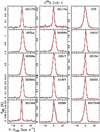 |
Fig. A.2 Same as Fig. A.1 for the C34S J = 2 − 1 lines. |
| In the text | |
|
Fig. A.3 Spectra of SO J(K) = 2(1) − 1(1), 6(5) − 5(4), 5(6) − 4(5), and 6(6) − 5(5) observed towards the HMSCs. The red curves indicate the best-fit Gaussians performed with MADCUBA. |
| In the text | |
 |
Fig. A.4 Same as Fig. A.3 for the HMPOs. |
| In the text | |
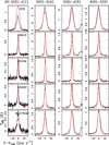 |
Fig. A.5 Same as Fig. A.3 for the UCHIIs. |
| In the text | |
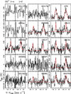 |
Fig. A.6 Same as Fig. A.1 for the SO+ J = 11/2 − 9/2 lines. |
| In the text | |
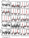 |
Fig. A.7 Same as Fig. A.1 for the NS J = 11/2 − 9/2, F = 13/2 − 11/2 lines. |
| In the text | |
|
Fig. A.8 Spectra of CCS N(J) = 7(6) − 6(5), 7(7) − 6(6), and 7(8) − 6(7) for the HMSCs. The red curves indicate the best-fit Gaussian curves obtained with MADCUBA |
| In the text | |
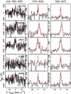 |
Fig. A.9 Same as Fig. A.8 for the HMPOs lines. |
| In the text | |
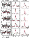 |
Fig. A.10 Same as Fig. A.8 the UCHIIs. |
| In the text | |
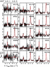 |
Fig. A.11 Same as Fig. A.1 for the HCS+ J = 2 − 1 and J = 6 − 5 lines. |
| In the text | |
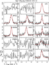 |
Fig. A.12 Same as Fig. A.1 for the H2S J(Ka, Kb = 2(2,0) − 2(1,1) lines. |
| In the text | |
|
Fig. A.13 Spectra obtained towards the HMSCs of the OCS J = 18 − 17, J = 21 − 20 and J = 22 − 21 lines. The red curves indicate the best fit obtained with MADCUBA. |
| In the text | |
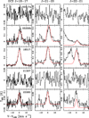 |
Fig. A.14 Same as Fig. A.13 for the HMPOs. |
| In the text | |
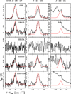 |
Fig. A.15 Same as Fig. A.13 for the UCHIIs. |
| In the text | |
|
Fig. A.16 Spectra obtained towards the HMSCs of the SO2 J(Ka, Kb) = 11(1,11) − 10(0,10), 13(1,13) − 12(0,12), 8(3,5) − 8(2, 6), 7(3,5) − 7(2, 6), and 7(2, 6) − 6(1,5) lines. The red curves indicate the best fit obtained with MADCUBA. |
| In the text | |
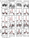 |
Fig. A.17 Same as Fig. A.16 for HMPOs. |
| In the text | |
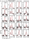 |
Fig. A.18 Same as Fig. A.16 for UCHIIs. |
| In the text | |
 |
Fig. A.19 Same as Fig. A.1 for the CCCS J = 15 − 14 lines. |
| In the text | |
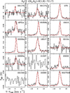 |
Fig. A.20 Same as Fig. A.1 for the H2CS J(Ka), Kb = 8(1,8) − 7(1,7) lines. |
| In the text | |
|
Fig. C.1 Fractional abundances as a function of evolutionary parameters. Top left panel: Measured abundances of molecules containing only sulphur and carbon as a function of the dust temperature. Td was derived by fitting the SED (Mininni et al. 2021). The symbols without uncertainty are upper limits. The curves represent linear fits to the data, including upper limits. Top right panel: Same abundances as in the top left panel as a function of the kinetic gas temperature derived from ammonia (Fontani et al. 2011); Bottom left panel: Same abundances as a function of the bolometric source luminosity derived from the SED (Mininni et al. 2021); Bottom right panel: Same abundances as a function of the luminosity-to-mass ratio (Mininni et al. 2021). |
| In the text | |
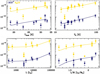 |
Fig. C.2 Same as Fig. C.1 for molecules containing only sulphur, carbon, and hydrogen. |
| In the text | |
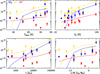 |
Fig. C.3 Same as Fig. C.1 for molecules containing only sulphur and oxygen. |
| In the text | |
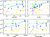 |
Fig. C.4 Same as Fig. C.1 for all other molecules. |
| In the text | |
Current usage metrics show cumulative count of Article Views (full-text article views including HTML views, PDF and ePub downloads, according to the available data) and Abstracts Views on Vision4Press platform.
Data correspond to usage on the plateform after 2015. The current usage metrics is available 48-96 hours after online publication and is updated daily on week days.
Initial download of the metrics may take a while.