| Issue |
A&A
Volume 678, October 2023
|
|
|---|---|---|
| Article Number | A166 | |
| Number of page(s) | 14 | |
| Section | The Sun and the Heliosphere | |
| DOI | https://doi.org/10.1051/0004-6361/202347011 | |
| Published online | 18 October 2023 | |
Three-dimensional relation between coronal dimming, filament eruption, and CME
A case study of the 28 October 2021 X1.0 event⋆
1
Skolkovo Institute of Science and Technology, Bolshoy Boulevard 30, Bld. 1, 121205 Moscow, Russia
e-mail: This email address is being protected from spambots. You need JavaScript enabled to view it.
2
NorthWest Research Associates, 3380 Mitchell Lane, Boulder, 80301 CO, USA
3
University of Graz, Institute of Physics, Universitätsplatz 5, 8010 Graz, Austria
4
University of Graz, Kanzelhöhe Observatory for Solar and Environmental Research, Kanzelhöhe 19, 9521 Treffen, Austria
5
Hvar Observatory, Faculty of Geodesy, University of Zagreb, Kaciceva 26, 10000 Zagreb, Croatia
Received:
25
May
2023
Accepted:
16
August
2023
Abstract
Context. Coronal dimmings are localized regions of reduced emission in the extreme-ultraviolet (EUV) and soft X-rays formed as a result of the expansion and mass loss by coronal mass ejections (CMEs) low in the corona. Distinct relations have been established between coronal dimmings (intensity, area, magnetic flux) and key characteristics of the associated CMEs (mass and speed) by combining coronal and coronagraphic observations from different viewpoints in the heliosphere.
Aims. We investigate the relation between the spatiotemporal evolution of the dimming region and both the dominant direction of the filament eruption and CME propagation for the 28 October 2021 X1.0 flare/CME event observed from multiple viewpoints in the heliosphere by Solar Orbiter, STEREO-A, SDO, and SOHO.
Methods. We present a method for estimating the dominant direction of the dimming development based on the evolution of the dimming area, taking into account the importance of correcting the dimming area estimation by calculating the surface area of a sphere for each pixel. To determine the propagation direction of the flux rope during early CME evolution, we performed 3D reconstructions of the white-light CME by graduated cylindrical shell modeling (GCS) and 3D tie-pointing of the eruptive filament.
Results. The dimming evolution starts with a radial expansion and later propagates more to the southeast. The orthogonal projections of the reconstructed height evolution of the prominent leg of the erupting filament onto the solar surface are located in the sector of the dominant dimming growth, while the orthogonal projections of the inner part of the GCS reconstruction align with the total dimming area. The filament reaches a maximum speed of ≈250 km s−1 at a height of about ≈180 Mm before it can no longer be reliably followed in the EUV images. Its direction of motion is strongly inclined from the radial direction (64° to the east, 32° to the south). The 3D direction of the CME and the motion of the filament leg differ by 50°. This angle roughly aligns with the CME half-width obtained from the CME reconstruction, suggesting a relation between the reconstructed filament and the associated leg of the CME body.
Conclusions. The dominant propagation of the dimming growth reflects the direction of the erupting magnetic structure (filament) low in the solar atmosphere, though the filament evolution is not directly related to the direction of the global CME expansion. At the same time, the overall dimming morphology closely resembles the inner part of the CME reconstruction, validating the use of dimming observations to obtain insight into the CME direction.
Key words: Sun: coronal mass ejections (CMEs) / Sun: filaments / prominences / Sun: corona / Sun: flares / methods: data analysis
Movies associated to Figs. 3 and 7 are available at https://www.aanda.org.
© The Authors 2023
 Open Access article, published by EDP Sciences, under the terms of the Creative Commons Attribution License (https://creativecommons.org/licenses/by/4.0), which permits unrestricted use, distribution, and reproduction in any medium, provided the original work is properly cited.
This article is published in open access under the Subscribe to Open model. This email address is being protected from spambots. You need JavaScript enabled to view it. to support open access publication.
1. Introduction
Coronal mass ejections (CMEs) are large-scale eruptions in the solar corona and are associated with huge energy release (Harrison 1995). These phenomena are very large quantities of the magnetized plasma with masses up to 1013 kg that are ejected from the Sun into interplanetary space with speeds in the range of ≈100−3000 km s−1 (Gopalswamy et al. 2009; Webb & Howard 2012). Earth-directed events can lead to a multitude of space weather effects in geospace, including power network knockouts, disturbances of the radio signal, and various anomalies in the functionality of satellites (e.g., reviews by Pulkkinen 2007; Koskinen et al. 2017; Temmer 2021). However, measurements of CME parameters, especially for Earth-directed events observed as halo-type events for spacecraft located along the Sun–Earth line, may be strongly affected by the projection effects (Burkepile et al. 2004; Gopalswamy et al. 2000). Moreover, the instruments traditionally used to analyze them, such as coronagraphs, occult the early part of the CME evolution in the low corona. The analysis of CME manifestations in the low corona, including filament eruptions and coronal dimmings, is therefore important for our understanding of the initiation mechanism and the early evolution of CMEs.
Coronal dimmings are regions of strongly reduced emission in extreme-ultraviolet (EUV; Thompson et al. 1998; Zarro et al. 1999) and soft X-ray (Hudson et al. 1996; Sterling & Hudson 1997) wavelengths occurring in association with CMEs. They are direct signatures of the expansion and ejection of coronal plasma by the CME (Thompson et al. 1998; Harrison & Lyons 2000). The mass-loss nature of their appearance is supported by the presence of plasma outflows detected in spectroscopic observations in the EUV (e.g., Harrison & Lyons 2000; Harra & Sterling 2001; Tian et al. 2012; Veronig et al. 2019) and the intensity decrease observed at multiple wavelengths (Zarro et al. 1999; Chertok & Grechnev 2003). Moreover, differential emission measure (DEM) diagnostics reveal impulsive drops in coronal dimming regions by up to 70% of the pre-event values (López et al. 2017; Vanninathan et al. 2018; Veronig et al. 2019). Recent statistical studies of coronal dimming events observed on-disk (Mason et al. 2016; Aschwanden 2016; Krista & Reinard 2017; Dissauer et al. 2019) by Solar Dynamics Observatory (SDO; Pesnell et al. 2012) and off-limb (Chikunova et al. 2020) by Solar TErrestrial Relations Observatory (STEREO; Kaiser et al. 2008) satellites reveal distinct correlations between characteristic dimming parameters and the speed and mass of the associated CMEs.
During the history of their observations, coronal dimmings were widely acknowledged as reliable indicators of front-side CMEs (Thompson et al. 2000), as they appear on the visible part of the solar disk. More detailed monitoring (Mandrini et al. 2007; Wills-Davey & Attrill 2009; Temmer et al. 2011; Dissauer et al. 2018a) and magnetohydrodynamical (MHD) simulations (Downs et al. 2012; Prasad et al. 2020) show that the locations of the so-called “core” dimmings map the footpoints of the erupting flux rope, while the spatial growth of the more wide-spread secondary dimmings indicates the expansion of the overlying magnetic structures of the CME expansion in the low corona. Together with other CME manifestations in the corona, dimmings reveal crucial information about the early configuration of the eruption and its initial parameters (e.g., case studies by Möstl et al. 2015; Temmer et al. 2017; Dissauer et al. 2018b; Heinemann et al. 2019; Dumbović et al. 2021; Thalmann et al. 2023). The importance of coronal dimmings for the study of solar CME/flares, as well as the latest significant results in this area, are discussed in Kazachenko et al. (2022). The authors of the SunCET mission concept (Mason et al. 2021) suggest the use of coronal dimmings as a source of information on Earth-directed halo CME kinematics, observed in EUV rather than visible light. Veronig et al. (2021) proposed a new approach of using coronal dimmings as indicators of CMEs on solar-type stars, expanding their potential for studying stellar physics.
In this study, we investigate an important aspect of the dimming–CME relationship, namely the evolution of the dimming area (projected onto the 2D image plane) and how it relates to the directivity of the different parts of the erupting magnetic structure, namely the filament and the CME (both reconstructed in 3D using multi-viewpoint observations). In recent years, numerous studies have focused on the 3D reconstruction of CMEs using dual and triple coronagraphic observations from the STEREO and SOHO spacecraft. The tie-pointing method (Mierla et al. 2008; Byrne et al. 2010; Liewer et al. 2011; Liu et al. 2010) identifies the same feature in images taken from different viewpoints and triangulation has been used to determine its position in 3D (Thompson 2006). Epipolar geometry (introduced by Inhester 2006) has also been used to better constrain the tie-points to a given straight line and helps to reduce the matching problem. Another approach involves the reconstruction of an associated filament located within the CME flux rope and containing the material of the CME bright core (Illing & Hundhausen 1986; Li & Zhang 2013). Liewer et al. (2009) used stereoscopic tie-pointing for the 19 May 2007 erupting filament reconstruction and compared the filament appearance prior to and after the eruption to reveal the place of magnetic reconnection. Susino et al. (2014) combined a 3D reconstruction of the erupting filament with a polarization ratio technique (Moran & Davila 2004) for a better determination of the CME kinematics. To examine the 3D development of CMEs resulting from nonradial filament eruptions, Zhang (2021) used a cone model, placing the apex of the cone at the source region of an eruption instead of the Sun center as in the traditional cone models. A different approach is forward modeling from coronagraphic observations. Graduated cylindrical shell (GCS) modeling (Thernisien et al. 2006; Thernisien 2011) of CMEs uses a strongly idealized flux rope structure composed of two cones, representing the legs of a CME, and a torus-like structure connecting the two cones, making a so-called “hollow croissant” shape. Liu et al. (2010) compared the GCS modeling with the flux rope reconstruction using in situ measurements at 1 AU and showed that the model can be used to obtain estimations of CME position, direction, three-dimensional extent, and speed. These and other methods of reconstructing the CME direction are described and compared in detail in Mierla et al. (2010). All of them require the presence of at least two simultaneous observations of the CME from different vantage points and significantly depend on the presence of the STEREO satellite.
We look closer at the source region of an event and try to understand whether or not the single-point observations of the coronal dimmings can indicate the initial direction of the erupting filament and/or CME propagation. Coronal dimmings can be observed in great detail by different EUV instruments, providing unique information about the pre-CME evolution. Nowadays, regular high-cadence high-resolution imaging of the solar EUV corona is provided by the Atmospheric Imaging Assembly (AIA; Lemen et al. 2012) on board SDO, the Extreme Ultraviolet Imager (EUI; Rochus et al. 2020) on board Solar Orbiter (SolO; Müller et al. 2020), the Solar Ultraviolet Imager (SUVI; Darnel et al. 2022) on board the Geostationary Operational Environmental Satellites (GOES), as well as the STEREO-A Extreme-Ultraviolet Imaging Telescope (EUVI; Wuelser et al. 2004). These observations provide us with various possibilities to monitor the CME low coronal signatures, increasing the chances of detecting geoeffective eruptions at a very early stage, that is, even before their front reaches the FOV of coronagraphs.
In this study, we use EUV observations of the Sun and develop a new method to track coronal dimming parameters in terms of direction and temporal evolution, and compare them with the evolution of the eruptive filament and CME of the 28 October 2021 event, which was related to an X1.0 flare. By projecting the reconstructed filament heights on the solar surface, we investigate the dominant propagation of the dimming evolution and study its relation to the main propagation direction of the erupting filament and the CME.
2. Data and event observation
The event under study took place on 28 October 2021 from NOAA active region (AR) 12887. The CME and filament eruption were associated with an X1.0 flare (start: 15:17 UT, peak: 15:35 UT) at heliographic position S28W01. The event also produced a globally propagating EUV wave and a ground-level enhancement (GLE), which were studied independently by different research groups (Devi et al. 2022; Hou et al. 2022; Papaioannou et al. 2022; Klein et al. 2022). The three-dimensional velocity of the plasma outflows associated with the event was estimated in Sun-as-a-star spectroscopic observations by Xu et al. (2022) resulting in v ≈ 600 km s−1. A data-driven simulation of the eruption was presented by Guo et al. (2023). The authors discuss their finding of good agreement with observations when including the morphology of the eruption, the kinematics of the flare ribbons, EUV radiation, and the two components of the EUV waves predicted by the magnetic stretching model.
The CME appeared as a halo in the SOHO/LASCO C2 field of view (FOV) starting at 15:48 UT. Figure 1 shows simultaneous observations of its evolution by SOHO/LASCO C2 (left panels) and STEREO-A EUVI COR2 coronagraphs (right panels). The brightest part of the CME (yellow arrows) propagates southward for LASCO, while STEREO/COR1 shows the signatures of a three-part CME structure (Illing & Hundhausen 1986; Low & Hundhausen 1995; Vourlidas et al. 2013; Cheng et al. 2017; Howard et al. 2017; Veronig et al. 2018). Around 16:36 UT, we observe a second propagating part, namely a flank of the CME (red arrows). The LASCO catalog1 reports a plane-of-sky speed of the CME of about 1500 km s−1.
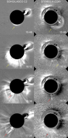 |
Fig. 1. Snapshots of coronagraphic observations using JHelioviewer (Müller et al. 2017). Left column: SOHO/LASCO C2 white-light base difference images. Right column: white-light base difference images from STEREO-A COR1. Yellow arrows indicate the CME and red arrows show the propagated leg of the filament eruption at time steps 16:36 UT and 17:36 UT, respectively. |
The EUV low coronal signatures of the CME were simultaneously observed by the SDO/AIA and STEREO-A/EUVI, separated by 37.6° in longitude at this date (see Fig. 2). The AIA instrument provides images of the Sun in seven EUV filters with a pixel scale of  over a FOV of about 1.3 R⊙. EUVI observes the Sun through four EUV passbands over a FOV up to 1.7 R⊙ providing images with a pixel scale of
  .
.
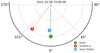 |
Fig. 2. View of the ecliptic plane showing the various spacecraft positions on 28 October 2021. SDO is located along the Sun–Earth line, while the STEREO-A and Solar Orbiter spacecraft are positioned 37.6° and 2.8° to the east, respectively. The image was generated using the Solar-MACH tool (Gieseler et al. 2023). |
For our analysis of coronal dimmings, we used AIA 193 Å filtergram images with a 12 s cadence. The selection of 193 Å for observing and extracting coronal dimmings is motivated by the systematic study of Dissauer et al. (2018b), demonstrating that this wavelength effectively captures both the quite and AR coronal plasma that is expelled during CMEs. The same images effectively resolve the filament propagation and we matched them with 2.5 min cadence sequences of 195 Å EUVI data for a 3D reconstruction of the filament. Both data series were calibrated and corrected for differential rotation to a reference time of 28 October 15:05 UT using the Sunpy library (The SunPy Community 2020) in Python. The detection and analysis procedures were also developed using Python.
Figure 3 gives an overview of the event as observed by the AIA original 193 Å filter showing direct images (left) and processed base-difference images (right). The coronal dimming, eruptive filament, and EUV wave are well observed in base difference data, originating at longitudes close to the disk center for the line of sight (LOS) from Earth. The dimming is detected from the earliest time steps, starting around 15:05 UT with quasi-circular propagation, which later dominates mostly to the southeast, reaching the neighboring active region. The filament eruption starts around 15:10−15:12 UT, propagating to the southeast and reaching off-limb at 15:47 UT. Another part of the filament is visible off-limb around 15:35 UT to the west. The EUV wave appears around 15:28 UT and is visible on the solar surface up to 15:50 UT, showing an initially quasi-circular propagation, with dense fronts toward the north (second and third panels, see also the online movie). Devi et al. (2022) presented a full analysis of the EUV wave evolution, reporting a maximum speed of its propagation of about 700 km s−1.
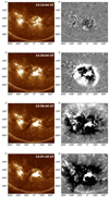 |
Fig. 3. Overview of the 28 October 2021 event, showing the dimming evolution and eruption of the filament in AIA 193 Å. Left: direct images. Right: corresponding base-difference images. Four time steps are shown, while the full evolution of the event can be found in the online movie. |
The associated X1.0 flare was also detected in hard X-rays (HXR) by the Spectrometer Telescope for Imaging X-rays (STIX; Krucker et al. 2020) on board Solar Orbiter. During the 28 October 2021 event, Solar Orbiter was close to the Sun–Earth line (2.8° east) at a distance of 0.80 AU from the Sun. As this was an X-class flare, STIX detected significant emission in both the thermal and nonthermal energy ranges, enabling insight into a broader range of the flare process. STIX uses a pair of grids to indirectly reconstruct images of the HXR photons by producing Moire fringes that deferentially illuminate different detector pixels. STIX images (Fig. 4) were produced in three energy bands: the thermally dominated 4−10 keV, the intermediate 15−25 keV, and the nonthermal 25−50 keV band. For context and comparison, these were overlaid on SDO AIA 171 Å and 1600 Å images after being rotated to the SDO point of view. In order to accurately perform the rotation of the STIX sources, estimates of the X-ray source heights must be made. For the nonthermal footpoints, we used the equation in Aschwanden et al. (2002) relating energy to height. For the thermal sources, we assumed a semi-circle connecting the two ribbons. As there was no STIX aspect solution for this time, we applied a small adjustment of [−40″, 5″] to align the STIX sources with the AIA ribbons. The STIX observations were corrected for the difference in light travel time (94.58 s) from the Sun to Solar Orbiter and from the Sun to Earth.
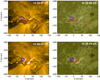 |
Fig. 4. STIX images showing 50%, 70%, and 90% contours for energy bands 4−10 keV (red), 15−25 keV (blue), and 25−50 keV (dark blue). The STIX contours are rotated to the point of view of SDO and overlaid on AIA images. The AIA images are shown for two different time steps: top row – 15:25 UT, and bottom row – 15:26 UT; and at two different AIA filters: left column – 171 Å, and right column – 1600 Å. |
3. Methods and results
Our approach consists of three steps. First, we developed a method for estimating the dominant direction of the dimming development (Sect. 3.1). Second, to determine the direction of parts of the erupting structure and flux rope during the early CME evolution, we performed 3D reconstructions of the eruptive filament (Sect. 3.2) and a 3D CME reconstruction using GCS modeling (Sect. 3.3). Finally, we studied the relation between the dominant dimming direction, the direction of the filament eruption, and the CME (Sect. 3.4).
3.1. Coronal dimming
Here, we present the method we used to estimate the dominant direction of the dimming development, which includes the dimming segmentation (Sect. 3.1.1), followed by our assessment of the evolution of the dimming area with the help of a sector analysis (Sect. 3.1.2).
3.1.1. Dimming segmentation
For the dimming segmentation and analysis, we used a sequence of AIA 193 Å maps within the 15:00−15:57 UT time range. As the dimming regions are characterized by a drop in EUV intensity, for their detection we created base-difference images, indicating the absolute change in the intensity values with respect to the pre-eruptive coronal state. We applied an automated detection technique based on thresholding and region growing to these images (similar to the one described in Dissauer et al. 2018b). First, we extracted all pixels where the intensity dropped below −30 DN. This level was selected empirically by qualitatively checking images during different development stages of the dimming in order to also include distant parts (see Fig. 3). Second, we used 30% of the darkest pixels of this set as seeds for the region-growing algorithm to connect all the separated parts of the dimming region. To minimize the noise, we used median filtering with a 3 × 3 kernel.
We obtained the dimming masks for all the time steps from 15:05 to 15:57 UT and united them into one cumulative dimming mask. This mask contains all pixels that have been flagged as dimming pixels during the chosen time range. However, pixels of the erupting filament also show up in the mask as they have a similar intensity level. To exclude these pixels, we used the same mask in a base-difference image at one of the last time steps (when the filament was already gone) and refined the mask by deleting all the pixels with intensity above −30 DN, subsequently filling the gaps within the contour. The final cumulative dimming mask (Fig. 5) was then used for further dimming analysis.
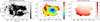 |
Fig. 5. Total area of the dimming region. Left: base-difference map at the time of maximal dimming extent at 15:57 UT. Middle: cumulative timing map of the whole dimming extraction, color-coded in minutes from 15:05 UT. Right: same dimming map, but each pixel shows the ratio of its area to the area of the average pixel in the center. Dashed curves and numbers represent the chosen sectors. |
3.1.2. Dimming sector analysis
To determine the main direction of the dimming expansion, we designed a spherical polar coordinate system centered at the source region and divided the solar surface into 16 angular sectors of Δϕ = 22.5° width (counted counterclockwise). The source location was defined in accordance with the center of the flare emission contours from STIX (Fig. 4). For each sector, we further calculated the integral area of all pixels by developing a method to estimate the surface area of a sphere for every pixel. In Appendix A, we present a comprehensive description of the area calculation, including a comparative analysis of sector areas derived from corrected pixels and their corresponding averages. All the code is publicly available on GitHub2.
Figure 5 (left panel) shows the dimming region at the times close to its maximal extent (similar to the end of the dimming impulsive phase described in Dissauer et al. 2018a), the cumulative dimming map, where each pixel is color-coded according to the time of its first detection (middle panel) and also according to the ratio of each corrected pixel area to the average (square) pixel area in the center of the Sun (right panel) for each sector.
We define the main direction of the overall dimming development as the middle longitude of the sector with the largest area. To estimate the uncertainty in the area due to a specific threshold used for the dimming segmentation, we additionally applied a ±5% change to the threshold level and computed the mean values and corresponding standard deviation of the dimming area in each sector. The resulting dimming areas for the different sectors together with the uncertainty ranges are shown in Fig. 6.
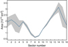 |
Fig. 6. Dimming area calculated for each sector in the full cumulative map. The shaded band indicates the error estimation using different threshold levels used for the dimming segmentation. The largest dimming area is in sector no. 14. |
As can be seen, the dimming dominates in the southern sectors with the largest area in sector no. 14. Furthermore, analyzing the cumulative timing map (the middle panel in Fig. 5), we observe a two-stage evolution of the dimming region. Initially, the dimming spreads around the source, as indicated by the presence of blue and green pixels indicating evolution until ≈15:35 UT. Subsequently, the southeastern part of the dimming region becomes more pronounced and dominates the overall expansion.
In this particular case, the use of one cumulative mask in the dimming segmentation instead of tracking the dimming region over time helps to include the dimming areas hidden by other coronal structures at different stages of their evolution; for example, those initially covered by flare loops. At the same time, we note that the sector analysis can also be successfully implemented on a sequence of dimming masks, which allows us to track the time evolution of characteristic dimming parameters (e.g., area/brightness/leading edge) during different parts of the dimming evolution with respect to the eruption source. The dominant direction of the dimming propagation can then be defined as the sector with the fastest dynamics; for example, with the highest area change rate for the particular time step.
3.2. Eruptive filament
Here, we present 3D reconstructions of the eruptive filament (Sect. 3.2.1) and study its kinematics (Sect. 3.2.2).
3.2.1. Three-dimensional reconstruction of the erupting filament
The dense and cool filament material is usually thought to be embedded in the dips of a magnetic flux rope, where the magnetic tension force keeps it in balance against the gravitational force. Therefore, the erupting filament can be analyzed in order to locate the inner part of the erupting flux rope during the early stages of the eruption. The use of dual-point EUV observations from SDO and STEREO-A allows us to perform the 3D reconstruction of the eruptive filament using an epipolar geometry approach (see full description in Inhester 2006; Podladchikova et al. 2019). A point on the object and two observer positions create an epipolar plane, which, by definition, is seen as an epipolar line in each of the observer’s images. At each time step, we manually identify the highest points of the filament from SDO/AIA 193 Å images and match these with the corresponding points on the epipolar lines located in STEREO-A/EUVI 195 Å data. Thus, for every point of the filament there is only one degree of freedom in placing the corresponding matching point in another image. In order to enhance the contrast of the erupting or moving features, we use base-difference images along with direct images for feature identification.
Figure 7 shows a sequence of SDO/AIA 193 Å (top) and STEREO-A/EUVI 195 Å (bottom) maps, where the colored markers highlight the propagation of the erupting filament based on matching the same features on both AIA (blue) and EUVI (red) images. We track the filament growth using direct images for the time steps 15:05−15:32 UT (a) and base-difference images for 15:35−15:57 UT (b). For each point of the filament, we obtain coordinates in the heliocentric Earth equatorial (HEEQ) coordinate system, defining its position in 3D.
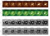 |
Fig. 7. Evolution of the erupting filament between 15:12 and 15:32 UT in SDO AIA 193 Å (top) and STEREO-A EUVI 195 Å direct images (a) and between 15:35 and 15:50 UT in base difference images (b). Blue markers show the upper tip of the filament observed by SDO AIA, and red markers indicate the matching points from the STEREO-A vantage point. Epipolar lines are shown in white. The yellow arrows indicate another, central part of the filament eruption. We note that the image scale of panels a and b is different. An animation of the reconstructions of panel b can be found in the online movie. |
We then determine the orthogonal projections of the reconstructed 3D points on the solar surface – which reflect the projected direction of the filament eruption – using the following equation:
 (1)
(1)
Here, XP, YP, and ZP denote the 3D cartesian coordinates of the orthogonal projection on the solar surface, RSun is the solar radius, and X, Y, and Z are the 3D coordinates of the reconstructed points of the filament.
Figure 8 represents the connection of the low coronal signatures (left panels) with the CME propagation further out (right panels). The left panels show snapshots of SDO/AIA 193 Å (top, 15:49:52 UT) and STEREO-A/EUVI 195 Å (bottom, 15:50:00 UT) with matching points of the eruptive filament (blue and red, respectively, the same points as in Fig. 7b) and their orthogonal projections on the surface (green for AIA and yellow for EUVI). A white grid shows the dimming sectors on the solar surface. Solar EUV images show only the filament projections along the LOS of the spacecraft, and, as can be seen from Fig. 8 (left panels), the LOS and the orthogonal (which is independent of the viewpoint) projections of the filament are located in different sectors. At the same time, the distance between the LOS and orthogonal projections is significantly greater for STEREO-A (bottom) than for SDO (top), as STEREO-A, positioned 37.6° east of Earth, reveals the location of the event in the southwestern quadrant of the hemisphere, whereas SDO gives a view of the event in the southern hemisphere close to the disk center. We note that the orthogonal projections of the filament are located in the sector with the largest area of dimming (no. 14).
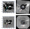 |
Fig. 8. Connection of the low coronal signatures with the CME propagation further out. Left panels: SDO AIA 193 Å and STEREO-A EUVI 195 Å base-difference images with reconstructed matching points of the eruptive filament (blue and red, respectively) and their orthogonal projections on the surface (green and yellow). The sector with the largest area of dimming is marked by its number (no. 14). Right panels: propagation of the CME seen from SOHO/LASCO C2 (top) and STEREO-A COR2 (bottom) coronagraphs at later time steps. Red arrows indicate the filament development as the bright substructure of the CME. Coronagraphic observations were obtained using JHelioviewer (Müller et al. 2017). |
The right panels of Fig. 8 show later observations of the CME propagation from SOHO/LASCO C2 (top) and STEREO-A COR2 (bottom) coronagraphs. This visual representation shows that the filament trajectory appears differently from these two viewpoints. The filament propagates almost as a straight line in the view from SDO. At the same time, STEREO observations reveal that a part of the filament structure decelerates and falls back to the solar surface.
To gain a deeper understanding of the filament trajectory, we calculate its deflection from the radial direction in 3D space. To do so, we define a linear fit to the filament points constrained to the first reconstructed point with the lowest height. The angle between the linear fit and the radial direction is 54°. SDO/STEREO observations allowed us to reconstruct only one “leg” of the filament (the eastern one), whereas the coronagraphic observations indicate another filament part, appearing earlier. Xu et al. (2022) also revealed this double structure of the eruption and estimated the velocities of the other part. We additionally analyzed the deflection of the filament propagation from radial by splitting the angle of deflection into two components. To this end, we projected the linear fit and radial direction onto equatorial and meridional planes and calculated the 2D angles between projections in each plane. Both vectors (dark red and black lines, respectively) with their projections (dashed lines) are presented in Fig. 9. We derive that the linear fit to the filament points is declined from radial by 64° (yellow arc) to the east and by 38° (two red arcs) to the south.
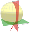 |
Fig. 9. Three-dimensional model of the Sun with the reconstructed filament. Red points show the reconstructed heights of the filament. The dark red line shows a linear fit and the red dashed lines represent projections onto equatorial (green) and meridional (red) planes. The black line indicates the radial direction, and the dashed black line shows its projection onto the equatorial plane. Equatorial and meridional planes both go through the intersection of the linear fit with the solar surface (filament origin). The radial direction is located in the meridional plane by definition. For clarity, the heliocentric coordinates grid is shown in gray. The inclination angle from the radial in the equatorial plane is shown as a yellow arc, and the inclination angle in the meridional plane is shown as two red arcs, respectively. |
3.2.2. Kinematics of the erupting filament
From the 3D reconstructions of the upper tip of the filament identified in each frame, we estimate its height and speed. Figure 10 shows the time evolution of the height (a), speed (b), and acceleration (c) of the filament in comparison to the GOES soft X-ray (SXR) flux evolution of the associated flare and its change rate (d) and the STIX hard X-ray count rates at different energies (e). In the panel a we show the resulting filament heights with black dots, while the error bar represents a ±5 pixel shift in the AIA images in finding the matching point along the epipolar line. To obtain the filament velocity and acceleration profiles, we first smooth the filament height data and obtain the first and second direct numerical derivatives. The smoothing technique which Podladchikova et al. (2017) present and extend to nonequidistant data optimizes between two criteria in order to find a balance between data fidelity and smoothness of the approximating curve (see also the applications in Veronig et al. 2018; Dissauer et al. 2019; Gou et al. 2020; Saqri et al. 2023). Using the derived acceleration profile, we then interpolate to equidistant data points (solid line in c panel) based on the minimization of the second derivatives and reconstruct the corresponding velocity (solid line in b panel) and height (solid line in a panel) profiles by integration. We also obtain the errors of kinematic profiles by representing the reconstructed filament height, velocity, and acceleration as an explicit function of original errors of filament height-time data (blue shaded areas). The dots in panels b and c give the first and second time derivatives obtained directly from the height measurements. As the eruption evolves, the upper filament parts start to become fainter from around 15:40 UT. Therefore, at later stages of observation, we may not be able to accurately identify the highest points of the filament, but instead only the lower ones located further inside it. Consequently, the measured heights and velocities at these times may be underestimated. In panel d, we calculate the change rate of the GOES SXR flux as the first-order numerical derivative and smooth by a forward-backward exponential smoothing method (Brown 1963). As can be seen from Fig. 10, the height of the filament increases up to 312 ± 5 Mm within 37 min with a maximum speed of ≈250 km s−1. The filament shows a slow rise from 15:12 until 15:25 UT, and then rapidly accelerates to ≈366 m s−2, reaching 52 Mm at 15:28 UT with a further gradual increase in speed. The peak of acceleration is cotemporal with peaks in the high-energy STIX curve and a rapid increase in GOES flux. The overall evolution of the filament speed profile precedes the associated flare flux: the flare started at ≈15:17 UT, reached its maximum around 15:35 UT, and then entered a phase of decline.
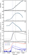 |
Fig. 10. Kinematics of the erupting filament and associated SXR flare evolution. (a) Height estimations of the filament (black markers). The error bar presents the five-pixel shift in finding the matching point along the epipolar line. The corresponding black solid line indicates the smoothed height-time profile. (b) Speed and (c) acceleration of the filament obtained by numerical differentiation of height-time data (dots) and smoothed profiles (lines). The shaded areas give the error ranges. (d) GOES 1−8 Å SXR light curve (black curve, left Y-axis) and the corresponding change rate (gray curve, right Y-axis). (e) STIX count rates at 4−10 keV (red), 15−25 keV (blue), and 25−50 keV (dark blue) energies. The vertical dashed lines mark the peaks in the 25−50 keV STIX curve (dark blue), the GOES SXR flux (black), and its derivative (gray). |
3.3. GCS reconstruction of the CME
We also analyzed the associated 3D CME structure and direction using the GCS model applied to the SOHO/LASCO C2 and STEREO-A/COR2 coronagraph data, which have a FOV out to 6 R⊙ and 15 R⊙, respectively. The top panels in Fig. 11 show the observations of the CME by STEREO-A COR2 (left) and SOHO/LASCO C2 (right) coronagraphs. The bottom panels show the best fit (green mesh) resulting from the GCS 3D flux rope model when requiring that the boundary of the GCS model flux rope match the outer edge of the CME shape in COR2 (left) and LASCO (right) white-light images.
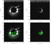 |
Fig. 11. Observations of the CME by SOHO/LASCO C2 (left) and STEREO-A COR2 (right) coronagraphs with the GCS reconstructions (green mesh). |
We obtain the following parameters of this reconstruction: heliocentric longitude lon = 357°, heliocentric latitude lat = −30°, height corresponding to the apex of the croissant h = 6 R⊙, tilt of the croissant axis to the solar equatorial plane tilt = 15°, half-angle measured between the apex and the central axis of a leg of the croissant α/2 = 60°, and aspect ratio r = 0.5. The footprint positions of the croissant are located at [299° , − 46°] and [55° , − 14°]. As can be seen from Fig. 11, the CME according to GCS reconstructions propagates almost radially in the southeastern direction.
3.4. Relationship between dimming, filament, and CME directivity
Using the Python code provided in von Forstner (2021), we plotted the GCS structure on the 3D model of the Sun to compare it with the coronal dimming. Figure 12 reveals a match between the total dimming region (blue contour) and the reconstructed shape and direction of the CME, represented by the GCS croissant (green mesh). Notably, the dimming contour precisely aligns with the inner portion (blue mesh) located between the two footpoints of the GCS croissant. Our tracking of the dimming region extends from 15:00 UT up to 15:57 UT, while the CME structure was reconstructed for 16:12 UT. Assuming the CME propagates without deflection during this time span, our observations strongly suggest a spatial association between these features. To investigate this association more thoroughly, we compare both structures on the solar surface using the orthogonal projection of the inner part (the closest one to the solar surface) and the location of the primary axis of GCS.
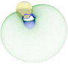 |
Fig. 12. Three-dimensional model of the Sun with the GCS croissant (green mesh with blue inner part) and coronal dimming (blue contour). |
Figure 13 shows an AIA 193 Å image with the total cumulative dimming area (blue contour) and the projected inner part of the GCS reconstruction (green mesh). We mark the source point of the primary axis of the GCS croissant with a green marker. As can be seen, the projections (green) are mainly concentrated in the center of the dimming, which allows us to link the 2D dimming with the 3D CME bubble. To explore this further, we also determined the center of mass of the dimming (red marker in Fig. 13). For each pixel, we consider its position vector ri = (xi, yi) and associate it with a weight ai, where i = 1, 2, …, n. The center of mass, denoted rcm, is then computed using the formula:
 (2)
(2)
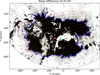 |
Fig. 13. AIA 193 Å base difference image showing the dimming region (blue contour) with an overlaid orthogonal projection of the inner part of the GCS bubble (green mesh). The green marker indicates the source location derived from the GCS reconstruction, and the red marker represents the center of mass of the dimming region. The red mesh illustrates the orthogonal projection of the inner part of the GCS reconstruction, with the source point shifted to the location of the center of mass. |
Here, the weight of each pixel corresponds to its area on the solar surface. Consequently, the larger the area, the more significant its contribution to the overall dimming morphology. By analyzing the coordinates of the center of mass, we gain insights into the propagation of the dimming relative to the eruption source (flare coordinate) and can compare it to the primary axis footpoint of the GCS croissant. The center of mass for the dimming has a heliographic longitude of loncm = −8° and a heliographic latitude of latcm = −28.8° and lies within the sector associated with the dominant dimming propagation. The center of mass is located 5° to the west and 1.2° to the north from the location of the primary axis of the GCS, which is within the uncertainty range of the reconstruction.
We further create a modified GCS croissant with the same parameters but with a shifted primary axis to align with the center of mass of the dimming area. The orthogonal projection of this adjusted croissant is illustrated in Fig. 13 with red mesh. The full GCS croissant (green) with its shifted version (red) almost align in the SOHO/LASCO 16:12 UT coronagraph image (Fig. 14). Consequently, the center of mass can serve as an additional validation measure for obtaining the CME direction.
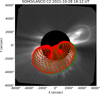 |
Fig. 14. Comparison of the two versions of the GCS reconstruction on the SOHO/LASCO C2 16:12 UT image of the CME. The green mesh represents the GCS reconstruction from coronagraph observations, and the red mesh represents the same croissant with a changed location of source chosen by the dimming center of mass. |
Figure 15 combines all results of our event analysis in one visualization of the studied eruptive features, shown from SDO and STEREO-A perspectives: the dimming region (blue contour) with the dominant dimming direction (filled sector), the reconstructed 3D filament motion (red points) with their orthogonal projections (purple points), and the modeled CME according to GCS reconstructions (the inner part of the GCS bubble is shown as blue mesh, the main axis as a green vector). The dark red line shows a linear fit to the reconstructed 3D filament points constrained to the first reconstructed point with the lowest height.
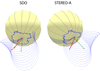 |
Fig. 15. Three-dimensional model of the Sun observed from SDO (left) and STEREO-A (right). The dimming borders are shown with blue contours and the sectors are drawn as light blue lines (the filled area indicates the sector of dominant dimming propagation). Red points mark the reconstructed filament heights, and purple points are their orthogonal projections on the surface. The inner part of the GCS reconstruction is plotted as blue mesh. The dark red line presents the straight line fit to the reconstructed filament positions. The green line shows the axis of the CME, which is represented by the GCS croissant. |
With this visual representation, for the first time we can directly compare and relate the dimming evolution, the filament eruption, and the CME propagation to one another:
-
The orthogonal projections of the erupting filament, which reflect the projected motion of this structure onto the solar surface, are located in the same sector as the dominant direction of the dimming evolution. Orthogonal projections are independent of the observation point, allowing us to establish a link between the 3D direction vector and the evolution of the dimming area on the solar surface. Consequently, the morphology of the coronal dimming serves as a reliable indicator of motion of the lower-lying signatures associated with the eruption of the flux rope.
-
Despite the prevailing southwestern direction of the dimming propagation, it is important to consider the comprehensive dimming morphology, which also exhibits its widespread evolution around the eruption source. A compelling correspondence can be observed between the total dimming region and the reconstructed shape and direction of the CME. Specifically, the dimming contour reflects the inner part of the GCS croissant, indicating their spatial association.
-
The angle between the fit to the reconstructed filament height evolution and the apex of the GCS croissant is 50°. This value roughly matches with the CME half-width parameter of the GCS reconstruction (α/2 = 60°), which represents the angle between the apex and the leg of the CME croissant. This similarity suggests that the reconstructed filament can be reasonably associated with the eastern leg of the GCS croissant, indicating a notable correspondence between the two structures.
4. Discussion and conclusions
In this paper, we present a detailed analysis of the different features involved in the eruption of the 28 October 2021 X1.0 event, namely the erupting filament, the CME, and the coronal dimming evolution. Our research involves the reconstruction of both the low-lying filament eruption and the CME structure at a height of 6 R⊙ in order to determine the direction of the initial flux rope propagation in 3D space. Simultaneously, we define the dominant propagation of the dimming growth based on an assessment of the evolution of the dimming area and the sector analysis on the solar surface. To compare the directions, we calculated the orthogonal projections of the reconstructed points (both filament and GCS), which enabled us to track their motion projected onto the solar surface.
We developed a method to estimate the dominant direction of the dimming development based on our assessment of the evolution of the dimming area using sector analysis. Initially, the dimming expansion spreads symmetrically around the source region; subsequently, it undergoes further development toward the southeast. The sector analysis of the cumulative dimming area clearly indicates that the dominant direction of total dimming growth aligns with one of the southeastern sectors.
As we consider the dimming region on the solar sphere, we introduce a novel technique that involves identifying the surface area for each pixel. This approach effectively minimizes projection effects, as it takes into account the spherical projection of each individual pixel of the dimming area. We made the code for the calculation of the correction publicly available on GitHub.
A filament was observed both by SDO and STEREO-A up to ≈312 Mm in height, which allowed us to reconstruct its evolution in 3D. The erupting filament starts to rise at a slow speed at ≈15:12 UT, and then rapidly accelerates between ≈15:25 and 15:30 UT, which coincides with a phase during which the flare rises in the GOES 1−8 Å SXR flux, while the filament impulsive acceleration occurs co-temporally with the STIX high-energy hard X-ray emission at 15−25 keV and 25−50 keV (see Fig. 10). The maximum speed and acceleration of the erupting filament area ≈250 km s−1 and ≈366 m s−2, respectively. A similar filament evolution was also reported in Devi et al. (2022), where the time–distance plots of the filament heights in 2D were used to derive the height and kinematics profiles. These authors also report a nonlinear acceleration at the same range, which they relate to the presence of torus instability in the eruption behavior.
The reconstructed filament heights projected to the solar surface coincide with the dominant direction of the dimming expansion. This allows us, for the first time, to make a direct comparison of the dimming and filament directions within a unified coordinate system. We find that the dimming precisely reflects the propagation of the filament eruption low in the corona.
The significant inclination between the motion of the 3D filament and the radial direction (64° to the east and 38° to the south) reveals a double structure of the flux rope. Both filament parts are observed as the brightest and densest CME material in the coronagraph images (Fig. 8, right panels). By modeling the propagation of the flux rope using GCS reconstruction, we find that the CME primarily propagates radially in the southeastern direction. We obtain a deviation of 50° between the direction of the CME and the erupting filament. This indicates that the portion of the filament used for the 3D reconstruction, which is clearly observed, does not correspond to the apex of the CME flux rope. Instead, it is associated with one of the legs of the flux rope. In addition, the close agreement between the deviation angle value and the half-width parameter of the GCS reconstruction (α/2 = 60°) further supports the correspondence between the reconstructed filament and the eastern leg of the GCS croissant.
The strongly nonradial behavior of the erupting filament obtained from the 3D reconstruction may also indicate a pronounced lateral expansion of the flux rope, which contrasts with the assumption of self-similar propagation in the GCS reconstruction of the CME. This would lead to nonradial propagation of the CME leg, even if its apex is propagating radially. Hovis-Afflerbach et al. (2023) also discussed whether the evolution of the filament in the low corona can be used as a predictor of CME direction, as observed in coronagraph data.
We observed distinct signatures of both components of the flux rope in the evolution of the dimming region. While the dominant propagation of the dimming follows a southwestern direction, reflecting the filament evolution, it is important to acknowledge the comprehensive morphology of the dimming, which shows an extensive evolution around the eruption source. Our analysis reveals a compelling relation between the total dimming region and the reconstructed shape and direction of the CME. Specifically, the dimming contour closely aligns with the inner part of the GCS croissant, while the center of mass of the dimming region is situated in close proximity to the projection of the primary axis of the GCS reconstruction, indicating a clear spatial association between the dimming and the CME.
At the same time, in our case study, we do not find the direction of the filament eruption to be directly related to the direction of the CME expansion, evidenced by a significant deviation angle between the reconstructed filament heights and the CME (GCS) axis. The filament material is lying in the lower portion of the expanding flux rope (Cheng et al. 2014). With that, we point out that the filament itself cannot always be used as a reliable proxy to predict the main direction of CME propagation.
These findings highlight that the evolution of the dimmings reflects both the direction of a low-lying erupting magnetic structure (filament) and the global propagation of CMEs. Further research efforts need to consider both the dominant dimming direction and the dimming morphology in order to understand the link between 2D dimming information and the initial 3D direction of the CME/flux rope and therefore enhance our understanding of its early dynamics.
Movies
Movie 1 associated with Fig. 3 (overview) Access Supplementary Material
Movie 2 associated with Fig. 7 (Reconstruction) Access Supplementary Material
Acknowledgments
G.C. and T.P. acknowledge support from the Russian Science Foundation under the project 23-22-00242. K.D. acknowledges support from NASA under award No. 80NSSC21K0738 and the NSF under AGS-ST Grant 2154653. A.M.V. and E.C.M.D. acknowledge the Austria Science Fund (FWF): project no. 14555-N. M.D. acknowledges the support by the Croatian Science Foundation under the project IP-2020-02-9893 (ICOHOSS). SDO data are courtesy of the NASA/SDO AIA and HMI science teams. The SOHO/LASCO data used here are produced by a consortium of the Naval Research Laboratory (USA), Max-Planck-Institut für Aeronomie (Germany), Laboratoire d’Astronomie (France), and the University of Birmingham (UK). The STEREO/SECCHI data are produced by an international consortium of the Naval Research Laboratory (USA), Lockheed Martin Solar and Astrophysics Lab. (USA), NASA Goddard Space Flight Center (USA), Rutherford Appleton Laboratory (UK), University of Birmingham (UK), Max-Planck-Institut für Sonnenforschung (Germany), Centre Spatiale de Liège (Belgium), Institut d’Optique Théorique et Appliquée (France), and Institut d’Astrophysique Spatiale (France). Solar Orbiter is a mission of international cooperation between ESA and NASA, operated by ESA. We thank the referee for valuable comments on this study.
References
- Aschwanden, M. J. 2016, ApJ, 831, 105 [NASA ADS] [CrossRef] [Google Scholar]
- Aschwanden, M. J., Brown, J. C., & Kontar, E. P. 2002, Sol. Phys., 210, 383 [Google Scholar]
- Bronshtein, I. N., Semendyayev, K. A., Musiol, G., & Muehlig, H. 2007, Handbook of Mathematics (Berlin, Heidelberg: Springer), 1164 [Google Scholar]
- Brown, R. G. 1963, Smoothing Forecasting and Prediction in Discrete Time Series (New Jersey: Prentice Hall), 468 [Google Scholar]
- Burkepile, J. T., Hundhausen, A. J., Stanger, A. L., St. Cyr, O. C., & Seiden, J. A. 2004, J. Geophys. Res.: Space Phys., 109, A03103 [NASA ADS] [CrossRef] [Google Scholar]
- Byrne, J. P., Maloney, S. A., McAteer, R. J., Refojo, J. M., & Gallagher, P. T. 2010, Nat. Commun., 1, 74 [NASA ADS] [CrossRef] [Google Scholar]
- Cheng, X., Ding, M. D., Guo, Y., et al. 2014, ApJ, 780, 28 [Google Scholar]
- Cheng, X., Guo, Y., & Ding, M. 2017, Sci. China Earth Sci., 60, 1383 [Google Scholar]
- Chertok, I., & Grechnev, V. 2003, Astron. Rep., 47, 934 [NASA ADS] [CrossRef] [Google Scholar]
- Chikunova, G., Dissauer, K., Podladchikova, T., & Veronig, A. M. 2020, ApJ, 896, 17 [NASA ADS] [CrossRef] [Google Scholar]
- Darnel, J. M., Seaton, D. B., Bethge, C., et al. 2022, Space Weather, 20, e2022SW003044 [CrossRef] [Google Scholar]
- Devi, P., Chandra, R., Awasthi, A. K., Schmieder, B., & Joshi, R. 2022, Sol. Phys., 297, 153 [NASA ADS] [CrossRef] [Google Scholar]
- Dissauer, K., Veronig, A. M., Temmer, M., Podladchikova, T., & Vanninathan, K. 2018a, ApJ, 863, 169 [NASA ADS] [CrossRef] [Google Scholar]
- Dissauer, K., Veronig, A. M., Temmer, M., Podladchikova, T., & Vanninathan, K. 2018b, ApJ, 855, 137 [NASA ADS] [CrossRef] [Google Scholar]
- Dissauer, K., Veronig, A. M., Temmer, M., & Podladchikova, T. 2019, ApJ, 874, 123 [NASA ADS] [CrossRef] [Google Scholar]
- Downs, C., Roussev, I. I., van der Holst, B., Lugaz, N., & Sokolov, I. V. 2012, ApJ, 750, 134 [NASA ADS] [CrossRef] [Google Scholar]
- Dumbović, M., Veronig, A. M., Podladchikova, T., et al. 2021, A&A, 652, A159 [NASA ADS] [CrossRef] [EDP Sciences] [Google Scholar]
- Gieseler, J., Dresing, N., Palmroos, C., et al. 2023, Front. Astron. Space Sci., 9, 384 [NASA ADS] [CrossRef] [Google Scholar]
- Gopalswamy, N., Lara, A., Lepping, R., et al. 2000, Geophys. Res. Lett., 27, 145 [NASA ADS] [CrossRef] [Google Scholar]
- Gopalswamy, N., Yashiro, S., Michalek, G., et al. 2009, Earth Moon Planets, 104, 295 [NASA ADS] [CrossRef] [Google Scholar]
- Gou, T., Veronig, A. M., Liu, R., et al. 2020, ApJ, 897, L36 [NASA ADS] [CrossRef] [Google Scholar]
- Guo, J., Ni, Y., Zhong, Z., et al. 2023, ApJS, 266, 3 [NASA ADS] [CrossRef] [Google Scholar]
- Hagenaar, H. J. 2001, ApJ, 555, 448 [NASA ADS] [CrossRef] [Google Scholar]
- Harra, L. K., & Sterling, A. C. 2001, ApJ, 561, L215 [CrossRef] [Google Scholar]
- Harrison, R. 1995, A&A, 304, 585 [NASA ADS] [Google Scholar]
- Harrison, R. A., & Lyons, M. 2000, A&A, 358, 1097 [NASA ADS] [Google Scholar]
- Heinemann, S. G., Temmer, M., Farrugia, C. J., et al. 2019, Sol. Phys., 294, 121 [NASA ADS] [CrossRef] [Google Scholar]
- Hou, Z., Tian, H., Wang, J.-S., et al. 2022, ApJ, 928, 98 [NASA ADS] [CrossRef] [Google Scholar]
- Hovis-Afflerbach, B. A., Thompson, B. J., & Mason, E. I. 2023, Space Weather, 21, e2022SW003256 [NASA ADS] [CrossRef] [Google Scholar]
- Howard, T. A., DeForest, C. E., Schneck, U. G., & Alden, C. R. 2017, ApJ, 834, 86 [NASA ADS] [CrossRef] [Google Scholar]
- Hudson, H. S., Acton, L. W., & Freeland, S. L. 1996, ApJ, 470, 629 [CrossRef] [Google Scholar]
- Hughes-Hallett, D., McCallum, W. G., Gleason, A. M., et al. 2017, Handbook of Mathematics (Berlin, Heidelberg: Springer), 592 [Google Scholar]
- Illing, R. M. E., & Hundhausen, A. J. 1986, J. Geophys. Res., 91, 10951 [Google Scholar]
- Inhester, B. 2006, ArXiv e-prints [arXiv:astro-ph/0612649] [Google Scholar]
- Kaiser, M. L., Kucera, T. A., Davila, J. M., et al. 2008, Space Sci. Rev., 136, 5 [Google Scholar]
- Kazachenko, M. D., Albelo-Corchado, M. F., Tamburri, C. A., & Welsch, B. T. 2022, Sol. Phys., 297, 59 [NASA ADS] [CrossRef] [Google Scholar]
- Klein, K.-L., Musset, S., Vilmer, N., et al. 2022, A&A, 663, A173 [CrossRef] [EDP Sciences] [Google Scholar]
- Koskinen, H. E. J., Baker, D. N., Balogh, A., et al. 2017, Space Sci. Rev., 212, 1137 [Google Scholar]
- Krista, L. D., & Reinard, A. A. 2017, ApJ, 839, 50 [NASA ADS] [CrossRef] [Google Scholar]
- Krucker, S., Hurford, G. J., Grimm, O., et al. 2020, A&A, 642, A15 [NASA ADS] [CrossRef] [EDP Sciences] [Google Scholar]
- Lemen, J. R., Title, A. M., Akin, D. J., et al. 2012, Sol. Phys., 275, 17 [Google Scholar]
- Li, T., & Zhang, J. 2013, ApJ, 770, L25 [NASA ADS] [CrossRef] [Google Scholar]
- Liewer, P. C., de Jong, E. M., Hall, J. R., et al. 2009, Sol. Phys., 256, 57 [Google Scholar]
- Liewer, P. C., Hall, J. R., Howard, R. A., et al. 2011, J. Atmos. Solar-Terr. Phys., 73, 1173 [NASA ADS] [CrossRef] [Google Scholar]
- Liu, Y., Thernisien, A., Luhmann, J. G., et al. 2010, ApJ, 722, 1762 [Google Scholar]
- López, F. M., Cremades, M. H., Nuevo, F. A., Balmaceda, L. A., & Vásquez, A. M. 2017, Sol. Phys., 292, 6 [CrossRef] [Google Scholar]
- Low, B. C., & Hundhausen, J. R. 1995, ApJ, 443, 818 [NASA ADS] [CrossRef] [Google Scholar]
- Mandrini, C. H., Nakwacki, M. S., Attrill, G., et al. 2007, Sol. Phys., 244, 25 [NASA ADS] [CrossRef] [Google Scholar]
- Mason, J. P., Woods, T. N., Webb, D. F., et al. 2016, ApJ, 830, 20 [NASA ADS] [CrossRef] [Google Scholar]
- Mason, J. P., Chamberlin, P. C., Seaton, D., et al. 2021, J. Space Weather Space Clim., 11, 20 [NASA ADS] [CrossRef] [EDP Sciences] [Google Scholar]
- Mierla, M., Davila, J., Thompson, W., et al. 2008, Sol. Phys., 252, 385 [NASA ADS] [CrossRef] [Google Scholar]
- Mierla, M., Inhester, B., Antunes, A., et al. 2010, Ann. Geophys., 28, 203 [NASA ADS] [CrossRef] [Google Scholar]
- Moran, T. G., & Davila, J. M. 2004, Science, 305, 66 [Google Scholar]
- Möstl, C., Rollett, T., Frahm, R. A., et al. 2015, Nat. Commun., 6, 7135 [CrossRef] [Google Scholar]
- Müller, D., Nicula, B., Felix, S., et al. 2017, A&A, 606, A10 [Google Scholar]
- Müller, D., St. Cyr, O. C., Zouganelis, I., et al. 2020, A&A, 642, A1 [Google Scholar]
- Papaioannou, A., Kouloumvakos, A., Mishev, A., et al. 2022, A&A, 660, L5 [NASA ADS] [CrossRef] [EDP Sciences] [Google Scholar]
- Pesnell, W. D., Thompson, B. J., & Chamberlin, P. C. 2012, Sol. Phys., 275, 3 [Google Scholar]
- Podladchikova, T., Van der Linden, R., & Veronig, A. M. 2017, ApJ, 850, 81 [NASA ADS] [CrossRef] [Google Scholar]
- Podladchikova, T., Veronig, A. M., Dissauer, K., Temmer, M., & Podladchikova, O. 2019, ApJ, 877, 68 [NASA ADS] [CrossRef] [Google Scholar]
- Prasad, A., Dissauer, K., Hu, Q., et al. 2020, ApJ, 903, 129 [Google Scholar]
- Pulkkinen, T. 2007, Liv. Rev. Sol. Phys., 4, 1 [Google Scholar]
- Rochus, P., Auchère, F., Berghmans, D., et al. 2020, A&A, 642, A8 [NASA ADS] [CrossRef] [EDP Sciences] [Google Scholar]
- Saqri, J., Veronig, A. M., Dickson, E. C. M., et al. 2023, A&A, 672, A23 [NASA ADS] [CrossRef] [EDP Sciences] [Google Scholar]
- Sterling, A. C., & Hudson, H. S. 1997, ApJ, 491, L55 [Google Scholar]
- Susino, R., Bemporad, A., & Dolei, S. 2014, ApJ, 790, 25 [NASA ADS] [CrossRef] [Google Scholar]
- Temmer, M. 2021, Liv. Rev. Sol. Phys., 18, 4 [NASA ADS] [CrossRef] [Google Scholar]
- Temmer, M., Veronig, A. M., Gopalswamy, N., & Yashiro, S. 2011, Sol. Phys., 273, 421 [NASA ADS] [CrossRef] [Google Scholar]
- Temmer, M., Thalmann, J. K., Dissauer, K., et al. 2017, Sol. Phys., 292, 93 [NASA ADS] [CrossRef] [Google Scholar]
- Thalmann, J. K., Dumbović, M., Dissauer, K., et al. 2023, A&A, 669, A72 [NASA ADS] [CrossRef] [EDP Sciences] [Google Scholar]
- The SunPy Community (Barnes, W. T., et al.) 2020, ApJ, 890, 68 [Google Scholar]
- Thernisien, A. 2011, ApJS, 194, 33 [Google Scholar]
- Thernisien, A. F. R., Howard, R. A., & Vourlidas, A. 2006, ApJ, 652, 763 [Google Scholar]
- Thompson, W. 2006, A&A, 449, 791 [NASA ADS] [CrossRef] [EDP Sciences] [Google Scholar]
- Thompson, B. J., Plunkett, S. P., Gurman, J. B., et al. 1998, Geophys. Res. Lett., 25, 2465 [Google Scholar]
- Thompson, B. J., Cliver, E. W., Nitta, N., Delannée, C., & Delaboudinière, J.-P. 2000, Geophys. Res. Lett., 27, 1431 [NASA ADS] [CrossRef] [Google Scholar]
- Tian, H., McIntosh, S. W., Xia, L., He, J., & Wang, X. 2012, ApJ, 748, 106 [NASA ADS] [CrossRef] [Google Scholar]
- Vanninathan, K., Veronig, A. M., Dissauer, K., & Temmer, M. 2018, ApJ, 857, 62 [NASA ADS] [CrossRef] [Google Scholar]
- Veronig, A. M., Podladchikova, T., Dissauer, K., et al. 2018, ApJ, 868, 107 [NASA ADS] [CrossRef] [Google Scholar]
- Veronig, A. M., Gömöry, P., Dissauer, K., Temmer, M., & Vanninathan, K. 2019, ApJ, 879, 85 [NASA ADS] [CrossRef] [Google Scholar]
- Veronig, A. M., Odert, P., Leitzinger, M., et al. 2021, Nat. Astron., 5, 697 [NASA ADS] [CrossRef] [Google Scholar]
- von Forstner, J. L. F. 2021, https://doi.org/10.5281/zenodo.5084818 [Google Scholar]
- Vourlidas, A., Lynch, B. J., Howard, R. A., & Li, Y. 2013, Sol. Phys., 284, 179 [NASA ADS] [Google Scholar]
- Webb, D. F., & Howard, T. A. 2012, Liv. Rev. Sol. Phys., 9, 1 [Google Scholar]
- Wills-Davey, M., & Attrill, G. D. R. 2009, AAS/Solar Physics Division Meeting, 40, 17.08 [NASA ADS] [Google Scholar]
- Wuelser, J. P., Lemen, J. R., Tarbell, T. D., et al. 2004, in Telescopes and Instrumentation for Solar Astrophysics, eds. S. Fineschi, & M. A. Gummin, SPIE Conf. Ser., 5171, 111 [NASA ADS] [CrossRef] [Google Scholar]
- Xu, Y., Tian, H., Hou, Z., et al. 2022, ApJ, 931, 76 [NASA ADS] [CrossRef] [Google Scholar]
- Zarro, D. M., Sterling, A. C., Thompson, B. J., Hudson, H. S., & Nitta, N. 1999, ApJ, 520, L139 [NASA ADS] [CrossRef] [Google Scholar]
- Zhang, Q. 2021, A&A, 653, L2 [NASA ADS] [CrossRef] [EDP Sciences] [Google Scholar]
Appendix A: Pixel area calculation
The method to define the main direction of the dimming propagation described in this work strongly relies on the dimming area parameter. The images of the Sun provide only a 2D representation of the actual 3D solar surface. Projection effects lead to the different weights of each pixel; e.g., closer to the limb, the pixel area is larger than for pixels closer to the Sun center. Therefore, for an accurate definition of the area, we present a method to identify the surface area of a sphere for each pixel.
The equation of the sphere is given by
 (A.1)
(A.1)
Here, R is the radius of the sphere in kilometers, and (x, y, z) are the coordinates of points of a sphere. The surface of a sphere can be described as a function of two variables:
 (A.2)
(A.2)
The projection of the sphere onto the XY plane is a circle belonging to the XOY plane, where O is the center of the sphere. The surface area of a sphere that has the region S as its projection onto the XOY plane is given by (Bronshtein et al. 2007)
 (A.3)
(A.3)
As follows from Equation (A.2),
 (A.4)
(A.4)
Therefore, using Equation (A.4), Equation (A.3) can be rewritten as
 (A.5)
(A.5)
Further, we present how to estimate the surface area of a sphere, where projection S onto the XOY plane has a size of 1 pixel. Figure A.1 shows the scheme of a solar image, where the outer square shows the boundaries of a solar image from a spacecraft. The marker C in the top left corner indicates the pixel with the coordinates (1,1), and i and j mark row and column numbers. The marker C′ also shows the pixel with the coordinates (1,1), but in a new coordinate system with rows i′ and columns j′ derived from i and j in the following way:
 (A.6)
(A.6)
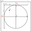 |
Fig. A.1. Scheme of a solar image. The outer square shows the boundaries of a solar image from a spacecraft. The marker C at the top left corner indicates the pixel with the coordinates (1,1), i - row number, j - column number. The marker C’ also shows the pixel with the coordinates (1,1), but in a new coordinate system with rows i′ and columns j′ connected to i and j via Equation (A.6). “Top”/“Left” show the distance (in pixels) from the top/left border of the image to the beginning of the Sun. P is a pixel, and |

Here, the Top/Left show the distance (in pixels) from the top/left border of the image to the beginning of the Sun. P is a pixel the area of which we are estimating, and  are the coordinates of its center. Pixel P is a square with a side a, the size of which is defined as
 (A.7)
(A.7)
Here, R is the radius of the Sun in kilometers, RP is radius of the Sun in pixels.
A coordinate Y of the lower pixel boundary is defined by
 (A.8)
(A.8)
A coordinate Y of the upper pixel boundary is given by
 (A.9)
(A.9)
A coordinate X of the left pixel boundary is determined as
 (A.10)
A coordinate X of the right pixel boundary is defined by
 (A.11)
Taking into account Equations (A.8–A.11), and replacing the calculation of the double integral by the successive calculation of two simple integrals, Equation (A.5) can be rewritten as
 (A.12)
Further, we solve the internal integral from Equation (A.12) analytically and the external one numerically. The internal integral from Equation (A.12) can be rewritten as
 (A.13)
Let us use the change of variables in Equation (A.13):
 (A.14)
Thus, Equation (A.13) can be rewritten as
 (A.15)
The solution of the integral represented by Equation (A.15) is given by
 (A.16)
Further, we solve the external integral of the resulting function given by Equation (A.16) using the mean rectangle method (Hughes-Hallett et al. 2017). First, we divide the integration interval by N regions:
 (A.17)
Here, N = 1000. Then we calculate the integral by finding a sum of the areas of N rectangles defined by
 (A.18)
Here, k = 1, 2, ⋯, N; Ak is calculated at the middle of each region, and x(k) takes the values within integration limits from a(−RP + j′−0.5) to a(−RP + j′+0.5) and for each k is estimated as
 (A.19)
The resulting area of a pixel is defined by the sum of xk.
With this method, we calculate the area of every pixel of the solar disk and construct a correction map, where each pixel is weighted by its area (Figure A.2). The color bar shows the ratio of each pixel area to the square pixel in the center of the solar disk. Any mask of the dimming region can be applied to this map to obtain the final dimming area; the corrected dimming mask for the 2021 October 28 event is shown in Figure 5.
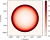 |
Fig. A.2. Correction area map for the full solar disk at the currently observed radius of the Sun. The colorbar shows the ratio of every pixel area to the average pixel and increases closer to the limb. |
Figure A.3 shows the difference between calculating the area from the number of pixels and considering their spherical representation. We can see that the suggested calibration creates significant changes in the total area values. For this reason, we use the derived spherical projections of the pixels to derive the area parameter.
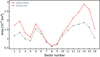 |
Fig. A.3. Dimming area on the plane (dashed black curve) and over the surface (red curve) calculated for each sector. |
We propose the adoption of this approach for a precise correction of all on-disk pixels. In particular, it will be useful for the pixels located close to the limb (beyond 60°), which are disregarded in the classical correction method using a factor of 1/cos α (Hagenaar 2001). By implementing this alternative method, we can achieve enhanced accuracy in the correction process for solar images.
All Figures
|
Fig. 1. Snapshots of coronagraphic observations using JHelioviewer (Müller et al. 2017). Left column: SOHO/LASCO C2 white-light base difference images. Right column: white-light base difference images from STEREO-A COR1. Yellow arrows indicate the CME and red arrows show the propagated leg of the filament eruption at time steps 16:36 UT and 17:36 UT, respectively. |
| In the text | |
|
Fig. 2. View of the ecliptic plane showing the various spacecraft positions on 28 October 2021. SDO is located along the Sun–Earth line, while the STEREO-A and Solar Orbiter spacecraft are positioned 37.6° and 2.8° to the east, respectively. The image was generated using the Solar-MACH tool (Gieseler et al. 2023). |
| In the text | |
|
Fig. 3. Overview of the 28 October 2021 event, showing the dimming evolution and eruption of the filament in AIA 193 Å. Left: direct images. Right: corresponding base-difference images. Four time steps are shown, while the full evolution of the event can be found in the online movie. |
| In the text | |
|
Fig. 4. STIX images showing 50%, 70%, and 90% contours for energy bands 4−10 keV (red), 15−25 keV (blue), and 25−50 keV (dark blue). The STIX contours are rotated to the point of view of SDO and overlaid on AIA images. The AIA images are shown for two different time steps: top row – 15:25 UT, and bottom row – 15:26 UT; and at two different AIA filters: left column – 171 Å, and right column – 1600 Å. |
| In the text | |
|
Fig. 5. Total area of the dimming region. Left: base-difference map at the time of maximal dimming extent at 15:57 UT. Middle: cumulative timing map of the whole dimming extraction, color-coded in minutes from 15:05 UT. Right: same dimming map, but each pixel shows the ratio of its area to the area of the average pixel in the center. Dashed curves and numbers represent the chosen sectors. |
| In the text | |
|
Fig. 6. Dimming area calculated for each sector in the full cumulative map. The shaded band indicates the error estimation using different threshold levels used for the dimming segmentation. The largest dimming area is in sector no. 14. |
| In the text | |
|
Fig. 7. Evolution of the erupting filament between 15:12 and 15:32 UT in SDO AIA 193 Å (top) and STEREO-A EUVI 195 Å direct images (a) and between 15:35 and 15:50 UT in base difference images (b). Blue markers show the upper tip of the filament observed by SDO AIA, and red markers indicate the matching points from the STEREO-A vantage point. Epipolar lines are shown in white. The yellow arrows indicate another, central part of the filament eruption. We note that the image scale of panels a and b is different. An animation of the reconstructions of panel b can be found in the online movie. |
| In the text | |
|
Fig. 8. Connection of the low coronal signatures with the CME propagation further out. Left panels: SDO AIA 193 Å and STEREO-A EUVI 195 Å base-difference images with reconstructed matching points of the eruptive filament (blue and red, respectively) and their orthogonal projections on the surface (green and yellow). The sector with the largest area of dimming is marked by its number (no. 14). Right panels: propagation of the CME seen from SOHO/LASCO C2 (top) and STEREO-A COR2 (bottom) coronagraphs at later time steps. Red arrows indicate the filament development as the bright substructure of the CME. Coronagraphic observations were obtained using JHelioviewer (Müller et al. 2017). |
| In the text | |
|
Fig. 9. Three-dimensional model of the Sun with the reconstructed filament. Red points show the reconstructed heights of the filament. The dark red line shows a linear fit and the red dashed lines represent projections onto equatorial (green) and meridional (red) planes. The black line indicates the radial direction, and the dashed black line shows its projection onto the equatorial plane. Equatorial and meridional planes both go through the intersection of the linear fit with the solar surface (filament origin). The radial direction is located in the meridional plane by definition. For clarity, the heliocentric coordinates grid is shown in gray. The inclination angle from the radial in the equatorial plane is shown as a yellow arc, and the inclination angle in the meridional plane is shown as two red arcs, respectively. |
| In the text | |
|
Fig. 10. Kinematics of the erupting filament and associated SXR flare evolution. (a) Height estimations of the filament (black markers). The error bar presents the five-pixel shift in finding the matching point along the epipolar line. The corresponding black solid line indicates the smoothed height-time profile. (b) Speed and (c) acceleration of the filament obtained by numerical differentiation of height-time data (dots) and smoothed profiles (lines). The shaded areas give the error ranges. (d) GOES 1−8 Å SXR light curve (black curve, left Y-axis) and the corresponding change rate (gray curve, right Y-axis). (e) STIX count rates at 4−10 keV (red), 15−25 keV (blue), and 25−50 keV (dark blue) energies. The vertical dashed lines mark the peaks in the 25−50 keV STIX curve (dark blue), the GOES SXR flux (black), and its derivative (gray). |
| In the text | |
|
Fig. 11. Observations of the CME by SOHO/LASCO C2 (left) and STEREO-A COR2 (right) coronagraphs with the GCS reconstructions (green mesh). |
| In the text | |
|
Fig. 12. Three-dimensional model of the Sun with the GCS croissant (green mesh with blue inner part) and coronal dimming (blue contour). |
| In the text | |
|
Fig. 13. AIA 193 Å base difference image showing the dimming region (blue contour) with an overlaid orthogonal projection of the inner part of the GCS bubble (green mesh). The green marker indicates the source location derived from the GCS reconstruction, and the red marker represents the center of mass of the dimming region. The red mesh illustrates the orthogonal projection of the inner part of the GCS reconstruction, with the source point shifted to the location of the center of mass. |
| In the text | |
|
Fig. 14. Comparison of the two versions of the GCS reconstruction on the SOHO/LASCO C2 16:12 UT image of the CME. The green mesh represents the GCS reconstruction from coronagraph observations, and the red mesh represents the same croissant with a changed location of source chosen by the dimming center of mass. |
| In the text | |
|
Fig. 15. Three-dimensional model of the Sun observed from SDO (left) and STEREO-A (right). The dimming borders are shown with blue contours and the sectors are drawn as light blue lines (the filled area indicates the sector of dominant dimming propagation). Red points mark the reconstructed filament heights, and purple points are their orthogonal projections on the surface. The inner part of the GCS reconstruction is plotted as blue mesh. The dark red line presents the straight line fit to the reconstructed filament positions. The green line shows the axis of the CME, which is represented by the GCS croissant. |
| In the text | |
|
Fig. A.1. Scheme of a solar image. The outer square shows the boundaries of a solar image from a spacecraft. The marker C at the top left corner indicates the pixel with the coordinates (1,1), i - row number, j - column number. The marker C’ also shows the pixel with the coordinates (1,1), but in a new coordinate system with rows i′ and columns j′ connected to i and j via Equation (A.6). “Top”/“Left” show the distance (in pixels) from the top/left border of the image to the beginning of the Sun. P is a pixel, and |
| In the text | |
|
Fig. A.2. Correction area map for the full solar disk at the currently observed radius of the Sun. The colorbar shows the ratio of every pixel area to the average pixel and increases closer to the limb. |
| In the text | |
|
Fig. A.3. Dimming area on the plane (dashed black curve) and over the surface (red curve) calculated for each sector. |
| In the text | |
Current usage metrics show cumulative count of Article Views (full-text article views including HTML views, PDF and ePub downloads, according to the available data) and Abstracts Views on Vision4Press platform.
Data correspond to usage on the plateform after 2015. The current usage metrics is available 48-96 hours after online publication and is updated daily on week days.
Initial download of the metrics may take a while.