| Issue |
A&A
Volume 678, October 2023
|
|
|---|---|---|
| Article Number | A12 | |
| Number of page(s) | 22 | |
| Section | Cosmology (including clusters of galaxies) | |
| DOI | https://doi.org/10.1051/0004-6361/202347000 | |
| Published online | 28 September 2023 | |
The Ie-Re plane and the 3D-kappa space of stellar systems
Diagnostic tools for investigating past evolution
Department of Physics and Astronomy, University of Padova, Vicolo Osservatorio 3, Padova 35122, Italy
e-mail: This email address is being protected from spambots. You need JavaScript enabled to view it.
; This email address is being protected from spambots. You need JavaScript enabled to view it.
; This email address is being protected from spambots. You need JavaScript enabled to view it.
Received:
25
May
2023
Accepted:
14
July
2023
Abstract
Contact. This paper is the fourth in a series dedicated to the observed parallelism of properties passing from globular clusters to early-type galaxies. To a lesser extent, it also covers galaxy clusters and groups.
Aims. Here, we investigate the Ie-Re plane and the 3D-kappa space defined by Bender, Burstein and Faber, as potential diagnostic tools in studies of the past evolution of these stellar systems. In the space of the parameters characterizing a stellar system such as the luminosity, L, stellar mass, Ms, half-light (mass) radius, Re, central velocity dispersion, σc, surface brightness, Ie, and so on, the Ie-Re plane is one of possible projections that was thoroughly investigated over the years with many important results. The 3D-kappa space relies on three variables that are suitable combinations of the logarithms of the above parameters. Among others, perhaps the most important result from this new space is the discovery of the fundamental plane of early type galaxies. In this paper, we intend to explore in more detail the potential capability of the joined investigation of the Ie-Re plane and 3D-kappa space.
Methods. Based on the collected literature data on the mass, half-mass (light) radius, velocity dispersion, and surface brightness in different bands for the objects under investigation, we set up the Ie-Re plane and the 3D-kappa space. We then compared the observed distributions of these objects with those predicted by simple theoretical galaxy models.
Results. We explored the effects of different mass-radius relationships, star formation, infall, and mass assembling histories on the diagnostic planes under examination. We also investigated variations in the 3D-kappa space as a function of the redshift.
Conclusions. We show that the distribution of the stellar systems on the various diagnostic planes can cast light on the mass-radius relation and the history of star formation in stellar systems going from globular clusters to early type galaxies.
Key words: Galaxy: fundamental parameters / Galaxy: formation / galaxies: evolution / galaxies: stellar content / galaxies: high-redshift / globular clusters: general
© The Authors 2023
 Open Access article, published by EDP Sciences, under the terms of the Creative Commons Attribution License (https://creativecommons.org/licenses/by/4.0), which permits unrestricted use, distribution, and reproduction in any medium, provided the original work is properly cited.
This article is published in open access under the Subscribe to Open model. This email address is being protected from spambots. You need JavaScript enabled to view it. to support open access publication.
1. Introduction
This paper is a sequel of a series dedicated to the observed parallelism of properties across globular clusters (GCs) and early-type galaxies (ETGs) to galaxy clusters and groups (GCGs; D’Onofrio et al. 2019; D’Onofrio et al. 2020; Chiosi et al. 2020). It is widely known that in the space of specific intensity, Ie (and companion luminosity L), half-light (-mass) radius, Re, central velocity dispersion, σ, and mass in stars, Ms, it is possible to set up sub-spaces and projection planes in which useful relations are found. Each of these relations yields some partial information: for instance, the fundamental plane (FP) of galaxies (Dressler et al. 1987; Faber et al. 1987; Djorgovski & Davis 1987), L-σ relation (Faber & Jackson 1976), mass-radius relation (Chiosi et al. 2020), and, finally, the so-called 3D kappa space (3DKS; Bender et al. 1992; Burstein et al. 1997), which we briefly define below.
The aim of this study is to show that a simultaneous analysis of the distribution of these objects in the Ie-Re plane and in 3DKS can provide useful information on the past history of mass aggregation and star formation, as well as the underlying mass-radius relationship (MRR).
The analysis was based on the observed distribution of stellar aggregates from globular clusters to giant ellipticals (and also to galaxy clusters) in the Ie-Re plane and the 3DKS. The specific intensity Ie and luminosity L refer to a certain band in use (typically B and/or V, unless otherwise specified). For the aims of our study, first we set up a simple model simulating the astrophysical objects of different mass under investigation by means of the mean single stellar population (SSP) approximation. Second we made use of the N-Body hydrodynamic simulations of galaxies taken from different sources, namely, the Illustris models of Vogelsberger et al. (2014a,b), Genel et al. (2014), Nelson et al. (2015; to whom we refer for all details) in the fully hierarchical scheme), of Chiosi & Carraro (2002; in the monolithic scheme) and of Merlin et al. (2010, 2012; in the early hierarchical scheme), and finally the semi-analytical infall models originally proposed by Chiosi (1980) and subsequently developed by Tantalo et al. (1998). The goal was to infer the past duration of the star formation activity, the underlying MRR, the FP in its most popular projection, that is, when seen edge-on, the boundary line for the so-called zone of exclusion (ZOE) in the Ie-Re plane, the distribution in the 3DKS, and, finally, the possible variation of these relationships with the redshift.
The plan of the paper is as follows. In Sect. 2, we briefly recall the definition of the 3DKS. In Sect. 3, we present the observational data we used in our analysis and the numerical hydrodynamic models of galaxy formation and evolution we adopted. In Sect. 4, we outline the strategy of the analysis based on three steps of increasing complexity. In Sect. 5, we present simple galaxy models based on the concept of single stellar populations (SSPs) for objects of different mass, mass-radius relation (MRR), and star formation history (SFH). In Sect. 6, we present the results obtained with the simple SSP-model (first step). In particular, we discuss the location of the models on the Ie-Re plane and 3DKS at the present time. The results are discussed in some detail at varying the MRR and the ratio of dark mass, MDM, to stellar mass, Ms. Finally, we present the reference case. In addition to this, we derive the border line separating in each plane (Ie-Re and projection planes of the 3DKS) the permitted area, where all stellar complexes of any mass should be found, from the forbidden one, where no object can exist. The concept of zone of exclusion (ZOE), introduced by Bender et al. (1992) is extended to encompass the new results. We also discuss the relationships among MRR, the ZOE-border and the fundamental plane. In Sect. 7, we present the results obtained from infall galaxy models of Chiosi (1980) and Tantalo et al. (1998) that should supersede the SSP-models (second step) showing that excellent agreement can be achieved also in this case. In Sect. 8, we make use of detailed hydrodynamic galaxy models (mainly Illustris) and perform the third step of the analysis showing how the various diagnostic planes (Ie-Re and those of the 3DKS) change with the redshift, arguing that the fundamental plane and MRR for ETGs share the same origin and formation time. In Sect. 9, we discuss the fundamental plane for ETGs in more detail using different photometric systems and detailed NB-TSPH1 model galaxies. Some conclusions are drawn in Sect. 10. Finally, in Appendix A, we briefly present two analytical SSP-models that are based on MRRs that did not give satisfactory results.
For the sake of internal consistency with the previous studies of the series, in our calculations, we assumed the same values of the Λ-CDM cosmology used in the Illustris simulations by Vogelsberger et al. (2014a),b): Ωm = 0.2726, ΩΛ = 0.7274, Ωb = 0.0456, σ8 = 0.809, ns = 0.963, and H0 = 70.4 km s−1 Mpc−1.
2. Definition of the kappa space
The 3DKS was first introduced by Bender et al. (1992). They started from the studies of dynamically hot galaxies by Dressler et al. (1987), Faber et al. (1987), and Djorgovski & Davis (1987) who showed that these objects lie on a plane (i.e., the fundamental plane) in the 3D space defined by log σc, log Ie, and log Re, where σc is the central velocity dispersion, Ie the mean surface brightness, and Re the half-light (mass) radius of the luminous part of a galaxy.
The three quantities are related to each other by:
 (1)
(1)
 (2)
(2)
 (3)
(3)
where L and M are the luminosity and the mass (in solar units), and
 (4)
(4)
 (5)
(5)
with G as the gravitational constant and Kv as a form factor that (in principle) can vary from galaxy to galaxy (it measures the degree of anisotropy in the velocity field of a galaxy; see Bender et al. 1992, for more details on this topic).
Bender et al. (1992) translated the physical coordinates to new coordinates (on logarithmic scale) by means of the following relations:
![Mathematical equation: $$ \begin{aligned}&k_1 \propto \log \left[ \frac{ M }{c_2} \right] ,\end{aligned} $$](/articles/aa/full_html/2023/10/aa47000-23/aa47000-23-eq6.gif) (6)
(6)
![Mathematical equation: $$ \begin{aligned}&k_2 \propto \log \left[ \frac{c_1}{ c_2} \left(\frac{M}{ L }\right) I_{\rm e}^3\right] ,\end{aligned} $$](/articles/aa/full_html/2023/10/aa47000-23/aa47000-23-eq7.gif) (7)
(7)
![Mathematical equation: $$ \begin{aligned}&k_3 \propto \log \left[{ \frac{c_1 }{c_2 }} \left( \frac{M}{L }\right)\right]. \end{aligned} $$](/articles/aa/full_html/2023/10/aa47000-23/aa47000-23-eq8.gif) (8)
(8)
Owing to the definition of the surface brightness, c1 is a numerical constant that can be included in the derivation of Ie itself. As pointed out by Bender et al. (1992) if the mass-to-light ratio is a weak function of L ((M/L)∝L0.2 ) and c2 is a constant for all galaxies, the equation for the FP is easily derived from Eq. (3). Starting from this, Bender et al. (1992) formulated the equations transforming the space σ, Re, and Ie into the space k1, k2, and k3, and applied a suitable rotation to obtain an orthogonal coordinate transformation. The final set of equations, where c2 ≡ 1/Kv is left in evidence, is as follows:
 (9)
(9)
 (10)
(10)
 (11)
(11)
The projection of the FP onto the k1 − k3 plane is the FP seen edge-on. Using the elliptical galaxies of the Virgo to avoid distance uncertainties, the relation k3 = 0.15k1 + 0.36 with σ(k3) = 0.05 was found (cf. Ciotti et al. 1996, for details). The ratio (M/L) seems to increase with galaxy mass (tilt of the FP).
3. Observational data and theoretical models
In this section, we introduce both the observational data for globular clusters, galaxies of different mass, and galaxy clusters and groups, and the theoretical numerical simulations of galaxies and galaxy clusters used in this study.
Observational data. The observational data are: (i) The catalog of ETGs, late-type galaxies (LTGs), dwarf galaxies (DGs), GCs, and GCGs in the Local Group and Local Universe by Burstein et al. (1997). Over the years, this very popular sample has been examined by many authors so that a detailed presentation is superfluous here. It is worth recalling that the masses assigned to DGs by Burstein et al. (1997) are the dynamical masses and not the stellar masses, so this group is not strictly homogeneous with the sample for ETGs. The 3DKS of these objects is for the luminosity and surface brightness in the B-band. Finally, the list of DGs for the local Group is supplemented by that of Woo et al. (2008), Geha et al. (2006), Hamraz et al. (2019), and that of galactic GCs of Burstein et al. (1997) by the data of Pasquato & Bertin (2008) and the transition objects from GCs to DGs of Kissler-Patig et al. (2006). (ii) The much richer sample of SDSS data for ETGs by Bernardi et al. (2010) roughly covering the redshift interval z = 0 to z ≃ 0.27. The sample contains ≃60 000 galaxies of which we used only those with redshift smaller than z = 0.1. The ETGs of this sample fully overlap those ETGs of Burstein et al. (1997). (iii) The samples of ETGs, bright central galaxies (BCGs) and GCGs set up by Valentinuzzi et al. (2011), Cariddi et al. (2018) using the data of the WIde-field Nearby Galaxy-cluster Survey (WINGS) of Fasano et al. (2006) and Varela et al. (2009) and companion OMEGA-WINGS extension of Gullieuszik et al. (2015) and Moretti et al. (2014, 2017) for a number of clusters in the redshift interval (0.04 ≤ z ≤ 0.07).
General remarks. For the sake of illustration we show in Fig. 1 the 3DKS of the observational data limited to the Burstein et al. (1997) sample, using different colors for the different objects of the list as indicated. The ETGs of Bernardi et al. (2010) overlap those of Burstein et al. (1997). The same happens for the WINGS objects. The most important thing to note is that the three groups agree with each other. Furthermore, it is important to remember here that these heterogeneous data samples are not statistically complete. They are used here only to show, in a qualitative sense, the distribution of the different astrophysical objects under consideration in our diagnostic planes. Information and details on how the stellar masses, Ms, half-mass radii, Re, specific intensity, Ie, and velocity dispersion, σ, have been derived can be found in the original sources to which the reader should refer. Of course some possible systematic biases among the different sets of data are expected, whose entity ought to be small. However, since the groups of objects will be treated separately and only from a general qualitative point of view, no homogenization of the data is needed. Furthermore, apart from the different richness of the three samples, we can say that there is no substantial difference passing from one sample to another.
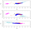 |
Fig. 1. 3DKS of the Burstein et al. (1997) data and the Illustris sample. The red dots are the ETGs, the green dots the LTGs, the coral dots the DGs, the magenta dots the GCs, the light-blue dots the GCGs, and the blue dots are the Illustris galaxies. To avoid overcrowding of the panels that data of Bernardi et al. (2010) and of the WINGS survey are not plotted. They overlap the Burstein et al. (1997) data. However, it is worth recalling that the observational data of Burstein et al. (1997) are in the B-band while the Illustris models are in the V-band. Consequently, there is a systematic offset among the two groups of data. Therefore, the comparison is only of qualitative nature. Nevertheless, the Illustris models overlap the LTGs, ETGs and a large part of the DGs, implying an acceptable agreement between theory and observations. |
Theoretical models. We briefly present the numerical simulations of galaxies and clusters that we used to interpret and reproduce the properties of their observational counterparts. They are ordered in terms of complexity and available information.
The pure monolithic scheme. Chiosi & Carraro (2002), by means of hydrodynamic simulations, incorporating radiative cooling, star formation, energy feedback, and chemical evolution, addressed the problem of the formation and evolution of ETGs (from dwarf to normal and giant systems) in the framework of the SCDM cosmological model of the Universe and monolithic scheme of galaxy formation. The cosmological parameters are H0 = 65 km s−1 Mpc−1, baryonic-to-dark-matter ratio, MBM/MDM, is equal 1 to 9, that is, for MT = MBM + MDM, MBM = 0.1MT, MDM = 0.9MT (with obvious meaning of symbols), and the redshift at which galaxies were supposed to start the collapse (zf ≃ 1 and zf ≃ 5). The key results of this study are: (i) the duration, strength and shape of the star formation rate as function of time strongly depend on the galaxy mass and the initial density; (i.a) galaxies of a high initial density and total mass over a wide range undergo a prominent initial episode of star formation, then followed by quiescence; (i.b) the same applies to high-mass galaxies of low initial density, whereas the low mass ones undergo a series of burst-like episodes that may stretch up to the present. The details of their star formation history (SFH) are also very sensitive to the value of the initial density; (ii) the mass turned into stars per unit total mass of the galaxy is nearly constant, which means that the engine at work is the same; (iii) the ratio between the left-over gas to the initial total baryonic mass decreases at increasing total mass of the galaxy; (iv) as a result of star formation in the central core of the galaxy and consequent gas heating, large amounts of gas are pushed to large distances. After cooling, part of the gas falls back towards the central furnace; (v) galactic winds are at work. In general, all galaxies are able to eject part of their gas content into the inter-galactic medium. However, the percentage of the ejected material increases at decreasing galaxy mass. All other details of these models can be found in Chiosi & Carraro (2002).
The early hierarchical scheme. With the aid of the parallel hydrodynamic code EvoL, Merlin et al. (2010, 2012) produced a number of models for ETGs with different mass and/or initial density (twelve cases in total). The models were followed from the epoch of their detachment from the linear regime, that is, zi ≥ 20, to a final epoch (redshift, zf) different from model to model (however, with zf ≤ 1). The simulations included radiative cooling down to 10 K, star formation, stellar energy feedback, re-ionizing photo-heating background, and chemical enrichment of the interstellar medium. The reader can refer to the cited papers for all the details on the code and results. The assumed cosmology was the standard Λ−CDM, with H0 = 70.1 km s−1 Mpc−1, flat geometry, ΩΛ = 0.721, σ8 = 0.817; the baryonic fraction ≃0.1656. In general, the collapse occurred during the redshift interval 4 > z > 2, it started first in the central regions and gradually moved outwards. The collapse was complete at redshift z ≃ 2. All the models developed a central stellar system, with a spheroidal shape. Massive halos (MT ≃ 1013 M⊙) experienced a single, intense burst of star formation (with rates ≥103 M⊙/yr) at early epochs, consistently with the observations, with a less pronounced dependence on the initial density; intermediate mass halos (MT ≃ 1011 M⊙) had star formation histories that strongly depend on their initial density, that is, from a single peaked to a long lasting period of activity with strong fluctuations in the rate; finally, small mass halos (MT ≃ 109 M⊙) always had dscontinuous star formation histories, resulting in multiple stellar populations, due to the so-called “galactic breathing” phenomenon. They confirmed the correlation between the initial properties of the proto-halos and their star formation histories already found by Chiosi & Carraro (2002). The models had morphological, structural, and photometric properties comparable to those of real galaxies, closely matching the observed data (see Merlin et al. 2012, for all other details) overall. These models were classified as “early hierarchical” because they underwent repeated episodes of mass accretion of sub-lumps of matter inside the original density contrast in very early epochs and essentially evolved in isolation ever since.
The fully hierarchical view. Our primary source of data is the Illustris compilation2 (Vogelsberger et al. 2014a,b; Genel et al. 2014; Nelson et al. 2015, for all details), a suite of large, highly detailed cosmological hydrodynamic simulations, including star, galaxy and black-hole formation, along with tracking the expansion of the universe (Hinshaw et al. 2013). The procedure we adopted to extract theoretical data from the Illustris database is broadly described in D’Onofrio et al. (2020). We just mention here that for each galaxy of the samples at different redshifts (i.e., z = 4, z = 3, z = 2.2, z = 1.6, z = 1, z = 0.6, z = 0.2, and z = 0), we extracted the stellar mass, Ms, the dark matter mass, MDM, the total baryonic mass, MBM(inclusive of gas), the luminosity (magnitude) in the V band, the half-mass radius of the stellar component, Re, and of the dark component, RDM, the velocity dispersion σs and σDM, and, finally, the star formation rate (SFR). Care was taken to trace back each object present in the list at z = 0 throughout the previous epochs according to the identification codes provided by the Illustris Team. In this way, the past evolutionary history of each object could be followed in detail. At the beginning the ratio ω = MDM/MBM is fixed by the cosmological model of the Universe, in our case for Ωm/Ωb = 0.2726/0.0456, we get ω = 5.92 ≃ 6. It is worth keeping in mind that over the course of the formation and evolution processes, the above masses can change in presence of galactic winds and/or stripping and/or acquisition of material by interactions with other galaxies or intergalactic medium.
It is mandatory to recall here that the Illustris-1 suite of galaxy models was superseded by Illustris-TNG of Springel et al. (2018), Nelson et al. (2018), and Pillepich et al. (2018), and EAGLE by Schaye et al. (2015). We decided to adopt here Illustris-1 for two reasons: firstly, the fact that we wanted to be consistent with the results shown in our previous papers on this same subject that were based on the Illustris-1 models; secondly, we checked that the main results of our analysis do not change passing from Illustris-1 to Illustris-TNG (see for instance D’Onofrio & Chiosi 2023a; D’Onofrio & Chiosi 2023b). The kind of analysis carried out here is indeed somehow independent of the level of precision reached by models from different sources, because we were mainly interested in presenting a new method to decrypt the information enclose in the observational data about the past history of ETGs.
General remarks. The fully hierarchical scheme is the most difficult case to deal with because of the frequent mergers among galaxies of different mass, size, and age. If gas is present, recurrent episodes of strong star formation activity may occur. It is conceivable that seed galaxies prior to any encounter behave like the first two schemes envisaged before and are governed by the initial density and mass. Mergers among objects of similar mass would likely enhance the rate of star formation in a sort of burst of short duration and then fold the two histories together. Mergers among objects of much different mass, would simply generate a temporary perturbation on the star formation history of the most massive one, while less massive object simply loses its identity.
In addition, we recall that the three groups of theoretical models we have used differ in many details of their input physics, such as energy injections, cooling processes, chemical enrichment prescriptions, computational technicalities, and so forth. Nevertheless, the fact that they crowd the same regions in various diagnostic planes, such as the MR plane, the Ie-Re plane, and the 3DKS projection planes, strongly suggests that at the end, they are all equivalent in the sense that they all agree in reproducing the main properties of the astrophysical objects they refer to.
For the sake of illustration we show in Fig. 1 the 3DKS for model galaxies of the Illustris sample at redshift z = 0. They essentially overlap the region occupied by ETGs and bright DGs of the Burstein et al. (1997), Bernardi et al. (2010), and WINGS objects (these latter two are not plotted to avaid overcrowding of panels). The comparison is however merely qualitative because magnitudes, luminosities, and surface brightness of the four groups are not the same: the Bernardi et al. (2010) data are in V-band, the WINGs data are in B and V-bands, the Burstein et al. (1997) data are in the B-band, and, finally, Illustris models are only in the V-band. Therefore, a systematic small shift between the galaxies of Illustris and those of the other three groups exists, but fortunately it does not significantly affect our discussion.
4. Strategy of the analysis
In this section, we briefly sketch out the strategy of this study, which proceeds in steps of increasing complexity. Firstly, we proposed a simple analytical model of galaxies, based on the concept of single stellar population that is meant to highlight the main physical causes of the distribution of stellar assemblies from GCs and DGs to LTGs, ETGs, and (possibly) GCGs in the 3DKS and its projection planes k2 vs. k1, k3 vs. k1, and k2 vs. k3. Secondly, we strengthened the results of the simple analysis by means of the so-called infall models adapted to the present scientific cases. Thirdly, we addressed to current NB-TSPH galaxy models in literature and repeated the analysis largely confirming the results obtained in the previous steps but now framing them in more physically consistent contexts. Particular attention was paid to interpret the fundamental plane and to highlight the evolution of the 3DKS with time and redshift. Finally, we discussed the (Ms/Ls)−Ms plane and the fundamental plane with the aid of detailed NB-TSPH galaxy models. In more detail, the four steps are:
Analytical model. Galaxies of given stellar mass, Ms, luminosity, Ls, and radius, Re, were reduced to SSPs of the same stellar mass, luminosity, and radius; to this aim, a suitable Re vs. Ms relationship is required to get the velocity dispersion σ and another one between Ls, Ms, and the mean duration of the star formation activity to obtain a plausible estimate of the galaxy surface brightness, Ie.
Infall models. The galaxy models developed by Tantalo et al. (1998) were adapted to the present case and were used to follow the growth of the stellar content by infall of gas coupled to star formation and chemical enrichment. At each time, the current stellar content was used to estimate an effective radius by means of a mass-radius relationship taken from literature (Chiosi et al. 2020). Finally, the star formation history was used to derive the evolution of luminosity. This allowed us to know the evolution on the Ie-Re plane and of the projection planes of the 3DKS of galaxies with different mass.
NB-TSPH models. Using the Illustris hierarchical simulations we repeated the analysis and derived the 3DKS for galaxies with minimum mass in the range 106–109 M⊙ and maximum mass of about 1013 M⊙. The Illustris models were extensively compared with data and the theoretical results of the analytical and infall models throughout steps one and two, while in step three, they were used to investigate the time and redshift evolution of the 3DKS and the Ie-Re plane.
Detailed NB-TSPH models. Finally, with the aid of the two small groups of model galaxies calculated in the monolithic scheme (Chiosi & Carraro 2002) and the early hierarchical scheme (Merlin & Chiosi 2006, 2007; Merlin et al. 2010, 2012; Chiosi et al. 2014; Chiosi & Merlin 2015), we recalculated the parameters of the 3DKS at z = 0 (present time), using the integrated photometry technique based on the star by star luminosities and colors and compared the results with data for the local Universe to further validate the results obtained with the point mass photometry.
5. Outline of the analytical model
The complexity of real globular clusters, galaxies and galaxy clusters was reduced to ideal SSPs of given total stellar mass, Ms, and half-mass (half-light) radius, Re, and embedded in an environment of dark matter (DM) with mass, MDM, with radius, RDM. This ideal SSP has mean metallicity, Z, and an age, Tstars, which is also the age of the stellar content. The total stellar mass is related to the mean star formation rate, ⟨Ψ⟩, by the relation, Ms = ⟨Ψ⟩Tstars. The model set up is as follows:
Firstly, we started from the relationship linking the halo mass, MDM, the stellar mass, Ms, and the radius, Re, in ideal objects of different mass spanning the range from from GCs to GCGs.
Secondly, we estimated the stellar velocity dispersion by means of the virial theorem. At each time, an object is supposed to be in condition of mechanical equilibrium, hence satisfying the following relation:
 (12)
(12)
Thirdly, to the mass, Ms, we assigned a typical mean value of the age of the bulk stellar content and derived the present day luminosity, LΔλ, of the object in the band, Δλ, of interest. Knowing Ms and Re, we could calculate the surface brightness, and, finally, the coordinates k1, k2, and k3 of the 3DKS.
5.1. The Re(Ms) and the Ms(MDM) relationships
Basic ingredients of the models are: (a) the Ms-Re relation that in turn requires two more relationships, namely, MDM-Ms and MDM-Re. The first one is the mass in stars built up in a galaxy of total mass of dark matter, MDM, over the course of its lifetime and measured at the present time. Usually this is expressed by the ratio, MDM/Ms, as a function of MDM. (b) The luminosity LΔλ or the magnitude MΔλ vs. age relationships for SSPs, where Δλ is some pass-band depending on the observational data to disposal.
The mass-radius relationship (MRR) was thoroughly investigated by Chiosi et al. (2020) to which the reader should refer for all details. We recall here the three MRRs derived by the authors that are also used here:
Observational MRR (i). Taking the sample of ETGs by Bernardi et al. (2010) as the reference case because of its richness, the MRR is then:
 (13)
(13)
where Ms is in M⊙ and Re in kpc. Similar relations (with nearly the same slope and zero-points) can be derived using the data for ETGs by Burstein et al. (1997) and Valentinuzzi et al. (2010). Extrapolating these relations downward to the mass range of GCs and upward to that of GCGs, they would provide a lower limit to GCs, pass through dwarf ellipticals like ωCen and M32, yield the lowest limit to the distribution of DGs, and finally, hit the region of GCGs.
Dwarf galaxies seem to obey a different relation. Taking the richest sample for this group (Woo et al. 2008) the best fit yields:
 (14)
(14)
with slope that is about half of the one for ETGs. Masses and radii are in solar units and kpc, respectively. Table 1 lists the MRRs derived from observational data for ETGs and DGs that are used in this study.
MRRs derived from observational data and expressed as log Re = Alog Ms + B adopted in this study.
The MRR of collapsing DM proto-halos (ii). In the context of the Λ-CDM cosmology, Fan et al. (2010) derived an expression linking together (a) the halo mass MDM, (b) the stellar mass Ms of the galaxy born inside it, (c) the half light (mass) radius Re of the stellar component, (d) the redshift at which the collapse took place zf, (e) the shape of the baryonic component of a galaxy (via the coefficient SS(nS) related to the Sersic brightness profile from which the half-light radius is inferred and the Sersic index nS), and (f) the velocity dispersion of the baryonic component with respect to that of dark matter expressed by the parameter fσ, that is, σs = fσσDM, and, finally, (g) the ratio m = MDM/Ms. The expression for the MRR is:
 (15)
(15)
where, following Fan et al. (2010), we adopted SS(nS) = 0.34 and fσ = 1. For more details see Fan et al. (2010) and references therein. The most important parameter of Eq. (15) is the ratio m = MDM/Ms that is briefly discussed below. The MRR of Eq. (15) is the locus on the MR plane of galaxy models, the formation of which began at a redshift zf. The slope of this relation is about half of that for ETGs and much akin to that of DGs. This MRR can be safely used in the monolithic scenario, while in the hierarchical case, it provides only a qualitative hint.
The MRR Cosmic Galaxy Shepherd (iii). The observed distribution of astrophysical objects on the MR plane, going from GCs to galaxies of different mass and morphological type and eventually to GCGs, strongly suggested that a unique relation could exist for all of them and that such a relation likely owes its origin to the cosmological growth of DM halos. More details can be found in Chiosi et al. (2020).
The distribution of the DM halos and their number density as a function of redshift was the target of the large scale numerical simulations of the Universe. We refer to the Millennium Simulation of Springel et al. (2005), the Illustris Simulations of Vogelsberger et al. (2014a),b), Genel et al. (2014), Nelson et al. (2015), and the Illustris-TNG Simulations of Pillepich et al. (2018), and Nelson et al. (2019), and references there in. In parallel, analytical studies of the “halo growth function (HGF)” as the integral of the “halo mass function (HMF)” appeared in literature (see, e.g., Lukić et al. 2007; Angulo et al. 2012; Behroozi et al. 2013). In brief, the HGF gives the number density of halos of different mass per (Mpc/h)3 emerging at each epoch by all creation and destruction events and consequently yields the halos that nowadays populate the MR plane and generate the observed galaxies. Chiosi et al. (2020) adopted the HGF of Lukić et al. (2007) who, using the ΛCDM cosmological model and the HMF of Warren et al. (2006), derived the number density of halos n(MDM, z) over ample intervals of halo masses and redshifts. Since n(MDM, z) of Lukić et al. (2007) refers to a volume of 1 (Mpc/h)3, before being compared with the observational data it must be scaled by a suitable factor in order to match the volume sampled by observations. Assuming a certain number density of halos, Ns, derived from the observational data, Chiosi et al. (2020) set up the equation n(MDM, z) = Ns whose solution yields the mass of the typical halos, MDM(z), as a function of the redshift and vice-versa the redshift for each halo mass. To each value of MDM from this function one can associate a pair of Ms and Re. For Ns = 10−2 halos per (Mpc/h)3 – roughly the volume surveyed by the SDSS (see Chiosi et al. 2020, for details) – the resulting curve, Re(Ms), falls at the edge of the observed distribution of ETGs in the MR plane. Higher Ns would shift the curve to larger halos, the opposite for lower Ns. At this point, for each value of the redshift one can draw in the MR plane the locus of the most massive halos given by HGF.
The best fit of this locus and, thus, the extrapolation of it downward to GCs and upward to GCGs is given by the relation:
![Mathematical equation: $$ \begin{aligned} \log R_{\rm e}&= 0.007584 [\log (M_{\rm DM})]^3 - 0.1874\,[\log (M_{\rm DM})]^2 \nonumber \\&\quad + 1.908 [\log (M_{\rm DM})] - 9.027, \end{aligned} $$](/articles/aa/full_html/2023/10/aa47000-23/aa47000-23-eq16.gif) (16)
(16)
where Re and MDM are in the usual units and MDM = Ms × m, for which a mean value of m = 25 was adopted. We note that (a) the locus on the MR plane predicted by Ns = 10−2 halos per (Mpc/h)3 nearly coincides with the observational MRR; (b) the slope of this locus gradually changes from 0.5 to 1 going from low masses to high masses in agreement with the observational data (see van Dokkum et al. 2010, and references therein); (c) along this line the formation redshift gradually decreases from zf ≃ 10 at the bottom left (domain of GCs) to zf ≃ 1 at the top right (domain of bright ETGs; (d) finally, Eq. (16) is ultimately tracing on the MR plane the locus of top end of the halo masses (and their associated baryonic objects) that can exist at each redshift. Chiosi et al. (2020) named this locus the “Cosmic Galaxy Shepherd”.
The Cosmic Galaxy Shepherd gives a profound physical meaning to the line splitting the MR plane into two regions, namely, the region where galaxies are found, from that where no objects are seen. We suggest that Cosmic Galaxy Shepherd is the analog of the edge line defining the zone of avoidance, otherwise known as the zone of exclusion (ZoE) in the 3DKS projection planes, found long ago by Burstein et al. (1997).
The three MRRs under examination are shown in Fig. 2, where they are compared with the observational data in use.
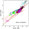 |
Fig. 2. Re-Ms plane of the observational data and theoretical models adopted in this study. Data: here, we show three sources of observational data and two types of MRRs. The samples of data are: (i) Burstein et al. (1997) for GCGs (light powder-blue dots), ETGs (red dots), DGs (blue dots) together with those by Geha et al. (2006) and Woo et al. (2008; green dots), and GCs (violet dots); (ii) The Bernardi et al. (2010) data for ETGs (dark red dots) together with their best fit (the long dashed line). These ETGs fully overlap those of Burstein et al. (1997); (iii) The WINGS data for GCGs (dark grey dots), BCGs (black dots), and ETGs (purple dots). Also in this case there is full coincidence with the corresponding objects of the previous samples. MRRs: the dark goldenrod thick solid line is the Cosmic Galaxy Shepherd of Chiosi et al. (2020) at redshift z = 0; this MRR folds together the galaxy MRR expected from cosmological HDF of halos. The solid orange lines are MRRs of Fan et al. (2010) for redshift zf = 0 (top), 1, and 5 (bottom). Models: theoretical hydrodynamic models of galaxies to be compared with observational data are (i) the Illustris galaxies (light green small dots) for z = 0 that are partially masked by the observational data of ETGs; (ii) the low initial density models (blue filled circles joined by their best-fit line) and the high initial density ones (red filled circled joined by their best-fit) by Chiosi & Carraro (2002); and (iii) the early hierarchical models by Merlin et al. (2012; black squares and their best-fit). See the text for more details. |
TheMDM/Msratio (iv). Based on the Illustris data, Chiosi et al. (2020) investigated how this ratio varies in the mass interval 108.5 < MDM < 1013.5 (masses are in M⊙) and from z = 0 to z = 4. They found that the following relation,
 (17)
(17)
interpolates the Illustris data well. However, they also suggested that for the purposes of simple analyses like the present one, a much simpler relation can be used:
 (18)
(18)
5.2. Duration of star forming activity, luminosity, and surface brightness
The analytical model stands on the concept of single stellar population (SSPs), that is, coeval assemblies of stars with the same chemical composition. Consequently, the stellar content of a galaxy can be considered as a manifold of SSPs of different age and chemical composition, the relative percentage of which in the total mix is determined by the star formation rate as a function of time. Therefore an SSP is the elemental unit of the stellar mix of a galaxy. In an SSP, the percentage of stars of different mass in each mass interval obeys the so-called initial mass function (IMF), ϕ(m) expressed either in mass or in number the integral of which all over the permitted mass interval of real stars yields the total mass of each SSP, that is,  , with a straightforward meaning for the symbols. The IMF is an important ingredient of the SSP theory that deserves some comments. The most popular IMF in literature is due to Salpeter (1955), a simple power law of the mass ∝m−x extending from a lower ml to an higher mass limit, mu. Originally proposed for the stars in the Galactic disk, over the years it has widely used in many other physical contexts. The IMF was long expected to vary with the physical properties of the environment (chemical composition, temperature, density, velocity dispersion of molecular clouds, and son on), or type of environment, that is, star clusters, galaxy type, and so forth. The first studies on an IMF systematical changing with the environment and the galaxy type (mass) from dwarfs to ellipticals were by Padoan et al. (1997), Larson (1998), Chiosi et al. (1998), and Padoan & Nordlund (2002), followed by many others among which we recall Larson (2003) and the recent ones by Dib et al. (2017) and Dib (2022). However, in the present study we simplified all of that and adopted the classical IMF of Salpeter (1955) with slope in number x = −2.35, lower mass ml = 0.1 M⊙, upper mass mu = 100 M⊙, total SSP mass Mssp = 5.82 M⊙, and adopted SSPs with metallicity from Z = 0.0004 to Z = 0.04, six values in total, and age from 10 Myr to 14 Gyrs) of the library set up by Bertelli et al. (2008, 2009), and Tantalo (2005). The absolute MB and MV magnitudes of these SSPs were plotted against the logarithm of the age in years as shown in the panels of Fig. 3. For each band, we also derived the mean age-magnitude relation as shown by the black solid lines with dots in the two panels of Fig. 3. Owing to the nearly linear behavior of each relationship, a linear fit is suited to obtain the relation between the mean absolute magnitude and the logarithm of the age T. These are given by:
 (19)
(19)
 (20)
(20)
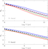 |
Fig. 3. MB (top) and MV (bottom) magnitudes vs. age relationships for SSPs of different metallicities that are indicated by the color code. From the top to the bottom, the metallicies are Z = 0.0001, 0.001, 0.010, 0.019, 0.040, and 0.070. The black dotted lines are the mean values of MB and MV over the metallicity. |
The age is expressed in years. These relationships are an unweighted mean, giving equal weight to all metallicities, and are meant to mimic the mixture of chemical compositions in a galaxy. Although, the distribution of metallicity in the stellar mix of a real galaxy differs from the unweighted mean, our approximation is fully adequate to the aims of this study.
To proceed further, we started from a few considerations suggested by current observational data: (i) GCs, many dwarf elliptical galaxies (DEs) and ETGs are old objects as far as their stellar content is concerned; (ii) the cosmic star formation rate that is found to peak in the redshift interval 1–2 (see the analysis of Chiosi et al. 2017); (iii) the study of the cosmic CMD of galaxies by Sciarratta et al. (2019) indicating that the majority of ETGs are likely made by old stars; and (iv) the results for the star formation history in theoretical model galaxies that is short in massive or high density objects and diluted over long periods of time, often in a series of bursts, in low mass or low density objects as found by Chiosi & Carraro (2002), Merlin & Chiosi (2006, 2007), Merlin et al. (2010, 2012), Chiosi & Merlin (2015), and Chiosi et al. (2014). In setting all these elements together, we propose a simple way of taking all this into account by introducing a relationship between the mean duration of the star formation activity ΔTsfr and the mass of a system. All objects are supposed to initiate their life and star-forming activity in a remote past; however, depending on the mass the duration of star formation was short in GCs and DEs, long in low-mass DGs and intermediate-mass ETGs, and short again in massive ETGs. After trying several analytical expressions, such as Gaussian law or a bi-half-Gaussian with the peaks separated by a linear trend, and others, we found that the following prescription yields good results.
The age of the stars, Tstars, of the last generation in a galaxy is given by:
 (21)
(21)
where TU is the present age of the Universe TU = 13.8 Gyr, and TU(birth) the age of the Universe at the epoch of initial galaxy formation for which we take TU(birth) ≃ 1 Gyr at z ≃ 5. With these assumptions we proposed two linear relations, one for the mass range of GCs and DEs (roughly from 105 to 108 M⊙) and another one for objects in the mass interval 108–1013 M⊙s. We obtained
 (22)
(22)
 (23)
(23)
This age was inserted into Eqs. (19) and (20) to derive:
 (24)
(24)
 (25)
(25)
for objects from GCs to DEs, and then:
 (26)
(26)
 (27)
(27)
for galaxies in the mass range from DGs to ETGs. Estimates of Tstars and ΔTsfr are given in Table 2 for the assumed values of TU and TU(birth). The mass range of application of the two relationships is 5 ≤ log Ms ≤ 8 for GCs and DE galaxies (GLO) and 8 ≤ log Ms ≤ 13 for DG and ETG galaxies.
Estimates of the duration of star formation activity ΔTsfr and age of the last episode of star formation Tstars in objects of different stellar mass Ms.
To summarize, for each stellar mass, Ms, we associated a typical age of the last stellar generation, derived suitable relations between the absolute magnitudes, MV and MB, and the mass, Ms, of the metallicity-averaged SSP representing the galaxy (Eqs. (24) and (26)). We inverted the magnitudes to derive the luminosity in each band, divided by the SSP mass (5.826 M⊙ in our case), then re-scaled the luminosities to the galaxy stellar mass, and, finally, divided the luminosities by  to obtain the surface brightness, Ie, in the B- and V-bands. The whole procedure can be repeated for other bands and photometric systems, as required by the available data. Unless otherwise specified, most of the data in usage here are in the B- and/or V-band of the Johnson system.
The crucial parameter here is the radius Re, which can significantly vary from galaxy to galaxy. First of all, the radius Re varies with Ms and MDM according to the MRR of Eq. (16), which does have an intrinsic dispersion whose thickness changes with the object under consideration: large among GCs, DGs, and GCGs and narrow among ETGs and LTGs. In Table 3, we list an estimate by eye of the dispersion along the MRR.
Maximum dispersion Δlog Re along the MRR from GCs to GCGs.
It is worth noting here that the two time dependencies for ΔTsfr may also mimic the mode of star formation in the two schemes of galaxies formation, namely the monolithic (early hierarchical) and the hierarchical scheme. In the first one, ΔTsfr decreases at decreasing galaxy mass, while in the hierarchical scheme the total duration of the star formation activity gets longer as the mass of the galaxy increases by repeated mergers with smaller objects.
The factor c2 ≡ Kv remains to be examined. If Kv is constant for all galaxies and falling in the range of 1–6, the most substantial effect would be a shift in all coordinates by Δk1 = Δk2 = Δk3 = −0.77; thereby giving a parallel translation of the curves in all coordinate planes.
6. The Ie-Re plane and the 3DKS of the SSP models
Table 4 lists a few key parameters and results for the SSP-model galaxies while Fig. 4 shows the corresponding loci in the Ie-Re plane (left panel) and the 3DKS (right panel) at varying the total galaxy mass MDM. These models have the MRR of the Cosmic Shepherd and our prescription for the star formation history (SFH). They are indicated by the large black squares if belonging to the group in which the duration of star formation gets longer at increasing mass of the objects (abbreviated as globular-like, GLO) and the large dark-olive green squares if belonging to the group in which the duration of the star formation activity gets shorter at increasing mass of the object (abbreviated to “galaxy-like”, i.e., GAL). The models are calculated using the mean value m = MDM/Ms = 25. Finally the analytical models are compared with the data of Burstein et al. (1997) for the B-band. In the same figures, we also plot the Illustris galaxy models which, however are given for the V-band so that strictly speaking no direct comparison is possible. However, looking at the data in Table 4, the difference between IeB and IeV is not very large, so the systematic offset affecting the Illustris data is not very large either. The comparison is only meant to show that analytical models, observational data, and numerical simulations are mutually consistent. This comparison is meant to highlight the role of the key ingredients of our analysis such as the MRR, the parameter m = MDM/Ms, and the age-luminosity-mass relation.
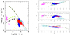 |
Fig. 4. Ie-Re plane and 3DKS of SSP galaxy models with with the MRR of Eq. (15), i.e., the Cosmic Galaxy Shepherd. The specific intensity Ie in use is for the B-passband. Left panel: the Ie-Re plane for the case with the constant ratio m = MDM/MS = 25, and the SFH described in the text. The black squares are the GLO-models while the dark olive green squares are the GAL-models. The small dots are the data of Burstein et al. (1997) and Illustris using the same color code of Fig. 1. In the same panel we also show GLO-models in which the ratio m = MDM/MS = 5. See the text for more details. Right panel: the corresponding 3DKS. Symbols and color codes are the same as in the left panel. The GLO-models for m = MDM/MS = 5 are not displayed because the difference with respect to those with m = MDM/Ms = 25 is very small. |
Basic quantities of the analytical model galaxies in the kappa space.
An inspection of Fig. 4 allows us to note several interesting points. First, in looking at the Ie-Re plane, the GLO-curve (if prolonged) seems to cross the GAL curve at log Ie ≃ 3 and log Re ≃ 3.8, that is, at GAL model with log Ms = 11.6 (i.e., log MDM = 13). In addition, the GLO line would provide an upper limit to all the observational data for galaxies and also the Illustris models, with the exclusion of globular clusters that are only marginally matched by this line. There are three possible causes of disagreement: the luminosity of the SSPs assigned to a globular cluster of a certain mass, the MRR in use, and, finally, the mass Ms assigned to an object of mass MDM (the ratio m = MDM/Ms). To assign the luminosity to a SSP representative of a real object we have used the magnitude vs. age relationship that has been derived from averaging the relationships for SSPs of different metal content (from Z = 0.0001 to Z = 0.07). By doing this for globular clusters, objects of low metallicity, we underestimated their integrated magnitudes, MB and MV, by about half a magnitude, corresponding to about a factor of about 1.6 in the luminosity (which is about a factor of 1.6 lower than the real value). A factor of 1.6 in luminosity, while keeping the radius fixed, would translate into an upward shift in the log(Ie) of about 0.2, which is too small to reconcile theory and data. The adopted MRR fits the bulk of globular clusters in the MR plane (see Fig. 2). Some adjustments are possible, but there is no room for big changes. Variations in the ratio m = MDM/Ms) are more promising. To this aim, recalling that globular clusters are commonly thought to be dark matter free or much less abundant than in other type of objects (Montes et al. 2020), we decreased m = MDM/Ms from 25 to 5 (third group of models in Table 4). They are displayed on the left panel of Fig. 4 by the green triangles. They have the same properties of the previous ones, namely: the mass, Ms, is larger, the radius Re derived from Eq. (15) remains unchanged, the surface brightness, Ie, is about a factor of ten higher, the globular clusters are matched, and the intersection with the GAL curve is expected now to occur at about 12.5 < log MDM < 13.5 M⊙, that is, 11 < log Ms < 12 M⊙. Based on this premise, it is worth noting that all data are bounded towards the highest surface brightness by the GLO curve up to the intersection with the GAL-curve and by this latter afterwards. No object is seen above this limit. Below this limit all other objects are found going from star clusters to dwarf galaxies, LTGs and ETGS and even galaxy clusters. The drop-like area crowded by intermediate mass galaxies (9.0 ≤ log Ms ≤ 10.5 M⊙, with a radius in the range of 3 ≤ log Re ≤ 4 pc in the Illustris sample) is partly due to mass resolution of these large-scale simulations (at the small radii side) and partly to the onset of the MRR for ETGs (on the large radii side). The combined line (GLO up to log Re ≃ 4 and GAL afterwards) in the Ie-Re plane is the analog of the MRR in the MR plane of Fig. 2. As anticipated, the MRR of the Cosmic Shepherd refers to objects in mechanical equilibrium and in passive evolutionary stage, in other words, to the line limiting the zone of avoidance in the MR- and Ie-Re planes.
Next, we turn to the projections of the 3DKS shown in the right panel of Fig. 4, where the same observational data and models of the left panel are plotted using the same symbols and color code. The right panel is in turn split in three sub-panels for the k3-k1 plane (top), k2-k1 plane (middle), and k3-k2 plane (bottom). We do not plot the GLO models with m = MDM/Ms = 5, because in the 3DKS, the difference with respect to those with m = MDM/Ms = 25 is negligible, namely, it is only a small horizontal shift in the middle panel. The panel that is of particular interest is at the top, displaying the classical fundamental plane. As expected, the GLO line and the GAL line only provide boundaries to the observational data plotted on the three planes: in the k3-k1 plane (top panel) the GLO line agrees with the upper values of data, while GAL line nicely reproduces the slope of the fundamental plane; in the k2-k1 plane (middle panel), the GLO line is the upper boundary to globular clusters, dwarf galaxies, and low-mass galaxies, while the GAL line is the upper boundary to high mass galaxies and galaxy clusters; in the k3-k2 plane (bottom panel), all the data collapse toward a thick strip whose mean slope coincides with that of the models. There is an offset that can be attributed to the crudeness of the models. In conclusion, there seems to be general agreement between data and theory.
Finally, based on the improved results obtained for the GLO-models using the ratio m = MDM/Ms = 5, instead of setting a fixed value for all models, we allowed the ratio to vary with the mass, MDM, as predicted by the NB-TSPH simulations. Therefore, we adopted the relation of Eq. (18), according to which m decreases from 23 for log MDM = 15 to about 6 for log MDM = 6. The results are shown in Fig. 5. Apart for a few minor details, they are nearly identical to those of Fig. 4. Based on these results, we learned that the parameter m (although it does play a key role) is not the main player in determining the shape and details of the Ie-Re plane and the 3DKS.
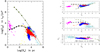 |
Fig. 5. Same as in Fig. 4. Left panel: Ie-Re plane. Right panel: 3DKS. The physical assumptions for the SSP-models and meaning of the symbols are the same as in Fig. 4. The only difference here is that we adopt ratio MDM/Ms given by Eq. (18) to calculate the SSP-models. |
We also repeated the above analysis using different MRRs, namely the empirical MRR derived from the sample of ETGs of Bernardi et al. (2010) and the semi-theoretical MRR of Fan et al. (2010). We found that the data-model agreement is not as good, compared to the MRR of the Cosmic Galaxy Shepherd (more detailed results are presented in Appendix A). Here, we prefer to focus on the MRR we have adopted. It is worth recalling that by construction this MRR refers to objects that are very close to mechanical equilibrium (virial condition) in which neither mergers nor galactic winds nor gas stripping or mass removal have occurred in the recent past. Since galactic wind are usually the result of intense star formation, our MRR is suited to describe situations in which star formation is either very low or has ceased in the past. As a consequence, the MRR in use is not suited to objects in which star formation is active, as in the case of DGs usually having star formation in repeated bursts of activity. In summary, our MRR cannot account for galaxies far from the above ideal limit. Simulations of these cases can be made using for low mass galaxies the MRR suggested by DGs which runs flatter than our MRR, that is, larger radii would correspond at a given Ms; in other words, an MRR similar to that of Fan et al. (2010) or that of Burstein et al. (1997) and Geha et al. (2006) for DGs and low mass ETGs (see details in Table 1) could be more suited to low-mass model galaxies. The issue is examined in the context of the infall models below.
6.1. More on the SFH
The above analysis also yielded an idea of the kind of SFH that occurred in the various groups of objects. Looking at our best case, that is, with the MRR of the Cosmic Galaxy Shepherd and m varying with MDM (according to Eq. (18)), the intersection between the GLO line and the GAL line occurs at about log MDM = 13.2 or, equivalently, log Ms ≃ 12. With this value for Ms, we can estimate the mean V and B magnitudes of the stellar content, MV ≃ 3.68 and MB = 4.36. Inserting these values into the magnitude vs. age relationships of Fig. 3, we estimated the age at which star formations ceased in the galaxy rest-frame. Both magnitudes yield a similar age interval 9.2 ≤ log Tstar ≤ 9.7. Using the age of the universe of 13.8 Gyr, this occurred in the age interval from about 12.4 to about 8.8 Gyr ago, corresponding to redshifts of roughly 4.5 to 1, respectively. Considering the crudeness of the current estimate, the result is consistent with the analysis of the cosmic star formation rate by Chiosi et al. (2017) in which the peak of activity is confined in the redshift range 2 to 1. The key assumption of our SFH is that both in GCs and ETGS, it mainly took place very early in the past. If in GCs that star formation ceased long ago is commonly accepted, this is not always true in ETGs. For the fact that the stellar content of ETGs indicates very old ages, this is somehow in contrast with the hierarchical building up of galaxies by repeated mergers most likely accompanied by star formation. Although ways out have been suggested (e.g., dry mergers), in our opinion, the controversy is more formal than real for the following reasons. Given that low-mass objects are far more numerous than the high-mass ones, the former are natural candidates for establishing the key building blocks at work. At beginning of the star forming process, mass accretion occurred among objects of comparable mass so each event implied a significant change of the chemo photometric properties of the mass growing objects (mass, radius, velocity dispersion, chemical composition, luminosities, colors, etc.). As time progressed and the mass of a galaxy increased, the impact of each accretion event became more and more irrelevant and, at the same time, mergers among objects of comparable mass became less and less probable, thus leaving the accreting object nearly unchanged. This may easily explain why ETGs look old even if they may have accreted some amount of mass in the recent past. The analysis of the color-magnitude diagram of ETGs (integral quantities) by Sciarratta et al. (2019) has amply confirmed this interpretation.
If the above picture of the present SFH is abandoned and other temporal prescriptions are adopted (e.g., Tsfr always increasing or decreasing, or constant) we cannot simultaneously fit both the Ie-Re plane and the 3DKS planes. This made evident when looking at the partial solutions shown by the GLO and GAL lines. Only the combination of the two types of SFH yields acceptable results. Other assumptions for Tsfr have been explored with negative results, but these are not shown here for the sake of brevity.
6.2. Dispersion of the MRR: Physical implications
In the above simulations, we adopted MRRs without considering whether they 1) have an intrinsic dispersion, 2) contain a parameter that is to be fixed by other constraints, or 3) represent ideal limits separating the permitted regions from forbidden ones. More precisely, the empirical MRRs of Bernardi et al. (2010) and Burstein et al. (1997) have an intrinsic dispersion of about 0.75 in log Re at given log Ms; the Fan et al. (2010) MRR contains the redshift of galaxy formation, zf, as a parameter and therefore galaxies born at different epochs should populate a strip with a certain width on the MR plane. Finally, the Cosmic Galaxy Shepherd is an ideal limit toward which all systems tend to crowd as they evolve toward the condition of mechanical equilibrium and inactive star formation. Also, in this case, a curved strip with a certain width is expected. In addition to it, the theoretical models of Illustris show a broad ranges of possible radii for a given mass. On the observational side, from globular clusters to galaxy clusters, real objects tend to occupy a broad slightly bending strip on the MR plane. To quantify the above statements, we estimated the thickness of the observed distribution on the MR plane along the radius axis per group of objects. The data are collected in Table 3, labeled as Δlog Re, max. Starting from this and keeping fixed the mass (both MDM and Ms), we varied the original radius Re, o of the adopted MRR by the quantity Δlog Re = ran * Δlog Re, max where ran is a random number from 0 to 1. The new radius is:
 (28)
(28)
It is worth emphasizing here that with this experiment we are not evaluating the uncertainty affecting the position of each object in the various diagnostic planes, caused by the observational uncertainty on Re, o, but to examine whether GLO-and GAL-models can account for the observational distribution in the various planes due to fact that galaxies of the same stellar could have different radii (this is particularly true for galaxies of low mass, from 108 to 1010 M⊙). So far, the GLO and GAL models have only given the edge of the distribution. In this context, the relation in Eq. (28) fits our purposes. The results for the Ie-Re plane and the 3DKS are shown in Fig. 6. Looking at the locus on the Ie-Re plane (left panel), given by the GLO line continued after the intersection by the GAL line the region underneath, is populated by the models (in agreement with observational data). The models are presented for discrete values of the mass, MDM, and, hence, Ms and radius, Re, o, but thanks to the artificial dispersion on Re, they scatter along the vertical axis, that is, the surface brightness, Ie. More realistic simulations are not needed because the effect of the scatter (for whatever reason) has already been captured. More realistic models would simply blur the distribution of model galaxies in the plane. The region between the GAL and the GLO lines at the left-hand side of the intersection is also populated by models. However they are not of interest here because they would correspond to objects of low mass and very long ever increasing duration of star formation, that do not find an observational counterpart (they could correspond to the past evolutionary stages of galaxies of the same mass that however for obvious reasons are not plotted in this plane). Indirectly, this lends much support to the kind of SFH we have adopted. Moving on to the right panel, we see the effect of the radius dispersion of the 3DKS. In the top panel showing the relation k3 vs. k1, there is no effect at all. This can be understood in the context of k1 ∝ Ms and k3 ∝ Ms/L. Another noteworthy is that the GAL line matches the inclination of the FP well. The middle panel shows the relation k2 vs. k1, where  . In this case, the scatter on Re is evident thanks to the dependence of k2. The data are compatible with the combination of GLO models up to the intersection of the GLO and GAL lines and the GAL models afterwards. The models in between the two lines at the left-hand side of the intersection (the black circles) are the same as the correspondent ones on the Ie-Re plane and do not find observational counterparts. They can be discarded. Finally, the bottom panel shows the k3 vs. k2. Galaxy clusters fall on the left side of the panel. Most of the black circles at the right hand side are the models falling in between the GLO and GAL lines and can be discarded for the same reasons as above. Also in this case there is a general agreement between data and models. The M/L ratio steadily decreases passing from galaxy clusters to ETGs. Among galaxies, the highest values are those obtained for globular clusters and the GLO models.
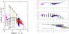 |
Fig. 6. Same as in Fig. 4. Left panel: Ie-Re plane. Right panel: 3DKS. The physical assumptions for the SSP-models (the blue squares and solid lines) and meanings of the symbols are the same as in the previous figures. The ratio MDM/Ms is given by Eq. (18) and therefore varies with mass, MDM, and the MRR is that of the Cosmic Galaxy Shepherd. The only important difference is that both in the GLO and GAL models the radius predicted by the Cosmic Galaxy Shepherd is increased by a random quantity within the range indicated in Table 3 and Ie is accordingly decreased. In the left panel the results are plotted as a function of the reference radius to highlight the fact that the radius is changed at constant mass. The experiment is meant to show that the areas delimited by the GLO and GAL models can be populated by objects with a radius larger than the MRR of the Cosmic Galaxy Shepherd. All the models in the area comprised between the GLO and the GAL lines have no physical counterparts and should be discarded. The same considerations apply to the 3DKS shown in the right panel. |
6.3. Considering the SFH or the radius as the star player
It is interesting to consider whether the curve in the Ie-Re plane and the behavior of models in the 3DKS are driven by the star formation history or the mass-radius relationship. To this aim, we supposed that the SFH is represented by the law, whereby the duration of the star formation activity ΔTsfr is ever-increasing with the galaxy mass. This case would nicely mimic the hierarchical scheme of galaxy formation. The results are shown in the left panel of Fig. 7 (solid black lines and black filled squares), where the physical assumptions for the SSP models and meaning of the symbols are the same as in Fig. 4. For sake of comparison, we also plotted the curve for an always decreasing ΔTsfr (green solid line and green filled squares). In the first case, while the upper border of the observational data on the Ie-Re plane is still reasonably matched (apart from for the most massive ETGs and galaxy clusters), serious difficulties arise with the 3DKS; in particular, with the k3 vs. k1 plane, where the distribution of ETGs and the FP are not fitted at all. What we would infer from this experiment is that the radius is the most important driver of the Ie-Re distribution. However, looking closely at the results, we note that the presence of an ever decreasing ΔTsfr term is unavoidable in order to properly explain the position of most massive ETGs and galaxy clusters. In the hierarchical scheme of galaxy and cluster formation, this would mean that activities such as the recent acquisition of new material (small objects on single galaxies or more galaxies on clusters of galaxies) and subsequent stellar activity are becoming less and less probable as time goes on.
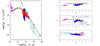 |
Fig. 7. Same as in Fig. 4. Left panel: Ie-Re plane. Right panel: 3DKS. The physical assumptions for the SSP-models and meaning of the symbols are the same as in Fig. 4. The only difference here is that the duration of the star formation activity ΔTsfr is supposed to always increase with the galaxy mass (solid black lines and black filled squares). This case strictly mimics the hierarchical scheme of galaxy formation. For sake of comparison, we also plot the curve for a constantly decreasing ΔTsfr (the green solid line and green filled squares). In the first case, while the upper border of the observational data on the Ie-Re plane is still reasonably matched (but for the most massive ETGs and galaxy clusters), serious difficulties occur with the 3DKS, in particular: with the k3 vs. k1 plane, where the distributions of ETGs and the FP are not fitted at all. |
6.4. Tightening up our constraints
The most important result of the previous analysis is that the distribution of stellar complexes going from globular clusters to galaxies (DGs, LTGs, ETGs) and even galaxies clusters, whose total stellar masses span eleven orders of magnitude, in the Ie-Re plane and 3DKS, they are delimited by a unique curve given by the combination of the GLO and GAL lines. As already stated above, the intersection occurs at about log MD ≃ 13 or Ms ≃ 12. In the left panel of Fig. 8, we show our best combination of the two lines. The resulting curve is compared with the data of Burstein et al. (1997); with the exception of globular clusters, all other objects are perfectly bounded by the curve. This line is the boundary splitting the Ie-Re plane in two regions: the permitted one under the curve and the forbidden one above it. The globular clusters seem to disobey the general rule; the cause may be either: 1) the ratio m ≃ 5, which should be lower; 2) the real luminosity, which could spread around the mean value we have assigned; or 3) some effects of dynamical nature on their radii that are not taken into account in this simple approach. We limited ourselves to the explanation of the curve falling somewhere in their region of existence. In the right panel, we show the 3DKS; in each panel the full black dots joined by a solid line show the curve. In the top panel the dashed line visualizes the FP of the models (k3 = 0.16k1 + 0.70) in the same region of the FP of ETGs of the Virgo and Coma clusters by Burstein et al. (1997), k3 = 0.15k1 + 0.36, the slope is the same, while the zero point is roughly a factor of 2 greater. This difference can be easily explained by considering that our border line is above the data for real ETGs (by construction because the models are based on the Galaxy Cosmic Shepherd for the MRR), while the observational FP is the best fit of the data for ETGs. We venture to state that the two relationships are in agreement. In the middle panel, the dashed line is the ZOE by Burstein et al. (1997), k2 + k1 = 8. Also, in this case, the boundaries are in solid agreement.
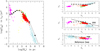 |
Fig. 8. Combined relationship for GLO and GAL models together. Left panel: Ie-Re plane in which the combined relation is shown against the observational data of Burstein et al. (1997). Right panel: corresponding 3DKS for the same models. In both panels, the meaning of the symbols is the same as in previous figures. No particular remarks are to be made here, aside from noting a general agreement between data and theory. The kind of SFH we have adopted seems to be compatible with the overall observational situation. |
7. Considering whether models of galaxies with infall perform better
An obvious criticism to the above analysis it that it stands on very crude approximation of a galaxy and its past history of star formation. Since NB-TSPH simulations of galaxy formation, both in monolithic and hierarchical scenarios, are beyond the aims of this study, we resort here to the so-called “infall” models that nicely mimic the collapse of a proto-galaxy and its gradual building up by mass accretion. Thanks to their simplicity, models of this type have been widely used in the literature to investigate a large number of different astrophysical problems. Originally developed by Chiosi (1980), they have been extended and improved by Tantalo et al. (1998), and recently used by Chiosi et al. (2017) to study the cosmic star formation rate and by Sciarratta et al. (2019) to investigate the galaxy color-magnitude diagram.
In brief, a galaxy of total mass MT is made of baryonic (BM) and dark matter (DM), with masses of MBM and MDM, respectively, and satisfying, at any time, the following equation:
 (29)
(29)
where baryonic and dark matter are present in proportions that are fixed by the adopted cosmological model of the Universe. The baryonic mass is supposed to be originally in form of gas, to flow in at a suitable rate and, when physical conditions allow it, to transform into stars. At the same rate, dark matter is also allowed to flow in together with the baryonic matter to build up the total gravitational potential. To this aim, a suitable prescription is adopted to describe the spatial distribution of baryonic and dark matter (we refer to Tantalo et al. 1998, or all details). Gas accretion by infall and gas consumption by star formation coupled together give rise to a time dependence of the star formation rate closely resembling the one resulting from the N-body simulations (e.g., Chiosi & Carraro 2002; Merlin & Chiosi 2006, 2007; Merlin et al. 2012). At any time, t, the baryonic mass, MBM, is given by the sum:
 (30)
(30)
where Mg(t) is the gaseous mass and Ms(t) the star mass. At the beginning, both the gas and the star mass in the proto-galaxy are zero, Mg(t = 0) = Ms(t = 0) = 0. The rate of baryonic mass (and gas in turn) accretion is driven by the accretion timescale, τ, according to:
 (31)
(31)
where τ is the accretion timescale and MBM, τ a constant with the dimensions of [mass/time] to be determined by imposing that at the galaxy age, TG, the total baryonic mass of the galaxy, MBM(TG), is reached:
![Mathematical equation: $$ \begin{aligned} {M}_{\mathrm{BM},\tau } = \frac{M_{\rm BM}(T_{\rm G})}{\tau [1 - \exp (- T_{\rm G}/\tau )]}. \end{aligned} $$](/articles/aa/full_html/2023/10/aa47000-23/aa47000-23-eq35.gif) (32)
(32)
Therefore, by integrating the accretion law, the time dependence of MBM(t) is:
![Mathematical equation: $$ \begin{aligned} { M_{\rm BM}(t) = { \frac{M_{\rm BM}(T_{\rm G})}{[1-\exp (-T_{\rm G}/\tau )] } } [1 - \exp (-t/\tau )] }. \end{aligned} $$](/articles/aa/full_html/2023/10/aa47000-23/aa47000-23-eq36.gif) (33)
(33)
The timescale, τ, is related to the collapse time and the average rate of gas cooling. Therefore, it is expected to depend on the mass of the system. Finally, dark matter flows in at the same rate as the baryonic matter, but it does not affect the evolution of the galaxy – apart from its effect on the gravitational potential energy.
The gas mass not only increases by infall but also decreases by star formation. To keep the model as simple as possible, we assumed that the rate of star formation is proportional to the available gas mass according to:
 (34)
(34)
where k = 1 and ν is the efficiency parameter of the star formation process. Based on the results obtained with the infall galaxy models, the relation in Eq. (34) turns out to be adequate to our proposes. In the infall model, because of interplay between gas accretion and consumption, the rate of star formation starts low, reaches a peak after a time approximately equal to τ, and then declines. The functional form that could mimic this behavior is the time delayed exponentially declining law:
 (35)
(35)
The Schmidt law in Eq. (34) therefore represents the link between gas accretion by infall and gas consumption by star formation.
As a whole, this kind of approach stands on a number of observational and theoretical arguments among which we recall: (i) the parameters ν and τ can be related to morphology (Buzzoni 2002) and to the presence of ongoing star formation activity inside observed galaxies (Cassarà et al. 2016; ii) the aforementioned quantities can be easily tuned in order to fit observational data, and also complex phenomena that would affect the rate of gas cooling, such as active galactic nuclei (AGN), can be empirically taken into account (see e.g., Chiosi et al. 2017). These galaxy models include many important physical phenomena, such as gas heating by supernova explosions (both type Ia and type II), stellar winds, gas cooling by radiative emission, galactic winds, and the presence of DM in shaping the gravitational potential (required in the presence of galactic winds). We refer to the study by Tantalo et al. (1998) for all details on these topics. The list of the key model parameters used in this study is given in Table 5. The models are labelled by their baryonic mass, MBM, which is, in turn, produced by the stellar mass, Ms, and the gas mass, Mg (at the beginning only gas, at present mostly stars and little gas left over). The input parameter of the models required to specify the accretion rate (the timescale, τ) and the SFR (with the exponent, κ, and specific efficiency, ν) are listed in Table 5.
Key parameters of model galaxies: MBM(TG), ν, and τ.
At each time, t, we evaluated the radius Re of the stellar component Ms by means of the MRR of Fan et al. (2010), as per their Eq. (15). To determine the radius, we need to know the amount of dark matter present in the galaxy at the time, t. Since MDM is supposed to fall at the same rate as MBM, it ought to obey a relation similar to that of Eq. (33), where MBM(TG) is replaced by MDM(TG). However, a simple estimate of MDM(t) can be derived from Ms(t). At the beginning (t = 0), the ratio MDM/MBM is in cosmological proportion, and with the adopted cosmological model of the Universe, MDM/MBM ≃ 6. As the evolution of the proto-galaxy proceeds, both Ms grows from zero to a significant fraction of MBM. Current NB-TSPH models (Chiosi & Carraro 2002; Merlin et al. 2012) suggest that Ms ≃ 0.3MBM (the rest of the gas is likely dispersed by galactic winds), which yields the mean value MDM/Ms ≃ 20. Knowing Ms, then MDM follows and, thus, Re can be calculated. Finally, the luminosity of the galaxy as a function of time can be calculated with the population synthesis technique described in Bressan et al. (1994), so that the detailed star formation history is taken into account.
Three series of models were considered: (i) in the first group, there was no constraint on star formation activity, which never stopped over the course of evolution. Although it was reduced to minimal levels of activity, star formation is also active at the present age; (ii) in the second group soon after the activity peak (approximately soon after the age t ≃ τ, when the bulk of stars is already in place) star formation was stopped. Consequently, at the present age, the light emitted by the galaxies is free from contamination from newly formed stars. This allows us to evaluate the effect on the luminosity (and Ie in turn) based on ongoing star-forming events. We evaluated the decrease in luminosity Δlog(L/L⊙) in the range between 1 and 2 and we took the lowest value as a minimum estimate; (iii) in the third group, we examined the effect of the MRR. While massive galaxies (masses greater than about 1010 M⊙) at the present time obey a sharp MRR, this is not the case with respect to less massive galaxies, whose Ms and Re are apparently weakly correlated. They do indeed crowd in a cloud on the MR plane, although a weak correlation can be derived (see Chiosi et al. 2020, for a thorough discussion of this problem). To this aim, we calculated a third group of models in which the MRR for less massive galaxies is taken from Woo et al. (2008), which is much flatter (about a factor of two) than the one adopted for the more massive galaxies3.
The results are shown in Fig. 9, where the right panel is the Ie-Re plane, while the right one the 3DKS. Looking at the left panel, the blue lines are for the models with the standard MRR and no constraint on the SFR, while the red lines are for those with an interrupted SFR. In the same figure, the green and magenta models are the same (green for active star formation and magenta for extinguished star formation) for low-mass objects with a flatter MRR.
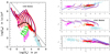 |
Fig. 9. Same as in Fig. 4. Left panel: Ie-Re plane of the model galaxies with infall. The mass MBM(TG) grows from left to right in steps of a factor of 10 from 106 to 1013 M⊙. The infall timescale, τ, and specific efficiency, ν, of star formation are listed in Table 5. The MRR relation is from Chiosi et al. (2020), the Cosmic Galaxy Shepherd. The blue lines are models with active star formation all over the evolutionary history. The red lines are models in which star formation is quenched off past the age t ≃ τ. The green and magenta lines indicate model with active (green) and quenched off (magenta) star formation, but in which the MRR relation for galaxies with stellar mass in the interval 106–109 M⊙ is that of the dwarf galaxies of Woo et al. (2008). See the text for more details. Right panel: Projections of the 3DKS. In each sub-panel, all the symbols have the same meaning as in the left panel. In each line the final stage (present age) is close to the observational data. It is worth noting that in the k3 vs. k1 plane the relation passing through all the final stages of the models with quenched star formation at the present age perfectly coincides with the FP plane of ETGs in the Virgo and Coma clusters. |
Looking at the first and second group (i.e., models with standard MRR and different star formation rates) it is worth recalling that a galaxy move along this line from the top to the bottom at decreasing speed because the variation in luminosity slows down as the evolution proceeds. The present age is the last point of each line. The distribution of the final stages mimics the upper boundary of the distribution of observational data in the Ie-Re plane. To this aim, we also plot the composite GLO plus GAL line (the black full squares joined by a solid line). The two boundaries coincide. Remarkably, all the final points of the blue lines fall either along or below the ZOE border, those of the red lines are well below this. The obvious implication is that the effect of star formation cannot be ignored when examining the properties of the Ie-Re plane.
Moving on to the third and forth groups (models with shallower MRR for less massive galaxies, but different histories of star formation; i.e., green ones with active star formation up to the present time and magenta ones with quenched stellar activity), we find that thanks to their larger radii at a given Ms, they greatly shift toward lower Ie and higher Re values. Since, from the observational point of view, galaxies in this mass range show radii, Re, in the range predicted by Chiosi et al. (2020) and Woo et al. (2008), the terminal stages of all models presented in Fig. 9 encompass all reasonable situations that can be seen at the present time in this diagnostic plane.
Finally, these models provide an idea of the spread to be expected because of a spread in the epoch of galaxy formation (nowadays, galaxies would be detected in different evolutionary stages), different star formation histories, and different histories of their dimensions caused by internal (galactic winds) and external (merger) events. They also strongly confirm the idea that the most massive galaxies ceased their star formation histories long ago. Moreover, these results are in perfect agreement with the observational data presented of Fig. 1.
To conclude, all these results lend strong support to the notion that the ZOE is traced by galaxies in virial equilibrium and passive internal evolution. They also suggest that ZOE is not the same at all times but the boundary may change as time goes on. Part of the evolutionary history of massive galaxies (when their mass is built up via the acquisition of surrounding material) could indeed be spent beyond the border of the present day ZOE. This point will also be confirmed by analyzing the Ie-Re plane at different redshifts. Moving on to consider the 3DKS in the right panel of Fig. 9, we find the infall models confirm the results obtained with the SSP-models.
8. Ie-Re plane and 3DKS back in time: Role of redshift and mergers
To cast light on the properties of the Ie-Re plane and 3DKS (and its projections) in the past and how they evolved to the present morphology, we used the Illustris data. In the left panel of Fig. 10, we display the Ie-Re plane for four selected values of the redshift, namely, z = 4, z = 2, z = 1, and z = 0. In this diagram, we also show the GLO and GAL lines of the reference case at the present time. Along each line, the squares visualize the position of the GLO- and GAL-models listed in Table 4. The distribution of the Illustris galaxies is clumpy and irregular at high redshifts independently of the galaxy mass. Starting from z = 1 and more evident at z = 0, a tail-like feature develops at the side of large masses, at around ≳1 − 2 × 10¹¹ M⊙. The tail-like structure develops for the first time starting from z ≃ 1.2 or so when also the MRR for ETGs sets in, see Chiosi et al. (2020) for an extensive analysis of the MRR of these galaxies.
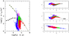 |
Fig. 10. Evolution of the Illustris galaxies on the Ie-Re plane (left panel) and the 3DKS (right panel) from z = 4 to z = 0. There are four values of the redshift with the following color code: blue (z = 4.0), magenta (z = 2), green (z = 1), and red (z = 0). In the left panel, we also display the GLO and GAL lines of the reference case. The right panel is split in three parts showing the correlations k3 vs. k1 (top), k2 vs. k1 (middle), and k3 vs. k2 (bottom). In the k3 vs. k1 plane, which shows the fundamental plane, we also plot the relation derived by Burstein et al. (1997) for ETGs in the Virgo and Coma clusters (k3 = 0.15k1 + 0.36, dashed line) and the same for the Illustris objects falling in the region of ETGs of the MR plane (k3 = 0.20k1 − 0.075, solid line). The agreement is fairly good. In the middle diagram we also plot the ZOE line given by Burstein et al. (1997) with the equation: k2 + k1 = 8. |
Key questions in this regard include: 1) the reason behind the cloud-like and tail-like distributions; 2) why the cloud-like one dominates in the low mass range and at high redshifts, when the opposite seems to happen for the tail-like one, which shows up in the high mass range and at low redshifts; 3) what the physical meaning is behind these two distributions. Some of these issues have addressed by Chiosi et al. (2020) in a discussion of the nature and physical origin of the MRR. In the following, we go over these questions once more, framing them in the wider context of galaxy evolution with redshift.
The Illustris simulations are based on the hierarchical scheme, therefore, each galaxy is the result of a number of processes involving mass acquisition and/or removal, which affect the masses, radii, velocity dispersion, and luminosities of a galaxy. For each galaxy in the sample at z = 0, the Illustris database provides the past history, namely, the masses and radii of the components sub-units during the Hubble time. This means that we can reconstruct the past history in the Re vs. Ms plane of each galaxy from z = 4 to z = 0. Chiosi et al. (2020) inspected a number of cases chosen from the whole sample and reconstructed the path on the MR plane throughout their evolutionary history. The results can be summarized as follows: (i) the path of each galaxy is quite tortuous: in general, both mass and radius increase, but often either the mass or the radius or both decrease; (ii) mergers among objects of low and comparable mass yield objects that remain inside the cloud, while mergers among objects with relatively high mass tend to generate objects that leave the cloud and fall along a well behaved MRR identical to that of today ETGs; (iii) the cloud-like region roughly coincides with the region crowded by DGs of different type. However, a careful inspection of the Illustris models reveals that also among DGs, a number of them in the z = 0 group fall along the MRR of ETGs, for instance, near the position of galaxies such as ωCen and M32. Star formation in these DGs is either not quenched at all or only at minimal levels, as in ETGs. Thus, it seems that low mass galaxies can exist while sharing the same equilibrium conditions of the massive ones; (iv) a hint arises to suggest systems that are in mechanical equilibrium and passive evolutionary state belong to (actually give rise to) the MRR; (v) given the mass of a galaxy (either acquired by mergers or already in place ”ab initio“), the radius mirrors the condition of mechanical and thermal equilibrium of the system. In other words, the radius is determined by the energy balance between the dynamical collapse and feed-back by star formation. A key aspect in this context is the role of galactic winds, which are found to be stronger when star formation is stronger. Chiosi et al. (2020) attributed to intense star formation and presence of strong galactic winds the large departure of DGs from the ideal MRR, thus accounting for their cloudy distribution on the MR plane.
Similar results have also been suggested by the evolution of the tail-like structure on the Ie-Re plane with cosmic time (see the left panel of Fig. 10). This characteristic feature appears only at redshifts lower than about 1.2.
In the right panel of Fig. 10, we show the correlations k3 vs. k1 (top), k2 vs. k1 (middle), and k3 vs. k2 (bottom). In the top panel, we see how the fundamental plane of ETGs (the tail of green and red points) develops at decreasing redshift (for redshifts smaller that about z = 1.2. For the sake of comparison we also show the fundamental plane of ETGs derived by Burstein et al. (1997) for ETGs in the Virgo and Coma clusters (k3 = 0.15k1 + 0.36, dashed line), together with its analog for the Illustris objects falling in the region of ETGs of the MR plane (k3 = 0.20k1 − 0.075, solid line). The agreement is fairly good. In the middle diagram we also plot the ZOE line given by Burstein et al. (1997), with the following equation: k2 + k1 = 8. In this case, the agreement is also good.
The inspection of the three sub panels at the right hand side of Fig. 10 immediately reveals that the FP in the 3DKS sets in at the same time (redshift) of the tail in the Ie-Re plane and the MR-relation of ETGs in the MR plane. All of this strongly suggests a tight connection between the MRR, the Ie-Re tail, and the FP.
To strengthen the above conclusions, in Fig. 11 we compare the observational data of Burstein et al. (1997) at z = 0 for ETGs (small red squares) and DGs (small green squares) with the theoretical models of Chiosi & Carraro (2002) calculated in the monolithic scheme for two different values of the initial density (redshift). The high initial density models (z ≃ 5) are indicated by the red triangles and the red dashed line, while the low density ones (z ≃ 1) by the blue squares and the blue dashed line. In all panels the empty circles show the position of M32 (NGC221). The solid black line in the k1 vs. k3 plane is the best fit of the models for ETGs, therefore showing the slope of the FP to be compared with that for ETGs in Virgo and Coma clusters. The equations for the FP are k3 = 0.14k1 + 0.41 for the models and k3 = 0.15k1 + 0.36 for the real galaxies. The agreement if fairly good. The position of M32 is always close to the models formed at high redshift, namely, in an environment of high initial density. Finally, in the background we also show the Illustris models at z = 4 (light-green dots). We note the striking difference of the galaxy distribution in the three planes at varying redshift. At high redshift, there is no trace of the classical FP derived from normal ETGs; massive ETGs in the Illustris sample are still missing. These galaxies begin to appear at redshift z ≃ 1.5 and their FP is nearly identical to that of the objects in Virgo and Coma clusters.
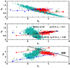 |
Fig. 11. 3DKS of ETGs (small red squares) and DGs (small green squares) of the Local Universe (hence, at the present age, z = 0) by Burstein et al. (1997). The data are compared with the monolithic models by Chiosi & Carraro (2002) for two formation redshifts and hence initial densities. The high initial density models (z ≃ 5) are indicated by the red triangles and the red dashed line, while the low density ones (z ≃ 1) by the blue squares and the blue dashed line. In all panels, the empty circle shows the position of M32 (NGC221). The solid black line in the k1 vs. k3 plane is the best fit of the models for ETGs, the slope of which nicely coincides with the slope of the FP for ETGs in Virgo and Coma clusters. The equations for the FP are k3 = 0.14k1 + 0.41 for the models and k3 = 0.15k1 + 0.36 for the real galaxies. The agreement if fairly good. In the background, we also show the Illustris models at z = 4 (light green dots). We note the striking difference of the galaxy distribution in the three planes at varying redshift. |
As already stated, the paradigmatic view of galaxy formation and evolution is through successive mergers of sub-units of different mass and luminosity. In this context, it is worth investigating how much the luminosity of individual objects is affected by repeated mergers and companion star formation activity, and, consequently, how much the luminosity variations affect the various diagnostic planes under investigation. To highlight the effect of mergers on the photometric properties of galaxies, D’Onofrio & Chiosi (2023b) proposed a toy model of merger in which starting from the mass and luminosity of the merging galaxies quick predictions for the luminosity of the resulting object are possible. We thus consider two galaxies with total stellar mass, M1 and M2, and total luminosity, L1, and L2, (either bolometric or in some band). The luminosity is generated by the stars already existing in each galaxy. The two galaxies are supposed to merge. The merger event may or may be not accompanied by star formation induced by the merger itself. We let Ms be the mass of gas (belonging to one of the galaxies or both) that is eventually turned in newly born stars. For simplicity, we consider this event as a unique single stellar population, SSP, of total mass, Ms, generating a total luminosity, Ls. If no star formation occurs at the merger, then Ms = 0 and Ls = 0.
The total mass of the system is M = M1 + M2 + Ms and the ratios between the mass of each component and the total mass are α1 = M1/M, α2 = M2/M, and αs = Ms/M. The total luminosity is L = L1 + L2 + Ls and the corresponding ratios between the luminosity of each component and the total one are h1 = L1/L, h2 = L2/L, and hs = Ls/L. We may order the galaxy masses as functions of their value, so that α1 > α2 > αs. As the luminosity of a galaxy depends not only on the mass but also on the age (the luminosity gets fainter as the age increases) and it may undergo large and fast variations in presence of star formation, thus, the sequence h1 > h2 > hs can be easily violated. It may happens that h2 > h1 and hs > h1 and/or hs > h2.
The initial luminosity of each component is generated by its stars. In other words, it is the result of the time integration of the star formation history of the galaxy. In a galaxy, supposing that each star formation event in the time interval, dt, can be represented by a SSP of suitable chemical composition emitting the total luminosity lssp(t), the total light, L, is given by  , where Ψ(t) is the current rate of star formation in suitable units, t, is the current age of the galaxy (at z = 0 t = TG), and lssp is the luminosity of the generic SSP (integrated over the mass interval spanned by living stars at a time, t.
Under typical assumptions for Ψ(t) in our galaxy models, the luminosity starts low, grows to a maximum and then declines. The peak occurs at the age approximately equal to the infall time scale τ. The interval spanned by L(t) is about a factor of 10 because of the double integration (over the mass for lssp and time for L(t), while that of SSP with the Salpeter IMF is more than a factor of 200. For more details, we refer to D’Onofrio & Chiosi (2023b).
In absence of star formation (Ms = Ls = 0), the merger is said to be “dry”, whereas in the presence of star formation (Ms ≠ 0, Ls ≠ 0), the merger is said to be “wet”. We let Ms be the mass of gas (belonging to one of the galaxies or both) that is eventually turned into newly born stars. For simplicity, we consider this event as a unique single stellar population, SSP, of total mass, Ms, generating a total luminosity, Ls. If no star formation occurs at the merger Ms = 0 and Ls = 0 and the merger is said to be “dry”. This is an important detail because the luminosity range and fading rate of a SSP are different from the same quantities when they are referring to the whole galaxy.
Stellar models and SSPs are taken from the Padua library of stellar models, isochrones, and SSPs (see Bertelli et al. 1994, 2008; Girardi et al. 1996; Nasi et al. 2008, for all details and ample referencing). The model galaxies are those already described in this paper and in D’Onofrio & Chiosi (2023b). The SSPs in use are for the Salpeter initial mass function with slope x = 2.35 (in number of stars per mass interval), the SSP mass is MSSP = 5.826 M⊙. In the following, we consider a few typical mergers. Masses and luminosities are in solar units and the effects due to differences in the mean chemical composition of the stellar contents can be ignored at a first order approximation.
Dry mergers (no additional star formation). With this assumption, we always have Ms = 0 and Ls = 0. Furthermore, we also have (a) the case of two identical objects (same mass, same stellar content, and same age) with, for instance, M1 = M2 = 1012 M⊙ and luminosity L1 = L2 = 1011 L⊙. The luminosities have been derived from the galaxy models at the present age. In this case, the mass and luminosity of the resulting object are two times the starting value (α1 = α2 = 0.5 and h1 = h2 = 0.5); (b) The case of two objects with different mass but same age (old). Supposing M1 = 1012, L1 = 1011, and M2 = 1011, L2 = 1010. The total mass is M = 1.1 × 10¹² and the total luminosity is L = 1.1 × 10¹¹. Therefore, α1 = 0.909, h1 = 0.909 and α2 = 0.091, h2 = 0.0.091. The light of the resulting object is dominated by the more massive galaxy. The merger has increased the total luminosity by about 10%. This can be considered a sort of upper limit because a dry merger between two galaxies of the same age that differ in mass by more that a factor of 10 would (in practice) be undetectable; (c) in the case of two galaxies with different mass and different ages, and thereby different luminosities, the total luminosity may show the effect of the younger object. Considering the following galaxies, M1 = 1012, L1 = 1011 (the old object) and M2 = 1011, L2 = 5 × 10¹⁰ (the young object, taken near the peak value). After merging, the total mass is M = 1.1 × 10¹², while the total luminosity is L ≃ 1.5 × 10¹¹. Therefore, α1 = 0.909, h1 = 0.667 and α2 = 0.091, h2 = 0.333. The contribution to the total mass by the younger less massive object is about 10%, while its contribution to the total light is about half that produced by the more massive but older object. Other combinations of masses and luminosities can soon calculated with similar results.
Wet mergers (additional star formation). In this case Ms ≠ 0 and Ls ≠ 0. The major difference with respect to previous cases is that the stellar activity induced by the merger can be approximated by a single giant SSP with its own mass and luminosity. The total light emitted by Ms is Ls = (LSSP/MSSP)×Ms. Now the interval spanned by the luminosity at aging SSP is much wider than before and so, depending on the age, the effects can be large. To illustrate the point for the merging galaxies we assume M1 = 1012, L1 = 1011, M2 = 1011, L2 = 1010, and finally for the mass of the giant SSP simulating the induced star formation event, we adopted Ms = 1010. The total mass is M = 1.11 × 10¹². For the associated luminosity, we adopted three values corresponding to a very young-age, high-luminosity SSP with Ls = 1 × 10¹¹; an intermediate-age, lower luminosity SSP with Ls = 1 × 10¹⁰; and an old-age, low-luminosity SSP with Ls = 1 × 10⁹. In the first case the total luminosity is L = 2.1 × 10¹¹, whose relative components are h1 = 0.476, h2 = 0.048, and hs = 0.476. The burst of star formation contributes to half of the total light and 1% of the total mass. This is a rapidly transient situation that ends up fading on a short timescale. In the second case, the total light is L = 1.2 × 10¹⁰, and the relative contributions to the luminosity are h1 = 0.834, h2 = 0.083, hs = 0.083; the burst of star formation contributes to about 10% of the light equal to the contribution of the less massive, old galaxy. In the last case, the SSP is very old, the three relative contributions are h1 = 0.908, h2 = 0.091, and hs = 0.009. The occurrence of the burst is nearly undetectable. Other combinations of the parameters can be tested with similar results.
What we have learned from these simple tests is that in the case of dry mergers, with the exclusion of a merger between objects of similar mass in which the mass and light are increased by a factor of two, the effect of mergers among objects with different masses and ages scarcely affect the light of the originally dominant object. Wet mergers with induced star formation more efficiently leave their fingerprints on the post-merger light of a galaxy. Unfortunately, the bright phase is of short duration, the timescale required for an SSP to evolve from a turnoff in the range of bright massive stars (say 20 M⊙ with a lifetime of a few Myr) down to a turnoff in the range of low mass stars (say below 2 M⊙ with a lifetime of about 1 Gyr) is rather short compared to the total lifetime of a galaxy. Therefore, it is more probable to catch a galaxy that has undergone a wet merge when the burst of star formation has already faded down to low luminosities.
These are interesting results that could explain: (i) The cloudy distribution of low mass galaxies in the Ie-Re plane and the three projection planes of the 3DKs; this is the result of the intense stellar activity combined with mergers among objects of comparable mass; (ii) the narrowness of the tail of massive ETGs in the Ie-Re plane, and the narrowness of the MRR and FP at the same time. In such a case stellar activity is often over or at minimal level, most of mergers occur among objects of much different mass, mergers among large mass objects are highly improbable. Finally if a merger occurs along with a revival of star formation and consequent burst of luminosity, this is an event of very short duration and little impact on the most massive object.
9. The fundamental plane in star-by-star photometry
In this section, we focus on the fundamental plane (FP) relation, as it provides the tightest constraint to the underlying formation mechanism of ETGs (Dressler et al. 1987; Djorgovski & Davis 1987; D’Onofrio et al. 2017). To this aim we make use of the NB-TSPH galaxy models of Merlin & Chiosi (2006, 2007), Merlin et al. (2010, 2012) and also Chiosi & Carraro (2002). For all details on these models the reader is kindly invited to refer to the original papers.
It is worth recalling that since some models have been calculated up to some final redshift z > 0, the time, Tlast, does not correspond to the present age of the Universe, tU, nor the real age of the galaxy, TG = tU − Tz, ini. Therefore, Tlast < TG. However, since all models assemble 99% of their stellar mass before z = 1, this is less of a problem because there is (in practice) no star formation from z = 1 to z = 0. The stars already in place get older and their luminosity fades down. These effects can easily be taken into account. Furthermore, the stellar particle of the NB-TSPH models is indeed a massive SSP with known mass, chemical composition and age, so that extrapolations of the luminosities and colors to the present day values can easily be evaluated.
The luminosity, LΔλ, in a certain band Δλ within Re is calculated as follows. In each model of our set, the star particles are centered on the barycenter and projected on the XY-plane, XZ-plane, and YZ-plane. In this way, we can take into account the deviation of the object from the spherical symmetry by means of the three different projections corresponding to three different positions of an external observer. Each star particle represents a SSP of metallicity, Z, born at the time, T, and with an age of τ = Tlast − T. The total luminosity in the B-band and the half-light radius Re in kpc are then obtained by subdividing the 2D projections in a fine grid of circular rings and adapting the population synthesis technique for N-body simulations presented in Tantalo et al. (2010). Since we tried to be as consistent as possible with the Burstein et al. (1997) estimates of masses and luminosities, the masses, Ms, inside the effective radius, Re, are derived from:
 (36)
(36)
where σc is the velocity dispersion in km s−1 the stellar mass in M⊙, and Re in kpc. This result was obtained by averaging over the particles within the central region inside Re/8. As a consequence of the gravitational softening, the estimates of the velocity dispersion in the innermost region of the models can be affected by a significant degree of uncertainty. This is because the velocities of the particles are not fully consistent with the real Newtonian accelerations.
A preliminary comparison was made with Burstein et al. (1997) data, whreby we limited ourselves to a summary of the main results without going into a detailed description. In the plane log(Ms/Ls)⊙ vs. log(Ms), the slope of the linear fit of the Burstein et al. (1997) data in the B-band is:
 (37)
(37)
and that of our models is:
 (38)
(38)
thus, they are nearly parallel, except for a slight offset along the Y-axis. In attempting to mimic the observational data, we introduced a 20% uncertainty on the theoretical estimate of the velocity dispersion σc: this is enough to make the fits almost coincident. Both fits have been obtained for the models with masses Ms > 1010 M⊙ therefore excluding the lowest mass models of our list because they still form stars at a significant rate. Indeed, its B-band mass-to-light ratio is much lower than for all other models. In any case, the observed and simulated mass-to-light ratios in the B band, M/LB, show a consistent behavior, increasing with galaxy mass, that might actually account for a large part of the tilt of the FP (e.g., Bolton et al. 2008).
Furthermore, the observed and simulated mass-to-light ratios in the B band M/LB agree and increase with the galaxy mass (the “tilt” of the FP; see e.g., Ciotti et al. 1996). This can be explained by considering the mean age of the dominant stellar population and implying that a decrease in the stellar masses would require significant populations of young stars. Our models do account for such a requirement and at the final simulated redshift, they lie in the region of the diagram populated by early-type galaxies.
The low mass models invert the trend and have high values of the M/L ratios at tlast compared with the intermediate mass models. Considering that in this mass range, the scatter in the observational data is very large, the location of the models on this diagnostic plane may be taken as reasonable. Dwarf galaxies are known to have large mass-to-light ratios (Mateo 1998), so these results are consistent with the observations.
Moving to the 3DKS of the Burstein et al. (1997) data and our models, the situation proceeds as follows. The k1 vs. k3 plane shows the FP seen edge on. The data were grouped according to the mass, that is, M ≥ 1010 M⊙ and M < 1010 M⊙. The linear best fit of our models limited to masses greater than 1010 M⊙ yields k3 = 0.1777k1 + 0.1604, which then need to be compared with the fit of the Burstein et al. (1997) data, k3 = 0.1567k1 + 0.3044. The slopes are nearly identical while there is an offset of a factor of two in the zero point. If we include a 20% uncertainty in the dispersion velocity, the vertical offset is ruled out. Possible explanation is that the softening of the gravitational force in the models leads to underestimate the velocity dispersion. Finally, we looked at the correlation between k2 and k1. As already noted by Chiosi & Carraro (2002), most of the galaxies follow the slope of (and remain below) the line k1 + k2 ≤ 8, while the sample of dwarf galaxies are distributed in a long tail with a slope similar to that of the theoretical models. In particular, the boundary line k1 + k2 ≤ 8 simply reflects that in the course of the Universe evolution the mean initial density and upper mass limit of proto-galaxies get lower and higher, respectively.
The same analysis was carried out using the SDSS observations of ETGs of Bernardi et al. (2010). In Fig. 12, we compare our models to the mass-to-light ratios obtained with SDSS observations. In particular, we focused on the r′ band, for which we adopted the magnitudes and effective radii derived from a combination of De Vaucouleurs and exponential profiles. In order to estimate the mass-to-light ratio, two choices were available for the mass: (1) the estimate of Bell et al. (2003); (2) the estimate of Gallazzi et al. (2005) using a combination of medium-high resolution spectra and different SFH. For all the details, we refer to Bernardi et al. (2010), in particular Appendix A and Sect. 2. We find a reasonable agreement with the Bell et al. (2003) mass determinations: the theoretical models yield log(M/L) = 0.1632 log(M)−1.367, whereas the data yield log(M/L) = 0.1143 log(M)−0.7828. A better agreement is achieved using the Gallazzi et al. (2005) masses, in the case the fit of the observational data yields log(M/L) = 0.1859 log(M)−1.629.
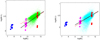 |
Fig. 12. M/L vs. M projection of the FP in the SDSS r′-band, i.e. the relation log(Ms/Ls)⊙ = log(M/Lr′)⊙ vs. log Ms, where log Ms is the stellar mass enclosed within the half-light radius, in units of 1012 M⊙ and calculated according to Bell et al. (2003; left) and Gallazzi et al. (2005; right). Lr′ is the r′ luminosity enclosed within the half light radius. The small dots in both panels are the data from the catalog by Bernardi et al. (2010; priv. comm.), whose linear fit is shown as a continuous line. The big filled circles refer to our sets of models (12 models × 3 projection planes = 36 models) and the best fit of the intermediate and high mass models is shown as a dashed line. The dispersion of the models along the vertical axis, in particular for the high mass ones, is mainly due to their different initial conditions. |
Finally, in Fig. 13, we show the FP for ETGs in the g′ and r′-bands for the data of ETGs (Bernardi et al. 2010). The agreement with the observations is good, once again when a ±20% correction in the dispersion velocity is applied. We note here a small difference in the slope between the fits to our models and observations in the k1 vs. k3 plane. In the k2 vs. k3 plane, the agreement is now better than for the B band, in particular, for the r′-band. The sample of Bernardi et al. (2010) contains almost sixty thousands galaxies with variable redshift, going from z = 0 to about z = 0.27, while our models have a final redshift going from z = 0 to z = 1. A more detailed analysis would require more simulations, particularly around log(Ms) ∼ 11, and to carry all the simulations up to z = 0.
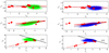 |
Fig. 13. Fundamental plane in the 3DKS for the SDSS g′ (left) and r′ (right) bands. In all the panels, the small dots are the elliptical galaxies of Bernardi et al. (2010). The meaning of the symbols is the same as in Fig. 12. |
10. Final remarks and conclusions
The main results of this study are as follows.
1. The simultaneous analysis of the Ie-Re plane and the 3DKS has proven to be an effective tool for reconstructing the history of star formation for a wide range of astrophysical objects, from globular clusters to galaxies. If we parameterize the SFH by the timescale of its duration, we find that the distribution of objects from GCs to ETGs (and also GCGs) can be explained by a SFH that was short in GCs, long in objects of intermediate mass from a few 106 M⊙ to a few 1011 M⊙, and short again above this mass range. A constant decrease or increase in SFH duration, independently of the galaxy mass, would lead to results that stand in contradiction to the observational data.
2. Only a certain type of relation between the stellar mass, Ms, and the half-light radius, Re, such as the Galaxy Cosmic Shepherd can explain the distribution of objects in the Ie-Re and 3DKS projection planes at the same time. Other MRRs would fail to do so, in the Ie-Re, in particular.
3. The question may arise with respect to whether it is the radius or the SFH that acts as the dominant parameter. The numerical experiments clarify that the radius serves the key parameter in the Ie-Re plane in particular, while the SFH strongly affects the behavior of the 3DKS projections.
4. The adopted prescription for the SFH duration determines a threshold line in the Ie-Re plane above which no object in virial equilibrium that is either extinguished or displaying very low star formation activity can exist at the present time (z = 0). On the side of such high-mass objects as massive ETGs and GCGs, this line coincides with ZOE, which has been introduced by Bender et al. (1992). We suggest extending the concept of ZOE limit to the new line. All observed objects are below this line in the Ie-Re plane and in the 3DKS projection planes.
5. Models with infall that somehow mimic the mass assembly and evolution of the hierarchical scheme do not affect the above conclusions. However, they clearly show that they can easily populate the regions below the threshold line (generalized ZOE line) but also (and even more relevant here) that in the past, they could have traveled in the forbidden area. This result has been confirmed by the Illustris models at higher redshifts.
6. Overall, the ZOE line can change over time and, hence, across redshift. Thus, the present-day forbidden area could be populated by galaxies in early epochs of active star formation, as suggested by the infall models and the Illustris simulations. This is a point that should be further investigated based on a broader selection of data at high redshifts.
The acronym NB-TSPH stands for N-body-tree smoothed particle hydrodynamics is currently used in the literature on numerical galaxy simulations.
The MRR for low mass galaxies (the dwarf galaxies) in the mass interval 106–109 M⊙ of Woo et al. (2008) is log Re = 0.28 log Ms − 2.4. See Chiosi et al. (2020) for more details.
Acknowledgments
The authors C.C. and L.P. thank the Department of Physics and Astronomy of the Padua University for the kind hospitality.
References
- Angulo, R. E., Springel, V., White, S. D. M., et al. 2012, MNRAS, 426, 2046 [NASA ADS] [CrossRef] [Google Scholar]
- Behroozi, P. S., Wechsler, R. H., Wu, H.-Y., et al. 2013, ApJ, 763, 18 [NASA ADS] [CrossRef] [Google Scholar]
- Bell, E. F., McIntosh, D. H., Katz, N., & Weinberg, M. D. 2003, ApJS, 149, 289 [Google Scholar]
- Bender, R., Burstein, D., & Faber, S. M. 1992, ApJ, 399, 462 [NASA ADS] [CrossRef] [Google Scholar]
- Bernardi, M., Shankar, F., Hyde, J. B., et al. 2010, MNRAS, 404, 2087 [NASA ADS] [Google Scholar]
- Bertelli, G., Bressan, A., Chiosi, C., Fagotto, F., & Nasi, E. 1994, A&AS, 106, 275 [NASA ADS] [Google Scholar]
- Bertelli, G., Girardi, L., Marigo, P., & Nasi, E. 2008, A&A, 484, 815 [NASA ADS] [CrossRef] [EDP Sciences] [Google Scholar]
- Bertelli, G., Nasi, E., Girardi, L., & Marigo, P. 2009, A&A, 508, 355 [NASA ADS] [CrossRef] [EDP Sciences] [Google Scholar]
- Bolton, A. S., Burles, S., Koopmans, L. V. E., et al. 2008, ApJ, 682, 964 [Google Scholar]
- Bressan, A., Chiosi, C., & Fagotto, F. 1994, ApJS, 94, 63 [NASA ADS] [CrossRef] [Google Scholar]
- Burstein, D., Bender, R., Faber, S., & Nolthenius, R. 1997, AJ, 114, 1365 [Google Scholar]
- Buzzoni, A. 2002, AJ, 123, 1188 [Google Scholar]
- Cariddi, S., D’Onofrio, M., Fasano, G., et al. 2018, A&A, 609, A133 [NASA ADS] [CrossRef] [EDP Sciences] [Google Scholar]
- Cassarà, L. P., Maccagni, D., Garilli, B., et al. 2016, A&A, 593, A9 [NASA ADS] [CrossRef] [EDP Sciences] [Google Scholar]
- Chiosi, C. 1980, A&A, 83, 206 [NASA ADS] [Google Scholar]
- Chiosi, C., & Carraro, G. 2002, MNRAS, 335, 335 [NASA ADS] [CrossRef] [Google Scholar]
- Chiosi, C., & Merlin, E. 2015, Mem. Soc. Astron. Ital., 86, 162 [Google Scholar]
- Chiosi, C., Bressan, A., Portinari, L., & Tantalo, R. 1998, A&A, 339, 355 [NASA ADS] [Google Scholar]
- Chiosi, C., Merlin, E., Piovan, L., & Tantalo, R. 2014, Galaxies, 2, 300 [NASA ADS] [CrossRef] [Google Scholar]
- Chiosi, C., Sciarratta, M., D’Onofrio, M., et al. 2017, ApJ, 851, 44 [Google Scholar]
- Chiosi, C., D’Onofrio, M., Merlin, E., Piovan, L., & Marziani, P. 2020, A&A, 643, A136 [NASA ADS] [CrossRef] [EDP Sciences] [Google Scholar]
- Ciotti, L., Lanzoni, B., & Renzini, A. 1996, MNRAS, 282, 1 [Google Scholar]
- Dib, S. 2022, A&A, 666, A113 [NASA ADS] [CrossRef] [EDP Sciences] [Google Scholar]
- Dib, S., Schmeja, S., & Hony, S. 2017, MNRAS, 464, 1738 [NASA ADS] [CrossRef] [Google Scholar]
- Djorgovski, S., & Davis, M. 1987, ApJ, 313, 59 [Google Scholar]
- D’Onofrio, M., & Chiosi, C. 2023a, A&A, 674, A156 [NASA ADS] [CrossRef] [EDP Sciences] [Google Scholar]
- D’Onofrio, M., & Chiosi, C. 2023b, A&A, 675, A186 [NASA ADS] [CrossRef] [EDP Sciences] [Google Scholar]
- D’Onofrio, M., Cariddi, S., Chiosi, C., Chiosi, E., & Marziani, P. 2017, ApJ, 838, 163 [CrossRef] [Google Scholar]
- D’Onofrio, M., Sciarratta, M., Cariddi, S., Marziani, P., & Chiosi, C. 2019, ApJ, 875, 103 [Google Scholar]
- D’Onofrio, M., Chiosi, C., Sciarratta, M., & Marziani, P. 2020, A&A, 641, A94 [NASA ADS] [CrossRef] [EDP Sciences] [Google Scholar]
- Dressler, A., Lynden-Bell, D., Burstein, D., et al. 1987, ApJ, 313, 42 [Google Scholar]
- Faber, S. M., & Jackson, R. E. 1976, ApJ, 204, 668 [Google Scholar]
- Faber, S. M., Dressler, A., Davies, R. L., et al. 1987, in Nearly Normal Galaxies. From the Planck Time to the Present, ed. S. M. Faber (Springer-Verlag), 175 [CrossRef] [Google Scholar]
- Fan, L., Lapi, A., Bressan, A., et al. 2010, ApJ, 718, 1460 [NASA ADS] [CrossRef] [Google Scholar]
- Fasano, G., Marmo, C., Varela, J., et al. 2006, A&A, 445, 805 [NASA ADS] [CrossRef] [EDP Sciences] [Google Scholar]
- Gallazzi, A., Charlot, S., Brinchmann, J., White, S. D. M., & Tremonti, C. A. 2005, MNRAS, 362, 41 [Google Scholar]
- Geha, M., Blanton, M. R., Masjedi, M., & West, A. A. 2006, ApJ, 653, 240 [NASA ADS] [CrossRef] [Google Scholar]
- Genel, S., Vogelsberger, M., Springel, V., et al. 2014, MNRAS, 445, 175 [Google Scholar]
- Girardi, L., Bressan, A., Chiosi, C., Bertelli, G., & Nasi, E. 1996, A&AS, 117, 113 [NASA ADS] [CrossRef] [EDP Sciences] [Google Scholar]
- Gullieuszik, M., Poggianti, B., Fasano, G., et al. 2015, A&A, 581, A41 [NASA ADS] [CrossRef] [EDP Sciences] [Google Scholar]
- Hamraz, E., Peletier, R. F., Khosroshahi, H. G., et al. 2019, VizieR Online Data Catalog: J/A+A/625/A94 [Google Scholar]
- Hinshaw, G., Larson, D., Komatsu, E., et al. 2013, ApJS, 208, 19 [Google Scholar]
- Kissler-Patig, M., Jordán, A., & Bastian, N. 2006, A&A, 448, 1031 [NASA ADS] [CrossRef] [EDP Sciences] [Google Scholar]
- Larson, R. B. 1998, MNRAS, 301, 569 [NASA ADS] [CrossRef] [Google Scholar]
- Larson, R. B. 2003, ASP Conf. Ser., 287, 65 [NASA ADS] [Google Scholar]
- Lukić, Z., Heitmann, K., Habib, S., Bashinsky, S., & Ricker, P. M. 2007, ApJ, 671, 1160 [CrossRef] [Google Scholar]
- Mateo, M. L. 1998, ARA&A, 36, 435 [NASA ADS] [CrossRef] [Google Scholar]
- Merlin, E., & Chiosi, C. 2006, A&A, 457, 437 [NASA ADS] [CrossRef] [EDP Sciences] [Google Scholar]
- Merlin, E., & Chiosi, C. 2007, A&A, 473, 733 [NASA ADS] [CrossRef] [EDP Sciences] [Google Scholar]
- Merlin, E., Buonomo, U., Grassi, T., Piovan, L., & Chiosi, C. 2010, A&A, 513, A36 [NASA ADS] [CrossRef] [EDP Sciences] [Google Scholar]
- Merlin, E., Chiosi, C., Piovan, L., et al. 2012, MNRAS, 427, 1530 [NASA ADS] [CrossRef] [Google Scholar]
- Montes, M., Infante-Sainz, R., Madrigal-Aguado, A., et al. 2020, ApJ, 904, 114 [Google Scholar]
- Moretti, A., Poggianti, B. M., Fasano, G., et al. 2014, A&A, 564, A138 [NASA ADS] [CrossRef] [EDP Sciences] [Google Scholar]
- Moretti, A., Gullieuszik, M., Poggianti, B., et al. 2017, A&A, 599, A81 [NASA ADS] [CrossRef] [EDP Sciences] [Google Scholar]
- Nasi, E., Bertelli, G., Girardi, L., & Marigo, P. 2008, Mem. Soc. Astron. Ital., 79, 738 [Google Scholar]
- Nelson, D., Pillepich, A., Genel, S., et al. 2015, Astron. Comput., 13, 12 [Google Scholar]
- Nelson, D., Pillepich, A., Springel, V., et al. 2018, MNRAS, 475, 624 [Google Scholar]
- Nelson, D., Springel, V., Pillepich, A., et al. 2019, Comput. Astrophys. Cosmol., 6, 2 [Google Scholar]
- Padoan, P., & Nordlund, Å. 2002, ApJ, 576, 870 [NASA ADS] [CrossRef] [Google Scholar]
- Padoan, P., Nordlund, A., & Jones, B. J. T. 1997, MNRAS, 288, 145 [NASA ADS] [CrossRef] [Google Scholar]
- Pasquato, M., & Bertin, G. 2008, A&A, 489, 1079 [NASA ADS] [CrossRef] [EDP Sciences] [Google Scholar]
- Pillepich, A., Springel, V., Nelson, D., et al. 2018, MNRAS, 473, 4077 [Google Scholar]
- Salpeter, E. E. 1955, ApJ, 121, 161 [Google Scholar]
- Schaye, J., Crain, R. A., Bower, R. G., et al. 2015, MNRAS, 446, 521 [Google Scholar]
- Sciarratta, M., Chiosi, C., D’Onofrio, M., & Cariddi, S. 2019, ApJ, 870, 70 [Google Scholar]
- Springel, V., White, S. D. M., Jenkins, A., et al. 2005, Nature, 435, 629 [Google Scholar]
- Springel, V., Pakmor, R., Pillepich, A., et al. 2018, MNRAS, 475, 676 [Google Scholar]
- Tantalo, R. 2005, in New database of Ssps with Different IMFS, eds. E. Corbelli, F. Palla, & H. Zinnecker (Springer), 327, 235 [Google Scholar]
- Tantalo, R., Chiosi, C., Bressan, A., Marigo, P., & Portinari, L. 1998, A&A, 335, 823 [NASA ADS] [Google Scholar]
- Tantalo, R., Chinellato, S., Merlin, E., Piovan, L., & Chiosi, C. 2010, A&A, 518, A43 [NASA ADS] [CrossRef] [EDP Sciences] [Google Scholar]
- Valentinuzzi, T., Fritz, J., Poggianti, B. M., et al. 2010, ApJ, 712, 226 [NASA ADS] [CrossRef] [Google Scholar]
- Valentinuzzi, T., Poggianti, B. M., Fasano, G., et al. 2011, A&A, 536, A34 [NASA ADS] [CrossRef] [EDP Sciences] [Google Scholar]
- van Dokkum, P. G., Whitaker, K. E., Brammer, G., et al. 2010, ApJ, 709, 1018 [Google Scholar]
- Varela, J., D’Onofrio, M., Marmo, C., et al. 2009, A&A, 497, 667 [NASA ADS] [CrossRef] [EDP Sciences] [Google Scholar]
- Vogelsberger, M., Genel, S., Springel, V., et al. 2014a, Nature, 509, 177 [Google Scholar]
- Vogelsberger, M., Genel, S., Springel, V., et al. 2014b, MNRAS, 444, 1518 [Google Scholar]
- Warren, S., Lawrence, A., Almaini, O., et al. 2006, The Messenger, 126, 7 [Google Scholar]
- Woo, J., Courteau, S., & Dekel, A. 2008, MNRAS, 390, 1453 [NASA ADS] [Google Scholar]
Appendix A: Role of the mass-radius relationship
It is interesting to cast a light on the role played by the MRR. In this study, we considered three MRRs. The first one is merely based on the observational data for ETGs by Bernardi et al. (2010), while the other two are derived from theory. The Bernardi et al. (2010) MRR offers the best fit of the data. If it is extended across the whole MR plane it is found to match the region of globular clusters as well as the region of Galaxy clusters. The results obtained with the MRR of Bernardi et al. (2010), Eq.13 are shown in Fig. A.1. For the parameter m for the GAL and GLO models, we used m = 25 and m = 5, respectively. Although the MRR of Bernardi et al. (2010) is much more similar to the Cosmic Galaxy Shepherd, it turns out not to be fully adequate to match all the properties of the Ie-Re plane and the 3DKS; the ZOE limit and the slope of the FP are matched while the boundaries of globular clusters and of low- and intermediate-mass galaxies are not. Furthermore, the distribution in observational data in the k1 versus k2 and k2 versus k3 planes are not fully reproduced.
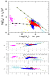 |
Fig. A.1. Ie-Re plane (top panel) and the 3DKS (bottom panel) for the MRR of Bernardi et al. (2010), Eq. 13. The agreement with observational data is not as good as it is with the Cosmic Galaxy Shepherd. |
The situation worsens further if we suppose that the MRR is the one suggested by Fan et al. (2010). If this MRR is in fine agreement with theoretical models of single galaxies born at different redshift and observed today, it is not able to match the observed distribution of galaxies in the Ie-Re plane and 3DKS. The effect of the halo mass function is missing here, while it is present instead in the Cosmic Galaxy Shepherd. The inadequacy of the Fan et al. (2010) MRR is demonstrated in Fig.A.2.
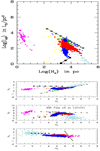 |
Fig. A.2. Ie-Re plane (top panel) and the 3DKS (bottom panel) for the MRR of Fan et al. (2010), Eq. 15. The adopted MRR is not compatible with the distribution of real galaxies in both panels. |
All Tables
MRRs derived from observational data and expressed as log Re = Alog Ms + B adopted in this study.
Estimates of the duration of star formation activity ΔTsfr and age of the last episode of star formation Tstars in objects of different stellar mass Ms.
All Figures
|
Fig. 1. 3DKS of the Burstein et al. (1997) data and the Illustris sample. The red dots are the ETGs, the green dots the LTGs, the coral dots the DGs, the magenta dots the GCs, the light-blue dots the GCGs, and the blue dots are the Illustris galaxies. To avoid overcrowding of the panels that data of Bernardi et al. (2010) and of the WINGS survey are not plotted. They overlap the Burstein et al. (1997) data. However, it is worth recalling that the observational data of Burstein et al. (1997) are in the B-band while the Illustris models are in the V-band. Consequently, there is a systematic offset among the two groups of data. Therefore, the comparison is only of qualitative nature. Nevertheless, the Illustris models overlap the LTGs, ETGs and a large part of the DGs, implying an acceptable agreement between theory and observations. |
| In the text | |
|
Fig. 2. Re-Ms plane of the observational data and theoretical models adopted in this study. Data: here, we show three sources of observational data and two types of MRRs. The samples of data are: (i) Burstein et al. (1997) for GCGs (light powder-blue dots), ETGs (red dots), DGs (blue dots) together with those by Geha et al. (2006) and Woo et al. (2008; green dots), and GCs (violet dots); (ii) The Bernardi et al. (2010) data for ETGs (dark red dots) together with their best fit (the long dashed line). These ETGs fully overlap those of Burstein et al. (1997); (iii) The WINGS data for GCGs (dark grey dots), BCGs (black dots), and ETGs (purple dots). Also in this case there is full coincidence with the corresponding objects of the previous samples. MRRs: the dark goldenrod thick solid line is the Cosmic Galaxy Shepherd of Chiosi et al. (2020) at redshift z = 0; this MRR folds together the galaxy MRR expected from cosmological HDF of halos. The solid orange lines are MRRs of Fan et al. (2010) for redshift zf = 0 (top), 1, and 5 (bottom). Models: theoretical hydrodynamic models of galaxies to be compared with observational data are (i) the Illustris galaxies (light green small dots) for z = 0 that are partially masked by the observational data of ETGs; (ii) the low initial density models (blue filled circles joined by their best-fit line) and the high initial density ones (red filled circled joined by their best-fit) by Chiosi & Carraro (2002); and (iii) the early hierarchical models by Merlin et al. (2012; black squares and their best-fit). See the text for more details. |
| In the text | |
|
Fig. 3. MB (top) and MV (bottom) magnitudes vs. age relationships for SSPs of different metallicities that are indicated by the color code. From the top to the bottom, the metallicies are Z = 0.0001, 0.001, 0.010, 0.019, 0.040, and 0.070. The black dotted lines are the mean values of MB and MV over the metallicity. |
| In the text | |
|
Fig. 4. Ie-Re plane and 3DKS of SSP galaxy models with with the MRR of Eq. (15), i.e., the Cosmic Galaxy Shepherd. The specific intensity Ie in use is for the B-passband. Left panel: the Ie-Re plane for the case with the constant ratio m = MDM/MS = 25, and the SFH described in the text. The black squares are the GLO-models while the dark olive green squares are the GAL-models. The small dots are the data of Burstein et al. (1997) and Illustris using the same color code of Fig. 1. In the same panel we also show GLO-models in which the ratio m = MDM/MS = 5. See the text for more details. Right panel: the corresponding 3DKS. Symbols and color codes are the same as in the left panel. The GLO-models for m = MDM/MS = 5 are not displayed because the difference with respect to those with m = MDM/Ms = 25 is very small. |
| In the text | |
|
Fig. 5. Same as in Fig. 4. Left panel: Ie-Re plane. Right panel: 3DKS. The physical assumptions for the SSP-models and meaning of the symbols are the same as in Fig. 4. The only difference here is that we adopt ratio MDM/Ms given by Eq. (18) to calculate the SSP-models. |
| In the text | |
|
Fig. 6. Same as in Fig. 4. Left panel: Ie-Re plane. Right panel: 3DKS. The physical assumptions for the SSP-models (the blue squares and solid lines) and meanings of the symbols are the same as in the previous figures. The ratio MDM/Ms is given by Eq. (18) and therefore varies with mass, MDM, and the MRR is that of the Cosmic Galaxy Shepherd. The only important difference is that both in the GLO and GAL models the radius predicted by the Cosmic Galaxy Shepherd is increased by a random quantity within the range indicated in Table 3 and Ie is accordingly decreased. In the left panel the results are plotted as a function of the reference radius to highlight the fact that the radius is changed at constant mass. The experiment is meant to show that the areas delimited by the GLO and GAL models can be populated by objects with a radius larger than the MRR of the Cosmic Galaxy Shepherd. All the models in the area comprised between the GLO and the GAL lines have no physical counterparts and should be discarded. The same considerations apply to the 3DKS shown in the right panel. |
| In the text | |
|
Fig. 7. Same as in Fig. 4. Left panel: Ie-Re plane. Right panel: 3DKS. The physical assumptions for the SSP-models and meaning of the symbols are the same as in Fig. 4. The only difference here is that the duration of the star formation activity ΔTsfr is supposed to always increase with the galaxy mass (solid black lines and black filled squares). This case strictly mimics the hierarchical scheme of galaxy formation. For sake of comparison, we also plot the curve for a constantly decreasing ΔTsfr (the green solid line and green filled squares). In the first case, while the upper border of the observational data on the Ie-Re plane is still reasonably matched (but for the most massive ETGs and galaxy clusters), serious difficulties occur with the 3DKS, in particular: with the k3 vs. k1 plane, where the distributions of ETGs and the FP are not fitted at all. |
| In the text | |
|
Fig. 8. Combined relationship for GLO and GAL models together. Left panel: Ie-Re plane in which the combined relation is shown against the observational data of Burstein et al. (1997). Right panel: corresponding 3DKS for the same models. In both panels, the meaning of the symbols is the same as in previous figures. No particular remarks are to be made here, aside from noting a general agreement between data and theory. The kind of SFH we have adopted seems to be compatible with the overall observational situation. |
| In the text | |
|
Fig. 9. Same as in Fig. 4. Left panel: Ie-Re plane of the model galaxies with infall. The mass MBM(TG) grows from left to right in steps of a factor of 10 from 106 to 1013 M⊙. The infall timescale, τ, and specific efficiency, ν, of star formation are listed in Table 5. The MRR relation is from Chiosi et al. (2020), the Cosmic Galaxy Shepherd. The blue lines are models with active star formation all over the evolutionary history. The red lines are models in which star formation is quenched off past the age t ≃ τ. The green and magenta lines indicate model with active (green) and quenched off (magenta) star formation, but in which the MRR relation for galaxies with stellar mass in the interval 106–109 M⊙ is that of the dwarf galaxies of Woo et al. (2008). See the text for more details. Right panel: Projections of the 3DKS. In each sub-panel, all the symbols have the same meaning as in the left panel. In each line the final stage (present age) is close to the observational data. It is worth noting that in the k3 vs. k1 plane the relation passing through all the final stages of the models with quenched star formation at the present age perfectly coincides with the FP plane of ETGs in the Virgo and Coma clusters. |
| In the text | |
|
Fig. 10. Evolution of the Illustris galaxies on the Ie-Re plane (left panel) and the 3DKS (right panel) from z = 4 to z = 0. There are four values of the redshift with the following color code: blue (z = 4.0), magenta (z = 2), green (z = 1), and red (z = 0). In the left panel, we also display the GLO and GAL lines of the reference case. The right panel is split in three parts showing the correlations k3 vs. k1 (top), k2 vs. k1 (middle), and k3 vs. k2 (bottom). In the k3 vs. k1 plane, which shows the fundamental plane, we also plot the relation derived by Burstein et al. (1997) for ETGs in the Virgo and Coma clusters (k3 = 0.15k1 + 0.36, dashed line) and the same for the Illustris objects falling in the region of ETGs of the MR plane (k3 = 0.20k1 − 0.075, solid line). The agreement is fairly good. In the middle diagram we also plot the ZOE line given by Burstein et al. (1997) with the equation: k2 + k1 = 8. |
| In the text | |
|
Fig. 11. 3DKS of ETGs (small red squares) and DGs (small green squares) of the Local Universe (hence, at the present age, z = 0) by Burstein et al. (1997). The data are compared with the monolithic models by Chiosi & Carraro (2002) for two formation redshifts and hence initial densities. The high initial density models (z ≃ 5) are indicated by the red triangles and the red dashed line, while the low density ones (z ≃ 1) by the blue squares and the blue dashed line. In all panels, the empty circle shows the position of M32 (NGC221). The solid black line in the k1 vs. k3 plane is the best fit of the models for ETGs, the slope of which nicely coincides with the slope of the FP for ETGs in Virgo and Coma clusters. The equations for the FP are k3 = 0.14k1 + 0.41 for the models and k3 = 0.15k1 + 0.36 for the real galaxies. The agreement if fairly good. In the background, we also show the Illustris models at z = 4 (light green dots). We note the striking difference of the galaxy distribution in the three planes at varying redshift. |
| In the text | |
|
Fig. 12. M/L vs. M projection of the FP in the SDSS r′-band, i.e. the relation log(Ms/Ls)⊙ = log(M/Lr′)⊙ vs. log Ms, where log Ms is the stellar mass enclosed within the half-light radius, in units of 1012 M⊙ and calculated according to Bell et al. (2003; left) and Gallazzi et al. (2005; right). Lr′ is the r′ luminosity enclosed within the half light radius. The small dots in both panels are the data from the catalog by Bernardi et al. (2010; priv. comm.), whose linear fit is shown as a continuous line. The big filled circles refer to our sets of models (12 models × 3 projection planes = 36 models) and the best fit of the intermediate and high mass models is shown as a dashed line. The dispersion of the models along the vertical axis, in particular for the high mass ones, is mainly due to their different initial conditions. |
| In the text | |
|
Fig. 13. Fundamental plane in the 3DKS for the SDSS g′ (left) and r′ (right) bands. In all the panels, the small dots are the elliptical galaxies of Bernardi et al. (2010). The meaning of the symbols is the same as in Fig. 12. |
| In the text | |
|
Fig. A.1. Ie-Re plane (top panel) and the 3DKS (bottom panel) for the MRR of Bernardi et al. (2010), Eq. 13. The agreement with observational data is not as good as it is with the Cosmic Galaxy Shepherd. |
| In the text | |
|
Fig. A.2. Ie-Re plane (top panel) and the 3DKS (bottom panel) for the MRR of Fan et al. (2010), Eq. 15. The adopted MRR is not compatible with the distribution of real galaxies in both panels. |
| In the text | |
Current usage metrics show cumulative count of Article Views (full-text article views including HTML views, PDF and ePub downloads, according to the available data) and Abstracts Views on Vision4Press platform.
Data correspond to usage on the plateform after 2015. The current usage metrics is available 48-96 hours after online publication and is updated daily on week days.
Initial download of the metrics may take a while.