| Issue |
A&A
Volume 694, February 2025
|
|
|---|---|---|
| Article Number | A229 | |
| Number of page(s) | 19 | |
| Section | Extragalactic astronomy | |
| DOI | https://doi.org/10.1051/0004-6361/202453201 | |
| Published online | 18 February 2025 | |
The role of dry mergers in shaping the scaling relations of galaxies
Department of Physics and Astronomy, University of Padua, Vicolo Osservatorio 3, I35122 Padua, Italy
⋆ Corresponding authors; This email address is being protected from spambots. You need JavaScript enabled to view it.
, This email address is being protected from spambots. You need JavaScript enabled to view it.
, This email address is being protected from spambots. You need JavaScript enabled to view it.
Received:
28
November
2024
Accepted:
16
January
2025
Abstract
Context. In the context of the hierarchical formation of galaxies, we investigated the role played by mergers in shaping the scaling relations of galaxies, that is the projections of their fundamental plane onto the Ie − Re, Ie − σ, Re − Ms, and L − σ planes. To this end, based on the scalar virial theorem, we developed a simple theory of multiple dry mergers to read both the large-scale simulations and the companion scaling relations.
Aims. The aim was to compare the results of this approach with the observational data and with two of the most recent and detailed numerical cosmo-hydro-dynamical simulations: Illustris-TNG and EAGLE (Evolution and Assembly of GaLaxies and their Environments).
Methods. We derived these scaling relations for the galaxies of the Mapping Nearby Galaxies at APO (MaNGA) and Wide-field Imaging of Nearby Galaxy-Clusters Survey (WINGS) databases and compared them with the observational data, the numerical simulations, and the results of our simple theory of dry mergers.
Results. The multiple dry merging mechanism is able to explain all the main characteristics of the observed scaling relations of galaxies, such as slopes, scatters, curvatures, and zones of exclusion. The distribution of galaxies in these planes is continuously changing across time because of the merging activity and other physical processes, such as star formation, quenching, and energy feedback.
Conclusions. The simple merger theory presented here yields the correct distribution of galaxies in the main scaling relations at all cosmic epochs. The precision is comparable with that obtained by the modern cosmo-hydro-dynamical simulations, with the advantage of providing a rapid exploratory response on the consequences engendered by different physical effects.
Key words: galaxies: evolution / galaxies: fundamental parameters / galaxies: general / galaxies: high-redshift / galaxies: structure
© The Authors 2025
 Open Access article, published by EDP Sciences, under the terms of the Creative Commons Attribution License (https://creativecommons.org/licenses/by/4.0), which permits unrestricted use, distribution, and reproduction in any medium, provided the original work is properly cited.
This article is published in open access under the Subscribe to Open model. This email address is being protected from spambots. You need JavaScript enabled to view it. to support open access publication.
1. Introduction
In recent years several studies have addressed the problems posed by the observed scaling relationships (ScRs) of galaxies. It is clear today that the information encrypted in the ScRs is of fundamental importance to understanding the physical processes that occurred during the evolution of galaxies. The formation, structure, and evolution of galaxies depend on several phenomena (e.g. mergers, stripping, star formation events, feedback) that in most cases leave imprints on the observed galaxies’ distribution in different ScRs. The analysis of the ScRs is therefore of great importance in order to reconstruct the history of galaxies and the evolution of our Universe.
Many physical parameters of galaxies are mutually correlated, in particular those defining the virial theorem (VT) and the fundamental plane (FP) (log(Re) = alog(σ)+blog(⟨I⟩e)+c). The mass correlates with the radius (Re − Ms), the luminosity with the velocity dispersion (L − σ), the effective surface brightness with the radius (Ie − Re), for example. In log units these relations are often linear, but significant deviations are visible in particular when the distributions of massive and dwarf galaxies are compared. In addition, when the sample of galaxies includes objects of very different luminosities, the ScR variations of the mean slopes and zones of exclusion (regions empty of galaxies) are visible.
To date, most of the efforts of the astronomical community have been dedicated to the analysis of the peculiar characteristics of each ScR. For example, many studies address the problem posed by the slope, zero-point, curvature, and scatter (among many others; see e.g. Oegerle & Hoessel 1991; Bernardi et al. 2003; Shen et al. 2003; Courteau et al. 2007; Desroches et al. 2007; Sanders 2010; Nigoche-Netro et al. 2011; Hyde & Bernardi 2009; Montero-Dorta et al. 2016; Samir et al. 2020; D’Onofrio et al. 2024; Quenneville et al. 2024). Other studies highlight the role played by the environment, feedback effects, dissipation, mergers, dark matter halos, galaxy morphology, and dynamics, and by cosmology (see e.g. Bender et al. 1992; Burstein et al. 1995; Chiosi & Carraro 2002; Boylan-Kolchin et al. 2006; Damjanov et al. 2009; Fan et al. 2010; Bernardi et al. 2011; Shankar et al. 2013; Agertz & Kravtsov 2015; Krajnović et al. 2018; Sánchez Almeida 2020; Chiosi et al. 2023). A different approach, followed by many researchers, is that of comparing the results of numerical simulations with the observed galaxies in various ScRs (see e.g. Lange et al. 2016; Ferrero et al. 2017; Furlong et al. 2017; Pillepich et al. 2018a,b; Genel et al. 2018; Huertas-Company et al. 2019; Cannarozzo et al. 2023).
The approach followed here is somewhat different from the previous ones, and finds its roots in a series of papers (D’Onofrio et al. 2017; D’Onofrio et al. 2019; D’Onofrio et al. 2020; D’Onofrio & Chiosi 2021; D’Onofrio & Chiosi 2022; D’Onofrio & Chiosi 2023a; D’Onofrio & Chiosi 2023b) that are based on the assumption that instead of separately analysing the single ScRs, more significant information can be extracted by simultaneously looking in a self-consistent way at all the mutually related ScRs. The novelty of this approach is to look at the behaviour of each galaxy during its evolution, taking into account that both luminosity and mass (and consequently all the other related parameters) continuously change for many reasons (e.g. star formation, mass acquisition and depletion by mergers or stripping events, natural aging of their stellar populations).
In the paradigmatic hierarchical context, repeated mergers among galaxies occur and change the properties of these latter. At each merger, the dynamical structure and equilibrium of a galaxy is perturbed, while for most of the remaining time the galaxy is in mechanical equilibrium, that is they obey the VT. Based on these grounds, D’Onofrio et al. (2017) first generalized the luminosity–velocity dispersion relation by explicitly introducing the time dependence. The new relationship is
where t is the time and σ the velocity dispersion. The proportionality coefficient L′0 and the exponent β are functions of time and can vary from galaxy to galaxy. Then, by coupling this law with the VT, which is a function of Ms, Re, and σ, they obtained a system of equations in the unknowns log L′0 and β whose coefficients are functions of the variables characterizing a galaxy (Ms, Re, L, σ, and Ie).
The new empirical relation, although formally equivalent to the Faber–Jackson (FJ) relation for early-type galaxies (ETGs) (Faber & Jackson 1976), has a profoundly different physical meaning: β and L′0 are time-dependent parameters that can vary considerably from galaxy to galaxy, according to the mass assembly history and the evolution of the stellar content of each object. These parameters are found to be good indicators of a galaxy’s mass accretion history, star formation, and evolutionary processes, and offer an immediate insight into its current stage of evolution. The β parameter determines the direction of motion of a galaxy in the space of parameters at the base of the VT.
Adopting this new perspective, it was possible to simultaneously explain the tilt of the FP and the observed distributions of galaxies in the FP projections and, at the same time, to understand the real nature of the FJ relation. Then, having demonstrated that the ScRs observed today originate from the motion in the parameter space of each individual galaxy during its evolution, what is still lacking is to understand which physical phenomena drive the change of shape of the ScRs in the course of time. In order to reach this goal we proceeded here in two parallel ways: (i) First, we compared the ScRs related to the VT (the Ie − Re, Ms − Re, and L − σ relations) with the most recent simulations of model galaxies in cosmological context, such as Illustris-TNG (Vogelsberger et al. 2014a,b) and EAGLE (Evolution and Assembly of GaLaxies and their Environments) (Schaye et al. 2015; McAlpine et al. 2016). The comparison was extended to z ∼ 1 where observations are currently available in sufficient number to allow a meaningful analysis, and to even higher redshifts to see what the simulations would predict. (ii) Then, to cast light on the effects of mergers in which different masses and energies are involved, on the various ScRs, we set up and present here a simple analytical model of mergers able to mimic the results of the large-scale simulations and to predict the path of galaxies in the parameter space in the course of time. This approach is based on the idea that galaxies in isolation are in virial equilibrium, and that a merger is a perturbation of this state of short duration so that a new equilibrium condition is soon recovered. On these grounds, the formation and evolution of a galaxy can be conceived of as an isolated object whose mass and radius from time to time are increased by a merger likely causing additional star formation.
Starting from the idea and the formalism developed by Naab et al. (2009) about the material falling on an already formed object during a single merger, we generalized their formalism to the case of a series of successive dry mergers among galaxies of different masses. We show that this simple idea is able to catch the observed distribution of galaxies in the ScRs, making the dry merging phenomenon the principal mechanism shaping the ScRs observed today. We also show that this approach is consistent with the results obtained in our previous studies (see e.g. D’Onofrio et al. 2017; D’Onofrio et al. 2020; D’Onofrio & Chiosi 2021; D’Onofrio & Chiosi 2022; D’Onofrio & Chiosi 2023b). The advantage, with respect to the sophisticated numerical simulations, is in the possibility of obtaining new results on a short timescale and at no cost, whenever one may want to explore different solutions, such as different initial conditions, different efficiencies of mergers, and different laws and modes of star formation.
The paper is structured as follows. Section 2 presents the observational databases used for our comparisons of the structural parameters with the predictions of theoretical models. Section 3 introduces the EAGLE and Illustris-TNG simulations used in our analysis of the ScRs. Section 4 shows the comparison of simulations with the observational data at z ∼ 0. Section 5 gives an idea of the predicted distribution of galaxies in the ScRs at high redshift according to simulations. Section 6 presents the mean behaviour of galaxies across time predicted by extensive numerical simulations. Section 7 is dedicated to presenting our simple analytical model of dry galaxy mergers, and to a quick comparison with the observational data and the model galaxies produced by numerical simulations. In Sect. 8 we compare the observational data with the hydro-dynamical simulations. Section 9 contains a detailed comparison of the results obtained from our analytical models and the observational data and hydro-dynamical simulations. Section 10 summarizes the β − L0′ theory of D’Onofrio & Chiosi (2024, and references therein) and compares the results derived from the application of it to the analytical model and observational data. Finally, in Sect. 11 we draw our conclusions.
2. The observational data
Three galaxy samples were used for this work. The first is the same adopted in our previous studies on the subject (see D’Onofrio & Chiosi 2022; D’Onofrio & Chiosi 2023a), that is the data at redshift z ∼ 0 taken from the Wide-field Imaging of Nearby Galaxy-Clusters Survey (WINGS) and Omega-WINGS databases (Fasano et al. 2006; Varela et al. 2009; Cava et al. 2009; Valentinuzzi et al. 2009; Moretti et al. 2014, 2017; D’Onofrio et al. 2014; Gullieuszik et al. 2015; Cariddi et al. 2018; Biviano et al. 2017). The whole WINGS photometric sample contains more than 32 000 galaxies of all morphological types. The sub-sample also used here contains only ETGs, generally with stellar mass Ms > 109 M⊙. It has 270 galaxies, with measurements of their stellar masses, star formation rates (measured by Fritz et al. 2007), morphologies (given by MORPHOT; Fasano et al. 2012), effective radii and total luminosities measured by GASPHOT (Pignatelli et al. 2006; D’Onofrio et al. 2014) and velocity dispersions, collected from the literature.
The second galaxy sample is that of MaNGA (Mapping Nearby Galaxies at APO) survey (Smee et al. 2013; Bundy et al. 2015; Drory et al. 2015; Blanton et al. 2017). MaNGA obtained spectral and photometric measurements of nearby galaxies of different morphological types (∼10 000 objects across ∼2700 sky square degree), thanks to the “integral field units” (IFUs) of the Apache Point Observatory (APO). MaNGA is a byproduct of the SDSS survey and was designed to study the history of present day galaxies.
MaNGA has provided many galaxy parameters, including morphology, stellar rotation velocity and velocity dispersion, magnitudes and radii, mean stellar ages and star formation histories, stellar metallicity, element abundance ratios, stellar mass surface density, ionized gas velocity, star formation rate, and dust extinction. The galaxies were selected to span a stellar mass interval of nearly three orders of magnitude and no selection was made on size, inclination, morphology and environment, so this sample is fully representative of the local galaxy population and can be compared with the modern hydro-dynamical simulations such as EAGLE and Illustris-TNG, which, however, do not provide information on the morphological types of their model galaxies. The present sample contains information for 10 220 galaxies of all morphological types.
To get a qualitative idea of the ScRs we would expect from the two datasets we present here the Ie − Re plane as an example (Fig. 1). ETGs and LTGs are in general well mixed in this plot, but for the ETGs which in general have larger radii Re. The two datasets nicely overlap, with the exception of the largest ETGs that are not observed in MaNGA. Probably this is due to the fact that WINGS includes galaxies in clusters containing a number of very bright objects.
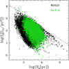 |
Fig. 1. Comparison of the Ie − Re plane for the WINGS and MaNGA data. The black symbols mark the whole WINGS dataset, while the green symbols indicate the MaNGA data. All morphological types are included for both datasets. |
At higher redshift (z ∼ 1), the third sample in use is the Large Early Galaxy Astrophysics Census (LEGA-C) database. This sample contains ∼4000 galaxies with measured parameters for objects at z > 0.6 (van der Wel et al. 2021). Details on these measurements can be found in the cited paper and references therein.
In the general, the parameters L, Ms, Re, σ, Ie are surely affected by some uncertainty, which for each object is estimated to amount to about 10 to 20% at maximum. Since we are always using variables in logarithmic scale, uncertainties of this entity would correspond error bars from 2 × 0.042 to 2 × 0.079. Therefore, when presenting large samples of data with parametes encompassing wide intervals, error bars of this length would simply add some small noise to the general trends. For this reason, the data are always plotted neglecting the errors bars.
3. The EAGLE and Illustris-TNG data
The simulations of galaxy formation and evolution used here are EAGLE and Illustris-TNG.
EAGLE (Schaye et al. 2015; McAlpine et al. 2016) is a large-scale hydro-dynamical simulation of the Lambda-Cold Dark Matter universe (Λ-CDM). The project aims at examining the formation of galaxies and the co-evolution with the gaseous environment. In this simulation, great care was put in the treatment of feedback from massive stars and in the presence of accreting black holes. EAGLE provides many galaxy parameters. Those used here are the galaxy mass and luminosity, the mean effective half mass radius, the mean velocity dispersion of the star particles and the star formation rate.
Illustris-TNG (Springel et al. 2018; Nelson et al. 2018; Pillepich et al. 2018b) is the new version of Illustris-1. The new simulation seems to produce results in better agreement with the observations (Nelson et al. 2018; Rodriguez-Gomez et al. 2019). In Illustris-TNG the structural parameters of galaxies, such as colours, magnitudes and radii, are in quite good agreement with the available data at low redshift (Rodriguez-Gomez et al. 2019). Here we used the TNG100 dataset. The extracted structural parameters are the same as the EAGLE one.
For both EAGLE and TNG100 simulations, the main progenitor branches of the merger trees were considered to follow the evolution of the same objects along time. The more massive galaxy has been always selected as the progenitor of each object going back to high redshift, from z = 0 to z = 4, in steps of 1.
Only those object that were already formed at z = 4, with a stellar mass higher than the mass resolution of the simulations (Mres = 1.4 × 10⁶ M⊙) at all redshifts, and have a stellar mass Ms > 108.5 at z = 0, were considered. To have datasets that are easier to handle and at the same time to keep the statistical robustness, only a maximum of 150 objects for each 0.2 dex of stellar mass at z = 0 were considered. At the end, a total of 2400 and 2200 objects were taken into consideration for EAGLE and TNG100 simulations, respectively.
With these data we want to demonstrate that (i) these two hydro-dynamical simulations reproduce quite well the main characteristics of the observed ScRs at z = 0; (ii) our simple mathematical models of galaxy structure are good proxies of both observational data and numerical N-body hydro-dynamical simulations.
4. The ScRs at low redshift
Figure 2 shows the Ie − Re plane of the MaNGA database with superposed the results of the EAGLE (left panel) and Illustris-TNG100 (right panel) simulations. It should be remarked that the half light radius provided by the MaNGA data is somewhat different from the half mass radius given by simulations. Nevertheless, it is clear that both simulations reproduce many of the features observed in the Ie − Re plane. This is the case, for example, of the Λ-shaped distribution of galaxies observed in this plane, in which the more massive galaxies are distributed along a tail with a slope ∼ − 1, while the dwarf galaxies spread out on a cloud that extends along the vertical direction. In our plot all morphological types are shown for both the observational data and simulations. In the case of the MaNGA data, the addition of the spiral galaxies produces a more uniform distribution of galaxies in the Ie − Re plane in which the Λ-shape is less visible.
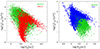 |
Fig. 2. Comparison of the Ie − Re plane with the MaNGA data and simulations: EAGLE in the left panel and TNG100 in the right panel. The green crosses mark the MaNGA data for all morphological types, while the red circles are for the EAGLE data and the blue circles are for TNG100. |
We note that the EAGLE radii are systematically larger than the TNG ones. This produces the higher surface brightness observed for the TNG data.
The lack of objects at low radii and very low surface brightness, that appears as a boundary, is due to selection effects. Only galaxies above a given luminosity are present in the observational data as well as in simulations.
On top right, we remark the presence of the Zone of Exclusion (ZoE). This boundary has a slope close to −1, a value predicted by the VT. No galaxies reside beyond this limit (at least at z = 0, the present time). The origin of this boundary is still a matter of debate (see e.g. Bender et al. 1992; Secco 2001; D’Onofrio et al. 2006).
Figure 3 shows the Re − Ms plane for the same data-sets. Here again simulations are able to reproduce the curvature of the distribution at the high masses and the zone of exclusion on the right side with slope ∼1. Only the scatter in radius is not fully matched. The observational data gives a much larger distribution of Re. As for the previous plot this occurs when the spiral galaxies are added to the distribution.
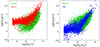 |
Fig. 3. Comparison of the Re − Ms plane with the MaNGA data and simulations. In the left panel the EAGLE models, in the right panel the TNG100 models. The colour-coding and symbols are as before. |
In this plot it is better visible the systematic difference in the half-mass radius between EAGLE and TNG100. It is beyond the aims of this study to analyse in detail why this occurs. We limit ourselves to noting that the physical prescriptions used in the two simulations give rise to systematically different radii (most likely due to feedback effects).
The simulations also predict radii of the low mass galaxies (those with Ms < 109 M⊙) that are not present in our observational database. The flattening of the distribution at low mass galaxies is clearly visible both in the observational data and theoretical simulations. In contrast, the tail formed by the massive galaxies is well matched by the models.
Fig. 4 shows the L − σ plane. It is clear that in this case both sets of simulations do not fully reproduce the slope and the scatter in luminosity at each value of the velocity dispersion σ. A number of explanations can be found for this. It should be recalled for example that the MaNGA data derives σ from the IFU. It follows that the velocity dispersion depends on the aperture of the fiber elements with respect to the galaxy dimension and the orientation of the galaxy. On the theoretical side, simulations provide the mean velocity dispersion of the star particles within the half mass radius. The two measurements are far from being identical. Despite this, a clear correlation of the two parameters is evident for both data samples.
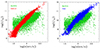 |
Fig. 4. Comparison of the L − σ plane with MaNGA data and simulations. In the left panel the EAGLE models, in the right panel the TNG100 models. The colour-coding and symbols are as before. |
The slope of the theoretical relation is slightly higher with respect to that of the data. Observations indicate that the galaxies of low luminosity progressively depart from the L − σ relation and are distributed along a horizontal cloud of points. On the other hand, simulations predict a L − σ relation holding over the whole range of magnitudes with nearly constant scatter everywhere. Clearly the MaNGA data indicates that the addition of the spiral galaxies in this diagram, originally drawn only for pressure-supported systems such as E and S0 galaxies, yields a less sharp and scattered distribution. The question arises, why simulations of all types of objects, yield such a narrow distribution. Probably, this is due to the definition of velocity dispersion made for these systems.
As a final remark, we note that the model galaxies predict a slightly curved distribution that is not visible in the observational data. It is not the aim of this work to discuss the possible explanations for the observed differences between observations and simulations. The qualitative comparison made here wants only to demonstrate that the present hydro-dynamical simulations are able to reproduce many of the main features of the observed distributions in all the ScRs generated by the FP projections. Examining these issues in more detail is left to other studies, more focused on understanding the limits and drawbacks affecting the present-day simulations of galaxies.
In other words, the physical prescriptions adopted in the theoretical models catch the main behaviour of galaxies in all ScRs. Perfect overlapping is, however, still lacking and requires some more work on several basic parameters that define a galaxy, for example a better description of the luminosity profile at base of the half-mass core and half-mass radius and differences from galaxy to galaxy.
5. Going up towards high redshift
At z ∼ 1 the sample of galaxies provided by the LEGA-C survey contains only the brightest objects. Fig. 5 shows the comparison with the TNG100 data at the same redshift. The comparison with EAGLE is very similar and we decided not to plot it here. Again both simulations catch the main features of the ScRs. However, the L − σ relation is only partially reproduced. Observations seem to indicate a much flatter distribution with respect to simulations. The reasons are likely the same as before. The data gives only the central velocity dispersion while the simulations yield the mean value of it inside the half-mass radius. In addition, a number of problems surely affect the measurement of σ at high redshifts. Nevertheless, the bulk of the distribution for the massive model galaxies well agrees with the observational data.
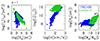 |
Fig. 5. Comparison of the Ie − Re, L − σ, and Re − Ms planes for the LEGA-C data (green dots) and the TNG100 simulations (blue dots). The data and models refer to galaxies observed and/or predicted at redshift z = 1. |
On the basis of the comparison of the structural parameters at z = 0 and z ∼ 1, we may argue that the results of theoretical simulations provide a quite good descriptions of reality and therefore we can proceed to examine what they would predict for the ScRs at higher redshifts.
Figs. 6 and 7 show the predictions of EAGLE and Illustris-TNG for the ScRs at different redshifts, from z = 1 to z = 4. There is a substantial agreement between the two samples of models. Both predict that the effective half-mass radius decreases at high redshift, in particular that of massive galaxies. Consequently, the surface brightness increases together with the luminosity and the tails in the Ie − Re and Re − Ms planes disappear.
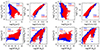 |
Fig. 6. Comparison between EAGLE (red dots) and TNG (blue dots) at z = 1 (the group of four panels at the left) and z = 2 (the group of four panels at the right) in four ScRs: the Ie − Re plane (top left), the Ie − σ plane (top right), the Re − Ms plane (bottom left), and the SFR–Ms plane (bottom right). |
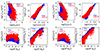 |
Fig. 7. Comparison between EAGLE and TNG at z = 3 (left panel) and z = 4 (right panel). The symbols and diagrams are as in Fig. 6. |
At high redshift both simulations predict a Re − Ms relation curved towards an opposite direction with respect to that observed at z = 0: massive galaxies are all very small in size and bright in luminosity.
The relation between the star formation rate (SFR) and the mass of galaxies is very similar, with the number of objects in the phase of SF quenching and/or already quiescent, that increases going towards the present epoch.
The L − σ relation is progressively less curved going up in redshift and the scatter remains always approximately the same.
6. The mean evolutionary path of galaxies in simulations
Figs. 8 and 9 give an idea of the mean evolutionary change in the structural parameters experienced by galaxies of different masses up to the present time (z = 0). Objects with present mass larger than 1011 M⊙ and those with masses lower than 109 M⊙ are shown in the figures with different colours. Fig. 8 refers to the EAGLE simulation, while Fig. 9 to TNG100. Both simulations show that the massive galaxies increase in radius with time, while the low massive objects essentially maintain the same radius. The mass increases with time, approximately with the same rate. The surface brightness decreases, in particular for the more massive galaxies. The same is true for the SFR, that decreases towards the present epoch. The total luminosity first increases and then starts to decrease. The M/L ratio always increases towards the present time. The stellar velocity dispersion increases for the massive galaxies while it remains approximately the same for the low mass objects. The parameter β defined by D’Onofrio & Chiosi (2021, see also below) presents a large scatter around zero for the massive galaxies, while it remains always close to zero for the less massive ones.
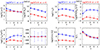 |
Fig. 8. Mean evolutionary path of galaxies in the EAGLE simulations. The blue dots and lines give the mean path of the galaxies with current masses higher than 1011 M⊙, while the red dots and lines those for the masses lower than 109 M⊙. The variables Re, Ms, Ie, and β are plotted against the redshift z. |
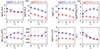 |
Fig. 9. Mean evolutionary path of galaxies in the TNG simulations. The colours, symbols, and diagrams are as in Fig. 8. |
The galaxies that today have masses within the limits we have considered exhibit properties intermediate in between those we have described depending on their mass.
The galaxy parameters that undergo the largest variations across time are the half-mass radius and the SFR. We show, with the aid simple models of mergers, that this is due to the combined effects of dry mergers and quenching of the stellar populations.
7. The role of mergers in shaping the ScRs of galaxies: a simple model of dry mergers
In the first part of the paper, we compare the observational data to theoretical models calculated in the hierarchical scenario in which mergers among galaxies are the paradigm of their formation and evolution. Since data and theory were in satisfactory agreement, we have implicitly assumed that the hierarchical view was the right frame to work with and neglected to explore and highlight the role played by the merger mechanism in shaping the various scaling relations followed by galaxies. It goes without saying that the large-scale simulations of galaxy formation and evolution in cosmological context are so heavy to plan, perform, and interpret that changing the physical ingredients to explore their effect on the ScRs of galaxies is out of reach. So trying to develop a simple analytical model of mergers as a smart proxy of the large-scale numerical simulations is a meaningful and hopefully rewarding effort.
In this section we present a simple analytical model able to describe and predict the growth in radius as a consequence of the growth in mass by mergers together with the variations in luminosity, surface brightness, and velocity dispersion.
The model strictly stands on the formalism developed by Naab et al. (2009) for the case of a single object in virial equilibrium on which other objects of assigned total mass and energies fall in and merge together. Assuming energy conservation, the new system is also supposed to reach the virial equilibrium. The model we propose generalizes the formalism to the situation in which many successive mergers can occur. In addition to mass and radius the new model also considers the variations in luminosity and specific intensity.
The Naab et al. (2009) case. Let us start with the initial system characterized by mass Mi, half-mass radius Re, i, velocity dispersion σi, luminosity Li, specific intensity Ie, i. The kinetic (Ki), gravitational (Wi), and total (Ei) energies of the initial object are
The virial equilibrium is expressed by 2Ki + Wi = 0 from which one derives the two identities
We suppose now that the system i merges with another system a with parameters Ma, Ra, i, σa, La, Ia, i, Ka, Wa, and Ea, and that the virial condition is rapidly re-obtained after the merging. Finally, introduce the ratios η = Ma/Mi and ϵ = σa2/σi2. The total energy of the system is now Ef = Ei + Ea. After the merger event, the composite system soon recovers the virial equilibrium so that we can write
 (1)
(1)
where Mf = Mi + Ma = (1 + η)Mi. It follows from it that
 (2)
(2)
 (3)
(3)
 (4)
(4)
 (5)
(5)
Depending on the parameters η and ϵ the increase of the radius is different. If the mass is simply doubled Mf = 2Mi, η = 1 and hence ϵ = 1, the radius Re, f = 2Re, i, and the velocity dispersion σf = σi.
Extension to several mergers. The formalism can be easily extended to the case of many successive different mergers. For the sake of simplicity, we start considering an initial object characterized by the parameters Mi, Re, i, σi, Li, Ie, i in suitable units and capturing other objects characterized by the parameters Ma, Re, a, σa, La and Ie, a in the same units. In this step of the reasoning, the luminosity and specific intensity are not included. The number of mergers is given by N (integer). The captured objects are all the same and are small compared to the initial object. Define also the ratios η = Ma/Mi and ϵ = σa2/σi2. The final total mass is Mf = Mi + NMa. The initial galaxy, the captured object, and the final object are all in virial equilibrium. Following the reasoning of the two-body case, we arrive at the expressions
 (6)
(6)
 (7)
(7)
and the following scaling laws for the mass Mf, σf2, Re, f, and ρf as functions of the corresponding values of the initial galaxy
 (8)
(8)
 (9)
(9)
 (10)
(10)
 (11)
(11)
Luminosity and specific intensity. To include in the scaling laws those for the luminosity and specific intensity and derive the total luminosity Lf and the total specific intensity Ie, f of the remnant galaxy, we need to check in advance some preliminary aspects concerning the luminosity because of its complex nature, more complex than the case of the mass, radius, and velocity dispersion. Also in this case, the luminosity Li and specific intensity Ie, i of the initial object are taken as the reference values for the luminosity, La, and specific intensity Ie, a of the captured objects.
We start from the notion that the luminosity of a galaxy is proportional to its stellar mass content, the intensity of star formation, and the natural time evolution of its stellar populations. Looking at the luminosity to mass ratio L/M, the elementary theory of stellar population and many simple infall-models in literature (see for instance Tantalo 2005; Chiosi et al. 2023; D’Onofrio & Chiosi 2023b; D’Onofrio & Chiosi 2022, and references therein) show that at the beginning the ratio M/L is low (the effect of the luminosity overwhelms that of the mass), then grows to some value in relation to the star formation activity, and past the initial period dominated by star formation the ratio steadily increases with the age. The typical behaviour of the L/Ms and Ms/L ratios as function of the age and of the L/Ms ratio as function of the stellar mass Ms in infall models is shown in the left and right panels of Fig. 10, respectively. In the top panel, we also compare the L/Ms ratio to that of single stellar populations (SSPs) of suitable chemical composition (solar abundances in our case) and derive their best-fit lines. Galaxy models and SSPs have the same trend. In the bottom panel we compare the L/Ms variations as a function of the stellar mass of two model galaxies (106 M⊙ and 1012 M⊙). The two curves are identical but shifted by a certain factor (the mass). The best fit of the relations yields
 (12)
(12)
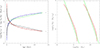 |
Fig. 10. Mass-to-luminosity and luminosity-to-mass ratios as functions of the age (left panel) and the luminosity-to-mass ratio as a function of the stellar mass Ms (right panel). The masses and luminosities are in solar units, the age is in Gyr. Left panel: In the panel the solid red and blue lines are the Ms/LV and Lv/Ms ratios, respectively, for an infall model of asymptotic mass of 1010 M⊙ calculated by the authors (see Chiosi et al. 2023, and references), while the black dots along each line are the same, but for a SSP with solar chemical composition taken from the Padova library (Tantalo 2005). The straight lines are the best fit of the relations. Right panel: Ms/LV ratio for two infall models with different masses. For each case the stellar mass increases along each curve from left to right. The two straight lines are the best fit of the data (see text for more details). |
where KMs is 7.43 for the 1012 M⊙ galaxy and 3.43 for the (106 M⊙) one. The intercept of the best-fit line is a function of the mass. Performing a linear interpolation and replacing the factor KMs, we obtain
 (13)
(13)
and
 (14)
(14)
The factor −0.57 can always be expressed as the logarithm of a suitable number −0.57 = Log A. Therefore we may write

where A ≃ 1/4. Consequently, in the derivation of the ratio Lf/Li the factor A will cancel out.
At this point we may wish to include also the effect of age on the luminosity emitted by the stellar populations of a galaxy. From the relations shown in the top panel of Fig. 10, but for a short initial period, the luminosity of a single galaxy tends to always decrease as a function of time. Furthermore, looking at the captured objects of a certain mass there is no reason to say that they all have the same age and in turn the same luminosity. We may cope with this by introducing in the mass luminosity relation a factor δ varying from galaxy to galaxy within a certain range (L = δAMs). Therefore, δ is related to the luminosity per unit mass and is also a function of time.
With the present formalism, it is convenient to normalize the luminosity of the generic captured object to that of the initial galaxy and write
 (15)
(15)
posing θj = δj/δi, we derive
 (16)
(16)
Since δj is an arbitrary quantity and Li is assigned, we may always pose δi = 1.
If η and θ are always the same we may write
 (17)
(17)
otherwise the summation is needed.
If one is not interested to highlight the time dependence of the luminosity variation, the factor θ can be neglected by simply posing θ = 1.
Since the specific intensity is given by Ie = L/(2πRe2), the associated scaling relation is
 (18)
(18)
The last two relations complete the systems of equations from (2) to (5) and from (8) to (11).
Before proceeding further, we present in Table 1 a few cases to illustrate the kind of effects we would expect on an initial object (Mi, Re, i, σi2 and Li) after a series of mergers with an object with Ma, Re, a, σa, and La) (always the same for simplicity). In the table masses are in M⊙, luminosities in L⊙, radii in kpc, and specific intensities in l⊙/pc2. The parameters η, ϵ, and θ are supposed to be constant.
Results from the analytical model of mergers.
Including the kinetic energy of the merging object. For the sake of investigation, we also took into account that the captured object with mass Ma, velocity dispersion σa, also carries the kinetic energy of the relative motion Ka = (1/2)Mava2. Part of this energy is supposed to be absorbed by the receiving object and the rest be dissipated in some way. Also in this case, the mass Ma and velocity va2 are parameterized in terms of the initial mass Mi and initial velocity dispersion σi by the relation Ma = ηMi and va2 = λσi2. After the merger, the composite system recovers the virial condition. With the aid of some simple algebraic manipulations, we obtain
 (19)
(19)
 (20)
(20)
 (21)
(21)
 (22)
(22)
 (23)
(23)
 (24)
(24)
We note that for λ = 0 the previous case is recovered.
Random variations of η, ϵ, λ, and θ. These relations can be further generalized to take into account the possibility that the parameters η, ϵ, λ, and θ can slightly vary from one galaxy to another and the merger event. The system of equations from Eqs. (19)–(24) becomes
 (25)
(25)
 (26)
(26)
 (27)
(27)
 (28)
(28)
 (29)
(29)
 (30)
(30)
where the suffix j goes from 1 to N. In the summations ∑jηj, ∑jϵj, ∑jηjϵj, ∑ηjλj, ∑ηjθj the parameters ηj, ϵj, λj, and θj are randomly varied within suitable intervals by means of uniform distribution of random numbers between 0 and 1. Also in this case for λj = 0 and θ = 1 we recover the standard cases with no kinetic energy of the relative motion and no age effect on the luminosity. When considering the effect of random variations on the key parameters η, ϵ, λ, and θ for each choice of the starting object we repeat the whole sequence a number of times (typically 10) and retain all the results. In the following the models based on this formalism are referred to as Mod-A.
Changing the reference model step by step. Before concluding this section, we would like to present an alternative formulation of the problem which differs from the previous one from the initial hypothesis and yet leads to similar results. In the previous version the key hypothesis was: an initial object of mass Mi that in all successive steps acquires a smaller object with the same mass Ma, and energy smaller that those of the initial object. The mass Mi and velocity dispersion σi are always the reference values.
In alternative we may suppose that at each merger the newly formed object becomes the reference system for the next episode. In other words, each merger is a two-galaxies event in which the parameters η, ϵ (and λ and θ) are referred to the last composed object. These parameters must be continuously adjusted step by step to keep the perturbation small compared to the current object. This is achieved by simply dividing the parameters η, ϵ, and λ by the current number of the step. The equations governing these models are
 (31)
(31)
 (32)
(32)
 (33)
(33)
 (34)
(34)
 (35)
(35)
 (36)
(36)
Given an initial set of values for Ms, Re, σ, L, Ie, a sequence of mergers at increasing mass is made by N steps indicated by J = 1, …N. In order to keep the perturbation small compared to the ever increasing mass we adopt the heuristic prescription η = ηr/J, ϵ = ϵr/J, θ = θr/Jλ = λr/J, where ηr, ϵr, λr, and θr are the usual factors, randomly varied within suitable intervals. Models of this type are named Mod-B.
Flowchart of the models and technicalities. Starting from the Naab et al. (2009) idea and formalism, Eqs. (2)–(5), we generalized it to the case of many mergers indicated by the parameter N, which can be any integer number from 1 to say 1000. This case is given by Eqs. (8)–(11). The choice of N is completely free, however some hint can be given by the ratio Mf/Mi between the final mass we want to reach and the initial mass we started with. The parameters η and ϵ are free but confined inside a suitable interval. To follow the gradual variation of the galaxy properties we retain a number of intermediate models from N = 1 to N = Nmax, sometime we refer to these models as a “sequence”.
Following the same line of thought we derived the relation for Lf/Li and Ie, f/Ie, i. These equations can be added to Eqs. (2)–(5) to complete them with the expected variations of luminosity and specific intensity, Eqs. (8)–(11).
Another important step is made by including the effect of the kinetic energy carried by the merging object (parameter λ). This case corresponds to Eqs. (19)–(24).
Finally, we suppose that the parameters η, ϵ, λ and θ instead of being rigorously constant passing from one model to another, they may suffer random fluctuations within some reasonable intervals of values. The new situation corresponds to Eqs. (25)–(30). This is the most general case.
All these models share the same basic feature, that is the merging object is always described in terms of the first merger of the whole sequence. This is true for the mass and the energy, for example. This type of model has been named Mod-A.
A completely different point of view has been adopted for the last group of models, named Mod-B and given by Eqs. (31)–(36). In this case the initial model model is varied along the sequence. In other words, we start with an initial galaxy characterized by the variables Mi, Ri, and σi, among others, on which another galaxy characterized by M = ηMi, σ = ϵσi, among others, can merge. The step corresponds to N = 1. The resulting object, with Mf, σf becomes the initial model for each successive step until a certain value of the mass or a maximum number of mergers has been reached. Along the sequence the parameters η, ϵ, λ, and θ are suitably decreased so that the merging object is a small perturbation compared to the existing one. The parameters η, ϵ, λ, and θ are also randomly varied within some suitable intervals passing from one step to the next. These models are the closed analytical simulation of real mergers.
8. Results from the analytical merger models
In this section we present some results of the analytical model of mergers with the aim of testing their ability to approximate the data of real galaxies and/or the results of detailed numerical simulations. We focus on three basic planes that can be set up with the physical quantities L, Ms, Re, σ, and Ie: the planes in question are Ie − Re, L − σ, and Re − Ms. The analysis is carried out using both Mod-A and Mod-B.
The first step of the procedure is to set the initial seed from which a sequence of mergers is simulated. To this aim, we consider four models of galaxies whose evolution is calculated according to the infall formalism of Tantalo et al. (1998). They are labeled according to the baryonic asymptotic mass MG = 106 M⊙, 108 M⊙, 1010 M⊙, and 1012 M⊙, that is the baryonic mass reached at the present time. The mass accretion time scale is τ = 1 Gyr. All other details of the models can be found in Chiosi et al. (2023). Suffice to recall here that they are supposed to start their evolution at redshift zf = 5 in the Λ-CDM Universe with parameters H0 = 71 km s−1 Mpc−1, Ωm = 0.27, and ΩΛ = 0.73 age of the universe Tu = 13.67 Gyr, age of the Universe at zf = 5 Tf = 1.2 Gyr, age of the galaxies at z = 0 TG = 12.47. For each sequence we mark six values of the redshift (4, 3, 2, 1, 0.5, and 0) at which the data for Ms, Re, σ, LV, Ie and M/L are recorded. They are the seeds of six sequences of merger simulations. All data are listed in Table 2.
Initial seeds of the merger sequences.
A few comments on the data of Table 2 are mandatory. (i) First of all each model is labeled by the asymptotic baryonic mass (sum of the gas and stellar mass) at the present time. The asymptotic mass is indicated by MG(TG) where TG is the present age of a galaxy. (ii) The baryonic mass starts from a small value at T = 0, and increases to the final value MG(TG). (iii) The mass of dark matter MD increases with the same rate in a proportion fixed by the ratio MD/MG ≃ 6 set by the adopted cosmological parameters (see Adams 2019). (iv) The Fan et al. (2010) relationship is used to estimate the half-mass (luminosity) radius Re. This relation contains the ratio Ms/MD in addition to other parameters. All of them are largely uncertain. Consequently, this effective radius Re is also highly uncertain. It may well be that the value for Re listed in Table 2 is overestimated by a factor of 2. It follows from this that Ie is underestimated by a factor of 4 and σ is underestimated by a factor of  . Drawing the relationships log Ie − log Re, log L − log σ, and log Re − log Ms, those uncertainties should be kept in mind. The various relationships can be shifted horizontally and/or vertically by the factors −0.3 for log Re, +0.6 for log Ie, and −0.15 for log σ. Their slopes remain unchanged.
In each simulated sequence, a number of steps are considered until a certain value of the final mass Mf is reached. The length of each sequence is set by the parameter N which may take the following values: N = 1, 2, 3, 5, 10, 50, 100, 200, 600, 1000. In general the minimum value for the parameter η that determines the amount of mass added at each step is η = 0.1. The maximum value is η = 1.0, while the typical choice is η = 0.2 − 0.3. Since the parameter N can be as high as 1000, the final mass can be as high as 100 times or more than the initial value. In the case of seeds that are already massive, simulations with final masses exceeding those typical of massive galaxies, that is a few 1012, rarely 1013 M⊙, can be reached. However, this is less of a problem because each sequence can be stopped at any value. The parameter ϵ is usually chosen from 0.1 to 1.0, typical choice is ϵ = 0.2 − 0.3. The parameter λ goes from 0.1 to 0.5. A few cases were considered in which ϵ = 0.01 to 0.05 and λ goes from 0.1 to 0.5. Since the results are not of interest, they are not shown here for the sake of brevity. Finally, the parameter θ has the value θ = 1 when not in use, otherwise it is 1 ≤ θ ≤ 3. In any case, for all the models we are going to present, we indicate the interval in which each parameter is randomly varied.
In Figs. 11, 12, 13, and 14 we show a few key results for Mod-A (two cases) and Mod-B (two cases), respectively. In the panels of these figures we note four groups of models corresponding to the four infall models with asymptotic mass MG out of which the seeds are taken. In each group in turn, we note models with different colour-coding according to the age (i.e. redshift) at which the seeds are taken (see the caption of the figure). The seeds for all the cases are listed in Table 2.
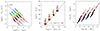 |
Fig. 11. Basic structural planes for Mod-A described by Eqs. (25)–(30). In this particular case the effect of the relative kinetic energy of the incoming object is not included (λ = 0), while the luminosity is simply proportional to the mass via the parameter η and the luminosity effects are neglected (θ = 1). The parameters η and ϵ are randomly varied in the intervals, 0.1 ≤ η ≤ 1.0 and 0.1 ≤ ϵ ≤ 1.0, and finally each parameter is summed up N times. In each panel there are four groups of lines. They correspond to the different infall models with mass MG from which the initial seeds are taken: (from left to right) MG = 106, 108, 1010, 1012 M⊙. Furthermore, in each group there are six dotted lines of different colours according to the age (i.e. redshift) at which the seeds are taken. The colour-coding is as follows: blue (z = 4), green (z = 3), yellow (z = 2), coral (z = 1), magenta (z = 0.5), and black (z = 0). All data for the seeds are listed in Table 2. Left panel: Ie vs Re plane. Middle panel: LV vs σ plane. The dashed line is the best fit limited to the models in four small clouds. Right panel: Re vs Ms plane. The filled circles are the original seed data. |
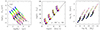 |
Fig. 12. Basic structural planes for Mod-A described by Eqs. (25)–(30). In this case we include the effect of the relative kinetic energy of the incoming object. The parameters η, ϵ, and λ are randomly varied in the intervals 0.1 ≤ η ≤ 0.3, 0.01 ≤ ϵ ≤ 0.03, and 0.1 ≤ λ ≤ 0.3, and summed up N times. In addition to this, the expression for the luminosity contains the parameter θ which is randomly varied at each step in the interval 1 ≤ θ ≤ 3. This parameter is meant to simulate the effect of age of the luminosity of the incoming object. No integration on the number of steps N is performed. The meaning of the symbols and colour-coding are as in Fig. 11. Left panel: Ie vs Re plane. Middle panel: LV vs σ plane. The dashed line is the best fit limited to the models in four small clouds. Right panel: Re vs Ms plane. The filled circles are the original seed data. |
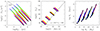 |
Fig. 13. Basic structural planes for Mod-B described by Eqs. (31)–(36). In this particular case we include the effect of the relative kinetic energy of the incoming object. The parameters η, ϵ, and λ are randomly varied in the intervals 0.1 ≤ η ≤ 0.3 and 0.1 ≤ ϵ ≤ 0.3, and are summed up N times. The parameter λ is varied in the range 0 ≤ λ ≤ 0.3 and finally θ = 1 (only the effect of mass is considered). The meaning of the symbols and colour-coding are the same as in Fig. 11. Left panel: Ie vs Re plane. Middle panel: LV vs σ plane. The dashed line is the best fit of the previous Mod-A for comparison. Right panel: Re vs Ms plane. The filled circles are the original seed data. |
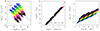 |
Fig. 14. Basic structural planes for Mod-B described by Eqs. (31)–(36) in which the effect of the relative kinetic energy of the incoming object is much stronger than in the case of Fig. 13. The parameters η, ϵ, and λ are randomly varied in the intervals 0.1 ≤ η ≤ 1 and 0.1 ≤ ϵ ≤ 1, and are summed up N times. The parameter λ is varied in the range 0.1 ≤ λ ≤ 2 and finally 1 ≤ θ ≤ 3. The meaning of the symbols and colour-coding are the same as in Fig. 11. Left panel: Ie vs Re plane. Middle panel: LV vs σ plane. The dashed line is the best fit of the previous Mod-A for comparison. Right panel: Re vs Ms plane. The filled circles are the original seed data. |
Inspection of the results presented in this study and many others not shown here for the sake of brevity allow us to say that:
(i) First of all, we emphasize that even if the four cases presented here look alike as far as the general trend of the various relationships, in reality there are important differences that depend on the choice of values assigned to each parameter. Since there are no specific arguments for preferring a particular value with respect to others, we expect a large variety of results to be possible. This is indeed what happens in nature where mergers occur among galaxies of different mass, radius, ages, chemical properties, luminosities, energy budget, evolutionary state, among others. In any case, our choices are made following the general criterion of minimal variations.
(ii) We note that along the lines corresponding to the same galaxy mass MG from which the seeds are derived, the mass Mf increases with N according to the rule Mf(N) = Mi × (1 + Nη). Depending on η (typically ≃0.2) and maximum value N = 1000, we get the maximum mass Mf(1000)≃200Mi. This implies that starting from a initial stage belonging to an object of low mass, say MG ≃ 106 M⊙, successive mergers cannot increase the total mass up to the value typical of high mass galaxies, say a few 1012 M⊙. They hardly go beyond the above limit. One can envisage the following picture: after spontaneous collapse of initial bodies made of baryons and dark mass that are nicely described by the infall models and whose mass may span up to two or three orders of magnitude, at a certain time of their life, mergers with similar bodies of smaller (η < 1) or equal mass (η = 1) may start; the case with η > 1 is similar to the first one in which the roles of the two merging objects are interchanged. For obvious reasons, the case with η ≥ 1 are statistically less frequent. The process goes on so that bigger and bigger galaxies are in place. In this picture the most advantageous cases are mergers of equal mass.
(iii) The variations of luminosity caused by a merger are more difficult to predict. In a galaxy the luminosity is the sum of the partial luminosities emitted by stars of different generations and different chemical composition. Each generation contributes in a way proportional to its mass, age, and chemical composition. The mass of a stellar generation is proportional to the rate of star formation at the time of its birth. In a single stellar generation, the luminosity decreases with the age because of its natural fading as the turnoff mass gets smaller and smaller. For the aims of this study, we can simplify this complicated situation assuming that the mix of stellar populations of different chemical compositions and age can be approximated to a single stellar population of suitable mean chemical composition (indicated here as ⟨SSP⟩), the mass of which equals the total stellar mass of the galaxy. The chemical composition is indicated in the usual notation by means of the mass abundance of Hydrogen (X), Helium (Y) and all other heavy elements lumped together (Z). By definition, X, Y and Z satisfy the condition X + Y + Z = 1. In our case, we can further assume that the mean chemical composition we refer to is close to the solar value, that is [X = 0.700, Y = 0.28, Z = 0.02]. This < SSP> is used to evaluate the time evolution of the luminosity of a galaxy by natural fading caused by the aging of its stellar content. More details on the source of SSPs can be found in D’Onofrio & Chiosi (2024, and references). From the data of Fig. 10 (left panel), we note a fast decline during the first 1.5 to 2 Gyr after the start of star formation, followed by a smooth decline during the rest of the life by a factor of θ = 3 to 5. We adopted θ = 3.
At the time of merger, the two galaxies may have different mass, age, and mean chemical composition, and therefore different luminosities. In the absence of additional star formation at the merger of galaxies A and B, the resulting luminosity will be L = (Ms, ALA + Ms, BLB)/(Ms, A + Ms, B). In analogy, if a new generation of stars is created at the merger with total mass Ms, C and luminosity LC, the resulting new luminosity will be L = (Ms, ALA + Ms, BLB + Ms, CLC)/(Ms, A + Ms, B + Ms, C). In our present models, the bursting star formation at the merger is missing. This is a feature of the model to be improved.
(iv) In the Ie versus Re plane all the groups of models draw lines that are nearly parallel to the ZoE, confirming that they correspond to loci along which virial equilibrium is obtained (imposed). The scatter of the models along each line is due to the scatter of the parameters η, ϵ, λ, and θ when active.
(v) In general, variations of ϵ and λ shift the lines for assigned MG along the direction perpendicular to the ZOE. An increase of these parameter corresponds to a shift from the bottom left corner to the upper right one. It may also happens that a slight variation of the slope of the virial loci towards the ZoE occurs in the region of massive galaxies.
(vi) The L versus σ plane is more intriguing. As expected the gross behaviour is that the luminosity increases with the mass. However, looking at the particular history of a galaxy through its merger sequence, the possibility arises that the luminosity increases while the velocity dispersion decreases. This is the result of the energy exchange among successive mergers. Similar result is found and discussed by Naab et al. (2009). The issue is examined in more detail later on. In any case a large dispersion in this relationship is expected.
(vii) The Re versus Ms relation is expected to increase with the mass both from galaxy to galaxy and also along the merger sequence of each object.
(viii) The results for each case depend on the input parameters η, ϵ, λ, and θ but the general trend is preserved at least for reasonable choices of their values.
(ix) In general, there is not much variation of these relationships with the age of the simulated galaxies and implicitly the redshift at which galaxies are observed.
(x) The theoretical models reasonably correspond to and reproduce the observational data. However, to be used for this purpose, one has to know the relative number of objects of different mass MG and an estimate of the number of mergers that each object of a certain mass can undergo. It is reasonable to assume that in the low mass galaxies only a limited number of mergers can occur, while in the most massive ones a larger number of mergers is plausible. Based on this argument, we suppose that the number of merger increases from 10 for a 106 M⊙ to 1000 for a 1011 M⊙. With aid of this we randomly populate the three planes above by a number of simulated galaxies seen at z = 0 after their last merger episode.
(xi) By construction, models of this type cannot deal with the temporal history of galaxy assembling and star formation because there is no time in the equations governing their structure. This drawback of the models could be cured by estimating the probability that in the course of time mergers can occur among objects of typical masses and sizes confined in certain volume of space. The issue is beyond the aims of this study.
To conclude, the model we are proposing can be considered as a proxy of the merger mechanisms of galaxy formation as far as masses and sizes and other quantities associated to these are concerned. In the following, we compare real galaxies to these mock galaxies to interpret various diagnostic planes such as those examined in this study. To this aim, we compare the results of the analytical model to the same observational samples of galaxies (MaNGA and WINGS at z = 0) as we did for the EAGLE and TNG100 simulations. What we learn from using the analytical merger model and the comparison with the observational data is that even a simple model of galaxy mergers can be useful to investigate the deep physical reasons determining the observed behaviour of real galaxies in the diagnostic planes, projections of the FP, in terms of a unified description.
9. Comparison of our model with the observational data
Fig. 15 shows in the left panel the Ie − Re plane already displayed in Fig. 2 with superposed our mock galaxies of type Mod-B in which a series of mergers from initial seeds of different ages and mass are considered. The parameters of this models are 0.1 ≤ η ≤ 0.3, 0.1 ≤ ϵ ≤ 0.3, 0 ≤ λ ≤ 0.3, and 0.1 ≤ θ = 1.0. This means that in the luminosity only the effect of the increasing mass is considered while that of the age and star formation at the merger are neglected. There is no particular reason for this choice of the parameters. Other similar values would yield similar results. The value of N decreases from the massive to less massive galaxies, to more closely mimic the different merger history of galaxies with different mass. The black dots indicate objects whose seed is taken at the present time while the coloured dots indicate models whose seeds are taken at younger ages (i.e. higher redshift). The colour-coding is as follows: coral (z = 1), yellow (z = 2) and green (z = 3). The observational data are the MaNGA sample (sky-blue dots) and the WINGS sample split according to the age (red for logAge > 9.5 and blue for logAge < 9.5).
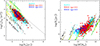 |
Fig. 15. Comparison of simulated galaxies of Mod-B described by Eqs. (31)–(36) with the observational data of MaNGA (see Blanton et al. 2017, and references therein) and WINGS (see text for descriptions). Only E and S0 galaxies are considered here. Left panel: Ie − Re plane where the sky-blue dots are the MaNGA data, while the red and blue filled circles are the WINGS galaxies of different ages, as indicated. The black squares are our simulated mergers starting at z = 0. Similarly, the coloured dots mark mergers at increasing redshift: coral (z = 1), yellow (z = 2), and green (z = 3). The dashed line is the ZoE. Right panel: Re − Ms plane of the same data. In the two panels, the parameters η, ϵ, and λ are randomly varied in the intervals 0.1 ≤ η ≤ 0.3, 0.1 ≤ ϵ ≤ 0.3, and 0 ≤ λ ≤ 0.3. In addition, the expression for the luminosity contains the parameter θ, which is randomly varied at each step in the interval 1 ≤ θ ≤ 3. The value of N changes for the massive and less massive galaxies. The meaning of the symbols and colour-coding are as in Fig. 11. |
The figure indicates that the hierarchical scenario in which galaxies are built up by successive mergers is compatible with the observational data. The Λ-shaped distribution of the galaxies is well reproduced, in particular the long tail formed by the massive galaxies and the clouds of low mass objects. This result can be obtained by limiting the number of possible mergers in galaxies of different mass: a large number of mergers across the whole galaxy age for the more massive objects and fewer mergers for the low mass ones. In this way it is possible to get a very good reproduction of the distribution in the Ie plane. The choice of the number of mergers is based on simple theoretical arguments of statistical nature; we simply say that the more massive galaxies can merge many more galaxies than the less massive objects.
Similarly, the right panel of Fig. 15 indicates that the same simulations can in principle reproduce also the Re − Ms plane. They easily reproduce the tail of the massive galaxies and the cloud-shaped distribution of the smaller ones. The large dispersion of the observational data can be also accounted for.
The same can be said for the relationships shown in the panels of Fig. 16, that is the Ie − σ plane (left panel) and the L − σ plane (right panel). Here, the same limits in the number of mergers has been applied. The values for the parameter η, ϵ, λ and θ are the same as in Fig. 15.
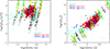 |
Fig. 16. Comparison of simulated galaxies of Mod-B described by Eqs. (31)–(36) with the observational data of MaNGA (see Blanton et al. 2017, and references therein) and WINGS (see text for descriptions). Only E and S0 galaxies are considered. Left panel: Ie − σ plane. Right panel: L − σ plane with the MaNGA and WINGS data, and our artificial galaxy mergers. In the two panels, the colour-coding and the meaning of the symbols are the same as in Fig. 15. The parameters η, ϵ, λ, and θ have the same values as in Fig. 15. |
The L − σ plane (and also the Ms − σ plane not shown here) deserves some comments and explanations. As already mentioned when describing the L − σ plane of Figs. 11, 12 for two Mod-A, and 13 and 14 for the two Mod-B, the luminosity is expected to increase with the velocity dispersion σ as amply confirmed by the observational data, see the classical Faber-Jackson relation, L = L0σα with L0 and α positive. The velocity dispersion is derived from the VT in which the radius Re can be replaced by Re ∝ Ms0.33 (see Tantalo et al. 1998); to a first approximation, it follows that σ2 ∝ Ms0.67. According to a typical mass to luminosity ratio for old galaxies, L ∝ Ms. Therefore L ∝ σ3. The luminosity should only increase with σ. The real slope derived from observational data is about 3.5. The results plotted in Figs. 11, 12, 13 and 14 show that the situation is somewhat more complicated, that is two regimes are possible: at increasing mass the luminosity increases. However, for a system in mechanical equilibrium, that is subjected to the VT, the velocity dispersion may either decrease, if there is not enough energy to disposal, or increase when the amount of the brought-in energy is large enough. In our models, given the mass of the captured object (η), there are two possible sources of energy expressed by the parameters, ϵ (the amount of internal energy brought-in by the captured object) and λ (the amount of kinetic energy brought-in by the captured object). In general, the radius of the composite system is larger or equal to that of the hosting object. If there little energy to disposal (typical of small ϵ and/or λ), in order to reach the equilibrium configuration, part of the energy must be taken from the dispersion velocity which decreases. If ϵ and λ are large enough, the energy required to reach the equilibrium state is taken from the kinetic energy of the infalling object and the velocity dispersion may increase. It goes without saying that all intermediate situations are possible. This effect explains the large dispersion seen in the observational L = L0σα relationship.
Similar results are obtained using our Mod-A simulations, and indeed they produce the same trends. What does change is only the number of mergers required to obtain a given mass.
The comparison of Mod-A and Mod-B with the real observational data shows that our simple model is able to obtain a distribution of galaxies in the FP projections very similar to that obtained with the more sophisticated numerical simulations. The main features of the ScRs are reproduced, such as slopes, scatter and ZoE.
10. Our model in the context of the β − L0′ theory
There is a last step to undertake here. In a series of papers, D’Onofrio et al. (2017); D’Onofrio et al. (2019, 2020), D’Onofrio & Chiosi (2021, 2022, 2023a,b, 2024) proposed a new way of reading the diagnostic planes, projections of the FP of galaxies, in terms of two parameters, β(t) and L′0(t) of the L = L′0(t)σβ(t) relation which was already presented in the introduction and is now repeated here for the sake of completeness:
 (37)
(37)
The parameters L′0(t) and β(t) were found to describe the distribution of galaxies in the various diagnostic planes and to predict the path of a galaxy in any of these planes in the course of evolution, by the natural changes of the various physical quantities defining a galaxy in the FP. We refer to it as the Iβ − L0′ theory. In this section first we refresh the foundations of the β − L0′ theory, derive the β and L′0 for the galaxies of the MaNGA and WINGS samples as well as for our model mergers, and finally compare these results to check whether they are mutually compatible.
In the following we drop the explicit notation of time dependence for the sake of simplicity. The two equations representing the VT and the L = L′0σβ law are
 (38)
(38)
 (39)
(39)
The first equation is the VT itself, where G is the gravitational constant, and kv a term that gives the degree of structural and dynamical non-homology. The presence of kv allows us to write Ms (stellar mass) instead of the total mass MT. kv is a function of the Sérsic index n, that is kv = ((73.32/(10.465 + (n − 0.94)2)) + 0.954) (see Bertin et al. 1992; D’Onofrio et al. 2008, for all details). In the two equations, all other symbols have their usual meaning. In these equations, β and L′0 are time-dependent parameters that depend on the peculiar history of each object.
From these equations one can derive all the mutual relationships existing among the parameters Ms, Re, L, Ie, σ characterizing a galaxy as a function of the β parameter. Although they may be of some interest also in the context of this paper, they are not repeated here. They can be found in D’Onofrio & Chiosi (2024). It suffices to recall that in all these relationships, the slopes depend on β while the proportionality coefficients, in addition to other structural parameters characterizing a galaxy, depend also on L′0. This means that when a galaxy changes its luminosity L, and velocity dispersion σ, and has a given value of β (either positive or negative), the effects of this change in the L − σ plane are propagated in all other projections of the FP. In these planes the galaxies cannot move in whatever directions, but are forced to move only along the directions (slopes) predicted by the β parameter in the above equations. In this sense the β parameter is the link between the FP space and the observed distributions in the FP projections. In addition to this, it is possible to derive an equation holding for each single galaxy that looks like the classical FP. Combining Eq. (39), it is possible to write a FP-like equation involving the parameters β and L′0:
 (40)
(40)
Here ⟨μe⟩ is the mean surface brightness ⟨Ie⟩ expressed in magnitudes, and the coefficients
 (41)
(41)
 (42)
(42)
 (43)
(43)
are written in terms of β and L′0. We note that this is the equation of a plane whose slope depends on β and the zero-point on L′0. The similarity with the FP equation is clear. The novelty is that the FP is an equation derived from the fit of a distribution of real objects, while here each galaxy independently follows an equation formally identical to the classical FP, but of profoundly different physical meaning. In this case, since β and L′0 are time dependent, the equation represents the instantaneous plane on which a generic galaxy is located in the FP space and consequently in all its projections.
Finally, the equation system (39) allows us to determine the values of β and L′0, the two basic evolutionary parameters. Let us write the above equations in the following way:
![Mathematical equation: $$ \begin{aligned} \beta [\log (I_e)+\log (G/k_v)&+\log (M_s/L)+\log (2\pi )+\log (R_e)]\nonumber \\&+ 2\log (L\prime _0) - 2\log (2\pi ) - 4\log (R_e) = 0,\end{aligned} $$](/articles/aa/full_html/2025/02/aa53201-24/aa53201-24-eq51.gif) (44)
(44)
 (45)
(45)
Posing now
 (46)
(46)
 (47)
(47)
 (48)
(48)
 (49)
(49)
we obtain the following system:
 (50)
(50)
 (51)
(51)
with the following solutions:
 (52)
(52)
 (53)
(53)
The key result is that the parameters L, Ms, Re, Ie and σ of a galaxy fully determine its evolution in FP that is encoded in the parameters β and L′0.
Figure 17 (left panel) provides a comparison between the values of β and Ie for the MaNGA and WINGS galaxies and our artificial simulations already presented in Figs. 15 and 16. It is clear that the trend shown by simulations does not fit the more general distribution of β and Ie shown by the observational data, in which β can assume either positive and negative values. The parameter β is very low at very low surface brightness and progressively acquires large values (both negative and positive) for the high surface brightness galaxies. In contrast all the models fall on a single straight line which runs along the border of the distribution of real galaxies in the positive semi-plane. Similar results was found by D’Onofrio & Chiosi (2023a) in the case of infall models.
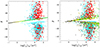 |
Fig. 17. Parameters β for the MaNGA and WINGS data and the models of type Mod-B. Left panel: Ie − β plane for the MaNGA data (sky blue crosses) and WINGS (red dots) and for our merger models of type Mod-B (filled squares of different colours according to the age i.e. redshift) at which the seeds are taken: blue (z = 4), green (z = 3), yellow (z = 2), coral (z = 1), and black (z = 0), i.e. the same colour-coding as in Fig. 11. All the models fall along the same straight line, which coincides with low β-limit of data in the positive semi-plane. Right panel: Same plane after perturbing the theoretical data (see text). The meaning of the symbols and colour-coding are the same as in the left panel. |
Before proceeding further, it is worth commenting on the gap of triangular shape void of galaxies falling in between the distribution on the positive and negative semi-planes. It is easy to check that this gap corresponds in the Ie − Re plane to objects of relatively low surface brightness Ie (and also luminosities) and intermediate radii Re that do not exist in our observational sample. They should correspond to the so-called diffuse galaxies that are difficult to identify (and perhaps are rare in the sky). So the gap is not a problem here and is left aside.
To understand the causes of the above disagreement a few remarks may be helpful. The correct comparison should take into account the following facts: (i) the luminosity of galaxies of our models does not consider the variations of the M/L ratios present among real galaxies. The luminosity of a galaxy primarily depends on its mass, but it also depends on other factors, such as star forming episodes, star formation quenching, natural fading). Taking all of them in account correctly is a cumbersome affair; (ii) the errors on the observed structural parameters that can be as high as 20%; (iii) the radii evaluated by our simulations that do not strictly correspond to the real effective radii measured in the data. In order to somehow include such effects in our simulations of mergers, we decided to apply a random variation in the Re and Ie parameters of the model galaxies. The maximum variation of Re is ≃0.4 (in log units), and the maximum variation of Ie is ≃1 (in log units). These variations on Re and Ie soon propagate to β and L′0. The results are shown in the right panel of Fig. 17 limited to β. Now the theoretical values of β spread out over the whole Ie − β plane in that closely mimicking the observational data. Therefore at least part of the scatter in the β − Ie can be attributed to uncertainties in the determination of Ie and Re.
Another point to consider is related to the definition of L′0 and β. Relations (53) show that β depends on log L′0 which in turn contains the quantity 1 − 2A′/A at the denominator, where A′ is 2log σ while the A, expressed by means of Ie, G/kv, Ms, L and Re, can also be reduced to 2log σ. Therefore, β should diverge when the denominator tends to zero. So high values of β and L′0 should be the signature that the two derivation of σ are in mutual agreement and implicitly that the system is mechanical equilibrium. Unfortunately, Ie, Ms, and Re, are all derived from the luminosity and its profile in the central region so that their are likely affected by some uncertainty. The quantity kv is an indirect evaluation of the morphology of the galaxy, which is unknown in most cases, at least in the samples under examination, so that kv is also highly uncertain. Catching the right combination of all these parameters is highly unlikely. To cast light on this issue we looked at the relative number of galaxies as a function of β. In our observational sample (only MaNGA to avoid contamination by other sources), we count 414 ETGs (only E galaxies, S0 are left aside) and 2075 LTGs (Sa+Sb+Sc lumped together). These are the same galaxies already shown in Fig. 17. Their number distribution as a function of β is shown in Fig. 18. The histograms displays the two populations with different colours (red for ETGs and blue for LTGs) in steps of 10 for β. The ETGs population is centered at small values of beta (−20 ≤ β − 10), while LTGs peak in between −20 ≤ β ≤ 10). In brief ETGs are more shifted to the negative domain while LTGs are more shifted towards the positive domain. Finally both ETGs and LTGs have tails towards high values of |β| on both semi-planes. Assuming as tail all galaxies falling below β = −40 and above β = 40, the estimated total fractions in the tails and peaks amount to 0.15 (left), 0.45 (peak), 0.27 (right) for ETGs and 0.09 (left), 0.43 (peak) and 0.09 (right) for LTGs. Apparently the great majority of galaxies have parameters that cannot be used to infer their dynamical conditions. However, the typical dynamical timescale for a galaxy is about 0.5 Gyr. This is also the timescale required to lose memory of any dynamical perturbation similar to a merger. On the other hand, if the merger induces star formation accompanied by a variation in total luminosity, about 3 Gyr is the timescale required to lose memory of the luminosity perturbation (see the data in Fig. 10). It follows that while the memory of the dynamical event is quickly lost, that of the luminosity variations lasts longer. Therefore, all quantities that directly or indirectly derive from the luminosity keep memory of the event for longer time and therefore the dynamical conditions of the system cannot be safely ascertained by this kind of arguments.
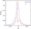 |
Fig. 18. Histogram of the percentage distribution of β of the MaNGA galaxies. The red line shows the ETGs (only E galaxies, NT = 414), the blue line the LTGs (Sa+Sb+Sc, NT = 2075). |
To conclude, mergers alone cannot explain the whole story encrypted in the ScRs. Luminosity effects should also be taken into consideration in a much better way than what has been done so far in order to explain the scatter present in the β − Ie plane (observational data and theoretical models). Work is in progress along this line.
11. Conclusions
Three are the aims of this study: (i) to analyse in detail the observational sample of MaNGA galaxies and to compare it with two theoretical databases of galaxy models in the ΛCDM hierarchical scenario of structure formation EAGLE and Illustris-TNG100; (ii) to propose and validate a simple analytical model of galaxy formation in the hierarchical scheme aimed to be a proxy of real galaxies and at the same time of the galaxy models obtained by the large-scale cosmo-hydro-dynamical simulations; (iii) to analyse the various projection planes of the galaxies’ FPs in the light of the theoretical results at our disposal (large-scale simulations and the simple analytical model) in a unitary conceptual framework. In the following we briefly comment on the three topics.
(i) There is a satisfactory agreement between the MaNGA data and the results of the large-scale theoretical simulations EAGLE and Illustris-TNG100. There are some differences, but they do not invalidate the general agreement. More precisely, the radii Re predicted by EAGLE are a bit greater than those of MaNGA, while those of Illustris-TNG100 are a bit smaller. There is the important result that the radii Re increase at decreasing redshift; in other words, galaxy size increases as they become older. The same is true for the galaxy mass, which is found to increase as the redshift decreases. The relation Re − Ms varies with time. At high redshift the relationship seems to disappear. Objects with mass in excess of 1010 M⊙ are rare; the bulk of galaxies have lower masses and their radii span a large range of values with a mean value either nearly constant or weakly increasing with mass. It is only at redshift z ≤ 2 − 1.5, when massive galaxies are numerous, that the standard Re − Ms relations fall in place with a positive slope and small scatter around it. Finally, the rate of star formation either decreases or is nearly zero as the redshift tends to zero. This is particularly true for ETGs, while the rate remains active at moderate levels of activity in the late-type objects. Dwarf galaxies belong to a separate group that is not included in our analysis.
(ii) In order to better clarify the role played by mergers in shaping the above trends and results without being forced to perform intensive numerical computing with the standard N-Body hydro-dynamical codes, we proposed a simple model of mergers. To avoid misunderstanding, it is better to clarify that our model mergers are not intended to compete with those from detailed large-scale numerical simulations. They must be considered as a simple tool to get quick understanding of the physical causes of why galaxies populate the diagnostic planes, projections of the FP, in the way they do. The model stands on the VT, a physical condition at which galaxies are during most of their life, makes use of parameters to quantify the mass of the captured object, the energy injection, and the energy sharing, the effect on the radius, velocity dispersion, luminosity, and specific intensity. The formalism in use is simple and allows us to get results at no cost in terms of computing time and resources. A large number of simulations are made at varying parameters, and with the aid of these simulations the usual diagnostic planes are derived. The results are found to be fully compatible with both observational data and extensive N-Body hydro-dynamical simulations. We limit ourselves here to highlighting that the model provides a simple explanation for the larger dispersion shown by the data in the diagnostic planes (for instance the Re − Ms and L − σ planes). They also cast light on some unexpected sub-trends found in the L − Ms, L − σ, and Ms − σ planes, and they can explain the Λ-like distribution in the Ie − Re plane. Above all, they better clarify the role of mergers in shaping all the relations found in the diagnostic planes. At present, the model cannot deal with or predict the behaviour of star formation. Work is in progress to cope with this. Despite its simplicity, the model of mergers we are proposing can complement or even guide more complex simulations.
To conclude, we can say that the method and results presented in this study can be taken as the starting point of more sophisticated analyses, in which the histories of star formation and luminosity in turn are explicitly taken into account. Thanks to its simplicity, our approach offers some advantages with respect to numerical simulations. However, it cannot yield the precise predictions of these latter. Even so, it can predict the effects of different physical phenomena on the observed ScRs.
Acknowledgments
M.D. and F.T. thank the Department of Physics and Astronomy of the Padua University for the financial support. C.C. thanks the Padua University for the hospitality.
References
- Adams, F. C. 2019, Phys. Rep., 807, 1 [NASA ADS] [CrossRef] [Google Scholar]
- Agertz, O., & Kravtsov, A. V. 2015, ApJ, 804, 18 [NASA ADS] [CrossRef] [Google Scholar]
- Bender, R., Burstein, D., & Faber, S. M. 1992, ApJ, 399, 462 [NASA ADS] [CrossRef] [Google Scholar]
- Bernardi, M., Sheth, R. K., Annis, J., et al. 2003, ApJ, 125, 1866 [CrossRef] [Google Scholar]
- Bernardi, M., Roche, N., Shankar, F., & Sheth, R. K. 2011, MNRAS, 412, L6 [NASA ADS] [CrossRef] [Google Scholar]
- Bertin, G., Saglia, R. P., & Stiavelli, M. 1992, ApJ, 384, 423 [NASA ADS] [CrossRef] [Google Scholar]
- Biviano, A., Moretti, A., Paccagnella, A., et al. 2017, A&A, 607, A81 [NASA ADS] [CrossRef] [EDP Sciences] [Google Scholar]
- Blanton, M. R., Bershady, M. A., Abolfathi, B., et al. 2017, AJ, 154, 28 [Google Scholar]
- Boylan-Kolchin, M., Ma, C.-P., & Quataert, E. 2006, MNRAS, 369, 1081 [CrossRef] [Google Scholar]
- Bundy, K., Bershady, M. A., Law, D. R., et al. 2015, ApJ, 798, 7 [Google Scholar]
- Burstein, D., Bender, R., Faber, S. M., & Nolthenius, R. 1995, Astrophys. Lett. Commun., 31, 95 [NASA ADS] [Google Scholar]
- Cannarozzo, C., Leauthaud, A., Oyarzún, G. A., et al. 2023, MNRAS, 520, 5651 [NASA ADS] [CrossRef] [Google Scholar]
- Cariddi, S., D’Onofrio, M., Fasano, G., et al. 2018, A&A, 609, A133 [NASA ADS] [CrossRef] [EDP Sciences] [Google Scholar]
- Cava, A., Bettoni, D., Poggianti, B. M., et al. 2009, A&A, 495, 707 [NASA ADS] [CrossRef] [EDP Sciences] [Google Scholar]
- Chiosi, C., & Carraro, G. 2002, MNRAS, 335, 335 [NASA ADS] [CrossRef] [Google Scholar]
- Chiosi, C., D’Onofrio, M., & Piovan, L. 2023, A&A, 678, A12 [NASA ADS] [CrossRef] [EDP Sciences] [Google Scholar]
- Courteau, S., Dutton, A. A., van den Bosch, F. C., et al. 2007, ApJ, 671, 203 [Google Scholar]
- Damjanov, I., McCarthy, P. J., Abraham, R. G., et al. 2009, ApJ, 695, 101 [Google Scholar]
- Desroches, L.-B., Quataert, E., Ma, C.-P., & West, A. A. 2007, MNRAS, 377, 402 [NASA ADS] [CrossRef] [Google Scholar]
- D’Onofrio, M., & Chiosi, C. 2021, Universe, 8, 8 [CrossRef] [Google Scholar]
- D’Onofrio, M., & Chiosi, C. 2022, A&A, 661, A150 [NASA ADS] [CrossRef] [EDP Sciences] [Google Scholar]
- D’Onofrio, M., & Chiosi, C. 2023a, A&A, 674, A156 [NASA ADS] [CrossRef] [EDP Sciences] [Google Scholar]
- D’Onofrio, M., & Chiosi, C. 2023b, A&A, 675, A186 [NASA ADS] [CrossRef] [EDP Sciences] [Google Scholar]
- D’Onofrio, M., & Chiosi, C. 2024, A&A, 687, A126 [NASA ADS] [CrossRef] [EDP Sciences] [Google Scholar]
- D’Onofrio, M., Valentinuzzi, T., Secco, L., Caimmi, R., & Bindoni, D. 2006, New Astron. Rev., 50, 447 [CrossRef] [Google Scholar]
- D’Onofrio, M., Fasano, G., Varela, J., et al. 2008, ApJ, 685, 875 [CrossRef] [Google Scholar]
- D’Onofrio, M., Bindoni, D., Fasano, G., et al. 2014, A&A, 572, A87 [NASA ADS] [CrossRef] [EDP Sciences] [Google Scholar]
- D’Onofrio, M., Cariddi, S., Chiosi, C., Chiosi, E., & Marziani, P. 2017, ApJ, 838, 163 [CrossRef] [Google Scholar]
- D’Onofrio, M., Sciarratta, M., Cariddi, S., Marziani, P., & Chiosi, C. 2019, ApJ, 875, 103 [Google Scholar]
- D’Onofrio, M., Chiosi, C., Sciarratta, M., & Marziani, P. 2020, A&A, 641, A94 [NASA ADS] [CrossRef] [EDP Sciences] [Google Scholar]
- D’Onofrio, M., Marziani, P., Chiosi, C., & Negrete, C. A. 2024, Universe, 10, 254 [CrossRef] [Google Scholar]
- Drory, N., MacDonald, N., Bershady, M. A., et al. 2015, AJ, 149, 77 [CrossRef] [Google Scholar]
- Faber, S. M., & Jackson, R. E. 1976, ApJ, 204, 668 [Google Scholar]
- Fan, L., Lapi, A., Bressan, A., et al. 2010, ApJ, 718, 1460 [NASA ADS] [CrossRef] [Google Scholar]
- Fasano, G., Marmo, C., Varela, J., et al. 2006, A&A, 445, 805 [NASA ADS] [CrossRef] [EDP Sciences] [Google Scholar]
- Fasano, G., Vanzella, E., Dressler, A., et al. 2012, MNRAS, 420, 926 [Google Scholar]
- Ferrero, I., Navarro, J. F., Abadi, M. G., et al. 2017, MNRAS, 464, 4736 [Google Scholar]
- Fritz, J., Poggianti, B. M., Bettoni, D., et al. 2007, A&A, 470, 137 [NASA ADS] [CrossRef] [EDP Sciences] [Google Scholar]
- Furlong, M., Bower, R. G., Crain, R. A., et al. 2017, MNRAS, 465, 722 [Google Scholar]
- Genel, S., Nelson, D., Pillepich, A., et al. 2018, MNRAS, 474, 3976 [Google Scholar]
- Gullieuszik, M., Poggianti, B., Fasano, G., et al. 2015, A&A, 581, A41 [NASA ADS] [CrossRef] [EDP Sciences] [Google Scholar]
- Huertas-Company, M., Rodriguez-Gomez, V., Nelson, D., et al. 2019, MNRAS, 489, 1859 [NASA ADS] [CrossRef] [Google Scholar]
- Hyde, J. B., & Bernardi, M. 2009, MNRAS, 396, 1171 [NASA ADS] [CrossRef] [Google Scholar]
- Krajnović, D., Emsellem, E., den Brok, M., et al. 2018, MNRAS, 477, 5327 [Google Scholar]
- Lange, R., Moffett, A. J., Driver, S. P., et al. 2016, MNRAS, 462, 1470 [NASA ADS] [CrossRef] [Google Scholar]
- McAlpine, S., Helly, J. C., Schaller, M., et al. 2016, Astron. Comput., 15, 72 [NASA ADS] [CrossRef] [Google Scholar]
- Montero-Dorta, A. D., Shu, Y., Bolton, A. S., Brownstein, J. R., & Weiner, B. J. 2016, MNRAS, 456, 3265 [NASA ADS] [CrossRef] [Google Scholar]
- Moretti, A., Poggianti, B. M., Fasano, G., et al. 2014, A&A, 564, A138 [NASA ADS] [CrossRef] [EDP Sciences] [Google Scholar]
- Moretti, A., Gullieuszik, M., Poggianti, B., et al. 2017, A&A, 599, A81 [NASA ADS] [CrossRef] [EDP Sciences] [Google Scholar]
- Naab, T., Johansson, P. H., & Ostriker, J. P. 2009, ApJ, 699, L178 [Google Scholar]
- Nelson, D., Pillepich, A., Springel, V., et al. 2018, MNRAS, 475, 624 [Google Scholar]
- Nigoche-Netro, A., Aguerri, J. A. L., Lagos, P., et al. 2011, A&A, 534, A61 [NASA ADS] [CrossRef] [EDP Sciences] [Google Scholar]
- Oegerle, W. R., & Hoessel, J. G. 1991, ApJ, 375, 15 [NASA ADS] [CrossRef] [Google Scholar]
- Pignatelli, E., Fasano, G., & Cassata, P. 2006, A&A, 446, 373 [NASA ADS] [CrossRef] [EDP Sciences] [Google Scholar]
- Pillepich, A., Springel, V., Nelson, D., et al. 2018a, MNRAS, 473, 4077 [Google Scholar]
- Pillepich, A., Nelson, D., Hernquist, L., et al. 2018b, MNRAS, 475, 648 [Google Scholar]
- Quenneville, M. E., Blakeslee, J. P., Ma, C.-P., et al. 2024, MNRAS, 527, 249 [Google Scholar]
- Rodriguez-Gomez, V., Snyder, G. F., Lotz, J. M., et al. 2019, MNRAS, 483, 4140 [NASA ADS] [CrossRef] [Google Scholar]
- Samir, R. M., Takey, A., & Shaker, A. A. 2020, Ap&SS, 365, 142 [NASA ADS] [CrossRef] [Google Scholar]
- Sánchez Almeida, J. 2020, MNRAS, 495, 78 [Google Scholar]
- Sanders, R. H. 2010, MNRAS, 407, 1128 [CrossRef] [Google Scholar]
- Schaye, J., Crain, R. A., Bower, R. G., et al. 2015, MNRAS, 446, 521 [Google Scholar]
- Secco, L. 2001, New Astron., 6, 339 [NASA ADS] [CrossRef] [Google Scholar]
- Shankar, F., Marulli, F., Bernardi, M., et al. 2013, MNRAS, 428, 109 [NASA ADS] [CrossRef] [Google Scholar]
- Shen, S., Mo, H. J., White, S. D. M., et al. 2003, MNRAS, 343, 978 [NASA ADS] [CrossRef] [Google Scholar]
- Smee, S. A., Gunn, J. E., Uomoto, A., et al. 2013, AJ, 146, 32 [Google Scholar]
- Springel, V., Pakmor, R., Pillepich, A., et al. 2018, MNRAS, 475, 676 [Google Scholar]
- Tantalo, R. 2005, Astrophys. Space Sci. Lib., 327, 235 [NASA ADS] [CrossRef] [Google Scholar]
- Tantalo, R., Chiosi, C., Bressan, A., Marigo, P., & Portinari, L. 1998, A&A, 335, 823 [NASA ADS] [Google Scholar]
- Valentinuzzi, T., Woods, D., Fasano, G., et al. 2009, A&A, 501, 851 [NASA ADS] [CrossRef] [EDP Sciences] [Google Scholar]
- van der Wel, A., Bezanson, R., D’Eugenio, F., et al. 2021, ApJS, 256, 44 [NASA ADS] [CrossRef] [Google Scholar]
- Varela, J., D’Onofrio, M., Marmo, C., et al. 2009, A&A, 497, 667 [NASA ADS] [CrossRef] [EDP Sciences] [Google Scholar]
- Vogelsberger, M., Genel, S., Springel, V., et al. 2014a, Nature, 509, 177 [Google Scholar]
- Vogelsberger, M., Genel, S., Springel, V., et al. 2014b, MNRAS, 444, 1518 [Google Scholar]
All Tables
All Figures
|
Fig. 1. Comparison of the Ie − Re plane for the WINGS and MaNGA data. The black symbols mark the whole WINGS dataset, while the green symbols indicate the MaNGA data. All morphological types are included for both datasets. |
| In the text | |
|
Fig. 2. Comparison of the Ie − Re plane with the MaNGA data and simulations: EAGLE in the left panel and TNG100 in the right panel. The green crosses mark the MaNGA data for all morphological types, while the red circles are for the EAGLE data and the blue circles are for TNG100. |
| In the text | |
|
Fig. 3. Comparison of the Re − Ms plane with the MaNGA data and simulations. In the left panel the EAGLE models, in the right panel the TNG100 models. The colour-coding and symbols are as before. |
| In the text | |
|
Fig. 4. Comparison of the L − σ plane with MaNGA data and simulations. In the left panel the EAGLE models, in the right panel the TNG100 models. The colour-coding and symbols are as before. |
| In the text | |
|
Fig. 5. Comparison of the Ie − Re, L − σ, and Re − Ms planes for the LEGA-C data (green dots) and the TNG100 simulations (blue dots). The data and models refer to galaxies observed and/or predicted at redshift z = 1. |
| In the text | |
|
Fig. 6. Comparison between EAGLE (red dots) and TNG (blue dots) at z = 1 (the group of four panels at the left) and z = 2 (the group of four panels at the right) in four ScRs: the Ie − Re plane (top left), the Ie − σ plane (top right), the Re − Ms plane (bottom left), and the SFR–Ms plane (bottom right). |
| In the text | |
|
Fig. 7. Comparison between EAGLE and TNG at z = 3 (left panel) and z = 4 (right panel). The symbols and diagrams are as in Fig. 6. |
| In the text | |
|
Fig. 8. Mean evolutionary path of galaxies in the EAGLE simulations. The blue dots and lines give the mean path of the galaxies with current masses higher than 1011 M⊙, while the red dots and lines those for the masses lower than 109 M⊙. The variables Re, Ms, Ie, and β are plotted against the redshift z. |
| In the text | |
|
Fig. 9. Mean evolutionary path of galaxies in the TNG simulations. The colours, symbols, and diagrams are as in Fig. 8. |
| In the text | |
|
Fig. 10. Mass-to-luminosity and luminosity-to-mass ratios as functions of the age (left panel) and the luminosity-to-mass ratio as a function of the stellar mass Ms (right panel). The masses and luminosities are in solar units, the age is in Gyr. Left panel: In the panel the solid red and blue lines are the Ms/LV and Lv/Ms ratios, respectively, for an infall model of asymptotic mass of 1010 M⊙ calculated by the authors (see Chiosi et al. 2023, and references), while the black dots along each line are the same, but for a SSP with solar chemical composition taken from the Padova library (Tantalo 2005). The straight lines are the best fit of the relations. Right panel: Ms/LV ratio for two infall models with different masses. For each case the stellar mass increases along each curve from left to right. The two straight lines are the best fit of the data (see text for more details). |
| In the text | |
|
Fig. 11. Basic structural planes for Mod-A described by Eqs. (25)–(30). In this particular case the effect of the relative kinetic energy of the incoming object is not included (λ = 0), while the luminosity is simply proportional to the mass via the parameter η and the luminosity effects are neglected (θ = 1). The parameters η and ϵ are randomly varied in the intervals, 0.1 ≤ η ≤ 1.0 and 0.1 ≤ ϵ ≤ 1.0, and finally each parameter is summed up N times. In each panel there are four groups of lines. They correspond to the different infall models with mass MG from which the initial seeds are taken: (from left to right) MG = 106, 108, 1010, 1012 M⊙. Furthermore, in each group there are six dotted lines of different colours according to the age (i.e. redshift) at which the seeds are taken. The colour-coding is as follows: blue (z = 4), green (z = 3), yellow (z = 2), coral (z = 1), magenta (z = 0.5), and black (z = 0). All data for the seeds are listed in Table 2. Left panel: Ie vs Re plane. Middle panel: LV vs σ plane. The dashed line is the best fit limited to the models in four small clouds. Right panel: Re vs Ms plane. The filled circles are the original seed data. |
| In the text | |
|
Fig. 12. Basic structural planes for Mod-A described by Eqs. (25)–(30). In this case we include the effect of the relative kinetic energy of the incoming object. The parameters η, ϵ, and λ are randomly varied in the intervals 0.1 ≤ η ≤ 0.3, 0.01 ≤ ϵ ≤ 0.03, and 0.1 ≤ λ ≤ 0.3, and summed up N times. In addition to this, the expression for the luminosity contains the parameter θ which is randomly varied at each step in the interval 1 ≤ θ ≤ 3. This parameter is meant to simulate the effect of age of the luminosity of the incoming object. No integration on the number of steps N is performed. The meaning of the symbols and colour-coding are as in Fig. 11. Left panel: Ie vs Re plane. Middle panel: LV vs σ plane. The dashed line is the best fit limited to the models in four small clouds. Right panel: Re vs Ms plane. The filled circles are the original seed data. |
| In the text | |
|
Fig. 13. Basic structural planes for Mod-B described by Eqs. (31)–(36). In this particular case we include the effect of the relative kinetic energy of the incoming object. The parameters η, ϵ, and λ are randomly varied in the intervals 0.1 ≤ η ≤ 0.3 and 0.1 ≤ ϵ ≤ 0.3, and are summed up N times. The parameter λ is varied in the range 0 ≤ λ ≤ 0.3 and finally θ = 1 (only the effect of mass is considered). The meaning of the symbols and colour-coding are the same as in Fig. 11. Left panel: Ie vs Re plane. Middle panel: LV vs σ plane. The dashed line is the best fit of the previous Mod-A for comparison. Right panel: Re vs Ms plane. The filled circles are the original seed data. |
| In the text | |
|
Fig. 14. Basic structural planes for Mod-B described by Eqs. (31)–(36) in which the effect of the relative kinetic energy of the incoming object is much stronger than in the case of Fig. 13. The parameters η, ϵ, and λ are randomly varied in the intervals 0.1 ≤ η ≤ 1 and 0.1 ≤ ϵ ≤ 1, and are summed up N times. The parameter λ is varied in the range 0.1 ≤ λ ≤ 2 and finally 1 ≤ θ ≤ 3. The meaning of the symbols and colour-coding are the same as in Fig. 11. Left panel: Ie vs Re plane. Middle panel: LV vs σ plane. The dashed line is the best fit of the previous Mod-A for comparison. Right panel: Re vs Ms plane. The filled circles are the original seed data. |
| In the text | |
|
Fig. 15. Comparison of simulated galaxies of Mod-B described by Eqs. (31)–(36) with the observational data of MaNGA (see Blanton et al. 2017, and references therein) and WINGS (see text for descriptions). Only E and S0 galaxies are considered here. Left panel: Ie − Re plane where the sky-blue dots are the MaNGA data, while the red and blue filled circles are the WINGS galaxies of different ages, as indicated. The black squares are our simulated mergers starting at z = 0. Similarly, the coloured dots mark mergers at increasing redshift: coral (z = 1), yellow (z = 2), and green (z = 3). The dashed line is the ZoE. Right panel: Re − Ms plane of the same data. In the two panels, the parameters η, ϵ, and λ are randomly varied in the intervals 0.1 ≤ η ≤ 0.3, 0.1 ≤ ϵ ≤ 0.3, and 0 ≤ λ ≤ 0.3. In addition, the expression for the luminosity contains the parameter θ, which is randomly varied at each step in the interval 1 ≤ θ ≤ 3. The value of N changes for the massive and less massive galaxies. The meaning of the symbols and colour-coding are as in Fig. 11. |
| In the text | |
|
Fig. 16. Comparison of simulated galaxies of Mod-B described by Eqs. (31)–(36) with the observational data of MaNGA (see Blanton et al. 2017, and references therein) and WINGS (see text for descriptions). Only E and S0 galaxies are considered. Left panel: Ie − σ plane. Right panel: L − σ plane with the MaNGA and WINGS data, and our artificial galaxy mergers. In the two panels, the colour-coding and the meaning of the symbols are the same as in Fig. 15. The parameters η, ϵ, λ, and θ have the same values as in Fig. 15. |
| In the text | |
|
Fig. 17. Parameters β for the MaNGA and WINGS data and the models of type Mod-B. Left panel: Ie − β plane for the MaNGA data (sky blue crosses) and WINGS (red dots) and for our merger models of type Mod-B (filled squares of different colours according to the age i.e. redshift) at which the seeds are taken: blue (z = 4), green (z = 3), yellow (z = 2), coral (z = 1), and black (z = 0), i.e. the same colour-coding as in Fig. 11. All the models fall along the same straight line, which coincides with low β-limit of data in the positive semi-plane. Right panel: Same plane after perturbing the theoretical data (see text). The meaning of the symbols and colour-coding are the same as in the left panel. |
| In the text | |
|
Fig. 18. Histogram of the percentage distribution of β of the MaNGA galaxies. The red line shows the ETGs (only E galaxies, NT = 414), the blue line the LTGs (Sa+Sb+Sc, NT = 2075). |
| In the text | |
Current usage metrics show cumulative count of Article Views (full-text article views including HTML views, PDF and ePub downloads, according to the available data) and Abstracts Views on Vision4Press platform.
Data correspond to usage on the plateform after 2015. The current usage metrics is available 48-96 hours after online publication and is updated daily on week days.
Initial download of the metrics may take a while.