| Issue |
A&A
Volume 675, July 2023
|
|
|---|---|---|
| Article Number | A186 | |
| Number of page(s) | 21 | |
| Section | Extragalactic astronomy | |
| DOI | https://doi.org/10.1051/0004-6361/202345940 | |
| Published online | 19 July 2023 | |
The scaling relations of galaxies back in time: The road toward virialization
Department of Physics and Astronomy, University of Padua, Vicolo Osservatorio 3, 35122 Padova, Italy
e-mail: This email address is being protected from spambots. You need JavaScript enabled to view it.
; This email address is being protected from spambots. You need JavaScript enabled to view it.
Received:
19
January
2023
Accepted:
6
June
2023
Abstract
Context. The structural scaling relations (SSRs) of galaxies, that is, the observed correlations between effective radius, effective surface intensity, and velocity dispersion, are important tools for understanding how evolution proceeds.
Aims. In this paper, we aim to demonstrate that the evolution of the SSRs back in time is governed by a combination of virial theorem (VT) and the relation L = L0′(t)σβ(t), where the parameters β and L0′ vary with time and from galaxy to galaxy.
Methods. Using the WINGS database for the galaxies at redshift z = 0 and the Illustris-1 and IllustrisTNG databases of artificial galaxies, for the galaxies up to redshift z = 4, we analyse the SSRs back in time and, by means of simple algebraic expressions for L0′ and β (functions of time and other physical quantities), we derive the expected paths followed by galaxies in the various SSRs toward the distributions observed at z = 0.
Results. The distribution of galaxies in the SSRs is ultimately related to the evolution in luminosity and velocity dispersion, which are empirically mirrored by the L = L0′(t)σβ(t) law. Furthermore, the β parameter works as a thermometer of the virialization of a galaxy. This parameter can assume either positive or negative values, and its absolute value attains high values when the galaxy is close to the virial condition, while it tends to zero when the galaxy is far from this condition.
Conclusions. As the SSRs change with time, the method proposed in this paper allows us to decipher the temporal evolution of galaxies.
Key words: galaxies: evolution / galaxies: fundamental parameters / galaxies: general
© The Authors 2023
 Open Access article, published by EDP Sciences, under the terms of the Creative Commons Attribution License (https://creativecommons.org/licenses/by/4.0), which permits unrestricted use, distribution, and reproduction in any medium, provided the original work is properly cited.
This article is published in open access under the Subscribe to Open model. This email address is being protected from spambots. You need JavaScript enabled to view it. to support open access publication.
1. Introduction
The structural scaling relations (SSRs) of galaxies, that is, the mutual correlations between the main measured structural parameters, such as the effective radius Re, the effective surface intensity Ie, the total stellar mass Ms, the luminosity L, and the central velocity dispersion σ, were recognized long ago as important tools for understanding the evolution of these stellar systems and for deriving fundamental cosmological information (see e.g., Faber & Jackson 1976; Kormendy 1977; Dressler et al. 1987; Djorgovski & Davis 1987). In particular, the SSRs of early-type galaxies (ETGs), the obtention of which is relatively straightforward, have been used in the past as distance indicators for measuring the Hubble constant (see e.g., Dressler 1987), for testing the expansion of the Universe (see e.g., Pahre et al. 1996), for mapping the velocity fields of galaxies (see e.g., Dressler & Faber 1990; Courteau et al. 1993), and for measuring the variation of the mass-to-light ratio across time (see e.g., Prugniel & Simien 1996; van Dokkum & Franx 1996; Busarello et al. 1998; Franx et al. 2008).
Among the various SSRs, the fundamental plane (FP) relation for the ETGs (Djorgovski & Davis 1987; Dressler et al. 1987), log Re = a log σ + b log Ie + c, is probably the most studied of the last 30 years. The tilt of this relation with respect to the prediction of virial theorem (VT) has been the subject of many studies (see e.g., Faber et al. 1987; Ciotti 1991; Jorgensen et al. 1996; Cappellari et al. 2006; D’Onofrio et al. 2006; Bolton et al. 2007), invoking different physical mechanisms at work; to mention but a few: (i) the systematic change of the stellar mass-to-light ratio (Ms/L) (see e.g., Faber et al. 1987; van Dokkum & Franx 1996; Cappellari et al. 2006; van Dokkum & van der Marel 2007; Holden et al. 2010; de Graaff et al. 2021); (ii) the structural and dynamical non-homology of ETGs (see e.g., Prugniel & Simien 1997; Busarello et al. 1998; Trujillo et al. 2004; D’Onofrio et al. 2008); (iii) the dark matter content and distribution (see e.g., Ciotti et al. 1996; Borriello et al. 2003; Tortora et al. 2009; Taranu et al. 2015; de Graaff et al. 2021); (iv) the star formation history (SFH) and initial mass function (IMF) (see e.g., Renzini & Ciotti 1993; Chiosi et al. 1998; Chiosi & Carraro 2002; Allanson et al. 2009); (v) the effects of environment (see e.g., Lucey et al. 1991; de Carvalho & Djorgovski 1992; Bernardi et al. 2003; D’Onofrio et al. 2008; La Barbera et al. 2010; Ibarra-Medel & López-Cruz 2011; Samir et al. 2016); (vi) the effects of dissipationless mergers (Nipoti et al. 2003); (vii) the gas dissipation (Robertson et al. 2006; viii) the irregular sequence of mergers with progressively decreasing mass ratios (Novak 2008); and (ix) the multiple dry mergers of spiral galaxies (Taranu et al. 2015).
A similar long list can be compiled for the small intrinsic scatter of the FP (≈0.05 dex in the V-band), where among the claimed possible physical causes, we have: (1) the variation in the formation epoch; (2) the dark matter content; (3) the metallicity or age trends; (4) the variations of the mass-to-light ratio M/L (see e.g., Faber et al. 1987; Gregg 1992; Guzman et al. 1993; Forbes et al. 1998; Bernardi et al. 2003; Reda et al. 2005; Cappellari et al. 2006; Bolton et al. 2008; Auger et al. 2010; Magoulas et al. 2012), and so on.
Despite all these efforts, it is still unclear today as to why the FP is so tight and uniform when seen edge-on, while in its projections (i.e., in the Ie–Re, the Ie–σ, and Re–σ planes) the distribution of galaxies presents well-defined structures, where regions with large clumps of objects and big scatter are observed together with regions where no galaxies are present, the so-called zone of exclusions (ZOE), and where clear nonlinear distributions are well visible. The mutual dependence of the SSRs, the peculiar shape of the observed distributions, and the link among the various FP projections have never found a single and robust explanation in which the tilt and the scatter of the FP are understood.
The same difficulties are encountered when we consider one particular projection of the FP: the Faber-Jackson (FJ) relation (Faber & Jackson 1976), which is, the correlation observed between the total luminosity L and the central velocity dispersion σ. Even in this case, the observed trend is not that predicted by the VT. In addition to this, it has been shown that the L − σ relation is not consistent with the distribution observed in the Ie − Re plane, in the sense that it is not possible to transform one space into the other (and vice versa) while adopting the observed classical correlations (see e.g., D’Onofrio & Chiosi 2021).
In other words, there are many underlying questions behind the nature of the SSRs of galaxies. We do not have a single explanation for the tilt of the FP and the shapes of the distributions observed in its projections. We are not able to reconcile the FJ relation and the Ie − Re plane. We cannot account for the mutual relationship among the various projections of the FP and we do not understand how these planes are mutually linked each other. We do not know wow the SSRs change going back in time and why the FP is so tight.
D’Onofrio et al. (2017) have proposed a new perspective, which may help to simultaneously explain the tilt of the FP and the observed distributions of galaxies in the FP projection planes. The novelty of the approach of these authors is in their assumption that the luminosity of galaxies follows a relation of the form:
 (1)
(1)
where t is the time and σ the velocity dispersion. Also, the proportionality coefficient  and the exponent β are both functions of time and, more importantly, they can vary from galaxy to galaxy.
This empirical relation is formally equivalent to the FJ relation for ETGs, but has a profoundly different physical meaning. In this relation, β and  are free time-dependent parameters that can vary considerably from galaxy to galaxy according to the mass-assembly history and the evolution of the stellar content of each object. This new relation mirrors the effects of the evolutionary history of a galaxy on its luminosity and stellar velocity dispersion, parameters that can both vary across time because galaxies evolve, merge, and interact.
In previous papers on this subject, we brought attention to some of the advantages offered by the joint use of the VT and the L =  (t)σβ(t) law (D’Onofrio et al. 2017; D’Onofrio et al. 2019; D’Onofrio et al. 2020; D’Onofrio & Chiosi 2021; D’Onofrio & Chiosi 2022; D’Onofrio & Chiosi 2023). Accepting the idea of a variable β parameter, which can take either positive or negative values, yields a simple explanation for the shifts of galaxies along the SSRs. Furthermore, it allows us to understand the physical reasons for the observed distributions of galaxies in the various projection planes. This approach seems to be the correct one because it is able to simultaneously account for: (i) the tilt of the FP, (ii) the existence of the ZOE, and (iii) the shifts of galaxies in the FP projections that are closely connected with the variations of σ and L through the β parameter.
In the present study, we take advantage of what we learned from joining the VT and the law L =  (t)σβ(t) to analyze how galaxies move along the SSRs at high redshift. To this aim, and because current observational data at high redshifts are insufficient, we adopt data from the Illustris-1 (Vogelsberger et al. 2014a,b) and the IllustrisTNG (Springel et al. 2018; Nelson et al. 2018; Pillepich et al. 2018a) simulations from z = 0 up to z = 4 and look at the possible changes in the properties of galaxies suggested by the simulations.
The paper is organized as follows: in Sect. 2, we briefly describe the samples of galaxies (both real and simulated) used in our work, we present the basic SSRs at z = 0, and we explain why the simulated data can be trusted at higher redshift. In Sect. 3, we summarize the basic equations of the problem and in Sect. 4, we show how the SSRs change with redshift and how the β parameter is able to account for the observed distributions at each epoch. In Sect. 5, we discuss the β parameter as a thermometer of the virialization condition. In Sect. 6, we discuss the history of mass assembly for a few test galaxies and investigate how β changes as a function of time and history of mass assembly. In Sect. 7, we present our conclusions. Finally, in Appendix A we present a toy model of dry and wet mergers, which we use to estimate the variation of galaxy luminosity as a function of merger and companion star formation.
For the sake of internal consistency with the previous studies of this series, in our calculations with the Illustris-1 database we adopt the same values of the Λ-CDM cosmology used by Vogelsberger et al. (2014a,b): Ωm = 0.2726, ΩΛ = 0.7274, Ωb = 0.0456, σ8 = 0.809, ns = 0.963, H0 = 70.4 km s−1 Mpc−1. Slightly different cosmological parameters are used for the IllustrisTNG simulations: Ωm = 0.3089, ΩΛ = 0.6911, Ωb = 0.0486, σ8 = 0.816, ns = 0.967, H0 = 67.74 km s−1 Mpc−1 (Springel et al. 2018; Nelson et al. 2018; Pillepich et al. 2018a) . As the systematic differences in Ms, Re, L, Ie, and σ are either small or nearly irrelevant to the aims of this study, no rescaling of the data is applied.
2. Observational data and model galaxies
The observational data used here are the same as those adopted in our previous works on this subject (see, D’Onofrio & Chiosi 2022; D’Onofrio & Chiosi 2023). The data at redshift z ∼ 0 have been extracted from the WINGS and Omega-WINGS databases (Fasano et al. 2006; Varela et al. 2009; Cava et al. 2009; Valentinuzzi et al. 2009; Moretti et al. 2014, 2017; D’Onofrio et al. 2014; Gullieuszik et al. 2015; Cariddi et al. 2018; Biviano et al. 2017).
The samples used here do not have the same dimensions in each plot because the spectroscopic database is only a subsample of the whole optical photometric sample (containing about 32 700 galaxies). For this reason, in some of our plots we show the distribution of the whole photometric sample, while in others only the subsamples with available measured stellar velocity dispersion or available stellar masses are visible.
The subsample with measured stellar masses Ms contains approximately 1200 galaxies. The masses were estimated by Fritz et al. (2007) by means of the spectral synthesis analysis. This provided the measurements of the stellar masses and of the star formation rate (SFR) at different cosmic epochs (among many other quantities).
The cross-match between the spectroscopic and photometric samples here gives only 480 ETGs with available masses and velocity dispersions. The sample spans a magnitude range from MV ∼ −16 to MV ∼ −23 mag, a central velocity dispersion range from σ ∼ 50 to σ ∼ 300 km s−1, and masses from 108.5 to 1012 solar masses1.
The morphological types of the galaxies were measured with the software MORPHOT for the whole photometric dataset. The final morphological type T is relatively robust, as it comes from the combination of different approaches (see Fasano et al. 2012, for more details).
The error on the measured parameters is ≃20%. These are not shown in our plots because they are much lower than the observed range of variation of the structural parameters in the SSRs or in other words, their size is much smaller than the size of the whole observed distribution of galaxies. Furthermore, no quantitative analysis has been made here, such as fits of data or statistical evaluations.
The sample of real data at z ∼ 0 is used only to demonstrate that the simulated galaxies reproduce the SSRs of the local objects quite well, and therefore there are good reasons to trust the simulation when we look at the behavior of the SSRs at much higher redshift.
The analysis of the SSRs at high redshift is unfortunately still difficult for galaxies above z ∼ 1.0, because the observational surveys at these redshifts contain only a few sparse data points. However, there is some empirical evidence of a varying tilt of the FP with redshift (see e.g., di Serego Alighieri et al. 2005; Beifiori et al. 2017; Oldham et al. 2017; de Graaff et al. 2021).
Given the above difficulties, we decided to perform our analysis of the SSRs at high redshift using the database of artificial galaxies provided by the Illustris-1 and IllustrisTNG simulations. The hydrodynamic simulations, like the Illustris databases, are currently the best available models with which to compare theory with observations, despite the fact that several problems still bias their results.
The first set of artificial galaxies, named Illustris-1, appeared on 2014 (see e.g. Vogelsberger et al. 2014b; Genel et al. 2014; Nelson et al. 2015). Subsequently, a number of works demonstrated that Illustris-1 suffers from a number of problems: it yields an unrealistic population of ETGs with no correct colors, it lacks morphological information, the sizes of the least massive galaxies are too big, and the star formation rates are not always comparable with observations (see e.g., Snyder et al. 2015; Bottrell et al. 2017; Nelson et al. 2018; Rodriguez-Gomez et al. 2019; Huertas-Company et al. 2019; D’Onofrio & Chiosi 2023). In addition to this, there is the claim in the literature that Illustris-1 does not produce a realistic red sequence of galaxies due to insufficient quenching of the star formation with too few red galaxies (Snyder et al. 2015; Bottrell et al. 2017; Nelson et al. 2018; Rodriguez-Gomez et al. 2019), while IllustrisTNG produces a much better result (Nelson et al. 2018; Rodriguez-Gomez et al. 2019). There is also the problem of an insufficient number of red galaxies with respect to the observed population of ETGs. For what concerns the internal structure of the Illustris-1 galaxies, Bottrell et al. (2017) measured the Sérsic index, the axis ratio, and the radii, and found that fewer bulge-dominated objects are produced than are seen in observations. In contrast, the IllustrisTNG galaxies have much better internal structural parameters (Rodriguez-Gomez et al. 2019). For this reason, Illustris-1 was superseded in 2018 by IllustrisTNG (Springel et al. 2018; Nelson et al. 2018; Pillepich et al. 2018b).
In this work, we consider only the subsample named IllustrisTNG-100, which is referred to below as simply IllustrisTNG. This sample has approximately the same volume and resolution as Illustris-1 and it used the same initial condition (updated for the different cosmology) adopted by Illustris-1.
Among the many tabulated quantities provided for the galaxies of Illustris-1, we worked in particular with the V-band photometry, the mass, and the half-mass radii of the stellar particles (i.e., integrated stellar populations) for the most massive clusters, for which Cartesian comoving coordinates (x′, y′, z′) are available. In our previous papers, we analyzed the projected light and mass profiles using the z′ = 0 plane as a reference plane. Starting from the V magnitudes and positions of the stellar particles, we computed the effective radius Re, the radial surface brightness profile in units of r/Re, the best-fit Sérsic index, and the line-of-sight velocity dispersion. The values of Re were calculated considering only the star particles inside the friend-of-friends (FoFs) of galaxies and the galaxies inside the FoFs of clusters. We set z′ = 0 to project the coordinates of the stellar particles inside galaxies so that the velocity dispersion is calculated along the z′-axis. The sample does not contain galaxies with masses lower than 109 solar masses at z = 0 because for these objects it was impossible to derive Re. The total stellar mass has been used here. The dataset for each value of the redshift extracted from the Illustris-1 simulation and used here contains approximately 2400 galaxies of all morphological types. A full description of this dataset is given in Cariddi et al. (2018) and D’Onofrio et al. (2020).
From the TNG-100 dataset, we selected the first 1000 objects – ordered by decreasing stellar mass – provided by the online search galaxy/subhalo catalog2. In this case, we used the half-mass stellar radius instead of the effective radius Re. This radius is not significantly different from the effective radius and its use does not change the conclusions reached here in any way. The data were extracted at redshifts of z = 4, z = 3, z = 2, z = 1, and z = 0 for consistency with those used for Illustris-1.
We chose to use both Illustris-1 and IllustrisTNG for the following reasons: (i) for consistency with our previous works on this subject; (ii) the differences in Ms, Re, Ie, L, and σ of Illustris-1 and IllustrisTNG do not significantly bias the results on the values of the β and  parameters of the L =
  σβ law (see D’Onofrio & Chiosi 2023; iii) the two data samples are in some way complementary, because IllustrisTNG provides better measurements of the half-mass radii of less massive galaxies, while Illustris-1 contains more massive objects; and (iv) the two simulations agree in terms of the physical parameters of the massive objects.
A detailed analysis of the differences between Illustris-1 and IllustrisTNG data is not addressed here because there are already several studies on this subject (see e.g., Pillepich et al. 2018a,b; Rodriguez-Gomez et al. 2019; Huertas-Company et al. 2019). One major point of tension between the two suites of models concerns the radii of the low-mass galaxies (at roughly Ms ≤ 5 × 10¹⁰ M⊙, the IllustrisTNG radii are about a factor of two smaller that those of Illustris-1, while above this mass, these radii are approximately equal (Pillepich et al. 2018a,b; Rodriguez-Gomez et al. 2019; Huertas-Company et al. 2019).
Figure 1 shows the distributions of the Illustris-1 (red lines) and Illustris-TNG100 (black lines) data for several parameters used here at two redshift epochs: z = 0 (solid lines) and z = 4 (dashed lines). From the figure, we see that the effective radii of Illustris-1 are systematically slightly larger than those of TNG100. Another significant difference is found in the distribution of the total luminosity and total stellar mass. As mentioned, the Illustris-1 sample does not contain objects with masses of less than 109 solar masses at z = 0. It follows that the distribution of mass versus luminosity appears different for the TNG sample: this distribution is much smoother and flatter than that of Illustris-1, which seems to be peaked at approximately 9 dex for the objects at z = 0. However, the range covered by luminosities and masses is relatively similar. The other parameters appear more or less superposed. We demonstrate below that such differences do not compromise the analysis performed here or our main conclusions. The intrinsic problems of the simulations are of little relevance to our analysis because: (i) we do not make use of the color of galaxies or of the SFRs; (ii) we demonstrate (see, D’Onofrio & Chiosi 2023) that the two samples of Illustris-1 and IllustrisTNG produce very similar distributions of the β and  parameters of the L =
  σβ law; (iii) we show here that the SSRs at high redshift of the two samples are very similar; (iv) the problems of the simulations are mainly related to the inner characteristics of galaxies, such as their shapes, color gradients, etc., that are of little relevance for the point-like view of galaxies adopted here.
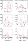 |
Fig. 1. Comparison between the data of Illustris-1 and Illustris-TNG100. The black lines mark the TNG data, while the red ones the Illustris-1 data. The solid line refers to the data at z = 0, while the dashed lines to the data at z = 4. From top left to bottom right we show: the effective radius Re (enclosing half the total luminosity or half the total stellar mass (for TNG); the effective surface brightness Ie; the central star velocity dispersion σ; the stellar mass-to-light ratio (M*/L); the total luminosity (in solar units); and the total stellar mass (in solar units). |
For both Illustris-1 and IllustrisTNG, we did not extract information on the morphology of the galaxies. For this reason, ETGs and late-type galaxies (LTGs) are mixed in our comparison plots. This choice originates from the observation that the SSRs of ETGs and LTGs are almost identical. This is clearly seen in Fig. 2, which shows the Re − M* (left panel) and the Ie − Re (right panel) for the ETGs (open circles) and LTGs (filled black circles). The two distributions are very closely superposed in both diagrams. The only exception is that very large Re are observed only for the most massive ETGs. This is only partially in agreement with Fig. 11 of Huertas-Company et al. (2019), which shows that ETGs and LTGs follow similar trends, but with small systematic differences for the two morphological types. The data of the WINGS database do not suggest any significant difference in the SSRs of LTGs and ETGs. We believe that the effective radii Re measured in the work of these latter authors are affected by a systematic bias due to the method used to derive Re. While for the WINGS galaxies, the effective radius was measured as the circle enclosing half the total luminosity, Huertas-Company et al. used the semi-major axis of the best-fitting Sérsic model. This choice likely introduces a systematic effect due to the inclination of the galaxies and the intrinsic shape of the light profiles. In any case, the inclusion of LTGs is a potential source of bias.
 |
Fig. 2. The Re − M* (left panel) and the Ie − Re (right panel) planes for the WINGS galaxy sample. LTGs (black dots) and ETGs (open circles) share the same distributions in these SSRs. The effective radius Re is given in kiloparsecs in the Re − M* plane and in parsecs in the Ie − Re plane. Masses are given in solar units. |
In addition, we note that the completeness of the samples is not critical for the conclusions drawn here. Indeed, we do not attempt any statistical analysis of the data, nor do we fit any distribution to derive correlations. The data are only used to qualitatively show how the distribution of galaxies in the various planes can change with the different cosmic epochs and how the L =  σβ law and the β parameter can at least qualitatively account for the variations expected or observed across time. The analysis carried out here is indeed somewhat independent of the level of precision reached by the models of the different sources, because we are mainly interested in presenting the method for deciphering the information encrypted in the observational data of the SSRs. The only hypothesis made here is that we can trust the results of simulations at high redshifts. This hypothesis is based on the fact that the simulations are able to reproduce some features of the distributions seen in the FP projections at redshifts z ∼ 0 and the tilt of the FP at z ∼ 1 (see below). The artificial galaxies match the observations relatively well, reproducing the position of the brightest cluster galaxies and the existence of the ZOE. All of the above gives us confidence that the simulations produce galaxies with luminosities, stellar masses, and effective radii that are not significantly different from those of real galaxies.
Figure 3 shows the four main important SSRs for the WINGS and Illustris data. The left upper panel shows stellar mass M* versus effective radius Re3. The WINGS data (black dots), the Illustris-1 data (red dots), and the IllustrisTNG data (blue dots) at z = 0 are well visible. We note that the Re − M* relation is clearly nonlinear. The galaxies of small mass are distributed almost horizontally, while the brightest galaxies follow a tail with a slope of close to 1. The real and simulated data nicely superimpose each other over the same range of mass, even if the effective radii provided by Illustris-1 for the least luminous galaxies are systematically greater than those observed. In contrast, IllustrisTNG gives much smaller radii for the low-mass galaxies, which we already discussed in the earlier papers of this series (see e.g., D’Onofrio et al. 2020; D’Onofrio & Chiosi 2022; D’Onofrio & Chiosi 2023). Both observations and simulations suggest the presence of the tail for the brightest ETGs, in which radii and masses are almost identical between observations and simulations. The different number of objects in the tail is due to the fact that different volumes are sampled and to the way in which the samples were created: the WINGS and Illustris-1 datasets include only objects from clusters of galaxies, where large ETGs are frequent, while IllustrisTNG takes galaxies from the general field. In addition, the total volume is different in each of the WINGS, Illustris-1 and IllustrisTNG surveys.
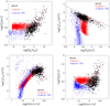 |
Fig. 3. The Re − M* plane and the three different projections of the FP. The black dots are the WINGS observational data. The red and blue dots are the data extracted from Illustris-1 and Illustris TNG-100, respectively. The galaxies with log(Re) < 2.5 are not plotted here in order to better show the bulk of the galaxy distribution. |
The upper right panel of Fig. 3 shows the Ie − Re plane obtained with the same data (here the sample of WINGS galaxies is much smaller than in Fig. 2 because only the subsample is involved). The important takeaway here is that the simulations correctly reproduce the presence of the tail for the brightest ETGs, which is clearly separated from the cloudy distribution of the least luminous galaxies. This tail, already seen in the original paper of Kormendy (1977), has a slope of close to −1 (that predicted by the VT) and has been attributed to the peculiar evolution of the brightest galaxies, which grow in mass by minor mergers (among others, see e.g., Capaccioli et al. 1992). Our conclusion is therefore that both simulations catch the presence of some peculiar features of the Ie − Re plane: the cloudy distribution of the faint galaxies, the tail formed by the brightest ETGs, and the ZoE, that is, the region totally void of galaxies above the dashed black line in Fig. 2.
The lower panels of Fig. 3 show the other projections of the FP: the Ie − σ and Re − σ planes. Again, we observe that the data points of the two simulations overlap the observational data relatively closely. In particular, the simulations are able to reproduce the curvature observed in the two distributions.
The good agreement between observations and simulations at z = 0 is a good starting point; it tells us that simulations are able to reproduce the main features of the SSRs at z = 0. However, given that our aim is to use simulations to infer the possible behavior of the SSRs at higher cosmic epochs, we need further proof that simulations are able to catch the structural parameters of galaxies at much higher redshifts. To this end, we used the data of di Serego Alighieri et al. (2005), who analyzed the FP at z ∼ 1. In our Fig. 4, we can appreciate that the FP at this redshift epoch coming from the Illustris data (red and blue circles as before) is in good agreement with the observed FP (black filled circles). The tilt of the plane is identical to a value for the a coefficient a bit lower than 1 (for the Coma cluster, the tilt is a ∼ 1.2). The tilt is different with respect to that measured for the local clusters and this is an indication that there is an evolution of the structural parameters that seems to be reproduced by the simulations. Even in this case, we note that the radii of the galaxies in the simulations are slightly systematically larger than those measured for the real galaxies, but this does not change the FP tilt of the simulated galaxies. Given that the total luminosity of the galaxies is relatively well reproduced by the simulations, the combination of Ie and Re is likely correct and the different effective radius simply changes Ie in such a way that the galaxy shifts along the FP and not orthogonally to it.
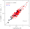 |
Fig. 4. Fundamental plane at redshift z = 1. The black filled circles are the data of di Serego Alighieri et al. (2005). The red and blue circles are the data from Illutris-1 and IllustrisTNG, respectively. The FP was determined considering only the galaxies with masses in the same range as those of the observational sample (those with M* > 1010 M⊙). |
In conclusion, we observe that the artificial galaxies in the simulations are in relatively good agreement with the real galaxies for what concerns the main structural parameters, even at much larger redshifts. The main differences with real galaxies are in terms of stellar content, colors, and SFR, but these differences are not so strong to generate weird distributions in the SSRs. For this reason, we believe that it is possible to extract information on the evolution of galaxies by looking at the distributions of galaxies in the SSRs. When high-redshift data become available in significant quantities, we will be able to better compare observations and simulations and extract useful information on the evolution of galaxies.
3. The basic equations of our framework
Before discussing the main SSRs predicted for furthest cosmic epochs, it is important to summarize the main conclusions drawn by D’Onofrio & Chiosi (2022, 2023) based on the combination of VT and the L =  σβ law4. This combination is the key novelty of the approach of these authors and understanding the main premise is necessary in order to be able to interpret the results presented in the following sections. The two equations representing VT and the L =
  σβ law are:
 (2)
(2)
In these equations, β and  are free time-dependent parameters that depend on the particular history of each object. From these equations, we can derive all the mutual relationships existing among the parameters characterizing a galaxy; namely Ms, Re, L, Ie, and σ. We find:
 (3)
(3)
for the Ie − Re plane, where
and Π is a factor that depends on kv, M/L, β, and  , and is given by
![Mathematical equation: $$ \begin{aligned}&\Pi = \left[ \left(\frac{2\pi }{L^\prime _0}\right)^{1/\beta } \left(\frac{L}{M_{\rm s}} \right)^{(1/2)} \left(\frac{k_{v}}{2\pi G} \right)^{(1/2)} \right]^{\frac{1}{1/2-1/\beta }}. \end{aligned} $$](/articles/aa/full_html/2023/07/aa45940-23/aa45940-23-eq22.gif)
We then have
![Mathematical equation: $$ \begin{aligned} I_{\rm e} = \left[ \frac{G}{k_{v}}\frac{L^\prime _0}{2\pi }M_{\rm s} \Pi ^{3/\gamma } \right]^{\frac{\beta -2}{1+3/\gamma }} \sigma ^{\frac{\beta -2}{1+3/\gamma }} \end{aligned} $$](/articles/aa/full_html/2023/07/aa45940-23/aa45940-23-eq23.gif) (4)
(4)
for the Ie − σ relation and
![Mathematical equation: $$ \begin{aligned} R_{\rm e} = \left[ \frac{G}{k_{v}}\frac{L^\prime _0}{2\pi }\frac{M_{\rm s}}{\Pi } \right] \sigma ^{\frac{\beta -2}{3+\gamma }} \end{aligned} $$](/articles/aa/full_html/2023/07/aa45940-23/aa45940-23-eq24.gif) (5)
(5)
for the Re − σ relation. In addition, we have
![Mathematical equation: $$ \begin{aligned} R_{\rm e} = \left[\left(\frac{G}{k_{v}}\right)^{\beta /2} \frac{L^\prime _0}{2\pi } \frac{1}{\Pi } \right]^{\frac{2(\beta -2)}{\beta ^2-6\beta +12}} M_{s}^{\frac{\beta ^2-2\beta }{\beta ^2-6\beta +12}} \end{aligned} $$](/articles/aa/full_html/2023/07/aa45940-23/aa45940-23-eq25.gif) (6)
(6)
for the Re − M* relation.
It is important to note here that, in all these equations, the slopes of the log relations depend only on β. This means that when a galaxy changes its luminosity L and its velocity dispersion σ, that is, when β has a well-defined value (either positive or negative), the effects of the motion in the L − σ plane are propagated in all the FP projections. In these planes, the galaxies cannot move in all directions, but are forced to move along the directions (slopes) predicted by the β parameter in the above equations. In this sense, the β parameter is the link we are looking for between the FJ (and the FP) and the observed distributions in the FP projections.
In addition, the combination of Eq. (2) gives us another important equation. It is now possible to write an FP-like equation that is valid for each galaxy depending on the β and  parameters:
 (7)
(7)
where the coefficients
 (8)
(8)
are written in terms of β and  . We note that this is the equation of a plane whose slope depends on β and the zero-point on
  . The similarity with the FP equation is clear. The novelty is that the FP is an equation derived from the fit of a distribution of real objects, while here each galaxy independently follows an equation that is formally identical to the classical FP but is of profoundly different physical meaning. In this case, as β and
  are time dependent, the equation represents the instantaneous plane on which a generic galaxy is located in the log(σ)−log(Ie)−log(Re) space and consequently in all its projections.
Finally, the combination of the above equations allows us to determine the values of β and  , the two critical evolutionary parameters. This is possible by writing the following equations:
![Mathematical equation: $$ \begin{aligned}&\beta [\log (I_{\rm e})+\log (G/k_{v})+\log (M_{\rm s}/L)+\log (2\pi )+\log (R_{\rm e})] + \\ \nonumber&\qquad \qquad + 2\log (L^\prime _0) - 2\log (2\pi ) - 4\log (R_{\rm e}) = 0 \end{aligned} $$](/articles/aa/full_html/2023/07/aa45940-23/aa45940-23-eq33.gif) (9)
(9)
 (10)
(10)
Posing now:
 (11)
(11)
we obtain the following system:
 (12)
(12)
 (13)
(13)
with solutions:
 (14)
(14)
 (15)
(15)
The key result here is that the parameters L, Ms, Re, Ie, and σ of a galaxy fully determine the evolution that is encoded in the parameters β and  .
.
Considering the fact that each structural parameter is known with a maximum error of ∼20%, we cannot fully rely on the single values of beta. On average, we instead show that the galaxies move in the SSRs only in the directions defined by beta. Given this premise, we proceed now to show the basic SSRs at much higher redshifts.
4. The SSRs at high redshift
To explore the behavior of the SSRs at high redshifts, we can only relay on simulations because we do not have enough observational data for galaxies at high redshift. Fortunately, despite the small systematic overestimate of the effective radii, the Illustris-1 and IllustrisTNG data are sufficiently precise to be trusted even at high redshifts. Furthermore, as shown by D’Onofrio & Chiosi (2023), both Illustris-1 and IllustrisTNG produce a very similar distribution for the β parameter. Thanks to this, the simulated data can provide reliable insight into the evolution of the SSRs with time. In the following, we show the results for both the Illustris-1 and IllustrisTNG samples currently available to us.
Figures 5 and 6 present the Ie − Re plane from z = 4 (upper left) to z = 0 (bottom right) for the Illustris-1 and IllustrisTNG, respectively. For Illustris-1, the whole sequence of redshifts is z = 4 (left upper panel), z = 3, z = 2.2, z = 1.6, z = 1.0, z = 0.6, z = 0.2, and z = 0 (right bottom panel) as indicated. In all the panels, the colored dots indicate galaxies with β > 0 and the black points those with β < 0. Crosses and open squares indicate galaxies with SFR greater than the average ⟨SFR⟩ or lower than the average, respectively, at each redshift epoch. The same color code is also used for the arrows indicating the mean slope of β, which was calculated from Eq. (15) for each object of the simulation. This mean value provides approximately the direction of motion in this plane for most of the galaxies, as expected from Eq. (3).
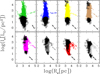 |
Fig. 5. The Ie − Re plane at different redshift for Illutris-1. From top left to bottom right, we can see the distribution of galaxies at z = 4, z = 3, z = 2.2, z = 1.6, z = 1.0, z = 0.6, z = 0.2, and z = 0. The colored dots mark the galaxies with β > 0 at each epoch, whereas the black symbols mark those with β ≤ 0. The crosses mark the galaxies with SFR greater than the mean ⟨SFR⟩ at each epoch, while the open squares show those with SFR lower than ⟨SFR⟩. The arrows indicate the average direction of motion predicted on the basis of the values of β from Eq. (3); see also Table 1. The colored arrows mark the average for the galaxies with β > 0 and the black arrows those with β ≤ 0. Their length is not related or proportional to any other quantity; it was chosen for graphical reasons. |
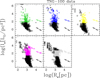 |
Fig. 6. The Ie − Re plane at different redshift for the TNG-100 data. From top left to bottom right, we show the distribution of galaxies at z = 4, z = 3, z = 2.2, z = 1.0, and z = 0. The colored dots mark the galaxies with β > 0 at each epoch, whereas the black symbols mark those with β ≤ 0. The crosses mark the galaxies with SFR greater than the mean ⟨SFR⟩ at each epoch, while the open squares show those with SFR lower than ⟨SFR⟩. The arrows indicate the average direction of motion predicted on the basis of the values of β from Eq. (3); see also Table 1. The colored arrows mark the average for the galaxies with β > 0 and the black arrows show those with β ≤ 0. Their length is not related or proportional to any other quantity; it was chosen for graphical reasons. |
The sequence of panels indicates that the tails well visible at z = 0 for the brightest galaxies start to appear at z ∼ 1 − 1.5. This epoch probably corresponds to the time in which minor mergers either with or without star formation on already formed massive objects became the typical event, thus increasing both the mass and radius of galaxies (Naab et al. 2009). It is interesting to note that the directions of the arrows, whose slope depends on Eq. (3) (see Table 1), flip progressively with z, in particular for positive β values, assuming the value close to −1 (as predicted by the VT) at approximately z = 0.6, and remain constant thereafter. This slope gives the only possible direction of motion of galaxies in the Ie − Re plane at each epoch when the evolution proceeds and β changes. The brightest galaxies, which likely reached full virial equilibrium far back in the past, are no longer affected by strong episodes of star formation, and start to move along this direction at z ∼ 1 − 1.5, forming the tail we observe today. Notably, even the galaxies with β ≤ 0 progressively reach the same slope. This happens because several objects have large negative β values. As we show below, both positive and negative values of β are possible and, as demonstrated by D’Onofrio & Chiosi (2021), this is a necessary condition for reproducing the L − σ distribution starting from the Ie − Re distribution (and vice versa).
Slopes of the Ie − Re, Re − σ, Ie − σ, and Re − M* planes for different values of β.
A further notable finding is that the galaxies with strong SFR (greater than ⟨SFR⟩) have in general a positive β. When an object with negative β appears on top of the distribution, it has a SFR that is greater than ⟨SFR⟩. Only later on, when the present epoch is approached, we start to see galaxies in the upper part of the cloud with negative β and a lower SFR than ⟨SFR⟩ (the black open squares). These objects might be relatively small compact galaxies where star formation has finished (a possible candidate for this class of galaxies could be M32). Notably, the galaxies with the higher surface brightness have positive β at high redshift and only later is this region of the plot populated by objects with negative β and low SFR.
A very similar behavior is observed in Fig. 6 when we use the IllustrisTNG data. As in Fig. 5, the colored dots indicate the galaxies with positive β and the arrows show the mean value of β. With respect to the previous figure, we note that the colored arrows show fewer changes of direction. We attribute this behavior to the different dimensions of the two samples. For the Illutris-TNG data, the arrows always have a slope of close to −1, a fact that indicates the relatively large values for β. In any case, the trend of populating the upper region of high surface brightness with objects with negative β and low ⟨SFR⟩ is confirmed.
One might now ask wonder what it is that produces the tail for the brightest objects in the Ie − Re plane, as the arrows at all redshift epochs are directed in approximately the same directions. This can be better understood by looking at the other FP projections and taking into account that the physical mechanisms at work in small and large galaxies can be different.
Figure 7 provides a better demonstration of how the changes of β across time determine the motions in the FP projections (the symbols and color code have the same meaning as those in Fig. 5). In the Ie − σ plane, the curvature formed by the brightest galaxies is much more pronounced. We note again that as β increases, the colored arrows point in the direction of the tail that we see at z ∼ 0. In the figure, we also note that the galaxies with negative β are preferentially at the bottom of the cloud distribution and their number decreases up to z ∼ 0.6 − 1.0. They then increase again in number and tend to crowd the top region of the distribution. As before, the upper region of the distribution with high Ie is populated by objects with high SFR at the most remote epochs, and only when approaching z = 0 do galaxies with negative β and low SFR appear on top of the distribution.
Again, the TNG data (Fig. 8) suggest a similar picture for the Ie − σ plane. With these data, the change of direction due to positive and negative values of β is much more evident and we understand that the tail originates when β increases and the galaxies progressively become much virialized.
Figures 9 and 10 display the Re − σ plane with the Illutris-1 and Illutris-TNG data, respectively. Again the slopes of the arrows predicted by Eqs. (3)–(5) are in good agreement with those inferred from the observed distribution of real galaxies and explain the tail formed by the bright galaxies. The same can be said for the Re − M* plane (Figs. 11 and 12). In both planes, the tail formed by the brightest galaxies stands out clearly. The slope of the tail in the Re − M* plane is very close to 1, as predicted by VT. The bottom right panel (at z = 0) shows in particular that objects with large negative or positive values of β begin to climb the tail as soon as their mass exceeds about 1011 M⊙.
As in the Ie − Re plane, the TNG data exhibit relatively similar mean values for the slopes predicted at the different redshifts. The slope is close to 1 and this means that the majority of the galaxies are relatively well virialized at z = 0. A further notable finding is that the TNG100 data indicate the presence of relatively massive objects with small radii that are not visible in Illustris-1. These objects might be the class of compact massive galaxies with high Ie also visible in Figs. 6 and 8. Notably, we can see that all these objects have negative β and very low SFR; in other words, they are isolated compact massive galaxies where the SF stopped a long time ago.
The picture we illustrate here using the Illustris-1 and Illutris-TNG data clearly reveals a progressive trend in the galaxies toward the full virial equilibrium, as indicated by the slopes of the arrows when |β|→∞. This condition is reached by the most massive galaxies at approximately z = 1.5 − 1.0. In general, the galaxies with the largest radii have β > 0, both in simulations and observations. This behavior is compatible with the predictions of minor mergers in which galaxies might increase their radius without significantly changing their mass or luminosity (Naab et al. 2009; Genel et al. 2018).
Finally, we note that the FJ relation does not change significantly with redshift. As the redshift decreases from z = 4 to z = 0 through six intermediate steps, we observe that some galaxies have negative β and others have positive β. The fits of the observed distributions reveal that the slope of the FJ relation progressively decreases, passing from nearly 4 (at z = 4) to nearly 2 (at z = 0).
One may legitimately ask why the scatter of the FJ relation does not increase with time, given that there are objects that move almost perpendicularly to the trend indicated by the observed distribution. The same trend is visible with the TNG data (not plotted here). We believe that the scatter cannot increase as a consequence of the merger activity because the maximum possible variation in luminosity that a galaxy might experience does not exceed a factor of two (when a galaxy approximately doubles its mass by merging with a similar object of the same mass and stellar content), which in log units corresponds to a factor of ∼0.3, a very small shift compared with the scale spanned by the data values.
To support this statement, in Appendix A we present a toy model predicting the changes that a galaxy with a mass M1, age T1, and luminosity L1 would undergo in terms of total luminosity as a consequence of a merger with another object of mass M2, age T2, and luminosity L2. The event may or may not be followed by star formation engaging a certain amount of gas with mass M3.
Using reasonable values for the masses and luminosities of the three components (see Eq. (A.5) in Appendix A), we may expect that the total luminosity first increases and then decreases on a timescale that depends on the amount of matter engaged in the burst of activity. In any case, the luminosity evolution is fast up to a few 108 years after the burst (turnoff mass about 3 M⊙), slows down up to 109 years (turnoff mass of about 2 M⊙), and then becomes even slower afterwards. The estimated fading rate of the luminosity is about |Δ(log L/L⊙)| ≃ 0.015 per gigayear (Gyr) and per unit SSP mass, which must be multiplied by 5.8 to get the real fading rate per Gyr (see the SSP database of Tantalo 2005). Consequently, it is very unlikely to catch a galaxy exactly at the time of maximum luminosity. Equation (A.5) allows us to quickly evaluate the effects of mergers with different combinations of masses and ages of the involved galaxies. However, the examples shown in Appendix A demonstrate that, except for the case of a merger between two objects of comparable mass, in which the luminosity and mass of the resulting objects are double the original ones, mergers among objects of different mass and age, and likely undergoing some star formation during the merger, generate objects that do not keep traces of the merger but simply keep the properties (mass and luminosity) of the most massive component. More details are not of interest here.
The main conclusion of this section of our study can be summarized as follows. The hypothesis that VT and the relation of L =  σβ work together to govern the evolution of mass Ms, luminosity L, radius Re, surface brightness Ie, and velocity dispersion σ leads to a coherent and self-consistent explanation of all the scale relations of galaxies, and also provides a reasonable explanation for the tilt of the FP as demonstrated by D’Onofrio & Chiosi (2022, 2023).
5. The important role of β
In order to better understand the effects played by β, it is necessary to think about the possible variations of Re and Ie when L and σ vary in the L − σ plane. There are six possible changes of L and σ in this plane: σ either decreases, increases, or remains constant, and the same is true for L. The effective relationship between the two variables depends in turn on β; for example, when β is negative, there is not necessarily a decrease in luminosity, and when β is positive, a decrease in luminosity might also occur (see D’Onofrio & Chiosi 2022; D’Onofrio & Chiosi 2023, for a detailed discussion of this topic). The ambiguity in the direction of evolution can only be solved by looking at the movements of the galaxies in the different SSRs, and in particular by observing the behavior of Ie. When the luminosity of a galaxy changes, both the effective radius Re and the mean effective surface intensity Ie vary. This happens because Re is not a true physical radius, similarly to the virial radius for example (which depends only on the total mass), but it is the radius of the circle that encloses half the total luminosity of the galaxy. As galaxies have different stellar populations with different ages and metallicity, it is very unlikely that a change in luminosity would not change the whole shape of the luminosity profile and therefore the value of Re. If the luminosity decreases passively, in general one could expect a decrease in Re and an increase in Ie. On the other hand, if a shock induced by harassment or stripping induces an increase in L (and a small decrease in σ), we might expect an increase in Re and a decrease in Ie. The observed variations of these parameters depend strongly on the type of event that a galaxy is experiencing (stripping, shocks, feedback, merging, etc.). In general, one should keep in mind that these three variables L, Re and Ie are strongly coupled to each other and that even a small variation in L might result in ample changes of Re and Ie.
In summary, as already pointed out, the variations of the parameter β with time are responsible of all the changes observed in the FP projections. This means that the FP problem should be considered from an evolutionary point of view, where time plays an important role and the effects of evolution are visible in all the FP projections. The single SSRs are snapshots of an evolving situation. The L =  σβ law is informative of this kind of evolution, and can be used to predict the correct direction of motion of each galaxy in the basic diagnostic planes.
We now show that the parameter β changes with the cosmic epochs and that such variations are in turn related mainly to the change of the mean surface intensity due to the natural variation of the star formation activity with time. We show that β tends to be low when star formation is high and vice versa. However, large scatter is seen at all epochs. Furthermore, we show that β increases considerably if and when the galaxy attains the condition of full virialization, that is, when the two variables Ms and Re combine in such a way as to yield the measured velocity dispersion (i.e., that measured for the stellar content).
Figure 13 shows the β − log(Ie) plane. The dots of different colors represent the galaxies at different redshifts using the same color code as in Fig. 5. From this plot, it is clear that β increases and log(Ie) on average decreases when the cosmic epoch approaches z = 0 (light gray dots). In the remote epochs (z = 4) and up to z ∼ 1.5, we observe an almost linear dependence of β on Ie, in which β ranges from 0 to ∼20. This condition is an indication that, at these epochs, the galaxies are still far from full virialization. The real data of WINGS (black dots) are very precisely superposed over the simulation data, showing a large spread with large positive and negative values of β.
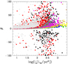 |
Fig. 13. The β − log(Ie) plane. The colored dots follow the same color code as in Fig. 5, marking the galaxies at different redshift epochs. The black dots are the data of the WINGS database at z = 0. |
This behavior of β is connected with the average SFR at the different cosmic epochs. This is clearly seen in Fig. 14, where we note that, when the SFR is high, the values of β are close to 0–10. The large scatter in β starts to be visible with the gray dots at z ∼ 0.6 − 1.0, the same epoch in which we see the tail of high-luminosity galaxies in the SSRs for the first time. Figure 15 also shows that β takes large positive and negative values preferably in galaxies with masses higher than ∼1010 M⊙.
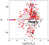 |
Fig. 15. The β − log(Ms) (stellar mass) plane. The color code and symbols are the same as in previous figures. |
Finally, Fig. 16 shows β versus the quantity [log(2T)] − log(Ω)], which is a proxy for the virial condition, being the difference between the kinetic and potential energy of the stellar systems. The figure clearly indicates that |β| increases, while β can be either positive or negative when the difference between the two energies approaches zero5. We note that β remains very close to zero at high redshift. This means that the galaxies are still far from virial equilibrium. In contrast, at low redshifts, the peak of β falls in the intervals 0 to 20 (z = 1) and 0 to 50 (z = 0) with increasing spread toward both high positive and low negative values.
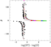 |
Fig. 16. The β − [log(2T)−log(Ω)] plane. The color code and symbols are the same as in previous figures. |
Figure 17 shows the histogram of the number frequency distribution (N/Ntot) of β in the model galaxies at different redshifts. There is not much difference between the histograms of the Illustris-1 and IllustrisTNG samples. The most remarkable features to note are that, (i) at high redshifts (z ≥ 2), the distribution peaks fall in the interval 4 ≤ β ≤ 0 with a small tail of positive values in the interval 0 ≤ β ≤ 4; (ii) the distribution gradually spreads to higher values of |β| at low redshifts (1 and 0), and both positive and negative values of β are present; and (iii) finally, at low redshifts the peaks are visible both in the positive and negative ranges of β values, and |β| can attain large values.
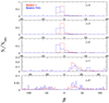 |
Fig. 17. Histogram of β for model galaxies of the Illustris-1 (red line) and IllustrisTNG (blue line) samples as a function of redshift. |
We observe this large dispersion in β because the term 1 − 2A′/A at the denominator of Eq. (15) becomes very close to zero. Consequently, both log( ) and β diverge. According to the direction from which this zero value is approached, one can have either very large and positive or large and negative values for β. As already discussed, this happens when the system is in conditions of strict virialization. The sign of β depends on the particular history of the variables Ms, Re, L, and Ie; in other words, whether the term 2A′/A is tending to 1 from below (β > 0) or above 1 (β < 0). From an operational point of view, we may define “state close to strict virialization” when |β|> 20.
Notably, the Illustris-1 and IllustrisTNG models agree very well with the observational data (black dots in these panels). The inclusion of real dynamics and the hierarchical scenario provides the necessary conditions to clearly demonstrate the action of virialization. The hierarchical scenario by mergers, ablation of stars and gas, harassment, secondary star formation, inflation of dimension by energy injections of various kinds, and so on induces strong variations of the fundamental parameters of a galaxy and hence strong temporary deviations from the virial conditions. However, after this happened, the viral conditions are soon recovered over a reasonable timescale, which can be short or long depending on the amount of mass engaged in the secondary star forming activity and the amount of time elapsed since the star forming event took place (see the burst experiments in Chiosi & Carraro 2002; Tantalo & Chiosi 2004). For this reason, detecting systems on their way back to virial equilibrium is likely a frequent event, which would explain the high dispersion seen on the β–Ie plane. The value of β evaluated for each galaxy can provide a useful hint as to the equilibrium state reached by the system. Most likely, the condition of strict virial equilibrium is a transient phenomenon that could occur several times during the life of a galaxy. This is suggested by the large number of galaxies with very small or very high β.
6. The history of mass assembly
The Illustris-1 and IllustrisTNG simulations have made clear that the history of the mass assembly of galaxies is not simple, but is characterized by repeated episodes of mass accretion and mass removal. Figures 18 and 19 show the main SSRs and the β − z plane, respectively. Eight single galaxies of different mass and evolutionary history extracted randomly from the sample are displayed in these plots. These galaxies are taken from our Illustris-1 sample. Each galaxy is indicated by a broken line of different color, while the mass assembly history of each object is represented by a series of dots of the same color. Along each line, there are eight points, one for each value of the redshift from z = 4 to z = 0 according to the list already presented in the previous sections. A very similar figure is obtained with the TNG data and these data are therefore not plotted here.
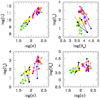 |
Fig. 18. The SSRs for eight single galaxies. The different colors mark the single galaxies. The positions in the diagram connected by the colored lines mark the distribution at different redshift epochs. |
The β values of these eight galaxies at different redshift are shown in Fig. 19 and are very close to zero at every epoch, with the exception of the blue track. The β values can be entered into Table 1 in order to derive the possible directions of motion at each redshift in each of the planes. For example, the yellow and green objects always have values of beta close to zero (slightly positive). These correspond to slopes of around ∼ − 2 in the Ie − Re plane, ∼2.5 in the Re − σ plane, and ∼ − 1.5 in the Ie − σ plane. These are therefore objects of the “big cloud” where galaxies can move in every possible direction. The blue galaxy on the other hand reaches relatively high values of β and it is possible to see that its movements are in the direction close to −1 in the Ie − Re plane.
It is clear from Fig. 18 that the galaxies do not move in the planes of the SSRs in a continuous and uniform way, but rather they randomly change their position at different epochs. In the same figure, we also note that the galaxies with blue, red, brown, and magenta colors are more massive, more luminous, and with higher σ than the others, even at early epochs (z = 4). More importantly, we emphasize that the same galaxies at epochs closer to the present day than z ∼ 1.5 are able to reach both large positive and negative values of β. Their βs start low and gradually increase, and may reach the state of virial equilibrium. In contrast, the less massive and fainter galaxies have always low βs (see Figs. 18 and 19) close to zero and are located in the region of low σ, Ie, and L. The dwarf galaxies never reach the condition of full virialization.
As already pointed out, the condition of full virial equilibrium can be a transient state in the sense that once reached, it cannot be maintained forever if a galaxy undergoes an event such as a merger, stripping, and/or harassment, which may push it away from this condition. However, virial equilibrium can be recovered again on a suitable timescale, which depends on the relative intensity of the disturbing event. For instance, in the case of a merger between two galaxies of comparable mass, which would most likely be accompanied by intense star formation, the resulting system will not be in virial equilibrium and will take a significant amount of time to reach this condition. On the contrary, the merger between two galaxies of significantly different mass, which is likely to be accompanied by modest star formation, will only slightly depart from the virial condition. If so, we expect that after a certain redshift, only the massive galaxies remain unperturbed by mergers and can move toward the condition of strict virialization, while the low-mass ones are still far from this ideal condition. The few objects displayed in Fig. 19 are typical examples of the above situations.
7. Discussion and conclusions
The aim of this paper is to show that combining VT with the L =  σβ relation (which is a proxy for evolution, in which β and
  vary from galaxy to galaxy and over the course of time) has many positive consequences (see D’Onofrio et al. 2017; D’Onofrio et al. 2019; D’Onofrio et al. 2020; D’Onofrio & Chiosi 2021, for earlier studies along this line of thought). The variation of β and
  with time traces the path followed by each galaxy in the various SSRs. The combination of the L =
  σβ law and VT yields Ie − Re, Re − σ, Ie − σ, and Re − M* relations that nicely reproduce the data and more important strongly suggest the existence of a system of two equations in the unknowns β and
  with coefficient functions of Ms, Re, L, and Ie. Importantly, for each galaxy, this system of equations can be used to determine the values of β and
  . With the aid of these relations, we can determine the instantaneous position and direction of motion of a galaxy on the FP and its projection planes. As these equations are limited to ETGs, we name them fundamental equations of galaxy structure and evolution (D’Onofrio & Chiosi 2022; D’Onofrio & Chiosi 2023).
With this study, we show that the Illustris-1 and IllustrisTNG databases provide the basic parameters of galaxies, and that these are in satisfactory agreement with those derived from observational data for the galaxies at z ≃ 0. The given structural parameters indeed reproduce some distinct features observed in the FP projections, such as the tail of the bright ETGs, the ZOE, and the clumps of low-mass objects.
Based on these simulated data, we look at the SSRs at different epochs (from redshift z = 0 up to redshift z = 4), and highlight their expected behavior. In summary, we show that:
-
The SSRs change with time;
-
The variations of the SSRs can be explained by the variation of the β parameter driving the L =
 (t)σβ(t) law;
 -
When β varies with time, a galaxy can move in the SSRs, but only in well-defined directions, which ultimately depend on β. These directions change with time and, toward z = 0, progressively acquire the slope exhibited by the most massive galaxies which lay along the tail of the bright ETGs at z = 0;
-
The parameter β can take both positive and negative values over time. We therefore suggest that the parameter β can be considered as a thermometer that gauges the virialization conditions. Moreover, β can be either large and positive or large and negative when the galaxies are close to virial equilibrium;
-
The only galaxies that can reach the virial state are those that became sufficiently massive (above 109 − 1010 M⊙) at high redshifts (z = 4). These are no longer disturbed by the merging events, which become rare events after z ∼ 1.5 and/or in any case are not influential in terms of changing the mass ratio between donor and accretor;
-
Finally, the L =
 σβ relation can be considered as an empirical way of catching the temporal evolution of galaxies. The values of β (and
  ) mirror the history of mass assembly and luminosity evolution of a galaxy.
The conclusion is that SSRs are full of astrophysical information about galaxy evolution.
The measured parameters for the real galaxies are always shown in our plots with black dots. For this reason, in each of the plots containing real observations, the number of galaxies is not always the same.
The symbols Ms and M* used in this work both refer to the total stellar mass in solar units.
From here on, we drop the time notation for simplicity.
The difference predicted by the VT is zero, but the calculated energies depend on Re, which is not exactly the virial radius.
Acknowledgments
M.D. thanks the Department of Physics and Astronomy of the Padua University for the financial support.
References
- Allanson, S. P., Hudson, M. J., Smith, R. J., & Lucey, J. R. 2009, ApJ, 702, 1275 [NASA ADS] [CrossRef] [Google Scholar]
- Auger, M. W., Treu, T., Bolton, A. S., et al. 2010, ApJ, 724, 511 [NASA ADS] [CrossRef] [Google Scholar]
- Beifiori, A., Mendel, J. T., Chan, J. C. C., et al. 2017, ApJ, 846, 120 [NASA ADS] [CrossRef] [Google Scholar]
- Bernardi, M., Sheth, R. K., Annis, J., et al. 2003, ApJ, 125, 1866 [CrossRef] [Google Scholar]
- Bertelli, G., Bressan, A., Chiosi, C., Fagotto, F., & Nasi, E. 1994, A&AS, 106, 275 [NASA ADS] [Google Scholar]
- Bertelli, G., Girardi, L., Marigo, P., & Nasi, E. 2008, A&A, 484, 815 [NASA ADS] [CrossRef] [EDP Sciences] [Google Scholar]
- Biviano, A., Moretti, A., Paccagnella, A., et al. 2017, A&A, 607, A81 [NASA ADS] [CrossRef] [EDP Sciences] [Google Scholar]
- Bolton, A. S., Burles, S., Treu, T., Koopmans, L. V. E., & Moustakas, L. A. 2007, ApJ, 665, L105 [NASA ADS] [CrossRef] [Google Scholar]
- Bolton, A. S., Treu, T., Koopmans, L. V. E., et al. 2008, ApJ, 684, 248 [NASA ADS] [CrossRef] [Google Scholar]
- Borriello, A., Salucci, P., & Danese, L. 2003, MNRAS, 341, 1109 [NASA ADS] [CrossRef] [Google Scholar]
- Bottrell, C., Torrey, P., Simard, L., & Ellison, S. L. 2017, MNRAS, 467, 2879 [NASA ADS] [CrossRef] [Google Scholar]
- Busarello, G., Lanzoni, B., Capaccioli, M., et al. 1998, Mem. Soc. Astron. It., 69, 217 [NASA ADS] [Google Scholar]
- Capaccioli, M., Caon, N., & D’Onofrio, M. 1992, MNRAS, 259, 323 [NASA ADS] [CrossRef] [Google Scholar]
- Cappellari, M., Bacon, R., Bureau, M., et al. 2006, MNRAS, 366, 1126 [Google Scholar]
- Cariddi, S., D’Onofrio, M., Fasano, G., et al. 2018, A&A, 609, A133 [NASA ADS] [CrossRef] [EDP Sciences] [Google Scholar]
- Cava, A., Bettoni, D., Poggianti, B. M., et al. 2009, A&A, 495, 707 [NASA ADS] [CrossRef] [EDP Sciences] [Google Scholar]
- Chiosi, C., & Carraro, G. 2002, MNRAS, 335, 335 [NASA ADS] [CrossRef] [Google Scholar]
- Chiosi, C., Bressan, A., Portinari, L., & Tantalo, R. 1998, A&A, 339, 355 [NASA ADS] [Google Scholar]
- Ciotti, L. 1991, A&A, 249, 99 [NASA ADS] [Google Scholar]
- Ciotti, L., Lanzoni, B., & Renzini, A. 1996, MNRAS, 282, 1 [Google Scholar]
- Courteau, S., Faber, S. M., Dressler, A., & Willick, J. A. 1993, ApJ, 412, L51 [NASA ADS] [CrossRef] [Google Scholar]
- de Carvalho, R. R., & Djorgovski, S. 1992, ApJ, 389, L49 [NASA ADS] [CrossRef] [Google Scholar]
- de Graaff, A., Bezanson, R., Franx, M., et al. 2021, ApJ, 913, 103 [CrossRef] [Google Scholar]
- di Serego Alighieri, S., Vernet, J., Cimatti, A., et al. 2005, A&A, 442, 125 [NASA ADS] [CrossRef] [EDP Sciences] [Google Scholar]
- Djorgovski, S., & Davis, M. 1987, ApJ, 313, 59 [Google Scholar]
- D’Onofrio, M., & Chiosi, C. 2021, Universe, 8, 8 [CrossRef] [Google Scholar]
- D’Onofrio, M., & Chiosi, C. 2022, A&A, 661, A150 [NASA ADS] [CrossRef] [EDP Sciences] [Google Scholar]
- D’Onofrio, M., & Chiosi, C. 2023, A&A, submitted [Google Scholar]
- D’Onofrio, M., Valentinuzzi, T., Secco, L., Caimmi, R., & Bindoni, D. 2006, New A Rv., 50, 447 [CrossRef] [Google Scholar]
- D’Onofrio, M., Fasano, G., Varela, J., et al. 2008, ApJ, 685, 875 [CrossRef] [Google Scholar]
- D’Onofrio, M., Bindoni, D., Fasano, G., et al. 2014, A&A, 572, A87 [NASA ADS] [CrossRef] [EDP Sciences] [Google Scholar]
- D’Onofrio, M., Cariddi, S., Chiosi, C., Chiosi, E., & Marziani, P. 2017, ApJ, 838, 163 [CrossRef] [Google Scholar]
- D’Onofrio, M., Sciarratta, M., Cariddi, S., Marziani, P., & Chiosi, C. 2019, ApJ, 875, 103 [Google Scholar]
- D’Onofrio, M., Chiosi, C., Sciarratta, M., & Marziani, P. 2020, A&A, 641, A94 [NASA ADS] [CrossRef] [EDP Sciences] [Google Scholar]
- Dressler, A. 1987, ApJ, 317, 1 [NASA ADS] [CrossRef] [Google Scholar]
- Dressler, A., & Faber, S. M. 1990, ApJ, 354, 13 [NASA ADS] [CrossRef] [Google Scholar]
- Dressler, A., Lynden-Bell, D., Burstein, D., et al. 1987, ApJ, 313, 42 [Google Scholar]
- Faber, S. M., & Jackson, R. E. 1976, ApJ, 204, 668 [Google Scholar]
- Faber, S. M., Dressler, A., Davies, R. L., et al. 1987, in Nearly Normal Galaxies. From the Planck Time to the Present, 175 [Google Scholar]
- Fasano, G., Marmo, C., Varela, J., et al. 2006, A&A, 445, 805 [NASA ADS] [CrossRef] [EDP Sciences] [Google Scholar]
- Fasano, G., Vanzella, E., Dressler, A., et al. 2012, MNRAS, 420, 926 [Google Scholar]
- Forbes, D. A., Ponman, T. J., & Brown, R. J. N. 1998, ApJ, 508, L43 [NASA ADS] [CrossRef] [Google Scholar]
- Franx, M., van Dokkum, P. G., Förster Schreiber, N. M., et al. 2008, ApJ, 688, 770 [NASA ADS] [CrossRef] [Google Scholar]
- Fritz, J., Poggianti, B. M., Bettoni, D., et al. 2007, A&A, 470, 137 [NASA ADS] [CrossRef] [EDP Sciences] [Google Scholar]
- Genel, S., Vogelsberger, M., Springel, V., et al. 2014, MNRAS, 445, 175 [Google Scholar]
- Genel, S., Nelson, D., Pillepich, A., et al. 2018, MNRAS, 474, 3976 [Google Scholar]
- Girardi, L., Bressan, A., Chiosi, C., Bertelli, G., & Nasi, E. 1996, A&AS, 117, 113 [NASA ADS] [CrossRef] [EDP Sciences] [Google Scholar]
- Gregg, M. D. 1992, ApJ, 384, 43 [NASA ADS] [CrossRef] [Google Scholar]
- Gullieuszik, M., Poggianti, B., Fasano, G., et al. 2015, A&A, 581, A41 [NASA ADS] [CrossRef] [EDP Sciences] [Google Scholar]
- Guzman, R., Lucey, J. R., & Bower, R. G. 1993, MNRAS, 265, 731 [NASA ADS] [CrossRef] [Google Scholar]
- Holden, B. P., van der Wel, A., Kelson, D. D., Franx, M., & Illingworth, G. D. 2010, ApJ, 724, 714 [NASA ADS] [CrossRef] [Google Scholar]
- Huertas-Company, M., Rodriguez-Gomez, V., Nelson, D., et al. 2019, MNRAS, 489, 1859 [NASA ADS] [CrossRef] [Google Scholar]
- Ibarra-Medel, H. J., & López-Cruz, O. 2011, Rev. Mex. Astron. Astrofis. Conf. Ser., 40, 64 [NASA ADS] [Google Scholar]
- Jorgensen, I., Franx, M., & Kjaergaard, P. 1996, MNRAS, 280, 167 [Google Scholar]
- Kormendy, J. 1977, ApJ, 218, 333 [NASA ADS] [CrossRef] [Google Scholar]
- La Barbera, F., Lopes, P. A. A., de Carvalho, R. R., de La Rosa, I. G., & Berlind, A. A. 2010, MNRAS, 408, 1361 [NASA ADS] [CrossRef] [Google Scholar]
- Lucey, J. R., Bower, R. G., & Ellis, R. S. 1991, MNRAS, 249, 755 [NASA ADS] [Google Scholar]
- Magoulas, C., Springob, C. M., Colless, M., et al. 2012, MNRAS, 427, 245 [NASA ADS] [CrossRef] [Google Scholar]
- Moretti, A., Poggianti, B. M., Fasano, G., et al. 2014, A&A, 564, A138 [NASA ADS] [CrossRef] [EDP Sciences] [Google Scholar]
- Moretti, A., Gullieuszik, M., Poggianti, B., et al. 2017, A&A, 599, A81 [NASA ADS] [CrossRef] [EDP Sciences] [Google Scholar]
- Naab, T., Johansson, P. H., & Ostriker, J. P. 2009, ApJ, 699, L178 [Google Scholar]
- Nasi, E., Bertelli, G., Girardi, L., & Marigo, P. 2008, Mem. Soc. Astron. It., 79, 738 [NASA ADS] [Google Scholar]
- Nelson, D., Pillepich, A., Genel, S., et al. 2015, Astron. Comput., 13, 12 [Google Scholar]
- Nelson, D., Pillepich, A., Springel, V., et al. 2018, MNRAS, 475, 624 [Google Scholar]
- Nipoti, C., Londrillo, P., & Ciotti, L. 2003, MNRAS, 342, 501 [Google Scholar]
- Novak, G. S. 2008, Ph.D. Thesis, University of California, Santa Cruz [Google Scholar]
- Oldham, L., Auger, M., Fassnacht, C. D., et al. 2017, MNRAS, 470, 3497 [CrossRef] [Google Scholar]
- Pahre, M. A., Djorgovski, S. G., & de Carvalho, R. R. 1996, ApJ, 456, L79 [NASA ADS] [CrossRef] [Google Scholar]
- Pillepich, A., Springel, V., Nelson, D., et al. 2018a, MNRAS, 473, 4077 [Google Scholar]
- Pillepich, A., Nelson, D., Hernquist, L., et al. 2018b, MNRAS, 475, 648 [Google Scholar]
- Prugniel, P., & Simien, F. 1996, A&A, 309, 749 [NASA ADS] [Google Scholar]
- Prugniel, P., & Simien, F. 1997, A&A, 321, 111 [NASA ADS] [Google Scholar]
- Reda, F. M., Forbes, D. A., & Hau, G. K. T. 2005, MNRAS, 360, 693 [NASA ADS] [CrossRef] [Google Scholar]
- Renzini, A., & Ciotti, L. 1993, ApJ, 416, L49 [NASA ADS] [CrossRef] [Google Scholar]
- Robertson, B., Cox, T. J., Hernquist, L., et al. 2006, ApJ, 641, 21 [NASA ADS] [CrossRef] [Google Scholar]
- Rodriguez-Gomez, V., Snyder, G. F., Lotz, J. M., et al. 2019, MNRAS, 483, 4140 [NASA ADS] [CrossRef] [Google Scholar]
- Samir, R. M., Reda, F. M., Shaker, A. A., Osman, A. M. I., & Amin, M. Y. 2016, NRIAG J. Astron. Geophys., 5, 277 [NASA ADS] [CrossRef] [Google Scholar]
- Snyder, G. F., Torrey, P., Lotz, J. M., et al. 2015, MNRAS, 454, 1886 [NASA ADS] [CrossRef] [Google Scholar]
- Springel, V., Pakmor, R., Pillepich, A., et al. 2018, MNRAS, 475, 676 [Google Scholar]
- Tantalo, R. 2005, in The Initial Mass Function 50 Years Later, eds. E. Corbelli, F. Palla, & H. Zinnecker, Astrophys. Space Sci. Libr., 327, 235 [NASA ADS] [CrossRef] [Google Scholar]
- Tantalo, R., & Chiosi, C. 2004, MNRAS, 353, 917 [NASA ADS] [CrossRef] [Google Scholar]
- Taranu, D., Dubinski, J., & Yee, H. K. C. 2015, ApJ, 803, 78 [Google Scholar]
- Tortora, C., Napolitano, N. R., Romanowsky, A. J., Capaccioli, M., & Covone, G. 2009, MNRAS, 396, 1132 [NASA ADS] [CrossRef] [Google Scholar]
- Trujillo, I., Burkert, A., & Bell, E. F. 2004, ApJ, 600, L39 [Google Scholar]
- Valentinuzzi, T., Woods, D., Fasano, G., et al. 2009, A&A, 501, 851 [NASA ADS] [CrossRef] [EDP Sciences] [Google Scholar]
- van Dokkum, P. G., & Franx, M. 1996, MNRAS, 281, 985 [NASA ADS] [CrossRef] [Google Scholar]
- van Dokkum, P. G., & van der Marel, R. P. 2007, ApJ, 655, 30 [NASA ADS] [CrossRef] [Google Scholar]
- Varela, J., D’Onofrio, M., Marmo, C., et al. 2009, A&A, 497, 667 [NASA ADS] [CrossRef] [EDP Sciences] [Google Scholar]
- Vogelsberger, M., Genel, S., Springel, V., et al. 2014a, Nature, 509, 177 [Google Scholar]
- Vogelsberger, M., Genel, S., Springel, V., et al. 2014b, MNRAS, 444, 1518 [Google Scholar]
Appendix A: Mergers and bursts of star formation
In order to better quantify the effect of a merger on the integrated light of a galaxy, we present here an elementary model of population synthesis. Let us consider two galaxies with total stellar mass M1 and M2 and total luminosity L1 and L2 (either bolometric or in some passband). The luminosity is generated by the stars already existing in each galaxy. The two galaxies are supposed to merge. The merger event may or may be not accompanied by star formation induced by the merger itself. Let M3 be the mass of gas (belonging to one of the galaxies or both) that is eventually turned into newly born stars. For simplicity, we consider this event as a unique single stellar population, SSP, of total mass M3, generating a total luminosity L3. If no star formation occurs at the merger M3 = 0 and L3 = 0.
The total mass of the system is
 (A.1)
(A.1)
and the ratios between the mass of each component and the total mass are
 (A.2)
(A.2)
(with no star formation M3 = 0). Let us suppose that the most massive object of the three is M1, followed by M2 and M3 (with M2 > M3). Therefore, we have the sequence α1 > α2 > α3.
The total luminosity is
 (A.3)
(A.3)
and the corresponding ratios between the luminosity of each component and the total luminosity are
 (A.4)
(A.4)
With no star formation, L3 = 0 and h3 = 0.
As the luminosity of a galaxy depends not only on the mass but also on the age (the luminosity gets fainter with increasing age) and it may undergo large and fast variations in the presence of star formation, the sequence h1 > h2 > h3 can be easily violated. It may be that h2 > h1 and h3 > h1 and/or h3 > h2. In summary, we define the following identities for the total mass and total luminosity, in which the contribution of each component is revealed:
 (A.5)
(A.5)
Given these premises, we briefly present the key ingredients of our analysis, namely the relation between the mass and luminosity of single stars and time. This provides clues as to the timescale over which the mass and light of the most massive objects in any generation of stars can vary with age. Each generation of stars forms a SSP with a certain abundance of chemical elements. In a SSP, stars are distributed in mass according to some initial mass function (IMF), in which the number of stars per mass interval typically increases with decreasing stellar mass; that is, many more faint stars of low mass than bright stars of high mass. As stars evolve and die, the total light emitted by a SSP decreases and the SSP becomes fainter and redder with time. Finally, galaxies are made of stars born at different epochs and dying at different times. Therefore, the stellar content of a galaxy can be conceived as a mixture of SSPs of different age, which therefore emit different amounts of light of different colors. The total light is the integral of the light emitted by each SSP weighted by the SFR over the whole history of a galaxy, all as a function of time and chemical composition.
In Fig. A.1, we show the time dependence of the mass (left panel) and luminosity (right panel) of single stars (lifetime and luminosity are taken at the stage of the brightest luminosity attained by the long-lived evolutionary stages) of different masses (in the interval 0.6 to 120 M⊙). In both panels, the colors indicate the metallicity and the ticks along each curve mark the value of the mass; blue is for low metal content and red for high metal content. Figure A.2 shows the luminosity versus time relationship for SSPs of different chemical composition as indicated (left panel), and model galaxies of different mass as indicated (right panel). The left panel shows the luminosity (in solar units) in the V-passband of the Johnson-Bessell system and of the SSPs with different metallicity (solid lines with different colors where blue is for low metal content and red for high metal content). The black solid line is the best fit of the luminosities for metallicities. In the same panel, and limited to the best fit, we also show the luminosity in the B-passband (dashed line). The right panel shows the V-luminosity in the same photometric system of model galaxies with infall over the entire lifetime of the galaxies. This is the luminosity integrated over the many generations of stars formed in the galaxy at a suitable SFR. Chemical enrichment of the gas from which the stars are formed is taken into account. Stellar models, SSPs, and model galaxies are taken from the Padua library of stellar models, isochrones, and SSPs (see Bertelli et al. 1994; Girardi et al. 1996; Bertelli et al. 2008; Nasi et al. 2008, for all details and ample referencing). The model galaxies were calculated by the authors and described in D’Onofrio & Chiosi (2023). The SSPs in use here are for the Salpeter IMF with a slope of x = 2.35 (in number of stars per mass interval), and the SSP mass and luminosity are named MSSP and LSSP with MSSP = 5.826 M⊙.
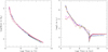 |
Fig. A.1. Stellar mass in M⊙ vs age in years (left panel). The asterisks along each curve are the star masses in the mass interval 0.6 to 120 M⊙. The color code of each curve indicates the chemical composition. Curves are also labeled in accordance with the mass abundance of metals Z according to the law ΔY/ΔZ = 2.5, where Y is the mass abundance of helium and the initial values are Z0 = 0.0001 and Y0 = 0.23. The values of the metalliciies are Z = 0.0001 (black), Z = 0.0004 (blue), Z = 0.004 (green), Z = 0.008 (magenta), Z = 0.020 (red), and Z = 0.050 (dark red). The mass abundance of hydrogen is given by X = 1 − Y − Z. Same as in the left panel but for luminosity vs age (right panel). The luminosity dips at ages above 1 to 1.5 Gyr correspond to the transition masses MHeF. Along each curve, stars more massive than MHeF undergo a quite He-ignition of the core, while those equal or lighter than MHeF undergo core He-flash. |
Notable features of these diagrams are:
(i) The luminosity of single stars may vary by more than two orders of magnitude and the lifetime goes from a few million years (Myr) to more that ten billion years (Gyr) as the mass decreases from 120 to 0.6 M⊙ with little dependence on the initial chemical composition (at least for our purposes). The interval of variation is much narrower for SSPs and is narrower still for galaxy models. In SSPs, this is simply due to the integration over the mass under some IMF; the more numerous low-mass stars of lower luminosity somewhat quench the luminosity of the brighter less numerous stars. In galaxy models, supposing that each star formation event in the time interval dt can be represented by a SSP of suitable chemical composition emitting the total luminosity lssp(t), the total light L is given by
 (A.6)
(A.6)
where Ψ(t) is the current rate of star formation in suitable units.
(ii) The remarkable reduction in the luminosity interval passing from single stars to SSPs and model galaxies is simply due to the integration of the contribution of single stars to the total light of the SSPs of a given age and the integration over time of the contributions from the many generations of SSPs weighted by the SFR.
(iii) The luminosity of SSPs varies by about a factor of 100 with little dependence on the chemical composition passing from young to old SSPs. From these SSPs, we can derive the following best fits:
 (A.7)
(A.7)
where lV and lB are the luminosities in solar units in the V and B passbands of the Johnson-Bessell photometric system and the age T is in years. These luminosities are for the SSP mass of MSSP = 5.826 M⊙. To be applied to a galaxy of stellar mass Ms we must apply the transformations
 (A.8)
(A.8)
where Ms is in solar units and is identified with the galaxy mass.
(iv) In the model galaxies, initially the luminosity increases by a factor of ten up to a peak corresponding to the maximum of the SFR at about 1.5 Gyr and then decreases by about the same factor down to the present-day value.
(v) As expected, the total luminosity varies by orders of magnitude among galaxies of different mass.
All this has an immediate effect on the maximum variations of the total luminosity in mergers among galaxies that show different mass and intensity of the companion star formation during the merger event. To illustrate this point, we present a few examples below corresponding to typical situations occurring among real galaxies:
Dry mergers (no additional star formation). With this assumption we have always M3 = 0 and L3 = 0.
(a) The case of two identical objects (same mass, same stellar content, and same age) with e.g., M1 = M2 = 1012 M⊙ and luminosity L1 = L2 = 1011 L⊙. The luminosities are derived from the models in Fig.A.2 (right panel) at the present age. In this case, the mass and luminosity of the resulting object are two times the starting value (α1 = α2 = 0.5, h1 = h2 = 0.5).
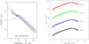 |
Fig. A.2. Luminosity in L⊙ vs time in years of SSPs (left panel) with the Salpeter IMF (in number of stars per mass interval) with exponent -2.5 and total SSP mass of 5.826 M⊙. The chemical compositions of the SSPs and associated color code are the same as in Fig. A.1. Model galaxies with infall calculated by the authors (right panel). The color code indicates the total baryonic mass of the galaxy in M⊙ whose value is also displayed in the label of each curve. The timescale of gas infall is τ = 1 Gyr. The peak in luminosity corresponds to the maximum SFR. The galaxy models are described by D’Onofrio & Chiosi (2023). |
(b) The case of two objects with different mass but the same age (old). Suppose M1 = 1012 M⊙, L1 = 1011 L⊙, and M2 = 1011 M⊙, L2 = 1010 L⊙. The total mass is M = 1.1 × 10¹² M⊙ and the total luminosity is L = 1.1 × 10¹¹ L⊙. Therefore, α1 = 0.909, h1 = 0.909 and α2 = 0.091, h2 = 0.091. The total luminosity is L = (0.909 + 0.091)L, that is, the light is dominated by the most massive galaxy. The merger has increased the total luminosity by about 10%. This is a sort of lower limit because a dry merger between two galaxies of the same age and differing in mass by more than a factor of ten would, under normal circumstances, be undetectable.
(c) In the case of two galaxies with different mass and different age, and therefore different luminosity, the total luminosity may show the effect of the younger object. Consider the following galaxies, of M1 = 1012 M⊙, L1 = 1011 L⊙ (the old object), and M2 = 1011 M⊙, L2 = 5 × 10¹⁰ L⊙ (the young object, taken near the peak value). After merging, the total mass is M = 1.1 × 10¹² M⊙ while the total luminosity is L ≃ 1.5 × 10¹¹ L⊙. Therefore, α1 = 0.909, h1 = 0.667, and α2 = 0.091, h2 = 0.333. The contribution from the less massive but younger object is important, about half that produced by the more massive but older object. Other combinations of masses and ages, and therefore luminosities, can be easily derived from eq.(A.5). Effects due to differences in the mean chemical composition of the stellar contents can be ignored at a first-order approximation.
Wet mergers (with additional star formation). In this case, in eq.(A.5), M3 ≠ 0 and L3 ≠ 0. The major difference with respect to the previous cases is that the stellar activity induced by the merger can be approximated by a single giant SSP with its own mass and luminosity. The total light emitted by M3 is L3 = (LSSP/MSSP)×M3. Now the interval spanned by the luminosity at aging SSP is much wider than before, and so the effects can be large, depending on the age. For the merging galaxies, we assume M1 = 1012 M⊙, L1 = 1011 L⊙, and M2 = 1011 M⊙, L2 = 1010 L⊙. Finally, for the mass of the giant SSP simulating the induced star formation event, we adopt M3 = 1010 M⊙. The total mass is M = 1.11 × 10¹² M⊙. For the associated luminosity, we adopt three values corresponding to a very young, high-luminosity SSP with L3 = 1 × 10¹¹ L⊙; an intermediate age, lower luminosity SSP with L3 = 1 × 10¹⁰ L⊙; and an old age, low luminosity SSP with L3 = 1 × 10⁹ L⊙. In the first case, the total luminosity is L = 2.1 × 10¹¹ L⊙, whose relative components are h1 = 0.476, h2 = 0.048, and h3 = 0.476. The burst of star formation contributes to half of the total light and 1% of the total mass. This is a rapidly transient situation that fades on a short timescale. In the second case, the total light is L = 1.2 × 10¹⁰ L⊙, and the relative contributions to the luminosity are h1 = 0.834, h2 = 0.083, h3 = 0.083; the burst of star formation contributes to about 10% of the light, that is equal to the contribution of the less massive old galaxy. In the last case, the SSP is very old; the three relative contributions are h1 = 0.908, h2 = 0.091, and h3 = 0.009. The occurrence of the burst is nearly undetectable. Other combinations of the parameters can be tested with similar results.
What we learn from these simple tests is that in the case of dry mergers, but for the merger between objects of similar mass in which the mass and light are increased by a factor of two, the effect of mergers among objects with different masses and ages barely affect the light of the originally dominant object. Wet mergers with induced star formation more efficiently leave their fingerprints on the light of the post-merger galaxy. Unfortunately, the bright phase is of short duration —the timescale required by the SSP to evolve from a turnoff in the range of bright massive stars (say 20 M⊙ with a lifetime of a few Myr) down to a turnoff in the range of low-mass stars (say below 2 M⊙ with a lifetime of about 1 Gyr); see the panel of Fig. A.1. Therefore, it is by far more probable to catch a galaxy that has undergone a wet merger when the burst of star formation has already faded down to low luminosities. This is an interesting result that could explain why the Faber-Jackson relation and the fundamental plane we see today show little scatter in the observational distribution of galaxies.
All Tables
Slopes of the Ie − Re, Re − σ, Ie − σ, and Re − M* planes for different values of β.
All Figures
|
Fig. 1. Comparison between the data of Illustris-1 and Illustris-TNG100. The black lines mark the TNG data, while the red ones the Illustris-1 data. The solid line refers to the data at z = 0, while the dashed lines to the data at z = 4. From top left to bottom right we show: the effective radius Re (enclosing half the total luminosity or half the total stellar mass (for TNG); the effective surface brightness Ie; the central star velocity dispersion σ; the stellar mass-to-light ratio (M*/L); the total luminosity (in solar units); and the total stellar mass (in solar units). |
| In the text | |
|
Fig. 2. The Re − M* (left panel) and the Ie − Re (right panel) planes for the WINGS galaxy sample. LTGs (black dots) and ETGs (open circles) share the same distributions in these SSRs. The effective radius Re is given in kiloparsecs in the Re − M* plane and in parsecs in the Ie − Re plane. Masses are given in solar units. |
| In the text | |
|
Fig. 3. The Re − M* plane and the three different projections of the FP. The black dots are the WINGS observational data. The red and blue dots are the data extracted from Illustris-1 and Illustris TNG-100, respectively. The galaxies with log(Re) < 2.5 are not plotted here in order to better show the bulk of the galaxy distribution. |
| In the text | |
|
Fig. 4. Fundamental plane at redshift z = 1. The black filled circles are the data of di Serego Alighieri et al. (2005). The red and blue circles are the data from Illutris-1 and IllustrisTNG, respectively. The FP was determined considering only the galaxies with masses in the same range as those of the observational sample (those with M* > 1010 M⊙). |
| In the text | |
|
Fig. 5. The Ie − Re plane at different redshift for Illutris-1. From top left to bottom right, we can see the distribution of galaxies at z = 4, z = 3, z = 2.2, z = 1.6, z = 1.0, z = 0.6, z = 0.2, and z = 0. The colored dots mark the galaxies with β > 0 at each epoch, whereas the black symbols mark those with β ≤ 0. The crosses mark the galaxies with SFR greater than the mean ⟨SFR⟩ at each epoch, while the open squares show those with SFR lower than ⟨SFR⟩. The arrows indicate the average direction of motion predicted on the basis of the values of β from Eq. (3); see also Table 1. The colored arrows mark the average for the galaxies with β > 0 and the black arrows those with β ≤ 0. Their length is not related or proportional to any other quantity; it was chosen for graphical reasons. |
| In the text | |
|
Fig. 6. The Ie − Re plane at different redshift for the TNG-100 data. From top left to bottom right, we show the distribution of galaxies at z = 4, z = 3, z = 2.2, z = 1.0, and z = 0. The colored dots mark the galaxies with β > 0 at each epoch, whereas the black symbols mark those with β ≤ 0. The crosses mark the galaxies with SFR greater than the mean ⟨SFR⟩ at each epoch, while the open squares show those with SFR lower than ⟨SFR⟩. The arrows indicate the average direction of motion predicted on the basis of the values of β from Eq. (3); see also Table 1. The colored arrows mark the average for the galaxies with β > 0 and the black arrows show those with β ≤ 0. Their length is not related or proportional to any other quantity; it was chosen for graphical reasons. |
| In the text | |
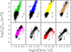 |
Fig. 7. The Ie − σ plane for the Illustris-1 data. Symbols and colors are as in Fig. 5. |
| In the text | |
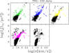 |
Fig. 8. The Ie − σ plane for the IllustrisTNG data. Symbols and colors are as in Fig. 6. |
| In the text | |
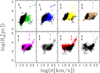 |
Fig. 9. The Re − σ plane for Illutris-1. Symbols and colors are as in Fig. 6. |
| In the text | |
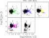 |
Fig. 10. The Re − σ plane for IllustrisTNG. Symbols and colors are as in Fig. 7. |
| In the text | |
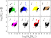 |
Fig. 11. The Re − M* plane for Illustris-1. Symbols and colors as in Fig. 5. |
| In the text | |
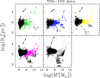 |
Fig. 12. The Re − M* plane for IllustrisTNG. Symbols and colors are as in Fig. 6. |
| In the text | |
|
Fig. 13. The β − log(Ie) plane. The colored dots follow the same color code as in Fig. 5, marking the galaxies at different redshift epochs. The black dots are the data of the WINGS database at z = 0. |
| In the text | |
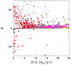 |
Fig. 14. The β − SFR plane. The colored dots and symbols as in Fig. 13. |
| In the text | |
|
Fig. 15. The β − log(Ms) (stellar mass) plane. The color code and symbols are the same as in previous figures. |
| In the text | |
|
Fig. 16. The β − [log(2T)−log(Ω)] plane. The color code and symbols are the same as in previous figures. |
| In the text | |
|
Fig. 17. Histogram of β for model galaxies of the Illustris-1 (red line) and IllustrisTNG (blue line) samples as a function of redshift. |
| In the text | |
|
Fig. 18. The SSRs for eight single galaxies. The different colors mark the single galaxies. The positions in the diagram connected by the colored lines mark the distribution at different redshift epochs. |
| In the text | |
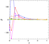 |
Fig. 19. The β − z plane for eight single galaxies. Colors are as in Fig. 18. |
| In the text | |
|
Fig. A.1. Stellar mass in M⊙ vs age in years (left panel). The asterisks along each curve are the star masses in the mass interval 0.6 to 120 M⊙. The color code of each curve indicates the chemical composition. Curves are also labeled in accordance with the mass abundance of metals Z according to the law ΔY/ΔZ = 2.5, where Y is the mass abundance of helium and the initial values are Z0 = 0.0001 and Y0 = 0.23. The values of the metalliciies are Z = 0.0001 (black), Z = 0.0004 (blue), Z = 0.004 (green), Z = 0.008 (magenta), Z = 0.020 (red), and Z = 0.050 (dark red). The mass abundance of hydrogen is given by X = 1 − Y − Z. Same as in the left panel but for luminosity vs age (right panel). The luminosity dips at ages above 1 to 1.5 Gyr correspond to the transition masses MHeF. Along each curve, stars more massive than MHeF undergo a quite He-ignition of the core, while those equal or lighter than MHeF undergo core He-flash. |
| In the text | |
|
Fig. A.2. Luminosity in L⊙ vs time in years of SSPs (left panel) with the Salpeter IMF (in number of stars per mass interval) with exponent -2.5 and total SSP mass of 5.826 M⊙. The chemical compositions of the SSPs and associated color code are the same as in Fig. A.1. Model galaxies with infall calculated by the authors (right panel). The color code indicates the total baryonic mass of the galaxy in M⊙ whose value is also displayed in the label of each curve. The timescale of gas infall is τ = 1 Gyr. The peak in luminosity corresponds to the maximum SFR. The galaxy models are described by D’Onofrio & Chiosi (2023). |
| In the text | |
Current usage metrics show cumulative count of Article Views (full-text article views including HTML views, PDF and ePub downloads, according to the available data) and Abstracts Views on Vision4Press platform.
Data correspond to usage on the plateform after 2015. The current usage metrics is available 48-96 hours after online publication and is updated daily on week days.
Initial download of the metrics may take a while.