| Issue |
A&A
Volume 678, October 2023
|
|
|---|---|---|
| Article Number | A157 | |
| Number of page(s) | 23 | |
| Section | Numerical methods and codes | |
| DOI | https://doi.org/10.1051/0004-6361/202346488 | |
| Published online | 23 October 2023 | |
Gammapy: A Python package for gamma-ray astronomy
1
Center for Astrophysics | Harvard and Smithsonian,
USA
e-mail: This email address is being protected from spambots. You need JavaScript enabled to view it.
2
Université de Paris Cité, CNRS, Astroparticule et Cosmologie,
75013
Paris, France
3
Max-Planck-Institut für Kernphysik,
PO Box 103980,
69029
Heidelberg, Germany
4
IPARCOS Institute and EMFTEL Department, Universidad Complutense de Madrid,
28040
Madrid, Spain
5
Institut de Física d’Altes Energies (IFAE), The Barcelona Institute of Science and Technology,
Campus UAB, Bellaterra,
08193
Barcelona, Spain
6
INAF/IASF Palermo,
Via U. La Malfa, 153,
90146
Palermo PA, Italy
7
Instituto de Astrofísica de Andalucia-CSIC,
Glorieta de la Astronomia s/n,
18008
Granada, Spain
8
Point 8 GmbH
Rheinlanddamm 201,
44139
Dortmund, Germany
9
Astroparticle Physics, Department of Physics, TU Dortmund University,
Otto-Hahn-Str. 4a,
44227
Dortmund, Germany
10
Université Paris-Saclay, Université Paris Cité, CEA, CNRS, AIM,
91191
Gif-sur-Yvette, France
11
Departament de Física Quàntica i Astrofísica (FQA), Universitat de Barcelona (UB),
c. Martí i Franqués, 1,
08028
Barcelona, Spain
12
Institut de Ciències del Cosmos (ICCUB), Universitat de Barcelona (UB),
c. Martí i Franqués, 1,
08028
Barcelona, Spain
13
Institut d’Estudis Espacials de Catalunya (IEEC),
c. Gran Capità, 2-4,
08034
Barcelona, Spain
14
Departament de Física Quàntica i Astrofísica, Institut de Ciències del Cosmos, Universitat de Barcelona, IEEC-UB,
Martí i Franquès, 1,
08028
Barcelona, Spain
15
Deutsches Elektronen-Synchrotron (DESY),
15738
Zeuthen, Germany
16
Institute of physics, Humboldt-University of Berlin,
12489
Berlin, Germany
17
Université Savoie Mont-Blanc, CNRS, Laboratoire d’Annecy de Physique des Particules - IN2P3,
74000
Annecy, France
18
Max Planck Institute for extraterrestrial Physics,
Giessenbachstrasse,
85748
Garching, Germany
19
Laboratoire Univers et Théories, Observatoire de Paris, Université PSL, Université Paris Cité, CNRS,
92190
Meudon, France
20
Max Planck Computing and Data Facility,
Gießenbachstraße 2,
85748
Garching, Germany
21
School of Physics, University of the Witwatersrand,
1 Jan Smuts Avenue, Braamfontein,
Johannesburg
2050, South Africa
22
The Hong Kong University of Science and Technology, Department of Electronic and Computer Engineering,
PR China
23
Cherenkov Telescope Array Observatory gGmbH (CTAO gGmbH)
Saupfercheckweg 1,
69117
Heidelberg, Germany
24
Erlangen Centre for Astroparticle Physics (ECAP), Friedrich-Alexander-Universität Erlangen-Nürnberg,
Nikolaus-Fiebiger Strasse 2,
91058
Erlangen, Germany
25
IRFU, CEA, Université Paris-Saclay,
91191
Gif-sur-Yvette, France
26
Stocadro GmbH
Arthur-Hoffmann-Straße 95,
04275
Leipzig, Germany
27
Meteo France International,
31100
Toulouse, France
28
Université Bordeaux, CNRS, LP2I Bordeaux, UMR
5797
France
29
Sorbonne Université, Université Paris Diderot, Sorbonne Paris Cité, CNRS/IN2P3, Laboratoire de Physique Nucléaire et de Hautes Energies, LPNHE,
4 Place Jussieu,
75252
Paris, France
30
Academic Computer Centre Cyfronet, AGH University of Science and Technology,
Krakow, Poland
31
Caltech/IPAC,
MC 100-22,
1200 E. California Boulevard,
Pasadena, CA
91125, USA
32
Institut für Astro- und Teilchenphysik, Leopold-Franzens-Universität Innsbruck,
6020
Innsbruck, Austria
Received:
23
March
2023
Accepted:
7
July
2023
Abstract
Context. Traditionally, TeV-γ-ray astronomy has been conducted by experiments employing proprietary data and analysis software. However, the next generation of γ-ray instruments, such as the Cherenkov Telescope Array Observatory (CTAO), will be operated as open observatories. Alongside the data, they will also make the associated software tools available to a wider community. This necessity prompted the development of open, high-level, astronomical software customized for high-energy astrophysics.
Aims. In this article, we present Gammapy, an open-source Python package for the analysis of astronomical γ-ray data, and illustrate the functionalities of its first long-term-support release, version 1.0. Built on the modern Python scientific ecosystem, Gammapy provides a uniform platform for reducing and modeling data from different γ-ray instruments for many analysis scenarios. Gammapy complies with several well-established data conventions in high-energy astrophysics, providing serialized data products that are interoperable with other software packages.
Methods. Starting from event lists and instrument response functions, Gammapy provides functionalities to reduce these data by binning them in energy and sky coordinates. Several techniques for background estimation are implemented in the package to handle the residual hadronic background affecting γ-ray instruments. After the data are binned, the flux and morphology of one or more γ-ray sources can be estimated using Poisson maximum likelihood fitting and assuming a variety of spectral, temporal, and spatial models. Estimation of flux points, likelihood profiles, and light curves is also supported.
Results. After describing the structure of the package, we show, using publicly available gamma-ray data, the capabilities of Gammapy in multiple traditional and novel γ-ray analysis scenarios, such as spectral and spectro-morphological modeling and estimations of a spectral energy distribution and a light curve. Its flexibility and its power are displayed in a final multi-instrument example, where datasets from different instruments, at different stages of data reduction, are simultaneously fitted with an astrophysical flux model.
Key words: methods: statistical / astroparticle physics / methods: data analysis / gamma rays: general
© The Authors 2023
 Open Access article, published by EDP Sciences, under the terms of the Creative Commons Attribution License (https://creativecommons.org/licenses/by/4.0), which permits unrestricted use, distribution, and reproduction in any medium, provided the original work is properly cited.
This article is published in open access under the Subscribe to Open model. This email address is being protected from spambots. You need JavaScript enabled to view it. to support open access publication.
1 Introduction
Modern astronomy offers the possibility to observe and study astrophysical sources across all wavelengths. The γ-ray range of the electromagnetic spectrum provides us with insights into the most energetic processes in the Universe such as those accelerating particles in the surroundings of black holes or remnants of supernova explosions.
In general, γ-ray astronomy relies on the detection of individual photon events and reconstruction of their incident direction as well as energy. As in other branches of astronomy, this can be achieved by satellite as well as ground-based γ-ray instruments. Space-borne instruments such as the Fermi Large Area Telescope (LAT) rely on the pair-conversion effect to detect γ-rays and track the positron-electron pairs created in the detector to reconstruct the incident direction of the incoming γ-ray. The energy of the photon is estimated using a calorimeter at the bottom of the instrument. The energy range of instruments such as Fermi-LAT (Atwood et al. 2009), referred to as “high energy” (HE), goes approximately from tens of Megaelectronvolts to hundreds of Gigaelectronvolts.
Ground-based instruments, instead, use Earth’s atmosphere as a particle detector, relying on the effect that cosmic γ-rays interacting in the atmosphere create large cascades of secondary particles, so called “air showers”, that can be observed from the ground. Ground-based γ-ray astronomy relies on the observation of these extensive air showers to estimate the primary γ-ray photons’ incident direction and energy. These instruments operate in the so-called “very high energy” (VHE) regime, covering the energy range from a few tens of Gigaelectronvolts up to Petaelectronvolts. There are two main categories of ground-based instruments.
First there are imaging atmospheric Cherenkov telescopes (IACTs), which obtain images of the atmospheric showers by detecting the Cherenkov radiation emitted by charged particles in the cascade and they use these images to reconstruct the properties of the incident particle. Those instruments have a limited field of view (FoV) and duty cycle, but good energy and angular resolution.
Second there are water Cherenkov detectors (WCDs), that detect particles directly from the tail of the shower when it reaches the ground. These instruments have a very large FoV, and large duty-cycle, but a higher energy threshold and lower signal-to-noise ratios compared to IACTs (de Naurois & Mazin 2015).
While Fermi-LAT data and analysis tools have been public since the early years of the project (Atwood et al. 2009), ground-based γ-ray astronomy has been historically conducted through experiments operated by independent collaborations, each relying on their own proprietary data and analysis software developed as part of the instrument. While this model has been successful so far, it does not permit data from several instruments to be combined easily. This lack of interoperability currently limits the full exploitation of the available γ-ray data, especially in light of the fact that different instruments often have complementary sky coverages, and the various detection techniques have complementary properties in terms of the energy range covered, duty cycle, and spatial resolution.
The Cherenkov Telescope Array Observatory (CTAO) will be the first ground-based γ-ray instrument to be operated as an open observatory. Its high-level data1 will be shared publicly after some proprietary period, along with the software required to analyze them. The adoption of an open and standardized γ-ray data format, besides being a necessity for future observatories such as CTA, will be extremely beneficial to the current generation of instruments, eventually allowing their data legacies to be exploited even beyond the end of their scientific operations.
The usage of a common data format is facilitated by the remarkable similarity of the data reduction workflow of all γ-ray telescopes. After data calibration, shower events are reconstructed and a gamma-hadron separation is applied to reject cosmic-ray-initiated showers and build lists of γ-ray-like events. The latter can then be used, taking into account the observation-specific instrument response functions (IRFs), to derive scientific results, such as spectra, sky maps, or light curves. Once the data is reduced to a list of events with reconstructed physical properties of the primary particle, the information is independent of the data-reduction process, and, eventually, of the detection technique. This implies, for example, that high-level data from IACTs and WCDs can be represented with the same data model. The efforts to create a common format usable by various instruments converged in the so-called data formats for γ-ray astronomy initiative (Deil et al. 2017; Nigro et al. 2021), abbreviated to gamma-astro-data-formats (GADF). This community-driven initiative proposes prototypical specifications to produce files based on the flexible image transport system (FITS) format (Pence et al. 2010) encapsulating this high-level information. This is realized by storing a list of γ-ray-like events with their reconstructed and observed quantities such as energy, incident direction and arrival time, and a parameterization of the IRFs associated with the event list data.
In the past decade, Python has become extremely popular as a scientific programming language, in particular in the field of data sciences. This success is mostly attributed to the simple and easy to learn syntax, the ability to act as a “glue” language between different programming languages, and last but not least the rich ecosystem of packages and its open and supportive community (Momcheva & Tollerud 2015). In the sub-field of computational astronomy, the Astropy project (Astropy Collaboration 2013) was created in 2012 to build a community-developed core Python package for astronomy. It offers basic functionalities that astronomers of many fields need, such as representing and transforming astronomical coordinates, manipulating physical quantities including units, as well as reading and writing FITS files.
The Gammapy project was started following the model of Astropy, with the objective of building a common software library for γ-ray data analysis (Donath et al. 2015). The core of the idea is illustrated in Fig. 1. The various γ-ray instruments can export their data to a common format (GADF) and then combine and analyze them using a common software library. The Gammapy package is an independent community-developed software project. It has been selected to be the core library for the science analysis tools of CTA, but it also involves contributors associated with other instruments. The Gammapy package is built on the scientific Python ecosystem: it uses Numpy (Harris et al. 2020) for ND data structures, Scipy (Virtanen et al. 2020) for numerical algorithms, Astropy (Astropy Collaboration 2013) for astronomy-specific functionality, iminuit (Dembinski et al. 2020) for numerical minimization, and Matplotlib (Hunter 2007) for visualization.
With the public availability of the GADF format specifications and the Gammapy package, some experiments have started to make limited subsets of their γ-ray data publicly available for testing and validating Gammapy. For example, the H.E.S.S. Collaboration released a limited test dataset (about 50 h of observations taken between 2004 and 2008) based on the GADF format (H.E.S.S. Collaboration 2018a) for data level 3 (DL3) γ-ray data. This data release served as a basis for validation of open analysis tools, including Gammapy (see e.g., Mohrmann et al. 2019). Two observations of the Crab nebula have been released by the MAGIC Collaboration (MAGIC Collaboration 2016). Using these public data from Fermi-LAT, H.E.S.S., MAGIC, and additional observations provided by FACT and VERITAS, the authors of Nigro et al. (2019) presented a combined analysis of γ-ray data from different instruments for the first time. Later the HAWC Collaboration also released a limited test dataset of the Crab Nebula, which was used to validate the Gammapy package in Albert et al. (2022).
The increased availability of public data that followed the definition of a common data format, and the development of Gammapy as a community-driven open software, led the way toward a more open science in the VHE γ-ray astronomy domain. The adoption of Gammapy as science tools strengthens the commitment of the future CTA Observatory to the findable, accessible, interoperable, and reusable (FAIR) principles (Wilkinson et al. 2016; Barker et al. 2022) that define the key requirements for open science.
In this article, we describe the general structure of the Gammapy package, its main concepts, and organizational structure. We start in Sect. 3.3.3 with a general overview of the data analysis workflow in VHE γ-ray astronomy. Then we show how this workflow is reflected in the structure of the Gammapy package in Sect. 3, while also describing the various sub-packages it contains. Section 4 presents a number of applications, while Sect. 5 finally discusses the project organization.
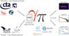 |
Fig. 1 Core idea and relation of Gammapy to different γ-ray instruments and the gamma astro data format (GADF). The top left shows the group of current and future pointing instruments based on the imaging atmospheric Cherenkov technique (IACT). This includes instruments such as the Cherenkov telescope array observatory (CTAO), the high energy stereoscopic system (H.E.S.S.), the major atmospheric gamma imaging Cherenkov telescopes (MAGIC), and the very energetic radiation imaging telescope array system (VERITAS). The lower left shows the group of all-sky instruments such as the Fermi large area telescope (Fermi-LAT) and the high altitude water Cherenkov observatory (HAWC). The calibrated data of all those instruments can be converted and stored into the common GADF data format, which Gammapy can read. The Gammapy package is a community-developed project that provides a common interface to the data and analysis of all these γ-ray instruments, allowing users to easily combine data from different instruments and perform joint analyses. Gammapy is built on the scientific Python ecosystem, and the required dependencies are shown below the Gammapy logo. |
2 Gamma-ray data analysis
The data analysis process in γ-ray astronomy is usually split into two stages. The first one deals with the data processing from detector measurement, calibration, event reconstruction and selection to yield a list of reconstructed γ-ray event candidates. This part of the data reduction sequence, sometimes referred to as low-level analysis, is usually very specific to a given observation technique and even to a given instrument.
The second stage, referred to as high-level analysis, deals with the extraction of physical quantities related to γ-ray sources and the production of high-level science products such as spectra, light curves and catalogs. The core of the analysis consists in predicting the result of an observation by modeling the flux distribution of an astrophysical object and pass it through a model of the instrument. The methods applied here are more generic and are broadly shared across the field. The similarity in the high-level analysis conceptionally also allow for easily combining data from multiple instruments. This part of the data analysis is supported by Gammapy.
2.1 DL3: events and instrument response functions
An overview of the typical steps in the high level analysis is shown in the upper row of Fig. 2. The high level analysis starts at the DL3 data level, where γ-ray data is represented as lists of γ-ray-like events and their corresponding IRFs R and ends at the DL5/6 data level, where the physically relevant quantities such as fluxes, spectra and light curves of sources have been derived. DL3 data are typically bundled into individual observations, corresponding to stable periods of data acquisition. For IACT instruments, for which the GADF data model and Gammapy were initially conceived, this duration is typically tobs = 15-30 min. Each observation is assigned a unique integer ID for reference. The event list is just a simple table with one event per row and the measured event properties as columns. These properties for example, include reconstructed incident direction and energy, arrival time and reconstruction quality.
A common assumption for the instrument response is that it can be simplified as the product of three independent functions:
 (1)
(1)
where
Aeff (ptrue, Etrue) is the effective collection area of the detector. It is the product of the detector collection area times its detection efficiency at true energy Etrue and position ptrue.
PS F(p|ptrue, Etrue) is the point spread function (PSF). It gives the probability density of measuring a direction p when the true direction is ptrue and the true energy is Etrue. γ-ray instruments typically consider radial symmetry of the PSF. With this assumption the probability density PS F (Δp|ptrue, Etrue) only depends on the angular separation between true and reconstructed direction defined by Δp = ptrue − p.
Edisp(E|ptrue, Etrue) is the energy dispersion. It gives the probability to reconstruct the photon at energy E when the true energy is Etrue and the true position ptrue. γ-ray instruments consider Edisp(μ|ptrue, Etrue), the probability density of the event migration,
 .
.
In addition to the instrument characteristics described above, there is also the instrumental background, that results from hadronic events being misclassified as γ-ray events. These events constitute a uniform background to the γ-ray events. For Fermi-LAT the residual hadronic background is very small (<1%) because of its veto layer and can often be neglected. For IACTs and WCDs in contrast, the background can account for a very large part (>95%) of the events and must be treated accordingly in the analysis. As the background is very specific to the instrument, Gammapy typically relies on the background models provided with the DL3 data. The background usually only depends on the reconstructed event position and energy Bkg(p, E). However in general all IRFs depend on the geometrical parameters of the detector, such as location of an event in the FoV or the elevation angle of the incoming direction of the event. Consequently IRFs might be parameterized as functions of detector specific coordinates as well.
The first step in γ-ray data analysis is the selection and extraction of a subset of observations based on their metadata including information such as pointing direction, observation time and observation conditions. All functionality related to representation, access and selection of DL3 data is available in the gammapy.data and gammapy.irf sub-packages.
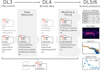 |
Fig. 2 Gammapy sub-package structure and data analysis workflow. The top row defines the different levels of data reduction, from lists of γ-ray-like events on the left (DL3), to high-level scientific products (DL5) on the right. The direction of the data flow is illustrated with the gray arrows. The gray folder icons represent the different sub-packages in Gammapy and names given as the corresponding Python code suffix, e.g., gammapy. data. Below each icon there is a list of the most important objects defined in the sub-package. The light gray folder icons show the sub-packages for the most fundamental data structures such as maps and IRFs. The bottom of the figure shows the high-level analysis sub-module with its dependency on the YAML file format. |
2.2 From DL3 to DL4: data reduction
The next step of the analysis is the data reduction, where all observation events and instrument responses are filled into or projected onto a common physical coordinate system, defined by a map geometry. The definition of the map geometry typically consists of a spectral dimension defined by a binned energy axis and of spatial dimensions, which either define a spherical projection from celestial coordinates to a pixelized image space ora single region on the sky.
After all data have been projected onto the same geometry, it is typically required to improve the residual hadronic background estimate. As residual hadronic background models can be subject to significant systematic uncertainties, these models can be improved by taking into account actual data from regions without known γ-ray sources. This includes methods such as the ring or the FoV background normalization techniques or background measurements performed for example within reflected regions (Berge et al. 2007).
Data measured at the FoV or energy boundaries of the instrument are typically associated with a systematic uncertainty in the IRF. For this reason this part of the data is often excluded from subsequent analysis by defining regions of “safe” data in the spatial as well as energy dimension. All the code related to reduce the DL3 data to binned data structures is contained in the gammapy.makers sub-package.
2.3 DL4: binned data structures
The counts data and the reduced IRFs in the form of maps are bundled into datasets that represent the fourth data level (DL4). These reduced datasets can be written to disk, in a format specific to Gammapy to allow users to read them back at any time later for modeling and fitting. Different variations of such datasets support different analysis methods and fit statistics. The datasets can be used to perform a joint-likelihood fit, allowing one to combine different measurements from different observations, but also from different instruments or event classes. They can also be used for binned simulation as well as event sampling to simulate DL3 events data.
Binned maps and datasets, which represent a collection of binned maps, are defined in the gammapy.maps and gammapy.datasets sub-packages, respectively.
2.4 From DL4 to DL5/6: modeling and fitting
The next step is then typically to model the datasets using binned Poisson maximum likelihood fitting. Assuming Poisson statistics per bin the log-likelihood of an observation is given by the Cash statistics (Cash 1979):
 (2)
(2)
where the expected number of events for the observation is given by forward folding a source model through the instrument response:
![Mathematical equation: $\matrix{ {{N_{{\rm{Pred}}}}\left( {p,E;\hat \theta } \right)\,\,{\rm{d}}p\,{\rm{d}}E = {E_{{\rm{disp}}}}\,\,\left[ {PS\,F\,\,\left( {{A_{{\rm{eff}}}} \cdot {t_{{\rm{obs}}}} \cdot {\rm{\Phi }}\left( {\hat \theta } \right)} \right)} \right].} \hfill \cr {\,\,\,\,\,\,\,\,\,\,\,\,\,\,\,\,\,\,\,\,\,\,\,\,\,\,\,\,\,\,\,\,\,\,\,\,\,\,\,\,\,\,\,\,\,\,\,\,\,\,\,\,\,\, + Bkg\left( {p,E} \right) \cdot {t_{{\rm{obs}}}}} \hfill \cr }$](/articles/aa/full_html/2023/10/aa46488-23/aa46488-23-eq4.png) (3)
(3)
The equation includes the IRF components described in the previous section, as well as an analytical model to describe the intensity of the radiation from γ-ray sources as a function of the energy, Etrue, and of the position in the FoV, ptrue:
![Mathematical equation: ${\rm{\Phi }}\left( {{p_{{\rm{true}}}},{E_{{\rm{true}}}};\hat \theta } \right),\,\left[ {\rm{\Phi }} \right] = {\rm{Te}}{{\rm{V}}^{ - 1}}\,{\rm{c}}{{\rm{m}}^{ - 2}}\,{{\rm{s}}^{ - 1}},$](/articles/aa/full_html/2023/10/aa46488-23/aa46488-23-eq5.png) (4)
(4)
where  is a set of model parameters that can be adjusted in a fit.
Observations can be either modeled individually, or in a joint likelihood analysis. In the latter case the total (joint) log-likelihood is given by the sum of the log-likelihoods per observation ℒ = Σ i = 0MC〉 for M observations. Other fit statistics such as WStat (Arnaud et al. 2023), where the background is estimated from an independent measurement or a simple χ2 for flux points are also often used and are supported by Gammapy as well. Models can be simple analytical models or more complex ones from radiation mechanisms of accelerated particle populations such as inverse Compton or π0 decay.
Independently or subsequently to the global modeling, the data can be regrouped to compute flux points, light curves and flux maps as well as significance maps in different energy bands.
Parametric models and all the functionality related to fitting is implemented in gammapy.modeling and gammapy.estimators, where the latter is used to compute higher level science products such as flux and significance maps, light curves or flux points.
3 Gammapy package
3.1 Overview
The Gammapy package is structured into multiple sub-packages. Figure 2 also shows the overview of the different sub-packages and their relation to each other. The definition of the content of the different sub-packages follows mostly the stages of the data reduction workflow described in the previous section. Subpackages either contain structures representing data at different reduction levels or algorithms to transition between these different levels. In the following sections, we will introduce all sub-packages and their functionalities in more detail. In the online documentation we also provide an overview of all the Gammapy sub-packages2.
3.2 gammapy.data
The gammapy.data sub-package implements the functionality to select, read, and represent DL3 γ-ray data in memory. It provides the main user interface to access the lowest data level. Gammapy currently only supports data that is compliant with v0.2 and v0.3 of the GADF data format.
A typical usage example is shown in Fig. 3. First a DataStore object is created from the path of the data directory. The directory contains an observation as well as a FITS HDU3 index file which assigns the correct data and IRF FITS files and HDUs to the given observation ID. The DataStore object gathers a collection of observations and provides ancillary files containing information about the telescope observation mode and the content of the data unit of each file. The DataStore allows for selecting a list of observations based on specific filters.
The DL3 level data represented by the Observation class consist of two types of elements: first, the list of γ-ray events which is represented by the EventList class. Second, a set of associated IRFs, providing the response of the system, typically factorized in independent components as described in Sect. 3.3. The separate handling of event lists and IRFs additionally allows for data from non-IACT γ-ray instruments to be read. For example, to read Fermi-LAT data, the user can read separately their event list (already compliant with the GADF specifications) and then find the appropriate IRF classes representing the response functions provided by Fermi-LAT, see example in Sect. 4.4.
3.3 gammapy.irf
The gammapy.irf sub-package contains all classes and functionalities to handle IRFs in a variety of functional forms. Usually, IRFs store instrument properties in the form of multidimensional tables, with quantities expressed in terms of energy (true orreconstructed), off-axis angles orcartesian detectorcoor-dinates. The main quantities stored in the common γ-ray IRFs are the effective area, energy dispersion, PSF and background rate. The gammapy.irf sub-package can open and access specific IRF extensions, interpolate and evaluate the quantities of interest on both energy and spatial axes, convert their format or units, plot or write them into output files. In the following, we list the main classes of the sub-package:
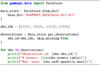 |
Fig. 3 Using gammapy.data to access DL3 level data with a DataStore object. Individual observations can be accessed by their unique integer observation id number. The actual events and instrument response functions can be accessed as attributes on the Observation object, such as .events or .aeff for the effective area information. The output of the code example is shown in Fig. A.1. |
3.3.1 Effective area
Gammapy provides the class EffectiveAreaTable2D to manage the effective area, which is usually defined in terms of true energy and offset angle. The class functionalities offer the possibility to read from files or to create it from scratch. The EffectiveAreaTable2D class can also convert, interpolate, write, and evaluate the effective area for a given energy and offset angle, or even plot the multidimensional effective area table.
3.3.2 Point spread function
Gammapy allows users to treat different kinds of PSFs, in particular, parametric multidimensional Gaussian distributions (EnergyDependentMultiGaussPSF) or King profile functions (PSFKing). The EnergyDependentMultiGaussPSF class is able to handle up to three Gaussians, defined in terms of amplitudes and sigma given for each true energy and offset angle bin. The general ParametricPSF class allows users to create a custom PSF with a parametric representation different from Gaussian(s) or King profile(s). The generic PSF3D class stores a radial symmetric profile of a PSF to represent nonparametric shapes, again depending on true energy and offset from the pointing position.
To handle the change of the PSF with the observational offset during the analysis the PSFMap class is used. It stores the radial profile of the PSF depending on the true energy and position on the sky. During the modeling step in the analysis, the PSF profile for each model component is looked up at its current position and converted into a 3D convolution kernel which is used for the prediction of counts from that model component.
3.3.3 Energy dispersion
For IACTs, the energy resolution and bias, sometimes called energy dispersion, is typically parameterized in terms of the so-called migration parameter μ. The distribution of the migration parameter is given at each offset angle and true energy. The main subclasses are the EnergyDispersion2D which is designed to handle the raw instrument description, and the EDispKernelMap, which contains an energy dispersion matrix per sky position, that is, a 4D sky map where each position is associated with an energy dispersion matrix. The energy dispersion matrix is a representation of the energy resolution as a function of the true energy only and implemented in Gammapy by the subclass EDispKernel.
3.3.4 Instrumental background
The instrumental background rate can be represented as either a 2D data structure named Background2D or a 3D one named Background3D. The background rate is stored as a differential count rate, normalized per solid angle and energy interval at different reconstructed energies and position in the FoV. In the Background2D case, the background is expected to follow a radially symmetric shape and changes only with the offset angle from FoV center. In the Background3D case, the background is allowed to vary with longitude and latitude of a tangential FoV coordinates system.
Some example IRFs read from public data files and plotted with Gammapy are shown in Fig. 4. More information on gammapy.irf can be found in the online documentation4.
3.4 gammapy.maps
The gammapy.maps sub-package provides classes that represent data structures associated with a set of coordinates or a region on a sphere. In addition it allows one to handle an arbitrary number of nonspatial data dimensions, such as time or energy. It is organized around three types of structures: geometries, sky maps and map axes, which inherit from the base classes Geom, Map and MapAxis respectively.
The geometry object defines the pixelization scheme and map boundaries. It also provides methods to transform between sky and pixel coordinates. Maps consist of a geometry instance defining the coordinate system together with a Numpy array containing the associated data. All map classes support a basic set of arithmetic and boolean operations with unit support, up and downsampling along extra axes, interpolation, resampling of extra axes, interactive visualization in notebooks and interpolation onto different geometries.
The MapAxis class provides a uniform application programming interface (API) for axes representing bins on any physical quantity, such as energy or angular offset. Map axes can have physical units attached to them, as well as define nonlinearly spaced bins. The special case of time is covered by the dedicated TimeMapAxis, which allows time bins to be noncontiguous, as it is often the case with observational times. The generic class LabelMapAxis allows the creation of axes for non-numeric entries.
To handle the spatial dimension the sub-package exposes a uniform API for the FITS World Coordinate System (WCS), the HEALPix pixelization and region-based data structure (see Fig. 5). This allows users to perform the same higher level operations on maps independent of the underlying pixelization scheme. The gammapy.maps package is also used by external packages such as “FermiPy” (Wood et al. 2017).
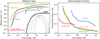 |
Fig. 4 Using gammapy.irf to read and plot instrument response functions. The left panel shows the effective area as a function of energy for the CTA, H.E.S.S., MAGIC, HAWC and Fermi-LAT instruments. The right panel shows the 68% containment radius of the PSF as a function of energy for the CTA, H.E.S.S. and Fermi-LAT instruments. The CTA IRFs are from the “prod5” production for the alpha configuration of the south and north array. The H.E.S.S. IRFs are from the DL3 DR1, using observation ID 033787. The MAGIC effective area is computed for a 20 min observation at the Crab Nebula coordinates. The Fermi-LAT IRFs use “pass8” data and are also taken at the position of the Crab Nebula. The HAWC effective area is shown for the event classes NHit = 5–9 as light gray lines along with the sum of all event classes as a black line. The HAWC IRFs are taken from the first public release of events data by the HAWC collaboration. All IRFs do not correspond to the latest performance of the instruments, but still are representative of the detector type and energy range. We exclusively relied on publicly available data provided by the collaborations. The data are also available in the gammapy-data repository. |
3.4.1 WCS maps
The FITS WCS pixelization supports a number of different projections to represent celestial spherical coordinates in a regular rectangular grid. Gammapy provides full support to data structures using this pixelization scheme. For details see Calabretta & Greisen (2002). This pixelization is typically used for smaller regions of interests, such as pointed observations and is represented by a combination of the WcsGeom and WcsNDMap class.
3.4.2 HEALPix maps
This pixelization scheme (Calabretta & Greisen 2002; Górski et al. 2005) provides a subdivision of a sphere in which each pixel covers the same surface area as every other pixel. As a consequence, however, pixel shapes are no longer rectangular, or regular. This pixelization is typically used for all-sky data, such as data from the HAWC or Fermi-LAT observatory. Gammapy natively supports the multiscale definition of the HEALPix pixelization and thus allows for easy upsampling and downsampling of the data. In addition to the all-sky map, Gammapy also supports a local HEALPix pixelization where the size of the map is constrained to a given radius. For local neighborhood operations, such as convolution, Gammapy relies on projecting the HEALPix data to a local tangential WCS grid. This data structure is represented by the HpxGeom and HpxNDMap classes.
3.4.3 Region maps
In this case, instead of a fine spatial grid dividing a rectangular sky region, the spatial dimension is reduced to a single bin with an arbitrary shape, describing a region in the sky with that same shape. Region maps are typically used together with a nonspatial dimension, for example an energy axis, to represent how a quantity varies in that dimension inside the corresponding region. To avoid the complexity of handling spherical geometry for regions, the regions are projected onto the local tangential plane using a WCS transform. This approach follows Astropy’s “Regions” package (Bradley et al. 2022), which is both used as an API to define regions for users as well as handling the underlying geometric operations. Region based maps are represented by the RegionGeom and RegionNDMap classes. More information on the gammapy.maps sub-module can be found in the online documentation5.
3.5 gammapy.datasets
The gammapy.datasets sub-package contains classes to bundle together binned data along with the associated models and likelihood function, which provides an interface to the Fit class (Sect. 3.8.2) for modeling and fitting purposes. Depending upon the type of analysis and the associated statistic, different types of Datasets are supported. The MapDataset is used for combined spectral and morphological (3D) fitting, while spectral fitting only can be performed using the SpectrumDataset. While the default fit statistics for both of these classes is the Cash (Cash 1979) statistic, there are other classes which support analyses where the background is measured from control regions, so called “off” observations. Those require the use of a different fit statistics, which takes into account the uncertainty of the background measurement. This case is covered by the MapDatasetOnOff and SpectrumDatasetOnOff classes, which use the WStat (Arnaud et al. 2023) statistic.
Fitting of precomputed flux points is enabled through FluxPointsDataset, using χ2 statistics. Multiple datasets of same or different types can be bundled together in Datasets (see e.g., Fig. 6), where the likelihood from each constituent member is added, thus facilitating joint fitting across different observations, and even different instruments across different wavelengths. Datasets also provide functionalities for manipulating reduced data, for instance stacking, sub-grouping, plotting. Users can also create their customized datasets for implementing modified likelihood methods. We also refer to our online documentation for more details on gammapy.datasets6.
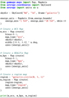 |
Fig. 5 Using gammapy.maps to create a WCS, a HEALPix and a region based data structures. The initialization parameters include consistently the positions of the center of the map, the pixel size, the extend of the map as well as the energy axis definition. The energy minimum and maximum values for the creation of the MapAxis object can be defined as strings also specifying the unit. Region definitions can be passed as strings following the DS9 region specifications http://ds9.si.edu/doc/ref/region.html. The output of the code example is shown in Fig. A.3. |
3.6 gammapy.makers
The gammapy.makers sub-package contains the various classes and functions required to process and prepare γ-ray data from the DL3 to the DL4. The end product of the data reduction process is a set of binned counts, background exposure, psf and energy dispersion maps at the DL4 level, bundled into a MapDataset object. The MapDatasetMaker and SpectrumDatasetMaker are responsible for this task for three- and 1D analyses, respectively (see Fig. 7).
The correction of background models from the data themselves is supported by specific Maker classes such as the FoVBackgroundMaker or the ReflectedRegionsBackgroundMaker. The former is used to estimate the normalization of the background model from the data themselves, while the latter is used to estimate the background from regions reflected from the pointing position.
Finally, to limit other sources of systematic uncertainties, a data validity domain is determined by the SafeMaskMaker. It can be used to limit the extent of the FoV used, or to limit the energy range to a domain where the energy reconstruction bias is below a given threshold.
More detailed information on the gammapy.makers subpackage is available online7.
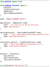 |
Fig. 6 Using gammapy.datasets to read existing reduced binned datasets. After the different datasets are read from disk they are collected into a common Datasets container. All dataset types have an associated name attribute to allow a later access by name in the code. The environment variable $GAMMAPY_DATA is automatically resolved by Gammapy. The output of the code example is shown in Fig. A.2. |
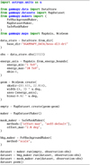 |
Fig. 7 Using gammapy.makers to reduce DL3 level data into a MapDataset. All Maker classes represent a step in the data reduction process. They take the configuration on initialization of the class. They also consistently define .run() methods, which take a dataset object and optionally an Observation object. In this way, Maker classes can be chained to define more complex data reduction pipelines. The output of the code example is shown in Fig. A.5. |
3.7 gammapy.stats
The gammapy.stats subpackage contains the fit statistics and the associated statistical estimators commonly adopted in γ-ray astronomy. In general, γ-ray observations count Poisson-distributed events at various sky positions and contain both signal and background events. To estimate the number of signal events in the observation one typically uses Poisson maximum likelihood estimation (MLE). In practice this is done by minimizing a fit statistic defined by −2 log ℒ, where ℒ is the likelihood function used. Gammapy uses the convention of a factor of 2 in front, such that a difference in log-likelihood will approach a χ2 distribution in the statistial limit.
When the expected number of background events is known, the statistic function is the so called Cash statistic (Cash 1979). It is used by datasets using background templates such as the MapDataset. When the number of background events is unknown, and an “off” measurement where only background events are expected is used, the statistic function is WStat. It is a profile log-likelihood statistic where the background counts are marginalized parameters. It is used by datasets containing “off” counts measurements such as the SpectrumDatasetOnOff, used for classical spectral analysis.
To perform simple statistical estimations on counts measurements, CountsStatistic classes encapsulate the aforementioned statistic functions to measure excess counts and estimate the associated statistical significance, errors and upper limits. They perform maximum likelihood ratio tests to estimate significance (the square root of the statistic difference) and compute likelihood profiles to measure errors and upper limits. The code example Fig. 8 shows how to compute the Li & Ma significance (Li & Ma 1983) of a set of measurements. Our online documentation provides more information on gammapy.stats8.
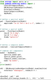 |
Fig. 8 Using gammapy.stats to compute statistical quantities such as excess, significance and asymmetric errors from counts based data. The data array such as counts, counts_off and the background efficiency ratio alpha are passed on initialization of the WStatCountsStatistic class. The derived quantities are then computed dynamically from the corresponding class attributes such as stat.n_sig for the excess and stat.sqrt_ts for the significance. The output of the code example is shown in Fig. A.4. |
3.8 gammapy.modeling
gammapy.modeling contains all the functionality related to modeling and fitting data. This includes spectral, spatial and temporal model classes, as well as the fit and parameter API.
3.8.1 Models
Source models in Gammapy (Eq. (4)) are 4D analytical models which support two spatial dimensions defined by the sky coordinates ℓ, b, an energy dimension E, and a time dimension t. To simplify the definition of the models, Gammapy uses a factorized representation of the total source model:
 (5)
(5)
The spectral component F(E), described by the SpectralModel class, always includes an amplitude parameter to adjust the total flux of the model. The spatial component G(ℓ, b, E), described by the SpatialModel class, also depends on energy, in order to consider energy-dependent sources morphology. Finally, the temporal component H(t, E), described by the TemporalModel class, also supports an energy dependency in order to consider spectral variations of the model with time.
The models follow a naming scheme which contains the category as a suffix to the class name. The spectral models include a special class of normed models, named using the NormSpectralModel suffix. These spectral models feature a dimension-less “norm” parameter instead of an amplitude parameter with physical units. They can be used as an energy-dependent multiplicative correction factor to another spectral model. They are typically used for adjusting template-based models, or, for example, to take into account the absorption effect on γ-ray spectra caused by the extra-galactic background light (EBL; EBLAbsorptionNormSpectralModel). Gammapy supports a variety of EBL absorption models, such as those from Franceschini et al. (2008); Franceschini & Rodighiero (2017), Finke et al. (2010), and Domínguez et al. (2011).
The analytical spatial models are all normalized such that they integrate to unity over the entire sky. The template spatial models may not, so in that special case they have to be combined with a NormSpectralModel.
The SkyModel class represents the factorized model in Eq. (5) (the spatial and temporal components being optional). A SkyModel object can represent the sum of several emission components: either, for example, from multiple sources and from a diffuse emission, or from several spectral components within the same source. To handle a list of multiple SkyModel objects, Gammapy implements a Models class.
The model gallery9 provides a visual overview of the available models in Gammapy. Most of the analytic models commonly used in γ-ray astronomy are built-in. We also offer a wrapper to radiative models implemented in the Naima package (Zabalza 2015). The modeling framework can be easily extended with user-defined models. For example, the radiative models of jetted Active Galactic Nuclei (AGN) implemented in Agnpy (Nigro et al. 2022), can be wrapped into Gammapy (see Sect. 3.5 of Nigro et al. 2022). An example of using gammapy.modeling.models is shown in Fig. 9. We provide more examples of user-defined models, such as a parametric model for energy dependent morphology, in the online documentation10.
3.8.2 Fit
The Fit class provides methods to optimize (“fit”), model parameters and estimate their errors and correlations. It interfaces with a Datasets object, which in turn is connected to a Models object containing the model parameters bundled into a Parameters object. Models can be unique for a given dataset, or contribute to multiple datasets, allowing one to perform ajoint fit to multiple IACT datasets, or to jointly fit IACT and Fermi-LAT datasets. Many examples are given in the tutorials.
The Fit class provides a uniform interface to multiple fitting backends:
iminuit (Dembinski et al. 2020)
scipy.optimize (Virtanen et al. 2020)
Sherpa (Refsdal et al. 2011; Freeman et al. 2001)
We note that, for now, covariance matrix and errors are computed only for the fitting with iminuit. However, depending on the problem other optimizers can perform better, so sometimes it can be useful to run a pre-fit with alternative optimization methods. In the future, we plan to extend the supported fitting backends, including for example solutions based on Markov chain Monte Carlo methods11.
 |
Fig. 9 Using gammapy.modeling.models to define a source model with a spectral, spatial and temporal component. For convenience the model parameters can be defined as strings with attached units. The spatial model takes an additional frame parameter which allow users to define the coordinate frame of the position of the model. The output of the code example is shown in Fig. A.8. |
Definition of the different SED types supported in Gammapy.
3.9 gammapy.estimators
By fitting parametric models to the data, the total γ-ray flux and its overall temporal, spectral and morphological components can be constrained. In many cases though, it is useful to make a more detailed follow-up analysis by measuring the flux in smaller spectral, temporal or spatial bins. This possibly reveals more detailed emission features, which are relevant for studying correlation with counterpart emissions.
The gammapy.estimators sub-module features methods to compute flux points, light curves, flux maps and flux profiles from data. The basic method for all these measurements is equivalent. The initial fine bins of MapDataset are grouped into larger bins. A multiplicative correction factor (the norm) is applied to the best fit reference spectral model and is fitted in the restricted data range, defined by the bin group only.
In addition to the best-fit flux norm, all estimators compute quantities corresponding to this flux. This includes: the predicted number of total, signal and background counts per flux bin; the total fit statistics of the best fit model (for signal and background); the fit statistics of the null hypothesis (background only); and the difference between both, the so-called test statistic value (TS). From this TS value, a significance of the measured signal and associated flux can be derived.
Optionally, the estimators can also compute more advanced quantities such as asymmetric flux errors, flux upper limits and 1D profiles of the fit statistic, which show how the likelihood functions varies with the flux norm parameter around the fit minimum. This information is useful in inspecting the quality of a fit, for which a parabolic shape of the profile is asymptomatically expected at the best fit values.
The base class of all algorithms is the Estimator class. The result of the flux point estimation are either stored in a FluxMaps or FluxPoints object. Both objects are based on an internal representation of the flux which is independent of the Spectral Energy Distribution (SED) type. The flux is represented by a reference spectral model and an array of normalization values given in energy, time and spatial bins, which factorizes the deviation of the flux in a given bin from the reference spectral model. This allows users to conveniently transform between different SED types. Table 1 shows an overview and definitions of the supported SED types. The actual flux values for each SED type are obtained by multiplication of the norm with the reference flux.
Both result objects support the possibility to serialize the data into multiple formats. This includes the GADF SED for-mat12, FITS-based nd sky maps and other formats compatible with Astropy’s Table and BinnedTimeSeries data structures. This allows users to further analyze the results with Astropy, for example using standard algorithms for time analysis, such as the Lomb-Scargle periodogram or the Bayesian blocks. So far, Gammapy does not support unfolding of γ-ray spectra. Methods for this will be implemented in future versions of Gammapy.
The code example shown in Fig. 10 shows how to use the TSMapEstimator objects with a given input MapDataset. In addition to the model, it allows the energy bins of the resulting flux and TS maps to be specified.
More details on the gammapy.estimators sub-module are available online13.
 |
Fig. 10 Using the TSMapEstimator object from gammapy.estimators to compute a flux, flux upper limits and TS map. The additional parameters n_sigma and n_sigma_ul define the confidence levels (in multiples of the normal distribution width) of the flux error and flux upper limit maps respectively. The output of the code example is shown in Fig. A.6. |
3.10 gammapy.analysis
The gammapy.analysis sub-module provides a high-level interface (HLI) for the most common use cases identified in γ-ray analyses. The included classes and methods can be used in Python scripts, notebooks or as commands within IPython sessions. The HLI can also be used to automatize workflows driven by parameters declared in a configuration file in YAML format. In this way, a full analysis can be executed via a single command line taking the configuration file as input.
The Analysis class has the responsibility for orchestrating the workflow defined in the configuration AnalysisConfig objects and triggering the execution of the AnalysisStep classes that define the identified common use cases. These steps include the following: observations selection with the DataStore, data reduction, excess map computation, model fitting, flux points estimation, and light curves production.
3.11 gammapy.visualization
The gammapy.visualization sub-package contains helper functions for plotting and visualizing analysis results and Gammapy data structures. This includes, for example, the visualization of reflected background regions across multiple observations, or plotting large parameter correlation matrices of Gammapy models. It also includes a helper class to split wide field Galactic survey images across multiple panels to fit a standard paper size.
The sub-package also provides matplotlib implementations of specific colormaps. Those colormaps have been historically used by larger collaborations in the VHE domain (such as MILAGRO or H.E.S.S.) as “trademark” colormaps. While we explicitly discourage the use of those colormaps for publication of new results, because they do not follow modern visualization standards, such as linear brightness gradients and accessibility for visually impaired people, we still consider the colormaps useful for reproducibility of past results.
3.12 gammapy.astro
The gammapy.astro sub-package contains utility functions for studying physical scenarios in high-energy astrophysics. The gammapy.astro.darkmatter module computes the so called J-factors and the associated γ-ray spectra expected from annihilation of dark matter in different channels, according to the recipe described in Cirelli et al. (2011).
In the gammapy.astro.source sub-module, dedicated classes exist for modeling galactic γ-ray sources according to simplified physical models, for example supernova remnant (SNR) evolution models (Taylor 1950; Truelove & McKee 1999), evolution of pulsar wind nebulae (PWNe) during the free expansion phase (Gaensler & Slane 2006), or computation of physical parameters of a pulsar using a simplified dipole spin-down model.
In the gammapy.astro.population sub-module there are dedicated tools for simulating synthetic populations based on physical models derived from observational or theoretical considerations for different classes of Galactic very high-energy γ-ray emitters: PWNe, SNRs Case & Bhattacharya (1998), pulsars Faucher-Giguère & Kaspi (2006); Lorimer et al. (2006); Yusifov & Küçük (2004) and γ-ray binaries.
While the present list of use cases is rather preliminary, this can be enriched with time by users and/or developers according to future needs.
3.13 gammapy.catalog
Comprehensive source catalogs are increasingly being provided by many high-energy astrophysics experiments. The gammapy.catalog sub-packages provides a convenient access to the most important γ-ray catalogs. Catalogs are represented by the SourceCatalog object, which contains the actual catalog as an Astropy Table object. Objects in the catalog can be accessed by row index, name of the object or any association or alias name listed in the catalog.
Sources are represented in Gammapy by the SourceCatalogObject class, which has the responsibility to translate the information contained in the catalog to Gammapy objects. This includes the spatial and spectral models of the source, flux points and light curves (if available) for each individual object. Figure 11 show how to load a given catalog and access these information for a selected source. The required catalogs are supplied in the GAMMAPY_DATA repository, such that user do not have to download them separately. The overview of currently supported catalogs, the corresponding Gammapy classes and references are shown in Table 2. Newly released relevant catalogs will be added in future.
 |
Fig. 11 Using gammapy.catalogs to access the underlying model, flux points and light-curve from the Fermi-LAT 4FGL catalog for the blazar PKS 2155-304. The output of the code example is shown in Fig. A.7. |
4 Applications
Gammapy is currently used for a variety of analyses by different IACT experiments and has already been employed in about 65 scientific publications as of 21/03/202314. In this section, we illustrate the capabilities of Gammapy by performing some standard analysis cases commonly considered in γ-ray astronomy. Beside reproducing standard methodologies, we illustrate the unique data combination capabilities of Gammapy by presenting a multi-instrument analysis, which is not possible within any of the current instrument private software frameworks. The examples shown are based on the data accessible in the gammapy-data repository, and limited by the availability of public data. We remark that, as long as the data are compliant with the GADF specifications (or its future evolutions), and hence with Gammapy’s data structures, there is no limitation on performing analyses of data from a given instrument.
4.1 1D analysis
One of the most common analysis cases in γ-ray astronomy is measuring the spectrum of a source in a given region defined on the sky, in conventional astronomy also called aperture photometry. The spectrum is typically measured in two steps: first a parametric spectral model is fitted to the data and secondly flux points are computed in a predefined set of energy bins. The result of such an analysis performed on three simulated CTA observations is shown in Fig. 12. In this case the spectrum was measured in a circular aperture centered on the Galactic Center, in γ-ray astronomy often called “on region”. For such analysis the user first chooses a region of interest and energy binning, both defined by a RegionGeom. In a second step, the events and the IRFs are binned into maps of this geometry, by the SpectrumDatasetMaker. All the data and reduced IRFs are bundled into a SpectrumDataset. To estimate the expected background in the “on region” a “reflected regions” background method was used (Berge et al. 2007), represented in Gammapy by the ReflectedRegionsBackgroundMaker class. The resulting reflected regions are illustrated for all three observations overlaid on the counts map in Fig. 12. After reduction, the data were modeled using a forward-folding method and assuming a point source with a power law spectral shape. The model was defined, using the SkyModel class with a PowerLawSpectralModel spectral component only. This model was then combined with the SpectrumDataset, which contains the reduced data and fitted using the Fit class. Based on this best-fit model, the final flux points and corresponding log-likelihood profiles were computed using the FluxPointsEstimator. The example takes <10 s to run on a standard laptop with M1 arm64 CPU.
Overview of supported catalogs in gammapy.catalog.
 |
Fig. 12 Example of a 1D spectral analysis of the Galactic Center for three simulated observations from the first CTA data challenge. The left image shows the maps of counts with the signal region in white and the reflected background regions for the three different observations overlaid in different colors. The right image shows the resulting spectral flux points and their corresponding log-likelihood profiles. The flux points are shown in orange, with the horizontal bar illustrating the width of the energy bin and the vertical bar the 1σ error. The log-likelihood profiles for each enetgy bin are shown in the background. The colormap illustrates the difference of the log-likelihood to the log-likelihood of the best fit value. |
4.2 3D analysis
The 1D analysis approach is a powerful tool to measure the spectrum of an isolated source. However, more complicated situations require a more careful treatment. In a FoV containing several overlapping sources, the ID approach cannot disentangle the contribution of each source to the total flux in the selected region. Sources with extended or complex morphology can result in the measured flux being underestimated, and heavily dependent on the choice of extraction region.
For such situations, a more complex approach is needed, the so-called 3D analysis. The three relevant dimensions are the two spatial angular coordinates and an energy axis. In this framework, a combined spatial and spectral model (that is, a SkyModel, see Sect. 3.8) is fitted to the sky maps that were previously derived from the data reduction step and bundled into a MapDataset (see Sects. 3.6 and 3.5).
A thorough description of the 3D analysis approach and multiple examples that use Gammapy can be found in Mohrmann et al. (2019). Here we present a short example to highlight some of its advantages.
Starting from the IRFs corresponding to the same three simulated CTA observations used in Sect. 4.1, we can create a MapDataset via the MapDatasetMaker. However, we will not use the simulated event lists provided by CTA but instead, use the method MapDataset.fake() to simulate measured counts from the combination of several SkyModel instances. In this way, a DL4 dataset can directly be simulated. In particular we simulate:
a point source located at (l = 0°, b = 0°) with a power law spectral shape,
an extended source with Gaussian morphology located at (l = 0.4°, b = 0.15°) with σ = 0.2° and a log parabola spectral shape,
a large shell-like structure centered on (l = 0.06°, b = 0.6°) with a radius and width of 0.6° and 0.3° respectively and a power law spectral shape.
The position and sizes of the sources have been selected so that their contributions overlap. This can be clearly seen in the significance map shown in the left panel of Fig. 13. This map was produced with the ExcessMapEstimator (see Sect. 3.9) with a correlation radius of 0.1°.
We can now fit the same model shapes to the simulated data and retrieve the best-fit parameters. To check the model agreement, we compute the residual significance map after removing the contribution from each model. This is done again via the ExcessMapEstimator. As can be seen in the middle panel of Fig. 13, there are no regions above or below 5σ, meaning that the models describe the data sufficiently well.
As the example above shows, the 3D analysis allows the morphology of the emission to be characterized and fit it together with the spectral properties of the source. Among the advantages that this provides is the ability to disentangle the contribution from overlapping sources to the same spatial region. To highlight this, we define a circular RegionGeom of radius 0.5° centered around the position of the point source, which is drawn in the left panel of Fig. 13. We can now compare the measured excess counts integrated in that region to the expected relative contribution from each of the three source models. The result can be seen in the right panel of Fig. 13. We note that all the models fitted also have a spectral component, from which flux points can be derived in a similar way as described in Sect. 4.1. The whole example takes <2 min to run on a standard laptop with M1 arm64 CPU.
 |
Fig. 13 Example of a 3D analysis for simulated sources with point-like, Gaussian and shell-like morphologies. The simulation uses “prod5” IRFs from CTA (Cherenkov Telescope Array Observatory & Cherenkov Telescope Array Consortium 2021). The left image shows a significance map (using the Cash statistics) where the three simulated sources can be seen. The middle figure shows another significance map, but this time after subtracting the best-fit model for each of the sources, which are displayed in black. The right figure shows the contribution of each source model to the circular region of radius 0.5° drawn in the left image, together with the excess counts inside that region. |
4.3 Temporal analysis
A common use case in many astrophysical scenarios is to study the temporal variability of a source. The most basic way to do this is to construct a “light curve”, which corresponds to measuring the flux of a source in a set of given time bins. In Gammapy, this is done by using the LightCurveEstimator that fits the normalization of a source in each time (and optionally energy) band per observation, keeping constant other parameters. For custom time binning, an observation needs to be split into finer time bins using the Observation. select_time method. Figure 14 shows the light curve of the blazar PKS 2155-304 in different energy bands as observed by the H.E.S.S. telescope during an exceptional flare on the night of July 29–30, 2006 (Aharonian et al. 2009). The data are publicly available as a part of the HESS-DL3-DR1 (H.E.S.S. Collaboration 2018a).
Each observation is first split into 10 min smaller observations, and spectra extracted for each of these within a 0.11° radius around the source. A PowerLawSpectralModel is fit to all the datasets, leading to a reconstructed index of 3.54 ± 0.02. With this adjusted spectral model the LightCurveEstimator runs directly for two energy bands, 0.5-1.5 TeV and 1.5–20 TeV respectively. The obtained flux points can be analytically modeled using the available or user-implemented temporal models. Alternatively, instead of extracting a light curve, it is also possible to directly fit temporal models to the reduced datasets. By associating an appropriate SkyModel, consisting of both temporal and spectral components, or using custom temporal models with spectroscopic variability, to each dataset, a joint fit across the datasets will directly return the best fit temporal and spectral parameters. The light curve data reduction and computation of flux points takes about 0.5 min to run on a standard laptop with M1 arm64 CPU.
4.4 Multi-instrument analysis
In this multi-instrument analysis example we showcase the capabilities of Gammapy to perform a simultaneous likelihood fit incorporating data from different instruments and at different levels of reduction. We estimate the spectrum of the Crab Nebula combining data from the Fermi-LAT, MAGIC and HAWC instruments.
The Fermi-LAT data are introduced at the data level DL4, and directly bundled in a MapDataset. They have been prepared using the standard “fermitools” (Fermi Science Support Development Team 2019) and selecting a region of 5° × 4° around the position of the Crab Nebula, applying the same selection criteria of the 3FHL catalog (7 yr of data with energy from 10 GeV to 2 TeV, Ajello et al. 2017).
The MAGIC data are included from the data level DL3. They consist of two observations of 20 min each, chosen from the dataset used to estimate the performance of the upgraded stereo system (MAGIC Collaboration 2016) and already included in Nigro et al. (2019). The observations were taken at small zenith angles (<30°) in wobble mode (Fomin et al. 1994), with the source sitting at an offset of 0.4° from the FoV center. Their energy range spans 80 GeV-20 TeV. The data reduction for the ID analysis is applied, and the data are reduced to a SpectrumDataset before being fitted.
HAWC data are directly provided as flux points (DL5 data level) and are read via Gammapy’s FluxPoints class. They were estimated in HAWC Collaboration (2019) with 2.5 yr of data and span an energy range 300 GeV-300 TeV.
Combining the datasets in a Datasets list, Gammapy automatically generates a likelihood including three different types of terms, two Poissonian likelihoods for Fermi-LAT’s MapDataset and MAGIC’s SpectrumDataset, and χ2 accounting for the HAWC flux points. For Fermi-LAT, a 3D forward folding of the sky model with the IRF is performed, in order to compute the predicted counts in each sky-coordinate and energy bin. For MAGIC, a ID forward-folding of the spectral model with the IRFs is performed to predict the counts in each estimated energy bin. A log parabola is fitted over almost five decades in energy 10GeV–300TeV, taking into account all flux points from all three datasets.
The result of the joint fit is displayed in Fig. 15. We remark that the objective of this exercise is illustrative. We display the flexibility of Gammapy in simultaneously fitting multi-instrument data even at different levels of reduction, without aiming to provide a new measurement of the Crab Nebula spectrum. The spectral fit takes < 10 s to run on a standard laptop with M1 arm 64 CPU.
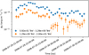 |
Fig. 14 Binned PKS 2155-304 light curve in two different energy bands as observed by the H.E.S.S. telescopes in 2006. The colored markers show the flux points in the different energy bands: the range from (0.5 TeV to 1.5 TeV is shown in blue, while the range from 1.5 TeV to 20 TeV) is shown in orange. The horizontal error illustrates the width of the time bin of 10 min. The vertical error bars show the associated asymmetrical flux errors. The marker is set to the center of the time bin. |
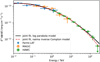 |
Fig. 15 Multi-instrument spectral energy distribution (SED) and combined model fit of the Crab Nebula. The colored markers show the flux points computed from the data of the different listed instruments. The horizontal error bar illustrates the width of the chosen energy band (EMin, EMax). The marker is set to the log-center energy of the band, that is defined by |

4.5 Broadband SED modeling
By combining Gammapy with astrophysical modeling codes, users can also fit astrophysical spectral models to γ-ray data. There are several Python packages that are able to model the γ-ray emission, given a physical scenario. Among those packages are Agnpy (Nigro et al. 2022), Naima (Zabalza 2015), Jetset (Tramacere 2020) and Gamera (Hahn et al. 2022). Typically those emission models predict broadband emission from radio, up to very high-energy γ-rays. By relying on the multiple dataset types in Gammapy those data can be combined to constrain such a broadband emission model. Gammapy provides a built-in NaimaSpectralModel that allows users to wrap a given astrophysical emission model from the Naima package and fit it directly to γ-ray data.
As an example application, we use the same multi-instrument dataset of the Crab Nebula, described in the previous section, and we apply an inverse Compton model computed with Naima and wrapped in the Gammapy models through the NaimaSpectralModel class. We describe the gamma-ray emission with an inverse Compton scenario, considering a log-parabolic electron distribution that scatters photons from:
the synchrotron radiation produced by the very same electrons
near and far infrared photon fields
and the cosmic microwave background (CMB).
We adopt the prescription on the target photon fields provided in the documentation of the “Naima” package15. The best-fit inverse Compton spectrum is represented with a red dashed line in Fig. 15. The fit of the astrophysical model takes <5 min to run on a standard laptop with M1 arm64 CPU.
More examples for modeling the broadband emission of γ-ray sources, which partly involve Gammapy are available in the online documentation of the Agnpy, Naima, Jetset and Gamera packages16,17,18,19.
4.6 Surveys, catalogs, and population studies
As a last application example we describe the use of Gammapy for large scale analyses such as γ-ray surveys, catalogs and population studies. Early versions of Gammapy were developed in parallel to the preparation of the H.E.S.S. Galactic plane survey catalog (HGPS, H.E.S.S. Collaboration 2018b) and the associated PWN and SNR populations studies (H.E.S.S. Collaboration 2018c,d).
The increase in sensitivity and angular resolution provided by the new generation of instruments scales up the number of detectable sources and the complexity of models needed to represent them accurately. As an example, if we compare the results of the HGPS to the expectations from the CTA Galactic Plane survey simulations, we jump from 78 sources detected by H.E.S.S. to about 500 detectable by CTA (Remy et al. 2021). This large increase in the amount of data to analyze and increase in complexity of modeling scenarios, requires the high-level analysis software to be both scalabale as well as performant.
In short, the production of catalogs from γ-ray surveys can be divided in four main steps: (a) data reduction, (b) object detection, (c) model fitting and model selection and (d) associations and classification. All steps can either be done directly with Gammapy or by relying on the seamless integration of Gammapy with the scientific Python ecosystem. This allows one to rely on third party functionality wherever needed. A simplified catalog analysis based on Gammapy typically includes:
The IACTs data reduction step is done in the same way described in the previous sections but scaled up to a few thousand observations. This step can be trivially parallelized by deploying the Gammapy package on a cluster.
The object detection step typically consists in finding local maxima in the significance or TS maps, computed by the ExcessMapEstimator or TSMapEstimator respectively. For this Gammapy provides a simple find_peaks method. Formore advanced methods users can rely on third party packages such as “Scikit-image” (van der Walt et al. 2014). This packages provide for example general “blob detection” algorithms and image segmentation methods such as hysteresis thresholding or the watershed transform.
During the modeling step each object is alternatively fitted with different models in order to determine their optimal parameters, and the best-candidate model. The subpackage gammapy.modeling.models offers a large variety of choices for spatial and spectral models as well as the possibility to add custom models. For the model selection Gammapy provides statisticl helper methods to perform likelihood ratio tests. But users can also rely on third party packages such as “Scikitlearn” (Pedregosa et al. 2011) to compute quantities such as the Akaike information criterion (AIC) or the Bayesian information criterion (BIC), which also allow for model selection.
For the association and classification step, which is tightly connected to population studies, we can easily compare the fitted models to the set of existing γ-ray catalogs available in gammapy.catalog. Further multi-wavelength cross-matches are usually required to characterize the sources. This can easily be achieved by relying on coordinate handling from Astropy in combination with affiliated packages such as “Astroquery” (Ginsburg et al. 2019). For more advanced source classification methods users can again rely for example on Scikit-learn to perform supervised or unsupervised clustering.
Gammapy has been successfully used for catalog studies performed on simulations of the future CTA Galactic Plane Survey (Remy et al. 2021). Besides the scientific insights they also gave us the opportunity to test the Gammapy software on complex use cases. This resulted in a number of improvements to the Gammapy package, such as as improved performance, optimized analysis strategies documented to users, and identifying the needs for future developments, including solutions for distributed computing. The catalog studies of the CTA Galactic Plane Survey simulations also allowed for detailed cross-comparison of the results obtained with the independent γ-ray analysis package “ctools” (Knödlseder et al. 2016), with very consistent results.
5 The Gammapy project
In this section, we provide an overview of the organization of the Gammapy project. We briefly describe the main roles and responsibilities within the team, as well as the technical infrastructure designed to facilitate the development and maintenance of Gammapy as a high-quality software. We use common tools and services for software development of Python open-source projects, code review, testing, package distribution and user support, with a customized solution for a versioned and thoroughly tested documentation in the form of user-friendly playable tutorials. This section concludes with an outlook on the road map for future directions.
5.1 Organizational structure
Gammapy is an international open-source project with a broad developer base and contributions and commitments from multiple groups and leading institutes in the very high-energy astrophysics domain20. The main development road maps are discussed and validated by a “Coordination Committee”, composed of representatives of the main contributing institutions and observatories. This committee is chaired by a “Project Manager” and his deputy while two “Lead Developers” manage the development strategy and organize technical activities. This institutionally driven organization, the permanent staff and commitment of supporting institutes ensure the continuity of the executive teams. A core team of developers from the contributing institutions is in charge of the regular development, which benefits from regular contributions of the community at large.
 |
Fig. 16 Overview of used programming languages and distribution of code across the different file categories in the Gammapy code base. The total number of lines is ≈50 000. |
5.2 Technical infrastructure
Gammapy follows an open-source and open-contribution development model based on the cloud repository service GitHub. A GitHub organization named “gammapy21” hosts different repositories related with the project. The software codebase may be found in the Gammapy repository (see Fig. 16 for code lines statistics). We make extensive use of the pull request system to discuss and review code contributions.
Several automated tasks are set as GitHub actions22, blocking the processes and alerting developers when failures occur. This is the case of the continuous integration workflow, which monitors the execution of the test coverage suite23 using datasets from the “gammapy-data” repository24. Tests scan not only the codebase, but also the code snippets present in docstrings of the scripts and in the RST documentation files, as well as in the tutorials provided in the form of Jupyter notebooks.
Other automated tasks, executing in the “gammapy-benchmarks25” repository, are responsible for numerical validation tests and benchmarks monitoring. Also, tasks related with the release process are partially automated, and every contribution to the codebase repository triggers the documentation building and publishing workflow within the “gammapy-docs” repository26 (see Sects. 5.3 and 5.4).
This small ecosystem of interconnected up-to-date repositories, automated tasks and alerts, is just a part of a bigger set of GitHub repositories, where most of them are related with the project but not necessary for the development of the software (i.e., project webpage, complementary high-energy astrophysics object catalogs, coding sprints and weekly developer calls minutes, contributions to conferences, other digital assets, etc). Finally, third-party services for code quality metrics are also set and may be found as status shields in the codebase repository.
5.3 Software distribution
Gammapy is distributed for Linux, Windows and Mac environments, and installed in the usual way for Python packages. Each stable release is uploaded to the Python package index27 and as a binary package to the “conda-forge” and “astropy” Anaconda repository28 channels. At this time, Gammapy is also available as a Debian Linux package29. We recommend installing the software using the “conda” installation process with an environment definition file that we provide, so to work within a virtual isolated environment with additional useful packages and ensure reproducibility.
Gammapy is indexed in the Astronomy Source Code Library30 and Zenodo31 digital libraries for software. The Zen-odo record is synchronized with the codebase GitHub repository so that every release triggers the update of the versioned record. In addition, Gammapy has been added to the Open-source scientific Software and Service Repository32 (Vuillaume et al. 2023) and indexed in the European Open Science Cloud catalog33.
In addition, Gammapy is also listed in the “SoftWare Heritage34” (SWH) archive (Cosmo 2020). The archive collects, preserves, and shares the source code of publicly available software. SWH automatically scans open software repositories, such as GitHub, and projects are archived in SWH by the means of SoftWare Heritage persistent IDentifiers (SWHID), that are guaranteed to remain stable (persistent) over time. The French open publication archive, HAL35, is using the Gammapy SWHIDs to register the releases as scientific products36 of open science.
5.4 Documentation and user-support
Gammapy provides its user community with a tested and versioned up-to-date online documentation37 (Boisson et al. 2019) built with Sphinx38 scanning the codebase Python scripts, as well as a set of RST files and Jupyter notebooks. The documentation includes a user guide, a set of executable tutorials, and a reference to the API automatically extracted from the code and docstrings. The Gammapy code snippets present in the documentation are tested in different environments using our continuous integration (CI) workflow based on GitHub actions.
The Jupyter notebooks tutorials are generated using the sphinx-gallery package (Nájera et al. 2020). The resulting web published tutorials also provide links to playground spaces in “myBinder” (Project Jupyter et al. 2018), where they may be executed on-line in versioned virtual environments hosted in the myBinder infrastructure. Users may also play with the tutorials locally in their laptops. They can download a specific version of the tutorials together with the associated datasets needed and the specific conda computing environment, using the gammapy download command.
We have also set up a solution for users to share recipes that do not fit in the Gammapy core documentation, but which may be relevant for specific use cases, in the form of Jupyter notebooks. Contributions happen via pull requests to the “gammapy-recipes” GitHub repository and are merged after a short review. All notebooks in the repository are tested and published in the Gammapy recipes webpage39 automatically using GitHub actions.
A growing community of users is gathering around the Slack messaging40 and GitHub discussions41 support forums, providing valuable feedback on the Gammapy functionalities, interface and documentation. Other communication channels have been set such as mailing lists, a Twitter account42, regular public coding sprint meetings, hands-on sessions within collaborations, weekly development meetings, etc.
5.5 Proposals for improving Gammapy
An important part of Gammapy’s development organization is the support for “Proposals for improving Gammapy ” (PIG). This system is very much inspired by Python’s PEP43 and Astropy’s APE (Greenfield 2013) system. PIG are self-contained documents which outline a set of significant changes to the Gammapy code base. This includes large feature additions, code and package restructuring and maintenance, as well as changes related to the organizational structure of the Gammapy project. PIGs can be proposed by any person in or outside the project and by multiple authors. They are presented to the Gammapy developer community in a pull request on GitHub and then undergo a review phase in which changes and improvements to the document are proposed and implemented. Once the PIG document is in a final state it is presented to the Gammapy coordination committee, which takes the final decision on the acceptance or rejection of the proposal. Once accepted, the proposed change are implemented by Gammapy developers in a series of individual contributions via pull requests. A list of all proposed PIG documents is available in the Gammapy online documentation44.
A special category of PIGs are long-term road maps. To develop a common vision for all Gammapy project members on the future of the project, the main goals regarding planned features, maintenance and project organization are written up as an overview and presented to the Gammapy community for discussion. The review and acceptance process follows the normal PIG guidelines. Typically road maps are written to outline and agree on a common vision for the next long term support release of Gammapy.
5.6 Release cycle, versioning, and long-term support
With the first long term support (LTS) release v1.0, the Gammapy project enters a new development phase. The development will change from quick feature-driven development to more stable maintenance and user support driven development. After v1.0 we foresee a development cycle with major, minor and bugfix releases; basically following the development cycle of the Astropy project. Thus we expect a major LTS release approximately every two years, minor releases are planned every 6 months, while bug-fix releases will happen as needed. While bug-fix releases will not introduce API-breaking changes, we will work with a deprecation system for minor releases. API-breaking changes will be announced to users by runtime warnings first and then implemented in the subsequent minor release. We consider this approach as a fair compromise between the interests of users in a stable package and the interest of developers to improve and develop Gammapy in future. The development cycle is described in more detail in PIG 23 (Terrier & Donath 2022).
6 Paper reproducibility
One of the most important goals of the Gammapy project is to support open and reproducible science results. Thus we decided to write this manuscript openly and publish the Latex source code along with the associated Python scripts to create the figures in an open repository45. This GitHub repository also documents the history of the creation and evolution of the manuscript with time. To simplify the reproducibility of this manuscript including figures and text, we relied on the tool “showyourwork” (Luger 2021). This tool coordinates the building process and both software and data dependencies, such that the complete manuscript can be reproduced with a single make command, after downloading the source repository. For this we provide detailed instructions online46. Almost all figures in this manuscript provide a link to a Python script, that was used to produce it. This means all example analyses presented in Sect. 4 link to actually working Python source code.
7 Summary and outlook
In this paper we have presented the first LTS version of Gammapy. Gammapy is a Python package for γ-ray astronomy, which relies on the scientific Python ecosystem, including Numpy, Scipy, and Astropy as main dependencies. It also holds the status of an Astropy affiliated package. It supports high-level analysis of astronomical γ-ray data from intermediate level data formats, such as the FITS based GADF. Starting from lists of γ-ray events and corresponding descriptions of the instrument response, users can reduce and project the data to WCS, HEALPix, and region-based data structures. The reduced data are bundled into datasets, which serve as a basis for Poisson maximum likelihood modeling of the data. For this purpose Gammapy provides a wide selection of built-in spectral, spatial, and temporal models, as well as a unified fitting interface with a connection to multiple optimization backends.
With the v1.0 release, the Gammapy project has entered a new development phase. Future work will not only include maintenance of the v1.0 release, but also parallel development of new features, improved API, and data model support. While v1.0 provides all the features required for standard and advanced astronomical γ-ray data analysis, we already identified specific improvements to be considered in the road map for a future v2.0 release. This includes the support for scalable analyses via distributed computing. This will allow users to scale an analysis from a few observations to multiple hundreds of observations, as expected by deep surveys of the CTA observatory. In addition the high-level interface of Gammapy is planned to be developed into a fully configurable API design. This will allow users to define arbitrary complex analysis scenarios as YAML files and even extend their workflows by user-defined analysis steps via a registry system. Another important topic will be to improve the support of handling metadata for data structures and provenance information to track the history of the data reduction process from the DL3 to the highest DL5 and DL6 data levels. Gammapy will also extend its functionalities for time-based analyses, for example tests for variability in light curves, phase curves peak search, as well as improving the interoperability with other timing packages such as “Stingray” (Huppenkothen et al. 2019), Astropy’s time series classes, and “pint-pulsar” (Luo et al. 2021) for high-precision pulsar timing.
Around the core Python package, a large diverse community of users and contributors has developed. With regular developer meetings, coding sprints, and in-person user tutorials at relevant conferences and collaboration meetings, the community has constantly grown. So far Gammapy has seen 80 contributors from ten different countries. With typically ten regular contributors at any given time of the project, the code base has constantly grown its range of features and improved its code quality. With Gammapy being officially selected in 2021 as the base library for the future science tools for CTA47, we expect the community to grow even further, providing a stable perspective for further usage, development, and maintenance of the project. In addition to the future use by the CTA community, Gammapy has already been used for analysis of data from the H.E.S.S., MAGIC, ASTRI (e.g. Vercellone et al. 2022), and VERITAS instruments.
While Gammapy was mainly developed for the science community around IACT instruments, the internal data model and software design are general enough to be applied to other γ-ray instruments as well. The use of Gammapy for the analysis of data from the High Altitude Water Cherenkov Observatory (HAWC) has been successfully demonstrated by Albert et al. (2022). This makes Gammapy a viable choice for the base library for the science tools of the future Southern Widefield Gamma Ray Observatory (SWGO) and use with data from the Large High Altitude Air Shower Observatory (LHAASO) as well. Gammapy has the potential to further unify the community of γ-ray astronomers, by sharing common tools, data formats, and a common vision of open and reproducible science for the future.
The lowest reduction level of data published by CTA will be reconstructed event lists and corresponding instrument response functions.
Header Data Unit.
A prototype is available in gammapy-recipes, https://gammapy.github.io/gammapy-recipes/_build/html/notebooks/mcmc-sampling-emcee/mcmc_sampling.html
Acknowledgements
We would like to thank the Numpy, Scipy, IPython and Matplotlib communities for providing their packages which are invaluable to the development of Gammapy. We thank the GitHub team for providing us with an excellent free development platform. We also are grateful to Read the Docs (https://readthedocs.org/), and Travis (https://www.travis-ci.org/) for providing free documentation hosting and testing respectively. We would like to thank all the Gammapy users that have provided feedback and submitted bug reports. A.A.-C. acknowledges the financial support from the Spanish Ministry of Science and Innovation and the Spanish Research State Agency (AEI) under grant PID2019-104114RB-C33/AEI/10.13039/501100011034 and the Institute of Cosmos Sciences University of Barcelona (ICCUB, Unidad de Excelencia “María de Maeztu”) through grant CEX2019-000918-M. J.L.C. acknowledges the funding from the ESCAPE H2020 project, GA No 824064. L.G. acknowledges financial support from the Agence Nationale de la Recherche (ANR-17-CE31-0014). M.L. acknowledges support by the German BMBF (ErUM) and DFG (SFBs 876 and 1491). R.L.-C. acknowledges the Ramon y Cajal program through grant RYC-2020-028639-I and the financial support from the grant CEX2021-001131-S funded by MCIN/AEI/ 10.13039/501100011033. C.N. acknowledges support by the Spanish Ministerio de Ciencia e Innovacion (MICINN), the European Union - NextGenerationEU and PRTR through the programme Juan de la Cierva (grant FJC2020-046063-I), by the MICINN (grant PID2019-107847RB-C41), and from the CERCA program of the Generalitat de Catalunya. Q. R. acknowledges support from the project “European Science Cluster of Astronomy & Particle Physics ESFRI Research Infrastructures” (ESCAPE), that has received funding from the European Union’s Horizon 2020 research and innovation programme under Grant Agreement no. 824064. J.E.R. acknowledges financial support from the grant CEX2021-001131-S funded by MCIN/AEI/10.13039/501100011033. A.S. was supported by NASA contract NAS8-03060 (Chandra X-ray Center). A.S. acknowledges support from The European Science Cluster of Astronomy & Particle Physics ESFRI Research Infrastructures funded by the European Union’s Horizon 2020 research and innovation program under Grant Agreement no. 824064 and from the Spanish Ministry of Universities through the Maria Zambrano Talent Attraction Programme, 2021–2023. A special acknowledgment has to be given to our first lead developer, Christoph Deil, who started the Gammapy project and set the foundation for its future success. For contributing to the writing of the manuscript, we thank A. Donath, R. Terrier, Q. Remy, A. Sinha, C. Nigro, F. Pintore, B. Khélifi, L. Olivera-Nieto, J. E. Ruiz, K. Brügge, M. Linhoff and J.L. Contreras. We also thank the current and former members of the Gammapy coordination committee A. Donath, B. Khélifi, C. Boisson, C. Deil, C. van Eldik, D. Berge, E. de Ona Wilhelmi, F. Acero, F. Pintore, M. Cardillo, J. Hinton, J.L. Contreras, M. Fuessling, R. Terrier, R. Zanin, R. Lopez-Coto and S. Funk, who contributed to promotion, coordination and steering of the Gammapy project. Finally we would like to thank A. Aguasca-Cabot, P. Bhattacharjee, K. Brügge, J. Buchner, D. Carreto Fidalgo, A. Chen, M. de Bony de Lavergne, A. Donath, J. V. de Miranda Cardoso, C. Deil, L. Giunti, L. Jouvin, B. Khélifi, J. King, J. Lefaucheur, M. Lemoine-Goumard, J.P. Lenain, M. Linhoff, L. Mohrmann, D. Morcuende, C. Nigro, L. Olivera-Nieto, S. Panny, F. Pintore, M. Regeard, Q. Remy, J. E. Ruiz, L. Saha, H. Siejkowski, A. Siemiginowska, A. Sinha, B. M. Sipőcz, R. Terrier, T. Unbehaun, T. Vuillaume and unnamed contributors for contributing to the development of Gammapy.
Appendix A Code examples’ output
References
- Abdollahi, S., Acero, F., Ackermann, M., et al. 2020, ApJS, 247, 33 [Google Scholar]
- Abeysekara, A. U., Albert, A., Alfaro, R., et al. 2017, ApJ, 843, 40 [Google Scholar]
- Acero, F., Ackermann, M., Ajello, M., et al. 2015, ApJS, 218, 23 [Google Scholar]
- Ackermann, M., Ajello, M., Atwood, W. B., et al. 2016, ApJS, 222, 5 [Google Scholar]
- Aharonian, F., Akhperjanian, A. G., Anton, G., et al. 2009, A & A, 502, 749 [NASA ADS] [CrossRef] [EDP Sciences] [Google Scholar]
- Ajello, M., Atwood, W. B., Baldini, L., et al. 2017, ApJS, 232, 18 [Google Scholar]
- Albert, A., Alfaro, R., Alvarez, C., et al. 2020, ApJ, 905, 76 [NASA ADS] [CrossRef] [Google Scholar]
- Albert, A., Alfaro, R., Arteaga-Velázquez, J. C., et al. 2022, A & A, 667, A36 [NASA ADS] [CrossRef] [EDP Sciences] [Google Scholar]
- Arnaud, K., Gordon, C., Dorman, B., & Rutkowski, K. 2023, Appendix B: Statistics in XSPEC, in Xspec, An X-Ray Spectral Fitting Package (Greenbelt, MD 20771: HEASARC, Astrophysics Science Division, NASA/GSFC) [Google Scholar]
- Astropy Collaboration (Robitaille, T. P., et al.) 2013, A & A, 558, A33 [NASA ADS] [CrossRef] [EDP Sciences] [Google Scholar]
- Atwood, W. B., Abdo, A. A., Ackermann, M., et al. 2009, ApJ, 697, 1071 [CrossRef] [Google Scholar]
- Barker, M., Chue Hong, N. P., Katz, D. S., et al. 2022, Sci. Data, 9, 622 [NASA ADS] [CrossRef] [Google Scholar]
- Berge, D., Funk, S., & Hinton, J. 2007, A & A, 466, 1219 [NASA ADS] [CrossRef] [EDP Sciences] [Google Scholar]
- Boisson, C., Ruiz, J. E., Deil, C., Donath, A., & Khelifi, B. 2019, ASP Conf. Ser., 523, 357 [NASA ADS] [Google Scholar]
- Bradley, L., Deil, C., Patra, S., et al. 2022, https://doi.org/18.5281/zenodo.6374572 [Google Scholar]
- Calabretta, M. R., & Greisen, E. W. 2002, A & A, 395, 1077 [NASA ADS] [CrossRef] [EDP Sciences] [Google Scholar]
- Case, G. L., & Bhattacharya, D. 1998, ApJ, 504, 761 [NASA ADS] [CrossRef] [Google Scholar]
- Cash, W. 1979, ApJ, 228, 939 [Google Scholar]
- Cherenkov Telescope Array Observatory & Cherenkov Telescope Array Consortium 2021, https://doi.org/18.5281/zenodo.5499848 [Google Scholar]
- Cirelli, M., Corcella, G., Hektor, A., et al. 2011, J. Cosmology Astropart. Phys., 2011, 051 [Google Scholar]
- Cosmo, R. D. 2020, Lec. Notes Comput. Sci., 12097, 362 [CrossRef] [Google Scholar]
- Deil, C., Boisson, C., Kosack, K., et al. 2017, AIP Conf. Ser., 1792, 070006 [NASA ADS] [Google Scholar]
- Deil, C., Maier, G., Donath, A., et al. 2022, https://github.com/gammapy/gamma-cat [Google Scholar]
- Dembinski, H., Ongmongkolkul, P., Deil, C., et al. 2020, https://doi.org/18.5281/zenodo.3949287 [Google Scholar]
- de Naurois, M., & Mazin, D. 2015, Comptes Rendus Physique, 16, 610 [NASA ADS] [CrossRef] [Google Scholar]
- Domínguez, A., Primack, J. R., Rosario, D. J., et al. 2011, MNRAS, 410, 2556 [Google Scholar]
- Donath, A., Deil, C., Arribas, M. P., et al. 2015, Int. Cosmic Ray Conf., 34, 789 [NASA ADS] [Google Scholar]
- Faucher-Giguère, C.-A., & Kaspi, V. M. 2006, ApJ, 643, 332 [CrossRef] [Google Scholar]
- Fermi Science Support Development Team 2019, Astrophysics Source Code Library [record ascl:1985.811] [Google Scholar]
- Finke, J. D., Razzaque, S., & Dermer, C. D. 2010, ApJ, 712, 238 [NASA ADS] [CrossRef] [Google Scholar]
- Fomin, V. P., Stepanian, A. A., Lamb, R. C., et al. 1994, Astropart. Phys., 2, 137 [Google Scholar]
- Franceschini, A., & Rodighiero, G. 2017, A & A, 603, A34 [CrossRef] [EDP Sciences] [Google Scholar]
- Franceschini, A., Rodighiero, G., & Vaccari, M. 2008, A & A, 487, 837 [NASA ADS] [CrossRef] [EDP Sciences] [Google Scholar]
- Freeman, P., Doe, S., & Siemiginowska, A. 2001, SPIE Conf. Ser., 4477, 76 [NASA ADS] [Google Scholar]
- Gaensler, B. M., & Slane, P. O. 2006, ARA & A, 44, 17 [NASA ADS] [CrossRef] [Google Scholar]
- Ginsburg, A., Sipocz, B. M., Brasseur, C. E., et al. 2019, AJ, 157, 98 [NASA ADS] [CrossRef] [Google Scholar]
- Górski, K. M., Hivon, E., Banday, A. J., et al. 2005, ApJ, 622, 759 [Google Scholar]
- Greenfield, P. 2013, https://doi.org/18.5281/zenodo.1843886 [Google Scholar]
- Hahn, J., Romoli, C., & Breuhaus, M. 2022, Astrophysics Source Code Library [record ascl:2283.887] [Google Scholar]
- Harris, C. R., Millman, K. J., van der Walt, S. J., et al. 2020, Nature, 585, 357 [NASA ADS] [CrossRef] [Google Scholar]
- HAWC Collaboration (Abeysekara, A. U., et al.) 2019, ApJ, 881, 134 [NASA ADS] [CrossRef] [Google Scholar]
- H.E.S.S. Collaboration 2018a, https://doi.org/18.5281/zenodo.1421899 [Google Scholar]
- H.E.S.S. Collaboration (Abdalla, H., et al.) 2018b, A & A, 612, A1 [NASA ADS] [CrossRef] [EDP Sciences] [Google Scholar]
- H.E.S.S. Collaboration (Abdalla, H., et al.) 2018c, A & A, 612, A2 [NASA ADS] [CrossRef] [EDP Sciences] [Google Scholar]
- H.E.S.S. Collaboration (Abdalla, H., et al.) 2018d, A & A, 612, A3 [NASA ADS] [CrossRef] [EDP Sciences] [Google Scholar]
- Hunter, J. D. 2007, Comput. Sci. Eng., 9, 90 [NASA ADS] [CrossRef] [Google Scholar]
- Huppenkothen, D., Bachetti, M., Stevens, A. L., et al. 2019, ApJ, 881, 39 [Google Scholar]
- Knödlseder, J., Mayer, M., Deil, C., et al. 2016, A & A, 593, A1 [CrossRef] [EDP Sciences] [Google Scholar]
- Li, T. P., & Ma, Y. Q. 1983, ApJ, 272, 317 [CrossRef] [Google Scholar]
- Lorimer, D. R., Faulkner, A. J., Lyne, A. G., et al. 2006, MNRAS, 372, 777 [NASA ADS] [CrossRef] [Google Scholar]
- Luger, R. 2021, https://github.com/rodluger/showyourwork [Google Scholar]
- Luo, J., Ransom, S., Demorest, P., et al. 2021, ApJ, 911, 45 [NASA ADS] [CrossRef] [Google Scholar]
- MAGIC Collaboration (Aleksić, J., et al.) 2016, Astropart. Phys., 72, 76 [NASA ADS] [CrossRef] [Google Scholar]
- Mohrmann, L., Specovius, A., Tiziani, D., et al. 2019, A & A, 632, A72 [NASA ADS] [CrossRef] [EDP Sciences] [Google Scholar]
- Momcheva, I., & Tollerud, E. 2015, arXiv e-prints [arXiv:1587.83989] [Google Scholar]
- Nigro, C., Deil, C., Zanin, R., et al. 2019, A & A, 625, A10 [NASA ADS] [CrossRef] [EDP Sciences] [Google Scholar]
- Nigro, C., Hassan, T., & Olivera-Nieto, L. 2021, Universe, 7, 374 [NASA ADS] [CrossRef] [Google Scholar]
- Nigro, C., Sitarek, J., Gliwny, P., et al. 2022, A & A, 660, A18 [NASA ADS] [CrossRef] [EDP Sciences] [Google Scholar]
- Nájera, O., Larson, E., Estève, L., et al. 2020, https://doi.org/18.5281/zenodo.3838216 [Google Scholar]
- Pedregosa, F., Varoquaux, G., Gramfort, A., et al. 2011, J. Mach. Learn. Res., 12, 2825 [Google Scholar]
- Pence, W. D., Chiappetti, L., Page, C. G., Shaw, R. A., & Stobie, E. 2010, A & A, 524, A42 [NASA ADS] [CrossRef] [EDP Sciences] [Google Scholar]
- Project Jupyter, Bussonnier, M., Forde, J., et al. 2018, in Proc. of the 17th Python in Science Conf., eds. F. Akici, D. Lippa, D. Niederhut, & M. Pacer, 113 [Google Scholar]
- Refsdal, B., Doe, S., Nguyen, D., & Siemiginowska, A. 2011, in 10th SciPy Conference, 4 [Google Scholar]
- Remy, Q., Tibaldo, L., Acero, F., et al. 2021, Proceedings of 37th International Cosmic Ray Conference - PoS(ICRC2021), 395, 886 [CrossRef] [Google Scholar]
- Taylor, G. 1950, Proc. R. Soc. London Ser. A, 201, 159 [Google Scholar]
- Terrier, R., & Donath, A. 2022, PIG 23 - Gammapy release cycle and version numbering [Google Scholar]
- Tramacere, A. 2020, Astrophysics Source Code Library [record ascl:2889.881] [Google Scholar]
- Truelove, J. K., & McKee, C. F. 1999, ApJS, 120, 299 [Google Scholar]
- van der Walt, S., Schönberger, J. L., Nunez-Iglesias, J., et al. 2014, PeerJ, 2, e453 [Google Scholar]
- Vercellone, S., Bigongiari, C., Burtovoi, A., et al. 2022, J. High Energy Astrophys., 35, 1 [NASA ADS] [CrossRef] [Google Scholar]
- Virtanen, P., Gommers, R., Oliphant, T. E., et al. 2020, Nat. Methods, 17, 261 [Google Scholar]
- Vuillaume, T., Al-Turany, M., Füßling, M., et al. 2023, Open Research Europe, 3, 46 [CrossRef] [Google Scholar]
- Wilkinson, M. D., Dumontier, M., Aalbersberg, I. J., et al. 2016, Sci. Data, 3, 160018 [NASA ADS] [CrossRef] [Google Scholar]
- Wood, M., Caputo, R., Charles, E., et al. 2017, PoS, ICRC2017, 824 [Google Scholar]
- Yusifov, I., & Küçük, I. 2004, A & A, 422, 545 [CrossRef] [EDP Sciences] [Google Scholar]
- Zabalza, V. 2015, Int. Cosmic Ray Conf., 34, 922 [Google Scholar]
All Tables
All Figures
|
Fig. 1 Core idea and relation of Gammapy to different γ-ray instruments and the gamma astro data format (GADF). The top left shows the group of current and future pointing instruments based on the imaging atmospheric Cherenkov technique (IACT). This includes instruments such as the Cherenkov telescope array observatory (CTAO), the high energy stereoscopic system (H.E.S.S.), the major atmospheric gamma imaging Cherenkov telescopes (MAGIC), and the very energetic radiation imaging telescope array system (VERITAS). The lower left shows the group of all-sky instruments such as the Fermi large area telescope (Fermi-LAT) and the high altitude water Cherenkov observatory (HAWC). The calibrated data of all those instruments can be converted and stored into the common GADF data format, which Gammapy can read. The Gammapy package is a community-developed project that provides a common interface to the data and analysis of all these γ-ray instruments, allowing users to easily combine data from different instruments and perform joint analyses. Gammapy is built on the scientific Python ecosystem, and the required dependencies are shown below the Gammapy logo. |
| In the text | |
|
Fig. 2 Gammapy sub-package structure and data analysis workflow. The top row defines the different levels of data reduction, from lists of γ-ray-like events on the left (DL3), to high-level scientific products (DL5) on the right. The direction of the data flow is illustrated with the gray arrows. The gray folder icons represent the different sub-packages in Gammapy and names given as the corresponding Python code suffix, e.g., gammapy. data. Below each icon there is a list of the most important objects defined in the sub-package. The light gray folder icons show the sub-packages for the most fundamental data structures such as maps and IRFs. The bottom of the figure shows the high-level analysis sub-module with its dependency on the YAML file format. |
| In the text | |
|
Fig. 3 Using gammapy.data to access DL3 level data with a DataStore object. Individual observations can be accessed by their unique integer observation id number. The actual events and instrument response functions can be accessed as attributes on the Observation object, such as .events or .aeff for the effective area information. The output of the code example is shown in Fig. A.1. |
| In the text | |
|
Fig. 4 Using gammapy.irf to read and plot instrument response functions. The left panel shows the effective area as a function of energy for the CTA, H.E.S.S., MAGIC, HAWC and Fermi-LAT instruments. The right panel shows the 68% containment radius of the PSF as a function of energy for the CTA, H.E.S.S. and Fermi-LAT instruments. The CTA IRFs are from the “prod5” production for the alpha configuration of the south and north array. The H.E.S.S. IRFs are from the DL3 DR1, using observation ID 033787. The MAGIC effective area is computed for a 20 min observation at the Crab Nebula coordinates. The Fermi-LAT IRFs use “pass8” data and are also taken at the position of the Crab Nebula. The HAWC effective area is shown for the event classes NHit = 5–9 as light gray lines along with the sum of all event classes as a black line. The HAWC IRFs are taken from the first public release of events data by the HAWC collaboration. All IRFs do not correspond to the latest performance of the instruments, but still are representative of the detector type and energy range. We exclusively relied on publicly available data provided by the collaborations. The data are also available in the gammapy-data repository. |
| In the text | |
|
Fig. 5 Using gammapy.maps to create a WCS, a HEALPix and a region based data structures. The initialization parameters include consistently the positions of the center of the map, the pixel size, the extend of the map as well as the energy axis definition. The energy minimum and maximum values for the creation of the MapAxis object can be defined as strings also specifying the unit. Region definitions can be passed as strings following the DS9 region specifications http://ds9.si.edu/doc/ref/region.html. The output of the code example is shown in Fig. A.3. |
| In the text | |
|
Fig. 6 Using gammapy.datasets to read existing reduced binned datasets. After the different datasets are read from disk they are collected into a common Datasets container. All dataset types have an associated name attribute to allow a later access by name in the code. The environment variable $GAMMAPY_DATA is automatically resolved by Gammapy. The output of the code example is shown in Fig. A.2. |
| In the text | |
|
Fig. 7 Using gammapy.makers to reduce DL3 level data into a MapDataset. All Maker classes represent a step in the data reduction process. They take the configuration on initialization of the class. They also consistently define .run() methods, which take a dataset object and optionally an Observation object. In this way, Maker classes can be chained to define more complex data reduction pipelines. The output of the code example is shown in Fig. A.5. |
| In the text | |
|
Fig. 8 Using gammapy.stats to compute statistical quantities such as excess, significance and asymmetric errors from counts based data. The data array such as counts, counts_off and the background efficiency ratio alpha are passed on initialization of the WStatCountsStatistic class. The derived quantities are then computed dynamically from the corresponding class attributes such as stat.n_sig for the excess and stat.sqrt_ts for the significance. The output of the code example is shown in Fig. A.4. |
| In the text | |
|
Fig. 9 Using gammapy.modeling.models to define a source model with a spectral, spatial and temporal component. For convenience the model parameters can be defined as strings with attached units. The spatial model takes an additional frame parameter which allow users to define the coordinate frame of the position of the model. The output of the code example is shown in Fig. A.8. |
| In the text | |
|
Fig. 10 Using the TSMapEstimator object from gammapy.estimators to compute a flux, flux upper limits and TS map. The additional parameters n_sigma and n_sigma_ul define the confidence levels (in multiples of the normal distribution width) of the flux error and flux upper limit maps respectively. The output of the code example is shown in Fig. A.6. |
| In the text | |
|
Fig. 11 Using gammapy.catalogs to access the underlying model, flux points and light-curve from the Fermi-LAT 4FGL catalog for the blazar PKS 2155-304. The output of the code example is shown in Fig. A.7. |
| In the text | |
|
Fig. 12 Example of a 1D spectral analysis of the Galactic Center for three simulated observations from the first CTA data challenge. The left image shows the maps of counts with the signal region in white and the reflected background regions for the three different observations overlaid in different colors. The right image shows the resulting spectral flux points and their corresponding log-likelihood profiles. The flux points are shown in orange, with the horizontal bar illustrating the width of the energy bin and the vertical bar the 1σ error. The log-likelihood profiles for each enetgy bin are shown in the background. The colormap illustrates the difference of the log-likelihood to the log-likelihood of the best fit value. |
| In the text | |
|
Fig. 13 Example of a 3D analysis for simulated sources with point-like, Gaussian and shell-like morphologies. The simulation uses “prod5” IRFs from CTA (Cherenkov Telescope Array Observatory & Cherenkov Telescope Array Consortium 2021). The left image shows a significance map (using the Cash statistics) where the three simulated sources can be seen. The middle figure shows another significance map, but this time after subtracting the best-fit model for each of the sources, which are displayed in black. The right figure shows the contribution of each source model to the circular region of radius 0.5° drawn in the left image, together with the excess counts inside that region. |
| In the text | |
|
Fig. 14 Binned PKS 2155-304 light curve in two different energy bands as observed by the H.E.S.S. telescopes in 2006. The colored markers show the flux points in the different energy bands: the range from (0.5 TeV to 1.5 TeV is shown in blue, while the range from 1.5 TeV to 20 TeV) is shown in orange. The horizontal error illustrates the width of the time bin of 10 min. The vertical error bars show the associated asymmetrical flux errors. The marker is set to the center of the time bin. |
| In the text | |
|
Fig. 15 Multi-instrument spectral energy distribution (SED) and combined model fit of the Crab Nebula. The colored markers show the flux points computed from the data of the different listed instruments. The horizontal error bar illustrates the width of the chosen energy band (EMin, EMax). The marker is set to the log-center energy of the band, that is defined by |
| In the text | |
|
Fig. 16 Overview of used programming languages and distribution of code across the different file categories in the Gammapy code base. The total number of lines is ≈50 000. |
| In the text | |
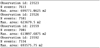 |
Fig. A.1 Output from the code example shown in Figure 3. |
| In the text | |
 |
Fig. A.2 Output from the code example shown in Figure 6. |
| In the text | |
 |
Fig. A.3 Output from the code example shown in Figure 5. |
| In the text | |
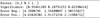 |
Fig. A.4 Output from the code example shown in Figure 8. |
| In the text | |
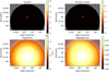 |
Fig. A.5 Output from the code example shown in Figure 7. |
| In the text | |
 |
Fig. A.6 Output from the code example shown in Figure 10. |
| In the text | |
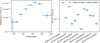 |
Fig. A.7 Output from the code example shown in Figure 11. |
| In the text | |
 |
Fig. A.8 Output from the code example shown in Figure 9. |
| In the text | |
Current usage metrics show cumulative count of Article Views (full-text article views including HTML views, PDF and ePub downloads, according to the available data) and Abstracts Views on Vision4Press platform.
Data correspond to usage on the plateform after 2015. The current usage metrics is available 48-96 hours after online publication and is updated daily on week days.
Initial download of the metrics may take a while.