| Issue |
A&A
Volume 690, October 2024
|
|
|---|---|---|
| Article Number | A250 | |
| Number of page(s) | 12 | |
| Section | Numerical methods and codes | |
| DOI | https://doi.org/10.1051/0004-6361/202451020 | |
| Published online | 11 October 2024 | |
A background-estimation technique for the detection of extended gamma-ray structures with IACTs
1
Friedrich-Alexander-Universität Erlangen-Nürnberg, Erlangen Centre for Astroparticle Physics,
Nikolaus-Fiebiger-Str. 2,
91058
Erlangen,
Germany
2
Max-Planck-Institut für Kernphysik,
Saupfercheckweg 1,
69117
Heidelberg,
Germany
★ Corresponding author; This email address is being protected from spambots. You need JavaScript enabled to view it.
Received:
7
June
2024
Accepted:
23
August
2024
Abstract
Context. Estimation of the number of cosmic-ray-induced background events is a challenging task for Imaging Atmospheric Cherenkov Telescopes (IACTs). Most approaches rely on a model of the background signal derived from archival observations, which is then normalised to the region of interest (ROI) and respective observation conditions using emission-free regions in the observation. However, this is disadvantageous for the analysis of large, extended γ-ray structures, where no sufficient source-free region can be found.
Aims. We aim to address this issue by estimating the normalisation of a three-dimensional background model template from separate, matched observations of emission-free sky regions. As a result, the need for an emission-free region in the field of view of the observation becomes unnecessary.
Methods. To this end, we implemented an algorithm to identify observation pairs with the most closely matching observation conditions. We used the open-source analysis package Gammapy to estimate the background rate, facilitating seamless adaptation of the framework to many γ-ray detection facilities. We employed public data from the High Energy Stereoscopic System (H.E.S.S.) to validate this methodology.
Results. The analysis demonstrates that employing a background rate estimated through this run-matching approach yields results consistent with those obtained using the standard application of the background model template. Furthermore, we confirm the compatibility of the source parameters obtained through this approach with previous publications, and present an analysis employing the background model template approach, along with an estimation of the statistical and systematic uncertainties introduced by this method.
Key words: methods: data analysis / gamma rays: general
© The Authors 2024
 Open Access article, published by EDP Sciences, under the terms of the Creative Commons Attribution License (https://creativecommons.org/licenses/by/4.0), which permits unrestricted use, distribution, and reproduction in any medium, provided the original work is properly cited.
This article is published in open access under the Subscribe to Open model. This email address is being protected from spambots. You need JavaScript enabled to view it. to support open access publication.
1 Introduction
Imaging Atmospheric Cherenkov Telescopes (IACTs) have considerably expanded our knowledge of the very high-energy γ-ray sky. With the advent of the upcoming Cherenkov Telescope Array (Cherenkov Telescope Array Consortium 2019, CTA), IACTs will remain a crucial tool for γ-ray astronomy for the foreseeable future. Despite this, recent results from Water Cherenkov Detectors (WCDs), such as the High-Altitude Water Cherenkov Array (Abeysekara et al. 2017, HAWC) and the Large High Altitude Air Shower Observatory (Lhaaso Collaboration 2021, LHAASO), have highlighted a limitation of IACTs. Whilst their superior angular resolution enables IACTs to distinguish between γ-ray sources situated in close proximity to one another and measure the extension of those sources with high precision, identifying large extended structures of γ-ray emission remains challenging.
This is primarily due to the effect the comparatively small field of view (FoV) of IACTs has on the detection of extended γ-ray sources (Abdalla et al. 2021). While WCDs are survey instruments that continuously monitor the overhead sky, IACTs need to be pointed towards a target source and can only observe the sky in a region of a few degrees in width. This affects the estimation of background rates in the case of studying extended source regions that cover a large part of the FoV. The background consists of extensive non-γ-ray-induced air showers, predominantly due to hadrons interacting with the Earth’s atmosphere; although at lower energies, cosmic-ray electrons also play a significant role. By implementing selection criteria on the reconstructed shower parameters (Ohm et al. 2009), this background can be significantly reduced, but not fully removed. The residual background rate is then often estimated from source-free regions in the FoV of the observation (Berge et al. 2007)1.
However, it is not always possible to find a sufficiently large source-free region, especially in the case of large, extended sources that fill a significant fraction of the FoV, which can lead to the subtraction of significant emission in the whole FoV (H.E.S.S. Collaboration 2023; Aharonian et al. 2024a; Abdalla et al. 2021). The choice of a region that is not free of gammaray emission can then lead to absorption of these structures in the background estimation. To circumvent this problem, a spec- tromorphological background model template constructed from archival data can be used, enabling a three-dimensional (3D) likelihood analysis (for more information see Mohrmann et al. 2019). Due to the large number of observations – acquired under similar conditions – used for the creation of the background model template, this approach is very stable and suffers very little from statistical fluctuations in the background estimate. Previous studies have shown that employing a background model template to estimate the background facilitates the detection of large, extended structures with IACTs (Abdalla et al. 2021). However, the background model template approach still requires a renormalisation for each observation run to account for differences in atmospheric conditions or slight hardware degradation, again requiring at least a small emission-free region in the FoV.
This problem was highlighted in a recent study of emission around the Geminga pulsar (PSR J0633+1746) with the High Energy Stereoscopic System (H.E.S.S.) (H.E.S.S. Collaboration 2023). This study revealed that while it is possible to detect the extended emission around the pulsar, an absolute measurement of its properties was not possible due to the lack of emission-free regions in the FoV (H.E.S.S. Collaboration 2023). Instead, only a relative measurement was feasible, where the background level was estimated in regions of fainter γ-ray emission.
In regions where no emission-free region can be identified, a so-called ‘ON/OFF’ approach can be used, whereby every observation of the targeted source (ON run) is matched to an observation conducted in a part of the sky that is predominantly source-free (OFF run); Abramowski et al. (2012) describe such an analysis.
This approach is a standard technique for background rejection in IACTs (Berge et al. 2007), and has already been employed by the Whipple observatory (Weekes et al. 1989). Though this standard approach can be very powerful for the observation of extended sources, because no assumptions need to be made regarding the background acceptance across the FoV, it also has major disadvantages. In the classical approach, an empty sky region needs to be observed for a comparable duration and under a similar zenith angle (with an allowed Zenith angle deviation between ON and OFF runs of typically 30′) (Berge et al. 2007; Abramowski et al. 2012). Additionally, the best description can be achieved if the OFF run is recorded shortly after the ON run, as in this case the influence of effects like degradation of the system or changes in the atmosphere is avoided. This means that, at most, half of the observation time can be spent on the actual target of the study. Additionally, a background estimate based on only one observation run is necessarily afflicted with relatively large statistical uncertainties.
In this work, we alleviate the disadvantages of both background estimation techniques by combining the classical ON/OFF method with the three-dimensional background model template constructed from archival data. For this purpose, the normalisation of the background model template for each run pair is determined from the OFF run and this normalisation is then used for the ON run. Employing this background model template differs from the classical approach, because the background rate is not estimated from just one OFF run, but many. This enables us to decrease the dependence of the background rate on the particular OFF run selected and thus to lower the uncertainty of the background estimate.
We developed this new method using the data structure of the High Energy Stereoscopic System (H.E.S.S.), an array of five IACTs located in the Khomas Highland in Namibia (Aharonian et al. 2006; Ohm et al. 2023). The original telescope array consisted of four telescopes with 12 m-diameter mirrors (CT1– 4) and was commissioned between 2000 and 2003. In 2012, a fifth telescope (CT5) with a mirror diameter of 28 m was added in the centre of the 120 m square spanned by CT1-4, lowering the energy threshold of the array considerably (van Eldik et al. 2016). The method was then validated using data from the first H.E.S.S. public data release (H.E.S.S. Collaboration 2018). As this method only requires common Python packages, as well as Gammapy (Aguasca-Cabot et al. 2023; Donath et al. 2023), it is in accordance with the goal of the Very-high-energy Open Data Format Initiative (VODF; Khelifi et al. 2023) to achieve a common, software-independent data format and develop open-source analysis software (Nigro et al. 2021). This also means that the method can easily be adapted to other telescope arrays.
Hereafter, we refer to the template constructed in Mohrmann et al. (2019) as the ‘background model template’; the standard method employed by the Whipple Observatory as the ‘classical ON/OFF method’ (Weekes et al. 1989); and the method developed in this work as the ‘run-matching approach’. With this publication, we will release the scripts necessary to perform the background matching, after a set of OFF runs has been selected, as well as the results for all spectral and spatial fits on the public-dataset release.
For this study, only data acquired by the four smaller telescopes of the H.E.S.S. array are analysed. For all observations used, the data reduction was performed using HAP, the H.E.S.S. analysis package described in Aharonian et al. 2006, and reconstructed using the Image Pixel-wise fit for Atmospheric Cherenkov Telescope algorithm ImPACT (Parsons & Hinton 2014).
Binning used for the background model template.
2 Run matching
For the classical ON/OFF method, an observation of an empty region with similar properties to that of the target region needs to be conducted. This requirement is necessary to achieve a comparable system acceptance (relative rate of events passing selection cuts). While the use of a background model template allows relaxed run-matching criteria with respect to the classical ON- OFF matching, allocating a comparable OFF run is nevertheless a critical aspect of the background estimation.
Previous works employing the classical ON/OFF method have shown that a variety of parameters influence the background rate and need to be considered in the matching process (Flinders 2016; Abeysekara 2019; H.E.S.S. Collaboration 2023; Veh 2018). In this work, an OFF run is only considered if its pointing position is at a Galactic latitude of |b| ≤ 10°, which allows us to avoid regions including many known γ-ray sources, as well as diffuse γ-ray emission. Furthermore, we only consider observations taken under good atmospheric conditions, and a good system response, and require that the same telescopes of the array participate in both the ON and OFF run. This quality selection was performed following the recommendations in Aharonian et al. (2006).
Matching parameters used for the OFF run estimation.
2.1 Matching parameters
The parameters found to have the greatest influence are the zenith angle (the angle between the pointing direction of the telescopes and zenith), changes in hardware configuration, and atmospheric conditions. The level of night sky background (NSB) light is also used for matching, because of its influence on the performance of the telescopes (Ahnen et al. 2017; Archambault et al. 2017). As small changes of the atmosphere and degradation of the system can be absorbed by the fit of the background model template (see Sect. 3), the run pairs do not need to be acquired in the same night, but can be up to a few years apart. It is however important to match runs using the same hardware configuration. Therefore, we take optical phases into account. These are periods of stable optical efficiency, between abrupt changes due to, for example, cleaning of the Winston cones (light guides attached to the camera pixels) or mirror recoating. Typically, these phases span at least one year for the H.E.S.S. telescopes, therefore enabling the choice of many possible OFF runs for one ON run. The optical phases used for this work can be found in Table A.1.
For the construction of the background model template, the zenith angles of the OFF runs were grouped into bins with a size dependent on the available statistics, because of the strong influence of the zenith angle on the background rate (Bretz 2019). The zenith angle bins from Mohrmann et al. (2019) were adopted as a validity range of the zenith angle deviation for this work in order to ensure compatibility with the background model template (see Table 1). In order to have a comparable background model template between ON and OFF runs, the azimuth angle bins from Mohrmann et al. (2019) were also adopted for this study.
Another important matching parameter is the so-called muon efficiency εμ. This quantity specifies how many photo-electrons are detected per incident photon, and is therefore a measure of the optical performance of the telescopes (Vacanti et al. 1994; Gaug et al. 2019). Its estimation through measurements on muon events becomes possible because the geometry of the muon images can be used to calculate the expected intensity, which can then be compared to the measured intensity.
To evaluate the differences in atmospheric conditions between two runs, two quantities were investigated. The first parameter is the Cherenkov transparency coefficient (Hahn et al. 2014). It describes the transparency of the atmosphere and can be calculated via:
 (1)
(1)
with the number of participating telescopes N, the average amplification gain of the photosensors ɡi, and the trigger rate Ri and muon efficiency µi of observation i. The term Δ allows for higher order corrections and kN is a scaling factor (Hahn et al. 2014). The second matching parameter is the effective sky temperature in the FoV of the individual telescopes, which is measured with infrared radiometers (Aye et al. 2003). Hereafter, this quantity is referred to as radiometer temperature.
Additionally, we require the ON and OFF runs to have a comparable dead-time-corrected observation time.
In this study, the influence of the respective matching parameters on the background estimate has been estimated by calculating the distance correlation (Székely et al. 2007) between the matching parameters and the number of background events estimated in an OFF region using the background model template. In contrast to the Pearson correlation coefficient, the distance correlation allows the correlation between two parameters to be measured independently of the nature of their correlation.
As the influence of the matching parameters can vary following major changes in the hardware configuration of the telescope array, the correlation coefficients have been calculated for each of the three hardware phases of the H.E.S.S. telescopes. HESS Phase 1 represents the data taken from the commissioning of the first four telescopes until the addition of the fifth telescope in 2012 (Aharonian et al. 2006). The data set taken with the five- telescope array is called HESS Phase 2 (Bolmont et al. 2014). The last set, called HESS Phase 1U, includes all data taken after the camera upgrade of the four small telescopes in 2017 (Giavitto et al. 2017).
For a correlation coefficient of dcorr ≥ 0.15, the influence of the matching parameter on the background rate was regarded as significant. A summary of all significant matching parameters, as well as allowed deviations and correlation coefficients for this work, can be found in Table 2.
These correlation coefficients were estimated using the number of background counts over the whole energy range. We additionally computed correlation coefficients using only low-energy events and find that there are no significant differences from the coefficients presented in Table 2.
2.2 Fractional run difference
The deviations of the matching parameters are then used to quantify the difference between an ON and OFF run, by calculating the fractional run difference ƒ:
 (2)
(2)
where j is one of the matching parameters, and dcorr,j is the distance correlation for the respective matching parameter (see Table 2). The observation with the smallest fractional run difference is chosen as the OFF run for the corresponding ON run.
If no OFF run fulfilling all matching criteria can be found, only the parameters with the largest influence (top half of Table 2) are used for the matching. In this case, the fractional run difference computed with all matching parameters can be large, and the suboptimal matching is then taken into account by increased systematic errors (as described in Sect. 4).
3 Background estimation
3.1 General method
After matching every ON run with an OFF run, the background model template was normalised to the OFF run. During this process, the background rate RBG underwent correction for minor discrepancies stemming from varying observation conditions, employing  , where E0 = 1 TeV is the reference energy, and the spectral tilt δ and background normalisation Φ are determined through a 3D likelihood fit of the background model template to an emission-free region in the OFF run (Mohrmann et al. 2019).
For every ON and OFF run, we estimated the energy at which the deviation between true and reconstructed energy – referred to as the energy bias – reaches 10%. This energy was then set as a safe energy threshold and the data at lower energies were discarded. The maximally allowed offset between the reconstructed event direction and the pointing position of the camera was 2.0°.
Gammapy version 1.2 (Aguasca-Cabot et al. 2023; Donath et al. 2023) was used to create a dataset with a square region geometry of 4° × 4° centred around the pointing position of the OFF run. This MapDataset combines information such as a counts map (the observed number of events passing selection cuts in each bin), expected background map, and exposure. The size of the geometry was chosen such that all of the data within the above-mentioned thresholds were included in the analysis. For a correct description of the amount of cosmic-ray background in the observation, it is important to ensure that no γ-ray source is present in the region to which the parameters of the background model template are fitted.
Therefore, the regions containing previously identified extragalactic γ-ray sources in the OFF run were excluded from the fit of the background model template. Additionally, we excluded a circular region with a radius of 0.5° around the observation target of the respective OFF run to minimise the amount of γ-ray emission included due to subthreshold γ-ray sources. The background model template was then fit to the OFF run. Thereafter, only the adjusted background model template was used.
In addition to minimising the deviations between ON and OFF run by comparing the fractional run deviation and identifying the best-matching OFF run, deviations between the observations can be accounted for by applying correction factors. One correction applied accounts for the deviation in duration (observation time during which the telescope system can trigger on a signal) between the ON and OFF runs:
 (3)
(3)
where bi is the total number of background events per spatial pixel and t is the total duration of the observation.
The second correction applied accounts for the deviation in zenith angle of the observation. Because of the matching within the zenith angle bins used in the computation of the background model template (see Table 1), some run pairs can have a deviation of up to 5° in zenith angle Θz. The correction factor to account for this deviation is calculated using:
 (4)
(4)
This correction follows the relation between the cosmic-ray rate – and therefore also the trigger rate, which is dominated by hadronic background events – and the zenith angle of the measurement established in Lebohec & Holder (2003). The parameters p1 and p2 were estimated for every optical phase by fitting Eq. (4) to the trigger rate of the H.E.S.S. array for all observations performed in the respective optical phase. An example of such a fit to the trigger rates can be seen in Fig. 1. The fit parameters for all optical phases, as well as more information about their computation, can be found in Appendix A.
In the next step, another MapDataset was created and filled with the reconstructed events observed in the ON run. The background model template was then assigned to this dataset, and the spectral tilt δ and background normalisation Φ derived from the fit of the template to the OFF run were assumed for this dataset. This allows us to adjust the background rate to the different observation conditions without the need to have γ-ray emission-free regions in the ON run.
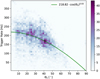 |
Fig. 1 Dependence of the array trigger rate of the four small H.E.S.S. telescopes on the zenith angle of the measurement for the first optical phase. A fit of Eq. (4) to the data yields the parameters used for the background correction. |
3.2 Creation of validation datasets
In order to validate the above-described background-estimation method, the background rate and source parameters achieved by applying the run-matching approach should be compared to the standard background model template method. To achieve this, we construct validation datasets consisting of observations of gamma-ray sources that are either point-like or exhibit only marginal extension, facilitating the application of both methods. For this purpose, different datasets for all regions of interest (ROI) around the sources were constructed in order to estimate the accuracy of the background description using the run-matching approach. For ease of reference, these different cases have been given numbers, and an overview can be found in Table 3. First, a standard analysis of all ON runs for a ROI is performed as a reference. For this purpose, all observations of the target region are identified, the background model template is fitted to each ON run, and the resulting MapDatasets are ‘stacked’, which means the measured data are summed over all observations, averaged instrument response functions (IRFs) are created, and only one MapDataset is returned for every ROI. Hereafter, this dataset is referred to as Case 0. Another dataset was constructed using the same approach, this time with the runmatching approach, but without corrections, in order to estimate the background rate. Hereafter, this is referred to as Case 1. We constructed one dataset where only the correction for the differences in duration was applied (Case 2) and another where both corrections were applied (Case 3). Two more datasets were constructed to estimate the influence of the systematic errors introduced due to the run-matching approach (see Sect. 4); these are labelled Case 4+ and Case 4- respectively for increased and decreased background count rate.
Overview of the identifiers used for the datasets in this validation.
3.3 Derivation of the correlation coefficients and validity intervals
We identified the influence of the respective matching parameters on the background rate by analysing archival H.E.S.S. data obtained for the γ-ray source PKS 2155-304 using the direct application of the background model template (Case 0).
PKS 2155-304 was chosen as a test region as it has been continuously monitored since the commissioning of the first H.E.S.S. telescope and a large amount of data with varying observation conditions has been acquired. Additionally, the γ- rays in this ROI are contained in a small, well-known region, resulting in a small uncertainty in the background rate.
The background model template was fitted to each observation in this dataset (see Sect. 3), and the number of background events was estimated. The data were then split into three groups depending on the hardware configuration of the telescope array. We used a total of 791 observations over the three hardware phases. A Pearson correlation coefficient between the different matching parameters and the background rate was then computed. The results can be seen in Table 2. To estimate the valid parameter range for every matching parameter, we compared the background rate estimated for Case 0 with that resulting from the run-matching approach (Case 3) for a large number of observations. To this end, we used all observation pairs from the sets of observations on PKS 2155–304, indicated in Table 4.
For each of these observations, all possible OFF runs were identified. We then computed the background rate of all pairs for Case 0 and Case 3, and calculated the deviation of these as follows:
 (5)
(5)
with RBG,0 the background rate of the dataset for Case 0 and RBG,3 the background rate for Case 3. Additionally, the deviation between all matching parameters of ON and OFF runs was calculated for each observation pair as Δx = (xon − xoff)/xon, where x is a given matching parameter. We then computed the mean background rate deviation  per Δx, and define the valid parameter range as the Δx at which
  . This computation is performed individually for all four telescopes, and the smallest value is identified as the upper bound of the validity range. A visualisation of the distribution of
  and its mean for the Muon efficiency can be seen in Fig. 2.
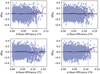 |
Fig. 2 Background rate deviation ΔRBG per difference in muon efficiency for each run pair in set 3 (see Table 5 for more information on the dataset). The case of no deviation between the background rates is depicted by the grey dashed line, and the mean of ΔRBG is depicted by the purple line. |
4 Systematic errors
In order to estimate the systematic uncertainties introduced by employing the run-matching approach, we directly compared the background rates for Case 0 and Case 3. To this end, we selected a set of observations on a well-known target region. For each of these observations, we identified all possible OFF runs, and then computed the background rate of all pairs for Case 0 and Case 3, and then calculated the deviation of these as indicated in Eq. (5). We computed this deviation, which is a measure of the systematic shift, for all run pairs and the results are grouped according to the fractional run difference of the respective OFF run. Although this comparison is a good estimation of the systematic uncertainty introduced by the run-matching approach, it is limited by the available statistics, and a coarse bin size of Δƒ = 0.1 was chosen. Subsequently, the standard deviation of the background deviation was computed in each bin with more than ten entries to ensure sufficient statistics for a stable result. The standard deviation was then used as systematic uncertainty on the background count rate for a run pair with the respective fraction run deviation.
Because of strong variations in the optical efficiency of the telescopes, the systematic uncertainty can vary for observations obtained at different times. To account for this effect, the systematic uncertainties should be computed for each individual analysis by selecting observations recorded in a short time-span around the recording of the ON runs used for the source analysis. In the present study, we used ON runs from three different time periods, and therefore three different sets of observations for the estimation of the systematic uncertainties were computed. For all three sets, we used observations on the source PKS 2155–304, excluding the observations that are part of the public data release. Table 4 provides further properties of these sets, and shows which source analyses they were used for.
A visualisation of the systematic shift for all three sets can be seen in Fig. 3. The systematic errors for set 1 and set 2 are comparable, whilst the errors for set 3 are marginally smaller. This is most likely caused by a camera update in 2016 (Giavitto et al. 2017). Set 3 also extends to higher fractional run deviations ƒ , because a greater number of observations on extragalactic sources was acquired in this time period.
The influence of this systematic shift of the background rate on the source parameters is then estimated by computing two additional datasets for each test region. For the computation of these datasets, the fractional run difference of every run pair was used to identify the systematic shift expected for this pair and the background counts per pixel were then increased and decreased using the corresponding systematic factor. These datasets are identified as Case 4+ for the increased background rate and Case 4− for the decreased background rate.
Properties of the sets of observations from which the systematic uncertainties were estimated and the corresponding source analysis they were used for.
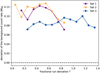 |
Fig. 3 Systematic uncertainties on the background count rate introduced by using a run-matching approach for different fractional run deviations ƒ for all datasets. The error bars represent the standard deviation of all pairs in the respective ƒ bin. A description of the respective sets can be found in Table 4 |
5 Validation
To validate the run-matching approach, we analysed data from the H.E.S.S. public dataset release (H.E.S.S. Collaboration 2018) (Case 3) and compared the results to an analysis using the background model template (Case 0) and to the results reported in Mohrmann et al. (2019). Additionally, this work uses observations of sky regions devoid of γ-ray emission (which are referred to as empty-field observations hereafter) acquired with the H.E.S.S. telescope array. We note that the archival data used for the construction of the background model template, as well as the OFF runs used for these analyses and the observations of the empty-field observations, are proprietary to the H.E.S.S. Collaboration and are not publicly available.
The public data release only contains data passing a tight quality selection (for more information, see Aharonian et al. (2006)). Therefore, all observations that are part of the data release can be used for this validation study. The empty-field observations were filtered to only contain runs taken under good atmospheric conditions. The properties of these datasets are listed in Table 5.
The spectral and morphological properties of the γ-ray emission from all sources contained in the public data release (see Table 5) were acquired by performing a three-dimensional fit of a spectromorphological model to the dataset. A ‘stacked’ analysis was performed using Gammapy, whereby the data were summed over all observations and the likelihood minimisation of the model fit parameters was carried out over averaged IRFs.
All datasets were prepared using a spatial pixel size of 0.02°. The spatial extension of the MapDatasets for each analysis region was chosen such that all events recorded in the observations were included in the analysis, and the energy axis for each dataset was chosen to be logarithmically spaced, with eight bins per decade.
5.1 Validation with empty-field observations
The quality of the background estimation was assessed via the Li & Ma (1983) significance distribution. For an empty sky region, we expect a Gaussian distribution centred around µ = 0, with a standard deviation of σ = 1, since the fluctuations of the background counts are Poisson distributed.
To test for the correct description of the background, we examined three datasets comprised of observations centred on the empty-filed regions, namely regions around the dwarf spheroidal galaxies Reticulum II, Tucana II, and Sculptor Dwarf Galaxy. These regions were chosen because no significant γ- ray emission from the sources or within a 4° region around the sources has been observed with H.E.S.S. (Abdallah et al. 2020; Abramowski et al. 2014a). Therefore, the regions can be used for an estimation of the background rate without contamination from a mismodelled γ-ray source.
For all regions, we computed the significance of the number of events passing selection cuts in excess of the background prediction. The correlation radius used for the construction of the significance maps is 0.06° for all empty-field observations, which approximately corresponds to the point-spread function of H.E.S.S. A Gaussian model is fitted to each significance distribution with the fit results for the different regions given in Table 6. An example distribution for the region around the dwarf spheroidal galaxy Tucana II, and the corresponding Gaussian fit, can also be seen in Fig. 4.
For Case 0, all three regions show a distribution centred around zero and a standard deviation of approximately 1.0, confirming that no γ-ray sources are present. The mean of the distributions for Case 1 indicates an over-prediction of cosmicray background of up to 20%. This over-prediction is slightly decreased if a duration correction is applied (Case 2), and is further reduced once the zenith correction is applied for all three empty-field regions.
The Gaussian fit to the significance histograms of these datasets shows that the nominal value derived for the Case 0 datasets is included in the range covered by the systematic error for all datasets. An example of the shift on the significance distribution caused by the inclusion of the systematic errors can be seen in Fig. 5.
We also tested the validity of the background estimation method in different energy ranges, again using the three empty-field data sets. For this purpose, the data were divided into eight logarithmically spaced energy bins, from 0.1 TeV to 10 TeV. This binning was chosen so that each bin included two energy bins of the initial dataset. The data above 10 TeV were not included in this comparison due to insufficient gamma-ray statistics. We find that for the three data sets, a Gaussian fit to the significance distribution yields comparable results between the Case 0 and Case 3 datasets in all energy bins. The mean and standard deviation for the Gaussian fits in energy bands are quoted in Wach et al. (2024, Tables B.1–B.3) and a visual example of the region around Sculptor can be seen in Wach et al. (2024, Fig. B.2)
To check for variation in background counts as a function of energy due to the run matching, we computed the background counts per energy bin for all empty-field region observations for Case 0  and Case 3
  . We then computed the ratio between these counts
  per energy bin. We find that the number of background counts for the Case 3 datasets is slightly underestimated for lower energies and slightly overestimated for higher energies compared to the number of counts derived for the Case 0 datasets. This deviation is however found to be below 6% for all energies and can be seen in Wach et al. (2024, Fig. B.1)
Analysis datasets used in this study.
Gaussian distribution of the Li & Ma (1983) significance values of the background events derived from the empty-field observations.
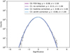 |
Fig. 4 Li & Ma (1983) significance distribution of the observations in the region around the dwarf spheroidal galaxy Reticulum II. Depicted are the distributions for four different estimates of the background; see Table 6. Each of the distributions is shown as a histogram in grey, while a Gaussian fit to each distribution is shown by the coloured lines. |
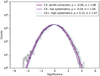 |
Fig. 5 Li & Ma (1983) significance distributions of background counts in the region around the dwarf spheroidal galaxy Tucana II for the different background estimation methods. |
5.2 Public data release
After verifying the background prediction in an empty sky region, the best-fit values for a source analysis should be verified between the different background estimation techniques. To this end, we analysed data from the public data release of H.E.S.S. (H.E.S.S. Collaboration 2018) for both background estimation methods, and compared the results to those derived in Mohrmann et al. (2019). A simple power-law was chosen as a spectral model for all datasets, and in all cases, the flux normalisation N0 at a reference energy E0 and the spectral index Γ were used as fit parameters. The power-law model is defined as:
 (6)
(6)
The reference energy for all datasets was chosen to be equal to the values used in Mohrmann et al. (2019), for the sake of comparison, and can be found in Wach et al. (2024, Table C.1)
The correlation radius used for the computation of the significance maps and histograms for all datasets is 0.06°, except the dataset centred on the Crab Nebula, which is 0.1°, because of the small size and limited statistics of the dataset.
For the sake of comparing the best-fit results between this analysis and the results obtained in Mohrmann et al. (2019), the same spatial models are chosen and should not be interpreted as yielding the most accurate description of the region. The Crab Nebula, as well as PKS 2155–304, are described using a point source model. For a more in-depth discussion of these sources, see Aharonian et al. (2024b) and H.E.S.S. Collaboration (2017), respectively. The pulsar wind nebula MSH 15–52 (analysed in detail in Aharonian et al. (2005)) is described by an elongated disc model. For the supernova remnant RX J1713.7–3946, no predefined spatial model could be used because of the complicated morphology of the source. For this reason an ‘excess template’ was constructed (for more information about the construction of this excess template, see Mohrmann et al. 2019). More information describing the emission from RX J1713.7–3946 can be found in H.E.S.S. Collaboration (2018).
An additional challenge for the analysis of these datasets is that, depending on the source location, misclassified cosmic rays are not the only source of background events. Observations centred in the Galactic plane will also include events from the Galactic diffuse emission (Abramowski et al. 2014b). For the background estimation employing the background model template, the Galactic diffuse emission can be partly absorbed by increasing the normalisation of the background model template. In the case of the run-matching approach, the background model template is normalised on observations outside of the Galactic plane, and so absorption of the diffuse emission into the background is not possible.
This effect has been observed in the analysis of the datasets centred on the regions around the sources MSH 15–52, located at a Galactic latitude of b = −1.19,° and RX J1713.7–3946, with a Galactic latitude of b = −0.47°. For both datasets, an excess signal across the whole FoV was detected at low energies. Whilst it is likely that the observed excess emission is Galactic diffuse emission, the data used in this validation are not extensive enough to model this signal or derive any of its physical properties. Therefore, we adopted a strict energy threshold for the analysis of the regions around MSH 15–52 and RX J1713.7–3946, effectively excluding the energy range in which a significant influence of diffuse emission can be observed for H.E.S.S.. This energy threshold was evaluated for each individual analysis for Case 3. To this end, we estimated the number of background and signal events in a source-free region in the stacked dataset. The first energy bin after which the absolute difference between the number of signal and background events is less than 10% was adopted as an energy threshold for the analysis. For the analysis of both MSH 15–52 and RX J1713.7–3946, this resulted in an energy threshold of 560 GeV. In addition to the increased energy thresholds, a second modification of the background estimation needs to be included for the datasets for MSH 15–52 and RX J1713.7–3946. Because they were taken in 2004, shortly after the commissioning of the H.E.S.S. array, the optical phase is very short because of the fast system degradation, and few observations were taken outside of the Galactic plane in this time period. For this reason, an insufficient number of OFF runs can be found within this optical phase and the first two optical phases have been combined.
The best-fit parameters for the datasets created using the run-matching approach for all sources can be found in Wach et al. (2024, Table C.1). Additionally, the best-fit values derived in the previous analysis are also indicated in the table for comparison, as are the results derived from the Case 0 datasets. A visual comparison of the fit parameters for all sources can be found in Appendix C.
5.2.1 Point-like sources
The comparison of the best-fit parameters for the analysis of the γ-ray emission from the Crab Nebula and PKS 21550–304 can be found in Wach et al. (2024, Appendix C). The left panel of Fig. 6 shows a significance map for the region around the Crab Nebula. Indicated in the significance map are the 5 σ and 8 σ contours for Case 3 in dashed pink lines, and the contours for Case 0 as solid blue lines. The contours show good agreement.
The right panel of Fig. 6 shows the distribution of significance entries in the respective maps. A region of 0.5° radius around the source has been excluded to avoid contamination of residual γ-ray emission from the source. The significance map and histogram of the region around PKS 2155–304 can be found in Wach et al. (2024, Fig. D.4) Figure 7. The distribution of the background counts shows a shift between the datasets for Case 0 and Case 3, indicating a slight over-prediction of the background rate for the Case 3 dataset. This shift is however within the expected range derived from a study of the influence of the systematic uncertainties (see Table 7)
The best-fit results of the likelihood minimisation for the Crab Nebula can be seen in Wach et al. (2024, Fig. C.1). All parameters except the best-fit position are comparable within statistical errors with the results derived in Mohrmann et al. (2019). The comparability of the right ascension between Case 0 and Case 3 suggests that a change in pointing reconstruction might be responsible for this deviation. A similar deviation can be observed for the best-fit parameters of PKS 2155–304 (see Wach et al. 2024, Fig. C.2), where we also see a slight decrease in flux normalisation compared to the results derived in Mohrmann et al. (2019). Good agreement is seen for both sets of SEDs depicted in Wach et al. (2024, Figs. D.1 and D.2). Only in one energy bin, around 3 TeV, is the deviation above 1 σ between the SEDs derived from the Crab Nebula. A possible reason for this deviation is the change in the binning of the background model template that has been incorporated since the publication of Mohrmann et al. (2019).
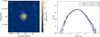 |
Fig. 6 The Region around the Crab Nebula as seen with the H.E.S.S. Telescopes. Left: Li & Ma (1983) significance map of the region with 5 σ and 8 σ contours. The contours from case 0 are depicted in blue, while the contours from case 3 are depicted in pink. The best-fit position is indicated by the black cross. Right: significance distribution of the background in the FoV. |
Gaussian distribution of the Li & Ma (1983) significance values of the background events derived for each of the datasets in the H.E.S.S. public data release.
5.2.2 MSH 15–52
A significance map of the region around MSH 15–52 can be seen in Wach et al. (2024, Fig. D.5) alongside the distribution of background. In this region, a shift of the background distribution towards a smaller number of cosmic-ray signals can be observed. This shift is most likely caused by a lack of OFF runs in this optical phase, making it necessary to choose OFF runs from the next optical phase. It is therefore possible that the time-span between the ON and OFF runs is larger than 4 years, resulting in a high probability that the optical efficiency of the telescopes between the two observations differs substantially. The shift can, however, be accounted for by the systematic uncertainty introduced by the run-matching approach.
The best-fit values for all parameters agree within the error (see Fig. 7). The strong dependence of the source extension on the correct estimation of the background rate is clearly shown by the large systematic errors, which are introduced by the systematic uncertainty on the run-matching results. The SED derived for this source shows a good agreement within the errors with the SED computed in Mohrmann et al. (2019) (see Wach et al. 2024, Fig. D.3)
5.2.3 RX J1713.7–3946
Wach et al. (2024, Fig. D.6) present a significance map and distribution for the region around RX J1713.7–3946. Good agreement between the background rate estimated for Case 0 and Case 3 is again seen.
The best-fit parameters can be seen in Wach et al. (2024, Fig. D.3). The spectral index and flux normalisation for RX J1713.7–3946 agree with the results of the likelihood minimisation within the error. A comparison of the SEDs for RX J1713.7–3946 can be seen in Fig. 8. The upper panel of the figure shows a comparison of the SED derived using the run-matching approach with that derived by Mohrmann et al. (2019), while the lower panel shows the deviation between the two sets of SEDs. Again, a good agreement can be observed.
To verify that this background estimation is also stable for a large number of observations, we analysed a dataset containing 53.4 hours of observations centred on RX J1713.7–3946. The results of this analysis reveal good agreement between Case 0 and Case 3. As this dataset is not part of the public dataset release, the SEDs and best-fit parameters are not presented in this work, but a more detailed analysis of this region using the same dataset can be found in H.E.S.S. Collaboration (2018).
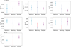 |
Fig. 7 Comparison between the best-fit values for all parameters of the elongated model used to describe the emission from MSH 15–52. The reference values were taken from Mohrmann et al. (2019). Here, ‘matching’ refers to the values derived using the run-matching approach for the background estimation, while ‘template’ refers to the background model template. The systematic uncertainties introduced when using the run-matching approach are indicated in red. |
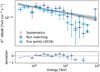 |
Fig. 8 SED of RX J1713.7–3946 derived in the present analysis compared to the SED derived by Mohrmann et al. (2019). The systematic uncertainties added by the run-matching approach are indicated in red in the upper panel. The lower panel shows the deviation between the SED derived in both analyses and the best-fit model derived from the Case 3 dataset. |
6 Conclusions
We present a method to combine the classical ON/OFF background estimation technique used by IACT arrays with a 3D background model template. This combination of techniques allows us to remove a major restriction of each method. As the 3D background model template has been created from a large number of OFF runs, it is robust and not subject to large statistical uncertainties. However, this method requires source-free regions in the FoV of the observation in order to normalise the background estimation for varying observation conditions. The classical ON/OFF background estimation does not require a source-free region, but is nevertheless very sensitive to variations in observation conditions.
Although we are able to achieve good agreement with the previously published results for all sources, the datasets used here already give an indication of the limitations of this technique. To achieve a comparable background rate between ON and OFF runs, the two need to be chosen from periods with comparable optical efficiency. Due to the limited number of available OFF runs in these periods, large systematic errors can be introduced on the source parameters. This effect can be mitigated by constructing a background model template suitable for long-term hardware conditions, with corrections to the normalisation designed to account for short-term variations, thereby expanding the pool of viable OFF runs for these periods.
While this study presents a detailed analysis of the systematic uncertainty on the run-matching approach, an additional source of uncertainty – not examined in detail here – is introduced because of the stacking of the observations. This method of combining the observations for the analysis can produce a slight gradient in the number of background counts over the FoV. While this effect is small, it should nevertheless be kept in mind when interpreting the results achieved with this method and becomes particularly relevant for large, extended sources.
An additional problem of this framework is how to treat the Galactic diffuse emission. In this work, we increased the energy threshold to exclude the influence of the diffuse emission, but this is not ideal. A better approach would be to construct an additional spectromorphological template from interstellar gas tracers.
While these disadvantages show that the run-matching approach presented here cannot compete with the 3D background model template method in regions containing few sources with a small extension, the non-dependence on source-free regions in the observation is a major advantage in sky regions with many sources or for the detection of diffuse extended structures, which cannot be observed using the background model template alone. The presented background-estimation technique is an extension of the background estimation using a 3D background model template, offering the possibility to still profit from the small statistical uncertainty of the background model template, even for regions filled with significant emission, where this method can traditionally not be used. This application is vital considering that there are currently no Water Cherenkov Detectors observing the southern γ-ray sky, restricting the observable source population to structures that can be detected with the comparatively small FoV of the H.E.S.S. array. The combined method presented here also has the potential to increase the population of sources observable with CTA, opening up the possibility of using the superior angular resolution to expand our knowledge of large extended structures previously uniquely detected by the Water Cherenkov Detectors.
Data availability
Additional visualisation of the results derived in this study, as well as the scripts necessary to perform the background matching, after a set of OFF runs has been selected, and the results for all spectral and spatial fits on the public-dataset release can be found at https://doi.org/10.5281/zenodo.13684196.
Acknowledgements
This work made use of data supplied by the H.E.S.S. Collaboration. We would like to thank the H.E.S.S. Collaboration, especially Stefan Wagner, Spokesperson of the Collaboration, as well as Nukri Komin, chair of the Collaboration Board, and Markus Boettcher, Chair of the Publication Board, for allowing us to use the data presented in this publication. We also gratefully acknowledge the computing resources provided by the Erlangen Regional Computing Center (RRZE). This work was supported by the German Deutsche Forschungsgemeinschaft, DFG project number 452934793.
Appendix A Zenith angle correction
To account for differences in mean zenith angle of the observation between ON and OFF run, Eq. (4) was fitted to the array trigger rates in every optical phase. The resulting fit parameters are given in Table A.1.
Zenith angle correction to the background rate for different optical phases.
References
- Abdalla, H., Aharonian, F., Ait Benkhali, F., et al. 2021, ApJ, 917, 6 [NASA ADS] [CrossRef] [Google Scholar]
- Abdallah, H., Adam, R., Aharonian, F., et al. 2020, Phys. Rev. D, 102, 062001 [NASA ADS] [CrossRef] [Google Scholar]
- Abeysekara, A. 2019, in International Cosmic Ray Conference, 36, 36th International Cosmic Ray Conference (ICRC2019), 616 [NASA ADS] [Google Scholar]
- Abeysekara, A. U., Albert, A., Alfaro, R., et al. 2017, ApJ, 843, 39 [NASA ADS] [CrossRef] [Google Scholar]
- Abramowski, A., Acero, F., Aharonian, F., et al. 2012, A&A, 548, A38 [NASA ADS] [CrossRef] [EDP Sciences] [Google Scholar]
- Abramowski, A., Aharonian, F., Ait Benkhali, F., et al. 2014a, Phys. Rev. D, 90, 112012 [NASA ADS] [CrossRef] [Google Scholar]
- Abramowski, A., Aharonian, F., Ait Benkhali, F., et al. 2014b, Phys. Rev. D, 90, 122007 [NASA ADS] [CrossRef] [Google Scholar]
- Aguasca-Cabot, A., Donath, A., Feijen, K., et al. 2023, https://doi.org/10.5281/zenodo.8033275 [Google Scholar]
- Aharonian, F., Akhperjanian, A. G., Aye, K. M., et al. 2005, A&A, 435, L17 [NASA ADS] [CrossRef] [EDP Sciences] [Google Scholar]
- Aharonian, F., Akhperjanian, A. G., Bazer-Bachi, A. R., et al. 2006, A&A, 457, 899 [NASA ADS] [CrossRef] [EDP Sciences] [Google Scholar]
- Aharonian, F., Ait Benkhali, F., Aschersleben, J., et al. 2024a, A&A, 686, A149 [NASA ADS] [CrossRef] [EDP Sciences] [Google Scholar]
- Aharonian, F., Ait Benkhali, F., Aschersleben, J., et al. 2024b, A&A, 686, A308 [NASA ADS] [CrossRef] [EDP Sciences] [Google Scholar]
- Ahnen, M. L., Ansoldi, S., Antonelli, L. A., et al. 2017, Astropart. Phys., 94, 29 [NASA ADS] [CrossRef] [Google Scholar]
- Archambault, S., Archer, A., Benbow, W., et al. 2017, Astropart. Phys., 91, 34 [NASA ADS] [CrossRef] [Google Scholar]
- Aye, K. M., Chadwick, P. M., Hadjichristidis, C., et al. 2003, in International Cosmic Ray Conference, 5, 2879 [NASA ADS] [Google Scholar]
- Berge, D., Funk, S., & Hinton, J. 2007, A&A, 466, 1219 [CrossRef] [EDP Sciences] [Google Scholar]
- Bolmont, J., Corona, P., Gauron, P., et al. 2014, Nucl. Instrum. Methods Phys. Res. A, 761, 46 [CrossRef] [Google Scholar]
- Bretz, T. 2019, Astropart. Phys., 111, 72 [Google Scholar]
- Cherenkov Telescope Array Consortium (Acharya, B. S., Agudo, I., et al.) 2019, Science with the Cherenkov Telescope Array [Google Scholar]
- Donath, A., Terrier, R., Remy, Q., et al. 2023, A&A, 678, A157 [NASA ADS] [CrossRef] [EDP Sciences] [Google Scholar]
- Flinders, A. 2016, in Proceedings of The 34th International Cosmic Ray Conference – PoS(ICRC2015), 236, 795 [CrossRef] [Google Scholar]
- Gaug, M., Fegan, S., Mitchell, A. M. W., et al. 2019, ApJS, 243, 11 [NASA ADS] [CrossRef] [Google Scholar]
- Giavitto, G., Bonnefoy, S., Ashton, T., et al. 2017, in International Cosmic Ray Conference, Vol. 301, 35th International Cosmic Ray Conference (ICRC2017), 805 [NASA ADS] [Google Scholar]
- Hahn, J., de los Reyes, R., Bernlöhr, K., et al. 2014, Astropart. Phys., 54, 25 [NASA ADS] [CrossRef] [Google Scholar]
- H.E.S.S. Collaboration 2018, https://doi.org/10.5281/zenodo.1421099 [Google Scholar]
- H.E.S.S. Collaboration (Abdalla, H., et al.) 2017, A&A, 598, A39 [NASA ADS] [CrossRef] [EDP Sciences] [Google Scholar]
- H.E.S.S. Collaboration (Abdalla, H., et al.) 2018, A&A, 612, A6 [NASA ADS] [CrossRef] [EDP Sciences] [Google Scholar]
- H.E.S.S. Collaboration (Aharonian, F., et al.) 2023, A&A, 673, A148 [NASA ADS] [CrossRef] [EDP Sciences] [Google Scholar]
- Khelifi, B., Zanin, R., Kosack, K., Olivera-Nieto, L., & Schnabel, J. 2023, PoS, ICRC2023, 1510 [Google Scholar]
- Lebohec, S., & Holder, J. 2003, Astropart. Phys., 19, 221 [NASA ADS] [CrossRef] [Google Scholar]
- Lhaaso Collaboration (Cao, Z., et al.) 2021, Science, 373, 425 [Google Scholar]
- Li, T. P., & Ma, Y. Q. 1983, ApJ, 272, 317 [CrossRef] [Google Scholar]
- Mohrmann, L., Specovius, A., Tiziani, D., et al. 2019, A&A, 632, A72 [NASA ADS] [CrossRef] [EDP Sciences] [Google Scholar]
- Nigro, C., Hassan, T., & Olivera-Nieto, L. 2021, Universe, 7, 374 [NASA ADS] [CrossRef] [Google Scholar]
- Ohm, S., van Eldik, C., & Egberts, K. 2009, Astropart. Phys., 31, 383 [NASA ADS] [CrossRef] [Google Scholar]
- Ohm, S., Wagner, S., & H. E. S. S. Collaboration 2023, Nucl. Instrum. Methods Phys. Res. A, 1055, 168442 [CrossRef] [Google Scholar]
- Parsons, R. D., & Hinton, J. A. 2014, Astropart. Phys., 56, 26 [Google Scholar]
- Rowell, G. P. 2003, A&A, 410, 389 [NASA ADS] [CrossRef] [EDP Sciences] [Google Scholar]
- Székely, G. J., Rizzo, M. L., & Bakirov, N. K. 2007, Ann. Statist., 35, 2769 [Google Scholar]
- Vacanti, G., Fleury, P., Jiang, Y., et al. 1994, Astropart. Phys., 2, 1 [NASA ADS] [CrossRef] [Google Scholar]
- van Eldik, C., Holler, M., Berge, D., et al. 2016, in Proceedings of The 34th International Cosmic Ray Conference – PoS(ICRC2015), 236, 847 [CrossRef] [Google Scholar]
- Veh, J. 2018, PhD thesis, Erlangen Centre for Astroparticle Physics (ECAP), Friedrich-Alexander-Universität Erlangen-Nürnberg, Germany [Google Scholar]
- Wach, T., Mitchell, A., & Mohrmann, L. 2024, https://doi.org/10.5281/ zenodo.13684196 [Google Scholar]
- Weekes, T. C., Cawley, M. F., Fegan, D. J., et al. 1989, ApJ, 342, 379 [NASA ADS] [CrossRef] [Google Scholar]
Another approach, initially proposed by Rowell (2003), is to estimate the background rate from a separate set of events that are more cosmic-ray-like than the selected gamma-ray candidates. However, this approach requires detailed knowledge about the acceptance of the system to these cosmic-ray-like events, and is not discussed further in this work.
All Tables
Properties of the sets of observations from which the systematic uncertainties were estimated and the corresponding source analysis they were used for.
Gaussian distribution of the Li & Ma (1983) significance values of the background events derived from the empty-field observations.
Gaussian distribution of the Li & Ma (1983) significance values of the background events derived for each of the datasets in the H.E.S.S. public data release.
All Figures
|
Fig. 1 Dependence of the array trigger rate of the four small H.E.S.S. telescopes on the zenith angle of the measurement for the first optical phase. A fit of Eq. (4) to the data yields the parameters used for the background correction. |
| In the text | |
|
Fig. 2 Background rate deviation ΔRBG per difference in muon efficiency for each run pair in set 3 (see Table 5 for more information on the dataset). The case of no deviation between the background rates is depicted by the grey dashed line, and the mean of ΔRBG is depicted by the purple line. |
| In the text | |
|
Fig. 3 Systematic uncertainties on the background count rate introduced by using a run-matching approach for different fractional run deviations ƒ for all datasets. The error bars represent the standard deviation of all pairs in the respective ƒ bin. A description of the respective sets can be found in Table 4 |
| In the text | |
|
Fig. 4 Li & Ma (1983) significance distribution of the observations in the region around the dwarf spheroidal galaxy Reticulum II. Depicted are the distributions for four different estimates of the background; see Table 6. Each of the distributions is shown as a histogram in grey, while a Gaussian fit to each distribution is shown by the coloured lines. |
| In the text | |
|
Fig. 5 Li & Ma (1983) significance distributions of background counts in the region around the dwarf spheroidal galaxy Tucana II for the different background estimation methods. |
| In the text | |
|
Fig. 6 The Region around the Crab Nebula as seen with the H.E.S.S. Telescopes. Left: Li & Ma (1983) significance map of the region with 5 σ and 8 σ contours. The contours from case 0 are depicted in blue, while the contours from case 3 are depicted in pink. The best-fit position is indicated by the black cross. Right: significance distribution of the background in the FoV. |
| In the text | |
|
Fig. 7 Comparison between the best-fit values for all parameters of the elongated model used to describe the emission from MSH 15–52. The reference values were taken from Mohrmann et al. (2019). Here, ‘matching’ refers to the values derived using the run-matching approach for the background estimation, while ‘template’ refers to the background model template. The systematic uncertainties introduced when using the run-matching approach are indicated in red. |
| In the text | |
|
Fig. 8 SED of RX J1713.7–3946 derived in the present analysis compared to the SED derived by Mohrmann et al. (2019). The systematic uncertainties added by the run-matching approach are indicated in red in the upper panel. The lower panel shows the deviation between the SED derived in both analyses and the best-fit model derived from the Case 3 dataset. |
| In the text | |
Current usage metrics show cumulative count of Article Views (full-text article views including HTML views, PDF and ePub downloads, according to the available data) and Abstracts Views on Vision4Press platform.
Data correspond to usage on the plateform after 2015. The current usage metrics is available 48-96 hours after online publication and is updated daily on week days.
Initial download of the metrics may take a while.