| Issue |
A&A
Volume 678, October 2023
|
|
|---|---|---|
| Article Number | A192 | |
| Number of page(s) | 24 | |
| Section | Planets and planetary systems | |
| DOI | https://doi.org/10.1051/0004-6361/202346442 | |
| Published online | 24 October 2023 | |
Size-dependent charging of dust particles in protoplanetary disks
Can turbulence cause charge separation and lightning?
1
Austrian Academy of Science, Space Research Institute,
Schmiedlstrasse 6,
8042
Graz,
Austria
e-mail: This email address is being protected from spambots. You need JavaScript enabled to view it.
2
TU Graz, Faculty of Mathematics, Physics and Geodesy,
Petersgasse 16,
8010
Graz,
Austria
3
Centre for ExoLife Sciences (CELS), Niels Bohr Institute,
Østervoldgade 5,
1350
Copenhagen,
Denmark
4
Max Planck Institute for Extraterrestrial Physics,
Giessenbachstrasse 1,
85748
Garching,
Germany
Received:
16
March
2023
Accepted:
1
August
2023
Abstract
Context. Lightning can have a profound impact on the chemistry of planetary atmospheres. In a similar manner, as protoplanetary disks are the foundation of planet formation, the emergence of lightning in protoplanetary disks can substantially alter their chemistry.
Aims. We aim to study under which conditions lightning could emerge within protoplanetary disks.
Methods. We employed the PRODIMO code to make 2D thermo-chemical models of protoplanetary disks. We included a new way of how the code handles dust grains, which allows the consideration of dust grains of different sizes. We investigated the chemical composition, dust charging behavior, and charge balance of these models to determine which regions could be most sufficient for lightning.
Results. We identify six regions within the disks where the charge balance is dominated by different radiation processes and find that the emergence of lightning is most probable in the lower and warmer regions of the midplane. This is due to the low electron abundance (nе/n〈H〉 < 10−15) in these regions and dust grains being the most abundant negative charge carriers (nZ/n〈H〉 > 10−13). We find that NH4+ is the most abundant positive charge carrier in those regions at the same abundances as the dust grains. We developed a method of inducing electric fields via turbulence within this mix of dust grains and NH4+. The electric fields generated with this mechanism are however several orders of magnitude weaker than required to overcome the critical electric field.
Key words: protoplanetary disks
© The Authors 2023
 Open Access article, published by EDP Sciences, under the terms of the Creative Commons Attribution License (https://creativecommons.org/licenses/by/4.0), which permits unrestricted use, distribution, and reproduction in any medium, provided the original work is properly cited.
This article is published in open access under the Subscribe to Open model. This email address is being protected from spambots. You need JavaScript enabled to view it. to support open access publication.
1 Introduction
Dust grains in protoplanetary disks play a crucial role in disk evolution and planet formation (see, e.g., reviews by Lesur et al. 2023, Drazkowska et al. 2023). The dust grains in the midplane tend to pick up free electrons, which changes the character of the chemistry and has been shown to be connected to the degree of ionization (Bai & Stone 2011; Ivlev et al. 2016). Thus, grain charges are important for dust dynamics and instabilities, such as the magneto-rotational instability (MRI; see, e.g., Salmeron & Wardle 2008; Perez-Becker & Chiang 2011; Bai 2011; Thi et al. 2019). Additionally, grain charges and MRI can play an important role in and can be used for explaining gap formations in a disk, as shown in Dullemond & Penzlin (2018), Regály et al. (2021, 2023).
Dust grains accumulate toward the midplane via gravitational settling, enhancing the concentrations of the large grains in particular (see, e.g., Dubrulle et al. 1995; Dullemond & Dominik 2004; Riols & Lesur 2018). Dust grains undergo growth as well, where the charge of the grains can play an important role. Dust grains tend to uniformly charge negatively in the shielded midplane regions, which can create an electrostatic repulsion between the grains large enough to prevent collisions and hence growth. This effect is known as the “charge barrier” (see, e.g., Okuzumi 2009; Okuzumi et al. 2011, and Akimkin et al. 2020).
In this work, we investigate if charged dust grains can trigger discharge phenomena similar to lightning on Earth. Lightning is a universal phenomenon that occurs in the atmospheres of several different types of astrophysical objects. Most prominently, lightning occurs in Earth’s atmosphere, and due to the high temperatures (Orville 1968a,b,c) associated with it, lightning has several implications on the Earth’s atmospheric chemistry. Lightning also plays a central role in the abiotic fixation of nitrogen (Noxon 1976; Hill et al. 1980), which is the creation of several nitrogen bearing species, such as NOx (Price et al. 1997), from elemental nitrogen N2. Nitrogen fixation via lightning is also central in the prebiotic fixation of nitrogen (Navarro-González et al. 2001), a process which made nitrogen available to the first lifeforms on Earth. Further implications of this process are the abundance of ozone in Earth’s atmospheres, as ozone is a product of reactions between NOx and elemental oxygen (Wild 2007; Murray et al. 2013). Lightning is not just a prominent feature of Earth, and it has been observed on other planets and moons in the Solar System. The Pioneer Venus Orbiter missions revealed lightning discharges on Venus from clouds in the ionosphere (Russell et al. 2006, 2007, 2008), and the potential chemical implications have been discussed by Delitsky & Baines (2015). Cassini revealed that lightning also occurs on Saturn (Baines et al. 2009; Dyudina et al. 2010).
There has also been a vast amount of work on the theoretical front, including discussions on the existence of lightning on objects such as brown dwarfs (Helling et al. 2016; Hodosán et al. 2016) and exoplanets (Méndez Harper et al. 2018; Helling & Rimmer 2019). The findings of these discussions have revealed that lightning is a phenomenon that is ubiquitous. There has also been a significant amount of work contributed to answer the question of whether lightning is feasible in protoplanetary disks. Lightning induced by triboelectric or collisional charging could be a reasonable mechanism in forming chondrules, as shown by Desch & Cuzzi (2000). The triboelectric charging they implemented in their work is not considered in this work. Similar work has been done in Muranushi (2010), who calculated a critical dust number density at which lightning should occur. Compared to our present work, they are missing an explicit turbulence analysis. In the realm of lightning in disks, one should also mention the works of Inutsuka & Sano (2005), Okuzumi & Inutsuka (2015), and Okuzumi et al. (2019). In particular, the latter two investigate how dust grains charge in weakly ionized plasma and additionally study the heating of dust grains by electric fields, which are induced via magneto hydrodynamics (MHD). This work differs in the way electric fields are generated. They investigated how MRI could induce electric fields that heat the dust grains, while we investigate Kolmogorov turbulence. In addition, no MHD effects are considered in this work. We find that we should also mention Johansen & Okuzumi (2017), as they argue that lightning discharge can be caused by positron emission from pebbles that contain radioactive Al26. In our work, the main source of ionization is cosmic rays, and we do not consider radioactive decay. In order for lightning to emerge, certain conditions have to be met. Charges need to build up and then have to be separated, and this separation and buildup have to result in a large enough electric field for an electron cascade to occur (Williams 1985; Gurevich & Zybin 2005; Saunders 2008). In clouds on the Earth, the charges are built-up by ice crystals becoming charged via collisions with each other (Takahashi 1978; Jayaratne et al. 1983; Saunders 1993; Saunders & Peck 1998). During these collisions, faster growing and therefore smaller particles tend to charge positively, whereas the larger particles charge negatively (Baker et al. 1987; Dash et al. 2001). For charge separation in clouds, an updraft is generally required, and in this updraft, a lower positive layer and an upper negative layer form (Stolzenburg et al. 1998; Bruning et al. 2007). Another way for lightning to emerge on Earth is during volcanic eruptions (Brook et al. 1974; Gaudin et al. 2018). While the fundamentals are similar to lightning in clouds, some (important) details are different. In volcanic eruptions, dust particles in the volcanic plumes are the particles that become triboelectrically charged (Houghton et al. 2013). Triboelectric charging leads to the smaller particles becoming charged more negatively and larger particles being charged more positively (Lacks & Levandovsky 2007; Forward et al. 2009).
Lastly, one should also mention the new experimental findings in triboelectric charging by Jungmann & Wurm (2021) and Wurm et al. (2022). In the first publication, Jungmann and Wurm state that triboelectric charging could be instrumental in overcoming the bouncing barrier, and in the second, the authors investigate how triboelectric charging could play a role in ionizing the gas phase. The former explanations might lead the reader to ask whether the conditions in protoplanetary disks can lead to a similar emergence of lightning. We think so, as the collection of dust in high densities found in the midplane of protoplanetary disks due to gravitational settling resembles conditions found on Earth and other planets, moons, and even brown dwarfs where lightning has been shown to emerge. In addition to this, turbulent motions, which could result in charge separation, are found in protoplanetary disks.
In Sect. 2, we explain our model, which includes explanations on the chemistry of our code, all the numerical basics and improvements we have done to our code, and how we implemented cosmic rays. In Sect. 3, we present the results of our simulations. In particular, we investigate the role electrons play in our simulations, how the dust grains become charged, and whether specific regions of the disk can be favorable for the emergence of lightning. We furthermore investigate how turbulent eddies could induce a charge separation in these areas and if electric fields that emerge from this separation could be large enough for lightning to emerge. In Sect. 4, we summarize our results. We provide a glossary of the different symbols used in this work in Table A.1.
2 The thermo-chemical disk model
To simulate the size-dependent charging of dust grains in a protoplanetary disk, we used the Protoplanetary Disk Model (PRODIMO) developed by Woitke et al. (2009, 2016). PRODIMO is a 2D thermo-chemical disk modeling code that combines detailed continuum and line radiative transfer with the solution of a chemical network, the determination of the non-local thermal equilibrium (LTE) population of atomic and molecular states, and the heating-cooling balance for both gas and dust.
The model uses a simple parametric density setup chosen to represent a 2 Myrs old T Tauri star. All further assumptions about the star; the disk shape; the irradiation of the disk with FUV photons, X-rays, and cosmic rays; the dust material composition and opacities; and dust settling are explained in detail in Woitke et al. (2016, see their Table 3). Here, in this publication, we only explain the changes made to the PRODIMO code that differ from the code used in Woitke et al. (2016), and differences to the setup from Woitke et al. (2016). The selected values for the stellar, disk shape, and dust parameters are summarized in Table 3.
2.1 Chemical setup
We choose the so-called large DIANA-standard chemical network with 235 species as our base network for this work. It has been described in detail by Kamp et al. (2017). Most UV, cosmic ray, two-body, and three-body reaction rates are from the UMIST 2012 database (Woodall et al. 2007; McElroy et al. 2013). In addition, there are rates for the H2 formation on grains, reactions for electronically excited molecular hydrogen  , polyaromatic hydrocarbon (PAH) charge chemistry (Thi et al. 2019), and a simple freeze-out chemistry for the ice phases of all neutral molecules (see Woitke et al. 2009; Kamp et al. 2017). The large DIANA-standard network also includes X-ray processes with doubly ionized species from Aresu (2012).
We added a number of dust species to this base chemical network to represent the different charging states q of grains of different sizes a. By solving the chemical rate network, we determined the dust charge distribution function for every given size and charge f(a, q) from which we could then compute, for example, the mean charge of grains of different sizes, including the feedback of the charged grains on all other results of the chemistry.
In contrast to Woitke et al. (2016), we have chosen to omit the PAH charging states in the chemistry in this paper, but PAH heating is still taken into account. If present, the PAHs can introduce similar effects as charged grains. Since we want to study the chemical feedback of charged grains in disks in particular, we wanted to avoid any confusion between PAH charging and dust charging. In addition, preliminary tests showed that the impact of PAHs in the midplane is negligible, due to the PAHs freezing out. Therefore, we also omitted them to lower the numeric effort.
2.2 Dust size distribution and settling
In PRODIMO, the dust component enters into the modeling (i) as an opacity source for the continuum, (ii) its effect on line radiative transfer, and (iii) as a set of chemical species that can pick up and release charges in the chemical rate network. The dust grains, however, are neither created nor destroyed, nor do they grow in the chemistry module.
Our assumptions about dust settling and opacity are explained in Woitke et al. (2016). The dust size distribution function before settling [cm−1] is assumed to be
 (1)
(1)
which is the same everywhere in the disk, using Nsize log-equidistant size grid points between the minimum grain radius amin and the maximum radius amax. The proportionality constant in Eq. (1) is derived from the local gas density ρ(r, z), the dust material density ρgr, and the global gas-to-dust mass ratio, assumed to be 100 in this paper. In each vertical column at radius r, all grains of size a are vertically redistributed with a scale height that is smaller than the gas scale height. Here, in this publication, we used the settling description by Dubrulle et al. (1995) with the settling parameter αsettle = 0.01, as outlined in Woitke et al. (2016). After applying the settling, the dust size distribution function f(a, r, z) is numerically available on the Nsize size grid points at each point (r, z) in the model. The term f(a, r, z) is the basis for the opacity calculations.
2.3 Dust size bins in the chemistry
We used a much smaller number of dust size bins Nbin (between two and nine) to represent the position-dependent dust size distribution function after settling f(a, r, z) in the chemistry. The idea in this section is to introduce two power-law indices, κ and ζ, to make the sparse representation exact with regard to two selectable dust size moments. We then argue which of the dust size moments should be selected in order to minimize the numerical errors in the chemistry introduced by the sparse resolution of f(a, r, z) in size space. We start by computing the following moment of the dust size distribution function
 (2)
(2)
where f(a, r, z) [cm−1] is normalized as  . For example, ζ = 2, nd 4π 〈a2〉 is the total dust surface per cubic centimeter [cm2 cm−3]. Next, we divide 〈aζ〉 by Nbin and numerically adjust the bin boundaries aj such that each size bin contains the same portion of 〈aζ〉.
 (3)
(3)
Here, aj terms are the size bin boundary values, where a0 = amin and  . Once the aj are fixed this way, we compute similar quantities
 (4)
(4)
and define the average size of our grains [cm] in the dust bin j as
 (5)
(5)
Finally, the dust particle densities [cm−3] in the size bin j are calculated as
 (6)
(6)
From Eqs. (3) to (6), it follows that

which means that our dust bins {(nd,j āj) | j = 1, … , Nbin) exactly represent two dust size moments where the dust size distribution function is weighted with aκ and aζ, respectively (see Table 1).
If κ = 0 is chosen, the quantity 〈aκ〉j becomes the fraction of dust particles having sizes between aj−1 and aj, and consequently, the total dust number density  becomes exact. In a similar way, choosing ζ = 2 causes the representation of the total dust surface to be exact. All other dust size moments, however, show deviations from their true integral values. Increasing the number of dust bins Nbin would reduce these problems.
Thus, with κ and ζ, we can choose two dust size moments that are represented exactly by the bins and are most relevant for the problem at hand. Since the effects of the charged grains in the chemistry, via their collisional and photoionization rates, scale with their total cross-section, a choice of ζ = 2 seems appropriate. That scaling, however, is not exact because there are second-order dependencies of the rates on grain charge over radius q/a (see Sect. 2.8). In addition, the conservation of the total charge is an important principle. The total number of elementary charges on the grains per volume, assuming q/a = const is valid (see Sect. 2.8), is
 (7)
(7)
Therefore, it seems important to get the first dust size moment correct as well. In contrast, there is no direct link between the total dust particle density and the chemistry nor to any dependencies of the chemistry on the total dust volume. Therefore, our default choice is κ = 1 and ζ = 2.
Table 1 shows that in this case, we only need to represent the smaller grains up to a few microns in size. A larger value of ζ would also come with an increased level of computational problems and computing time, for example, because we would need to extend the maximum number of charging states qmax to many thousands for large grains (see Sect. 2.8).
Construction of dust size bins for the chemistry.
2.4 Dust charging reactions
The charging of dust grains is part of the chemistry of PRODIMO. We focus only on the most relevant reactions here. A full description of all considered dust grain charging processes can be found in Thi et al. (2019). The three most important reaction types are electron attachment, photoionization, and charge exchange between dust grains and molecular ions.
Photoionization. Photoionization describes the process of stripping away electrons from the dust grains via photons with sufficiently high energies.
 (8)
(8)
where Z and Z+ stand for grains with charges q and q + 1, respectively. Here, q can have any integer value greater than zero.
For positively charged and neutral grains, this process is called photoejection, and for negatively charged grains, this process is called photodetachment. According to Weingartner & Draine (2001), the energy threshold for photoejection is
 (9)
(9)
where IP is the ionization potential of the dust grain and W0 the work function of silicate grains, assumed to be 8 eV by Cuzzi et al. (2001) after measurements of Feuerbacher & Fitton (1972). The term Wc is an additional term that is dependent on the charge of the grain, and it increases the ionization potential for positive grains, making it harder to ionize the grain or decreasing the ionization potential and making it easier to ionize the grain. This additional term, Wc, is defined as
 (10)
(10)
where q is the charge of the grain normalized by the elementary charge, e is the elementary charge, and a is the grain radius. We note that the factor 1/2 is still open for discussion according to Wong et al. (2003), where a factor of 3/8 was proposed. For photodetachment, the threshold photon energy hvpd is equal to the grain electron affinity EA plus the minimum energy Emin at which the tunneling probability becomes relevant.
 (11)
(11)
 (12)
(12)
![Mathematical equation: $ {E_{\min }}\left( {q,a} \right) = - \left( {q + 1} \right){{{e^2}} \over a}{\left[ {1 + {{\left( {{{27{\rm{{\AA}}}} \over a}} \right)}^{0.75}}} \right]^{ - 1}}, $](/articles/aa/full_html/2023/10/aa46442-23/aa46442-23-eq21.png) (13)
(13)
where Ebg is the band gap, assumed to be 5 eV in Weingartner & Draine (2001); a is the dust grain radius; and q is the grain charge in units of the electron charge. For the total rate coefficient of photoionization, one has to combine both photodetachment and photoejection. The rate coefficient therefore takes the form of
 (14)
(14)
where Jν is the direction-averaged flux of photons per area and second [cm−2s−1]; νpe is the threshold frequency of photoejection; νpd is the threshold frequency for photodetachment; νmax is the maximum frequency of photons, being equivalent to an energy of 13.6eV in PRODIMO; Qabs is the frequency-dependent absorption efficiency; ηeff and ηpd are the yields of the photoejection and photodetachment (Weingartner & Draine 2001) of silicate; and a is the dust grain radius.
Electron attachment. The rate coefficient for electron attachment,
 (15)
(15)
is derived by averaging over the Maxwellian velocity distribution of the impinging electrons. Here Z and Z− stand for grains with charges q and q − 1, respectively, where q can have any integer value less than or equal to zero. This results in a reaction coefficient ke(q) of the form
 (16)
(16)
where ne is the electron density, Se is a sticking coefficient assumed to be larger than 0.3 (Umebayashi & Nakano 1980) and set to 0.5 in our simulations, T is the gas temperature, me is the electron mass, and kb is the Boltzmann constant. The dust grain cross-section is represented by σZ = πa2, and a is the dust grain radius. The term fq is a charge-dependent factor that is derived by taking the Coulomb interaction between the incoming electron and charged grain into account. For neutral grains, we have fq = 1. For positively charged grains (q > 0), there is an additional attraction that enlarges the rate, and for negatively charged grains (q < 0), there is Coulomb repulsion
 (17)
(17)
Charge exchange. Dust grains can get charged via charge exchanges between dust grains and molecular ions. The most prevalent charge exchange for this study is the exchange of a negative charge between a negatively charged dust grain and a positively charged molecular ion,
 (18)
(18)
The general form of the rate coefficient is similar to the electron attachment. Since we only allowed for exothermal charge exchange reactions, the rate coefficient takes the form
 (19)
(19)
where, analog to Eq. (17),
 (20)
(20)
where nM is the density of the molecules, qM is the charge of the impinging molecule (usually +1), SM is a sticking coefficient set to one (Thi et al. 2019), nM is the number density of the molecule, and mM is the molecular mass.
We note that we excluded passive ion attachment in our network. Meaning, in our network, molecules and dust grains cannot attach to each other via electromagnetic forces only. We discuss the potential implications of including passive ion attachment in Sect. 5.
We excluded endotherm charge exchange reactions between protonated molecules and dust grains, where the work function minus the band gap plus the proton affinity of the molecule exceeds 13.6 eV (see Appendix D and Table 2). In order to identify these endotherm charge exchange reactions, we needed to know the heat of formation of negatively charged dust grains  , which is given by the work function minus the band gap plus small correction terms of order e2/a (see Appendix D). In our model, we consider porous silicate grains internally mixed with amorphous carbon (see Table 3), but these grains can also be ice coated. For pure silicate grains, values for the work function minus the bad gap lie between about 3 eV and 8 eV (Weingartner & Draine 2001). Yet, following the explanations of Helling et al. (2011) and looking at the compiled values of work functions of different dust components from Desch & Cuzzi (2000) and Kopnin et al. (2004), a value between 2 eV and 6 eV seems appropriate. In this paper, we use
  , where q < 0 for negative grains, 0 for neutral grains and q > 1 for positive grains, in accordance with Thi et al. (2019). This is supported by Rosenberg (2001), who stated that a mixture of dust grain material tends to lower the work function overall. According to the data collected by Thi et al. (2019), water ice (coated) grains should have higher work functions. We can assume that our dust grains are water ice coated according to D’Angelo et al. (2019), who showed that at temperatures of 300 – 500 K, a water layer should be found on dust grains. This is further supported by Thi et al. (2020), who showed, with a PRODIMO model similar to ours, that phyllosilicates can be found in the midplane of a protoplanetary disk.
2.5 Chemical network adjustment for charge and proton exchange reactions
Particular to this work is that the code has the ability to automatically generate all possible charge exchange reactions between molecules and dust grains and proton exchange reactions between molecules and then add them to the network if they meet certain criteria. In addition, we allowed the code to add endothermic reactions to the network if they meet a predetermined requirement. We tested the implications of the different networks this creates in Appendix B.
Proton exchange reactions. Proton reactions come in the following form:
 (21)
(21)
where M1 and M2 are neutral molecules while M1H+ and M2H+ are the corresponding protonated molecules. We started our procedure by first identifying pairs of molecules and their protonated counterpart (M1, M2H+). If a reaction for the pair already exists in the network, we simply moved on. However, if a reaction between the pair was not found in the network, we added an approximated reaction to the network with certain assumptions.
The aim was to create a reaction rate with the Arrhenius equation,
 (22)
(22)
where T0 refers to the reference temperature of 293 K. In order to achieve this, we had to provide the different factors α, β, and γ. For α and β, we find their values with the following method. For each unprotonated molecule, M1, we counted how many protonation reactions for M1 already exist in the network. We summed up the different αi and βi parameters of the existing reactions. We averaged the summed-up parameters by simply dividing them by the number of reactions found in the network, nreac:
 (23)
(23)
 (24)
(24)
If we only found one reaction, we assumed αmean to be 5 × 10⁻¹⁰ and βmean to be -0.5. We then checked pairs of unprotonated and protonated molecules (M1, M2H+) and created reaction rates with the calculated αmean and βmean and the corresponding product (M1H+, M2). Lastly, we needed to calculate γ given by the reaction enthalpy ∆Hr (Eq. (25)). This was done by taking the difference of the heats of formation of the products and reactants  , with data taken from measurements at 0 K from Millar et al. (1997).
 (25)
(25)
Here, two cases can arise. In case of an exothermic reaction (∆Hr < 0), we can just add the reaction and set γ = 0. In case of an endothermic reaction (∆Hr > 0), the reaction is only added when ∆Hr/kb is smaller than a predetermined barrier. In cases where ∆Hr is small enough, γ is set to ∆Hrand the reaction is added anyway. In our standard case, we exclude endothermic reactions (i.e., we set the barrier to zero). In the appendix we investigate the impact of such endothermic reactions by using a barrier value of 5000 K.
Charge exchange reactions – molecules. For charge exchange reaction, we assume two types: non-dissociative and dissociative. We followed the same approach as with the proton exchanges, meaning we had to supply the different parameters of the Arrhenius equation. Our approach for γ is the same as with the proton exchange reactions. We calculated the difference of the formation enthalpies dHf and added it as γ if the reaction was exothermic or below the predetermined barrier. For α and β we simply assumed the values of 5 × 10⁻¹⁰ and -0.5, respectively.
Charge exchange reactions – Dust. If dust grains were involved in a charge exchange reaction, we adjusted the rate coefficient according to
 (26)
(26)
Here, A is the first factor in the Arrhenius equation and taken from the results from Leung et al. (1984), who calculated these rates for the reference dust particle density nd,ref = 2.64 × 10⁻¹² cm−3 and reference grain radius aref = 0.1 μm.
Proton affinities PA and reaction enthalpies with negatively charged silicate grains ∆Hr of selected molecules M.
Parameters of the PRODIMO disk model used in this paper.
2.6 Dust charge moments
In principle, each charge state q of the grains in size bin j could be included in the chemical rate network. However, since micron-sized grains can already collect thousands of elementary charges (Stark et al. 2015; Tazaki et al. 2020), this method would mean including a couple thousand species, which is computationally very challenging. In order to avoid this problem, the dust grains and all their charge states are represented by three charge moments,  ,
,  , and
, and  , in each size bin j.
![Mathematical equation: $ \left[ {Z_{{\rm{m,}}j}^ + } \right] = {n_{{\rm{d,}}j}}\sum\limits_{q = 1}^{{q_{\max }}} {\left( { + q} \right){f_j}\left( q \right)} $](/articles/aa/full_html/2023/10/aa46442-23/aa46442-23-eq46.png) (27)
(27)
![Mathematical equation: $ \left[ {Z_{{\rm{m,}}j}^ - } \right] = {n_{{\rm{d,}}j}}\sum\limits_{q = - {q_{\max }}}^{ - 1} {\left( { - q} \right){f_j}\left( q \right)} $](/articles/aa/full_html/2023/10/aa46442-23/aa46442-23-eq47.png) (28)
(28)
![Mathematical equation: $ \left[ {{Z_{{\rm{m,}}j}}} \right] = {n_{{\rm{d,}}j}}{q_{\max }} - \left[ {Z_{{\rm{m,}}j}^ - } \right] - \left[ {Z_{{\rm{m,}}j}^ + } \right], $](/articles/aa/full_html/2023/10/aa46442-23/aa46442-23-eq48.png) (29)
(29)
where qmax is the maximum number of elementary charges on the dust grains, both positive and negative, and nd,j is the dust number density of bin j. The moments  and
and  express the total number of positive and negative charges on the dust grains in size bin j per volume, respectively. The neutral moment Zm,j is defined in such a way that it becomes zero when all grains have a maximum charge, qmax or −qmax, and stays positive for any other charge distribution function fj(q). The charge distribution function was normalized to one (i.e., ∑ fj(q) = 1). According to Eq. (29), we can identify a constant quantity,
![Mathematical equation: $ { \in _{{Z_j}}} = {{{q_{\max }}{n_{{\rm{d,}}j}}} \over {{n_{\left\langle {\rm{H}} \right\rangle }}}} = {{\left[ {Z_{{\rm{m,j}}}^ + } \right] + \left[ {{Z_{{\rm{m}}{\rm{.j}}}}} \right] + \left[ {Z_{{\rm{m,j}}}^ - } \right]} \over {{n_{\left\langle {\rm{H}} \right\rangle }}}}, $](/articles/aa/full_html/2023/10/aa46442-23/aa46442-23-eq51.png) (30)
(30)
which we used in PRODIMO to define a quasi-element abundance for the dust grains in size bin j. Here, n〈H〉 refers to the total number density of hydrogen nuclei. The mean charge of the grains in size bin j is
![Mathematical equation: $ \left\langle {{q_j}} \right\rangle = \sum\limits_{ - q{ & _{\max }}}^{ - 1} {q{f_i}\left( q \right) + \sum\limits_1^{{q_{\max }}} {q{f_i}\left( q \right) = {{\left[ {Z_{{\rm{m,}}j}^ + } \right] - \left[ {Z_{{\rm{m,}}j}^ - } \right]} \over {{n_{{\rm{d,}}j}}}}.} } $](/articles/aa/full_html/2023/10/aa46442-23/aa46442-23-eq52.png) (31)
(31)
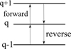 |
Fig. 1 Sketch of the linear chain of reactions that populate and depopulate the charge states q. A forward reaction adds a positive charge, a reverse reaction adds a negative charge. |
2.7 Solving for the charge distribution function
To determine the discrete charge distribution function fj(q) for all charge states q in every size bin j, we employed a method called linear chains of reactions. We note that we assumed the charge distribution function to be in a steady state. The general idea is that in our model, the charge states q of a grain can only change by one increment, either forward to q + 1 or the reverse to q − 1 . This is illustrated in Fig. 1.
The processes that add a charge, q → q + 1, are photoionization (called photoejection for neutral grains and photodetachment for negative grains) and charge exchange between a dust grain and a molecular cation. The forward rates [1/ s] were calculated in the following way:
 (32)
(32)
Here, nM is the volume density of the molecule M that interacts in a charge exchange reaction with the dust grain Z.
Processes that decrease the charge, q + 1 → q, include the recombination with electrons and charge exchange reactions with molecular anions. The reverse rates were calculated as
 (33)
(33)
After determining the processes of the forward and reverse rates, the charge distribution function fj(q) could be determined, separately in each size bin, in a step-down approach. We set fj(qmax) = 1 and performed a sequence of steps where we calculated fj(q) from fj(q +1) until q = −qmax was reached. During each step, we used
 (34)
(34)
Eventually, we calculated the normalization constant as
 (35)
(35)
and normalized it as fj(q) → fj(q)/fj,norm.
The results only depend on the UV to optical photon fluxes, the electron density ne, and the molecular ion densities M. In Fig. 2, we show the resulting fj(q) for six dust size bins at two positions in the disk. The left side of the figure shows a point in the midplane at r = 0.1 au and z = 0, and in the right side, a point in the upper areas of the disk also with r = 0.1 au but with z = 0.29 au is shown.
In the midplane, all grains charge up negatively because there are no UV-photons here, and the rate coefficients for electron attachment are larger than the rate coefficients for charge exchange with molecular ions. In addition, grains charge up negatively because free electrons have a higher mean thermal speed than molecular ions, that is,  . The lower part of the figure shows that the resulting equilibrium charge scales about linear with grain size because it is the electric potential q/a that enters into the rate coefficients. For example, all grains continue to charge up negatively until the rate for electron attachment, with decreases exponentially with q/a, balances the rates for charge exchange with molecular ions, which also depend on q/a. As a result, we get similar q/a values for all grain sizes. This behavior can also be seen and has been discussed in Okuzumi (2009). There, the authors showed that the shape of the charge distribution function is approximately Gaussian, with its width scaling with the square root of the grain size (compare to our Fig. 2). An overview of the behavior of the charge distribution function for the whole simulation, instead of examples at single points in the simulation (as seen in Fig. 2), can be seen in Fig. 3.
2.8 Effective rates in the chemical rate network
In order to solve the chemical network with the dust charge moments as species, as introduced in Sect. 2.6, we needed to derive the effective rate coefficients for the moments. We only demonstrate the derivations for the most relevant processes here. For a full description of all reactions that concern dust grains and their moment representation, we refer to Appendix C of Thi et al. (2019). For photoejection and photodetachment,
 (36)
(36)
 (37)
(37)
we have
![Mathematical equation: $\matrix{ {{{d\left[ {Z_{{\rm{m,}}j}^ + } \right]} \over {dt}} = {k_{{\rm{m,}}j,{\rm{ph}}}}\left[ {{Z_{{\rm{m,}}j}}} \right] = {n_{{\rm{d}}{\rm{.}}j}}\sum\limits_0^{{q_{\max }} - 1} {{k_{j,{\rm{ph}}}}\left( q \right){f_j}\left( q \right)} } \cr {{{d\left[ {Z_{{\rm{m,}}j}^ + } \right]} \over {dt}} = k_{{\rm{m,}}j,{\rm{ph}}}^ - \left[ {Z_{{\rm{m,}}j}^ - } \right] = {n_{{\rm{d}}{\rm{.}}j}}\sum\limits_{ - {q_{\max }}}^1 {{k_{j,{\rm{ph}}}}\left( q \right){f_j}\left( q \right)} .} \cr }$](/articles/aa/full_html/2023/10/aa46442-23/aa46442-23-eq60.png)
We note that these effective rates represent all photoreactions from charge state (q) to charge state (q + 1 ), not just for the neutral and negatively charged grains. To gain the effective rate coefficient, we divided by [Zm,j] and ![Mathematical equation: $\left[ {{\rm{Z}}_{{\rm{m,}}j}^ - } \right]$](/articles/aa/full_html/2023/10/aa46442-23/aa46442-23-eq61.png) , respectively:
, respectively:
![Mathematical equation: $ {k_{{\rm{m,}}j,{\rm{ph}}}} = {{{n_{{\rm{d,}}j}}} \over {\left[ {{Z_{{\rm{m,}}j}}} \right]}}\sum\limits_0^{{q_{\max }} - 1} {{k_{j,{\rm{ph}}}}\left( q \right){f_j}\left( q \right)} $](/articles/aa/full_html/2023/10/aa46442-23/aa46442-23-eq62.png) (38)
(38)
![Mathematical equation: $ k_{{\rm{m,}}j,{\rm{ph}}}^ - = {{{n_{{\rm{d,}}j}}} \over {\left[ {Z_{{\rm{m,}}j}^ - } \right]}}\sum\limits_{ - {q_{\max }}}^{ - 1} {{k_{j,{\rm{ph}}}}\left( q \right){f_j}\left( q \right).} $](/articles/aa/full_html/2023/10/aa46442-23/aa46442-23-eq63.png) (39)
(39)
In the code, once fj(q) has been determined as explained in Sect. 2.7, we computed ![Mathematical equation: $\left[ {{\rm{Z}}_{{\rm{m,}}j}^ + } \right]$](/articles/aa/full_html/2023/10/aa46442-23/aa46442-23-eq64.png) ,
, ![Mathematical equation: $\left[ {{{\rm{Z}}_{{\rm{m,}}j}}} \right]$](/articles/aa/full_html/2023/10/aa46442-23/aa46442-23-eq65.png) , and
, and ![Mathematical equation: $\left[ {{\rm{Z}}_{{\rm{m,}}j}^ - } \right]$](/articles/aa/full_html/2023/10/aa46442-23/aa46442-23-eq66.png) according to Eqs. (27) to (29) and then determined the effective photo rates from fj(q) by Eqs. (38) and (39). The rate coefficients are hence fully determined by the discrete charge distribution functions fj(q).
according to Eqs. (27) to (29) and then determined the effective photo rates from fj(q) by Eqs. (38) and (39). The rate coefficients are hence fully determined by the discrete charge distribution functions fj(q).
For the electron attachment, two new rate coefficients had to be derived. The derivation is analogous to the photo processes, but one has to consider the different charge states of the grains:
 (40)
(40)
 (41)
(41)
As the positively charged grains enhance the electron attachment, we needed to describe their behavior with the rate coefficient  . Neutral grains do not show this kind of enhancement; therefore, we defined another rate coefficient km,j,e. We also included the contribution of negatively charged grains to the rate for the neutral grains, even though their contribution to the overall rate coefficient is low. For positive charged grains and neutral grains, with the added contribution of negatively charged grains, we could define
![Mathematical equation: $\matrix{{{{d\left[ {Z_{m,j}^ - } \right]} \over {dt}} = {k_{m,l,{\rm{e}}}}\left[ {{Z_{m,j}}} \right] = {n_{{\rm{d}},j}}\left( {{k_{j,{\rm{e}}}}\left( 0 \right){f_j}\left( 0 \right) + \sum\limits_{ - {q_{\max }}}^{ - 1} {{k_{j,e}}\left( q \right){f_j}\left( q \right)]} } \right)} \hfill \cr {{{d\left[ {Z_{m,j}^ - } \right]} \over {dt}} = k_{m,j,{\rm{e}}}^ + \left[ {Z_{m,j}^ + } \right] = \sum\limits_1^{{q_{\max }}} {{k_{j,e}}\left( q \right){f_j}\left( q \right)} .} \hfill \cr }$](/articles/aa/full_html/2023/10/aa46442-23/aa46442-23-eq70.png)
Here, kj,e(q) are the rate coefficients for the individual charge states defined by Eq. (16). The effective rate coefficients for electron attachment are hence
![Mathematical equation: $ {k_{m,j,{\rm{e}}}} = {{{n_{{\rm{d}},j}}} \over {\left[ {{Z_{m,j}}} \right]}}\left( {{k_{j,{\rm{e}}}}\left( 0 \right){f_j}\left( 0 \right) + \sum\limits_{ - {q_{\max }} + 1}^{ - 1} {{k_{j,e}}\left( q \right){f_i}\left( q \right)} } \right) $](/articles/aa/full_html/2023/10/aa46442-23/aa46442-23-eq71.png) (42)
(42)
![Mathematical equation: $ k_{m,j,{\rm{e}}}^ + = {{{n_{{\rm{d}},j}}} \over {\left[ {{Z_{m,j}}} \right]}}\sum\limits_1^{{q_{\max }}} {{k_{j,e}}\left( q \right){f_i}\left( q \right)} . $](/articles/aa/full_html/2023/10/aa46442-23/aa46442-23-eq72.png) (43)
(43)
The charge exchange reactions between dust grains and molecules also had to be adjusted. We considered the rates for neutral grains and negative grains separately:
 (44)
(44)
 (45)
(45)
This resulted in the following charge exchange rates:
![Mathematical equation: $ {{d\left[ {Z_{{\rm{m}},j}^ + } \right]} \over {dt}} = k_{{\rm{m}},j,{\rm{ex}}}^M\left[ {{Z_{{\rm{m}},j}}} \right]\left[ {{M^ + }} \right] = {n_{{\rm{d}},j}}\left[ {{M^ + }} \right]\sum\limits_0^{{q_{\max }} - 1} {k_{j,{\rm{ex}}}^M\left( q \right){f_i}\left( q \right)} $](/articles/aa/full_html/2023/10/aa46442-23/aa46442-23-eq75.png) (46)
(46)
![Mathematical equation: $ {{d\left[ {{Z_{{\rm{m}},j}}} \right]} \over {dt}} = k_{{\rm{m}},j,{\rm{ex}}}^{M, - }\left[ {Z_{{\rm{m}},j}^ - } \right]\left[ {{M^ + }} \right] = {n_{{\rm{d}},j}}\left[ {{M^ + }} \right]\sum\limits_{ - {q_{\max }}}^{ - 1} {k_{j,{\rm{ex}}}^M\left( q \right){f_i}\left( q \right)} , $](/articles/aa/full_html/2023/10/aa46442-23/aa46442-23-eq76.png) (47)
(47)
from which we derived the rate coefficients for charge exchange with molecule M+:
![Mathematical equation: $ k_{{\rm{m,}}j,{\rm{ex}}}^M = {{{n_{{\rm{d,}}j}}} \over {\left[ {{Z_{{\rm{m,}}j}}} \right]}}\sum\limits_0^{{q_{\max }} - 1} {k_{j,{\rm{ex}}}^M\left( q \right){f_i}\left( q \right)} $](/articles/aa/full_html/2023/10/aa46442-23/aa46442-23-eq77.png) (48)
(48)
![Mathematical equation: $ k_{{\rm{m,}}j,{\rm{ex}}}^{M{,_ - }} = {{{n_{{\rm{d,}}j}}} \over {\left[ {Z_{{\rm{m,}}j}^ - } \right]}}\sum\limits_{ - {q_{\max }}}^{ - 1} {k_{j,{\rm{ex}}}^M\left( q \right){f_i}\left( q \right)} . $](/articles/aa/full_html/2023/10/aa46442-23/aa46442-23-eq78.png) (49)
(49)
With these effective rate coefficients for the dust charge moments, we could either solve our rate network system for the time-independent solution, or we could advance the ordinary system of first-order differential equations (ODE system) in time from an initial vector of particle densities. Appendix C explains how to deal with the problem that arises because fj(q) depends on the electron and molecular ion densities and the rate coefficients depend on particle densities.
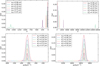 |
Fig. 2 Overview of the charge distribution function fj(q). The two upper panels show the charge distribution function in relation to the charge held by each dust grain bin q. The lower panels also show the charge distribution function but in relation to total charge per dust grain bin size Q/a. The two left panels show the result at r = 0.1 au and in the midplane at z/r = 0 for each of the six different bins. The two right panels show the results also at r = 0.1 but higher up in the disk, at z/r = 0.3 Additionally, we show the size of each bin represented by a. |
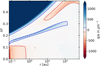 |
Fig. 3 Illustration of how the charge per dust grain radius (q/a) [μm−1 ] changes within the whole disk. For large areas of the disk, the dust is mostly neutral. In the upper areas that are largely affected by photodissociation, we find that dust charges very positively (> 100, blue contour lines). In the areas of the midplane closest to the star, we find that the dust charges very negatively (< −100, red contour lines). |
2.9 Cosmic ray implementation
As explained in Sect. 3, we expected lightning to occur, if at all, in the dense and shielded midplane regions of the disk close to the star, where cosmic rays are the most relevant source for ionization. It was therefore important to use a model for the cosmic ray penetration that is as realistic as possible.
We used the description of cosmic ray attenuation and ionization following Padovani et al. (2009) and as implemented by Rab et al. (2017, Rab et al. 2018). According to this model, the H2 cosmic ray ionization rate ζcr s−1 is given by
 (50)
(50)
where N〈H〉 [cm−2] is the vertical hydrogen nuclei column density and Σ ≈ (1.4 amu) N〈H〉 [g cm−2] the vertical mass column density. The fitting parameters are represented by ζlow, ζhigh, Σ0, and a. These fitting parameters originate from the fitting of cosmic ray spectra and account for different attenuations at different column densities. The term ζ1ow is used to fit the spectra for low column densities smaller than 1019 cm−2, where the attenuation can be described as a power law, and ζhigh is used for column densities higher than 1019 cm−2, where the attenuation can be described with an exponential term. Additionally, Eq. (50) is applied twice in our models (once to account for cosmic rays impacting the disk from above and once to account for cosmic rays impacting the disk from below) by adjusting N〈H〉 = 2N〈H〉(r, 0) − N〈H〉(r, z), where N〈H〉(r) is the total vertical hydrogen nuclei column density at point r and N〈H〉 (r, z) is the local hydrogen nuclei column density at the point (r, z) for which the cosmic ray ionization rate has to be determined. In our main simulation, we made use of the cosmic ray spectra named Solar Max in Cleeves et al. (2013). We do not include stellar energetic particles (SEPs) in this work.
3 Resulting dust charge and ionization properties
This section summarizes our results concerning the mean charge of the dust grains, how the grain charge distribution function depends on the position in the disk and on dust size, and how the dust charge is linked to the degree of ionization and molecular ions in the gas, with particular emphasis on the midplane regions. We first illustrate our standard case, where we only generated exchange reactions but no new protonation reactions and only considered exothermic reactions. A full discussion can be found in Appendix B. These results are used later to discuss whether charge separation and lightning can occur in disks (see Sect. 4). An overview of the hydrogen nuclei density and resulting radial and vertical extinction can be seen in Fig. 4. Additionally, an overview of the temperature structure can be seen in Fig. 5.
3.1 Electron concentration
Figure 6 shows the resulting electron concentration ne/n〈H〉 as a function of position (r, z) in our disk model. On the basis of these results, we introduced six different disk regions, A-F (see Fig. 6), where the physical and chemical processes leading to ionization and dust charge are qualitatively different in each case.
3.2 Regions F, E, and D – the plasma regions
Regions D–F in Fig. 6 are radiation dominated regions, where the UV and X-ray photons create a large degree of ionization along with positive dust charges. We found that region F is dominated by the ionization of H and H2, region E is dominated by the ionization of atomic carbon, and region D by the ionization of atomic sulfur. According to the assumed element abundances of H, C, and S in our disk model, the degree of ionization in regions F, E, and D is about 1, 10−4, and 10−7, respectively. The grains charge up positively via photo-effect, Z + hv → Z+ + e−, and their charge is balanced by electron recombination, Z+ + e− → Z. The total number of charges on the grains, however, is insignificant in comparison to the number of free electrons and positive ions in the gas phase. Any dynamical displacement of the charged grains would easily be balanced out by slight motions of the free electrons in the gas, making charge separations very unlikely to occur in these plasma regions (see further discussion in Sect. 4).
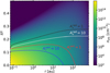 |
Fig. 4 Hydrogen nuclei density n〈H〉 [cm−3] as a function of radius r and height over the midplane z in our disk model. The different colored lines represent the visual extinctions in the radial direction (white and black) measured from the star outward and in the vertical direction (red and blue) measured from the surface of the disk toward the midplane. |
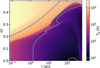 |
Fig. 5 Calculated gas temperature structure in the disk model Tg(r,z). Colored lines show different orders of magnitude in Kelvin. |
3.3 Region A – the dust dominated region
We define region A as the disk region where the number of negative charges on the dust grains is balanced by the abundance of molecular cations. Free electrons are very rare in this region (degree of ionization 10−18… 10−14) and unimportant for the charge balance. In our disk model, region A is the area that stretches out from just behind the inner rim to about r ≈ 1 au and z/r ≲ 0.1. The outer boundary coincides with the location where water and ammonia ice emerge (snowline), and the upper boundary is roughly given by a vertical visual extinction of  , which makes sure that UV photons cannot penetrate into region A.
Figure 7 shows that we found  to be by far the most important molecular cation in region A. The chemical processes that lead to this kind of charge balance in region A are multi-staged and illustrated in Fig. 8.
Since region A is entirely shielded from UV photons and X-rays, cosmic rays are found to be the only relevant ionization source, in particular
 (51)
(51)
While the free electrons are quickly picked up by the dust grains via Z + e− → Z−, the H2+ molecules, after fast reactions with H2, form the molecular cation H3+, which has a relatively low proton affinity (see Table 2). Therefore, the surplus protons in H3+ are quickly passed on to other abundant molecules, creating more complex molecular cations, such as H3O+, HCNFT, and NH4+. Further proton exchange reactions with abundant neutrals tend to increase the abundances of the protonated molecules, which have the highest proton affinities.
The NH4+ molecule has an extremely high proton affinity of 8.9 eV, which means that it cannot recombine and dissociate on grain surfaces, that is, the reaction  Η is energetically forbidden. This creates a dead end in which the concentration of
  is enhanced until an equilibrium is established with the dissociative recombination reaction
  with the extremely rare free electrons.
However, the other protonated molecules below the threshold shown in Table 2, denoted by MH+ in Fig. 8, can dissociatively recombine on the surface of the negatively charged dust grains, which creates a charging balance for the dust grains via the following three reactions:
 (52)
(52)
 (53)
(53)
 (54)
(54)
where M is the neutral abundant molecules and MH+ is their protonated counterparts, in particular H3O+ and HCNH+ in region A. There are also some simple charge exchange reactions with atomic ions A+, such as Mg+ and Fe+, whereas the electron affinity of Na+ of 5.14 eV is too small to detach an electron from a silicate grain on impact (work function 8 eV). We therefore eliminated the reaction  Na from our databases. None of the chemical reaction rates visualized in Fig. 8 involve activation barriers, which is important to remember when using this reaction scheme to discuss how the charge balance between Ζ−, MH+, NH4+, and e− reacts to any changes in density, CRI rate, or temperature. However, reaction (52) depends on the number of negative charges already collected by the grains, which is hence a result of the model.
Figure 7 shows that NH4+ remains the most abundant molecular cation up to a radial distance of about 0.7 au, which coincides with the formation of ammonia ice in the midplane of our disk model. At this point, NH3 is no longer an abundant molecule, and protonated silicon monoxide SiOH+ takes over the role of proton keeper from NH4+. The proton affinity of SiOH+ is 8.1 eV, which means that it also cannot recombine dissociatively on negatively charged dust grain surfaces. Eventually, SiO freezes out as well, at 0.9 au, and we transit into region B.
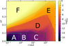 |
Fig. 6 Electron concentration ne/n〈H〉 as a function of position in the disk. We highlight areas, A-F, where the character of the chemical processes leading to grain charge and gas ionization are different (see text). |
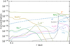 |
Fig. 7 Concentrations ni/n〈H〉 of selected chemical species important for the charge balance in the midplane in region A. The dotted blue line represents the concentration of negative charges on all dust grains |
![Mathematical equation: ${{\rm{Z}}^ - } = \sum\nolimits_j {\left[ {Z_{{\rm{m,}}j}^ - } \right]} $](/articles/aa/full_html/2023/10/aa46442-23/aa46442-23-eq82.png)
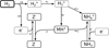 |
Fig. 8 Reaction diagram showing how the gas is ionized and the grains obtain negative charges in region A. |
3.4 Region Β – the intermediate region
We identify region Β as the disk region where the concentrations of (1) negative charges on dust grains, (2) free electrons, and (3) molecular cations are all of the same order, that is, ≈ 10−13. This happens in a transition region between about 1 au and 3 au in our disk model (see Fig. 9). Again, we required  , ruling out photoionization, which corresponds to z/r ≲ 0.1 in our disk model.
Figure 10 shows the stepwise freeze-out of oxygen, nitrogen, and carbon into ices with an outward falling temperature, which happens mostly in region B. The freeze-out starts with water ice, then ammonia ice around 1 au, and eventually several hydrocarbon ice phases, such as C3H2#, C2Hs#, and C2H4# farther out. At the end of this ice formation zone, at a distance of about 3 au, the midplane is virtually devoid of any molecules other than H2, He, noble gases, and some sulfur molecules, such as H2S, CS, and H2CS.
Therefore, the transition region Β is carbon rich, with oxygen and nitrogen already being strongly depleted by ice formation. Among the remaining hydro-carbon molecules in region B, we found Cyclopropenylidene C3H2 to have the highest proton affinity (see Table 2). Consequently, the reaction diagram in Fig. 8 would need two slight modifications for to be valid for Region Β as well. Firstly, one needs to replace NH4+ by C3H3+, because C3H3+ takes over its role as proton keeper. Secondly, we would replace M with H2S,CS and H2CS.
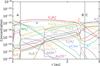 |
Fig. 9 Same plot as Fig. 7 but for region B. The dashed black lines illustrate the transition between the regions A and Β and between Β and C, respectively. |
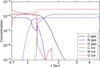 |
Fig. 10 Total abundances of oxygen, carbon, and nitrogen in gas molecules and ice phases. |
3.5 Region C – the metal-poor region
In region C (Fig. 11), there are almost no molecules other than H2 left in the gas phase because nearly all the oxygen, carbon, nitrogen, and sulfur is in the ice. Since the various electron recombination rates scale with n2 but the cosmic ray ionization rate scales with n, the electron density steadily increases toward larger radii, whereas the concentration of negative charges on dust grains Ζ− stays about constant. In fact, we used ne = [Z−] to set the boundary between regions Β and C, which happens at about 3 au in our model.
Consequently, we observed a charge equilibrium between free electrons and H3+ in region C, with some traces of F+, whereas the negatively charged dust grains became increasingly unimportant for the charge equilibrium. Toward the outer edge of region C, the disk becomes vertically transparent again, some interstellar UV and scattered UV starlight reaches the midplane, and we found increasing amounts of ionized sulfur in the gas phase. At a radial distance of about 100 au in our model, F+ and S+ become more abundant than H3+, and we enter region D.
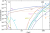 |
Fig. 11 Same as Fig. 7 but with the species that dominate the charge balance in regions C and D. The vertical dashed lines indicate the transitions between regions Β and C and between C and D. |
3.6 Dependence of grain charge on physical parameters
In order to investigate the charging behavior of dust grains in more detail, we wanted to investigate the trends seen in Fig. 2 further and see how they react to the changing of parameters that influence dust, gas, and electron abundance. In order to do this, we changed five specific parameters and studied how the affected species reacted to these changes. We changed the cosmic ray intensity ζ, the minimum dust grain size amin, the total gas density ρ, the dust-to-gas ratio, and the dust temperature Td. We did this by changing the parameters compared to our standard case (Table 3) and solved the chemistry only at the point in our simulation with r = 0.1 au and z/r = 0 in the midplane. An overview of the parameter space for each changed parameter can be found in Table 4. We only ever changed one parameter at a given time, and the other unchanged parameters remained equivalent to our standard case.
The main results of this section can be found in Fig. 12. Through the plots in the figure, we investigate the abundances of the three species that are the most influential to the charge balance at the investigated point and how the charge distribution function, as seen in the lower parts of Fig. 2, compared to qj/a, changes when varying the different parameters. In order to see changes in the charge distribution functions compared to qj/a, we created these plots for every dust bin of the different simulations. In order to make a comparison feasible, we took an average of the peaks of these charge distribution functions since Fig. 2 already revealed a very uniform behavior between the different dust bins. In addition, we calculated the standard deviations of the different qj/a values σj. These standard deviations were averaged as well, and this average can be seen in Fig. 12 as the gray shaded areas. In the following paragraphs, we describe the different subplots of Fig. 12 for each parameter in more detail.
Minimal dust size. For testing the influence of the minimum dust size on the dust charging behavior, we tested five different minimum dust sizes, starting with amin = 0.05 μm, which is the default value of our standard simulation, and increasing by a factor of ten at each step until we reached amin = 500 μm. The first big trend we observed was the decrease of the abundance of the negatively charged dust grains. This is due to the smaller surface area that a few large dust grains have, compared to many smaller ones, since one of the main contributors to the abundance of negatively charged dust grains is the total surface area. This resulted in lower rate coefficients and therefore less negatively charged dust grains, as they react less with electrons. This also explains the two other trends we observed: an increase in electron abundance and a decrease in  abundance until a saturation is reached at amin = 50 μm. As explained before, this is due to the lower amount of dust grains. Dust grains are the main reaction partner of electrons, resulting in the normally high amount of negatively charged dust grains. If fewer dust grains react with electrons, one gets more free electrons.
These free electrons are also part of the main destruction path for the  , which explains the decrease of the
  molecules. Both the electrons and the
  abundances converge toward each other because the dust grain abundance becomes fully negligible with a sufficiently high minimum dust grain size.
Dust-to-gas ratio. We tested the influence of different dust-to-gas ratios by simulating five different dust-to-gas ratios, starting with 10−4 and again increasing at each step by a factor of ten up to a dust-to-gas ratio of one. The clear trend that can be seen is the decrease of the electron abundance with increasing dust-to-gas ratios. To understand these results, it is central to remember the role dust grains play in the midplane chemistry. Dust grains are the main reaction partner of free electrons. Therefore, increasing the amount of dust grains by increasing the dust-to-gas ratio decreased the amount of electrons. Secondly, as mentioned in the last paragraph, the main destruction pathway of  molecules is via reaction with free electrons. Hence, a reduction of electrons via having more dust grains resulted in an increase of the
  molecules as well.
Cosmic rays. To investigate the impact different cosmic ray ionization rates have on our results, we chose to simulate six different cosmic ray ionization rates from ζ = 10−16 to ζ = 10−22. We note that we assumed a constant cosmic ray ionization rate, in contrast to the method we chose for our large simulations. This was done to make it easier to compare results. At the point we investigated, the cosmic ray ionization rate for our standard case is 5 × 10⁻²⁰.
The strongest trend one can see is the strong relation between the abundance of the electrons and the cosmic ray ionization rate. The trend is that the lower the cosmic ray ionization rate is, the lower the amount of electrons. This is caused by the fact that the main source of electrons in these highly shielded regions is the ionization of molecular hydrogen via cosmic rays.
We also saw no change in the abundance of  and negative charged dust grains. This is the case because the cosmic ray ionization rate also influences how many
  molecules are available. A decrease in cosmic ray ionization rate also results in less molecular hydrogen ionization. This results in a constant abundance of both negative dust grains and
  since there is a decrease of the species that are influential for both the creation and destruction of negatively charged dust grains and
  . For negatively charged dust grains, the important creation and destruction species are electrons for the creation and protonated molecules for the destruction. For
  it is the opposite.
Gas density. To see if changing the gas density changes our result, we simulated different models with a differing disk mass. As the amount of gas in our model cannot be directly increased or decreased, we had to change the disk mass instead, which indirectly increases or decreases the gas density. We simulated five different disk masses, varying from 10−4 M⊙ up to 1 M⊙. We note, however, that we plotted against gas density and not disk mass. The results are very similar to what we got from the runs where we varied the cosmic ray ionization rate, and this is because increasing the gas density also increases the shielding and hence decreases the amount of cosmic ray ionization and therefore free electrons. Thus, the effects mentioned in the previous section mostly hold true for this part as well.
Dust temperature. We further wanted to investigate how changing the dust temperature could influence the charging behavior of the grains. Thus, we changed the dust temperature from 100 K to 1800 K in steps of 100 K. We note that we also changed the gas temperature at the investigated spot to be equal to the dust temperature at the beginning. The findings can be summarized into four different parts.
At the very first point at 100 K, we observed one clear deviation from the standard picture in the concentration of the  molecules. The molecules are less abundant by two orders of magnitude compared to the normal case. This is due to the fact that at these lower temperatures, we see a similar case to region B in our larger simulations, where nitrogen bearing species are frozen out, therefore reducing nitrogen abundances in the gas. Also similar to region B is that
  is now the most abundant positive species, as carbon has not been frozen out yet and is therefore abundant in the gas phase.
For temperatures between 200 K to 1300 K, the concentrations of the different species resemble the standard case but with two exceptions. First, we found that the ability of the dust grains to gather electrons scales linearly with their temperature. Second, due to the dust grains being able to carry more negative charges, we found a slight increase in the concentrations of the negatively charged dust grains and a decrease in the electron concentration. This also resulted in an increase in the concentration of the  molecules.
From 1400 K to 1800 K, we observed Na+ become a dominant species. This is due to the creation reactions of Na+ becoming more efficient. The main creation reaction that becomes more efficient is the collisional ionization of Na via H2 :
 (55)
(55)
This reaction is endothermic in nature, but the barrier of dHf / kb ≈ 60000 is still low enough to be overcome more often at temperatures greater than 1400 K. This results in Na+ becoming the most abundant positive species after 1400 K, and after 1600 K, it has a similar abundance as the dust grains. Additionally, we observed an increase in the electron concentration, as one of the products of reaction in Eq. (55) are electrons. This increase of electrons results in an overall reduction of the  molecules, as the main destruction reaction for
  is the recombination with electrons.
Parameters that we varied to test the charging behavior of grains.
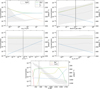 |
Fig. 12 Results for the parameter analysis. For all panels, the solid green line represents the abundance of |


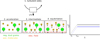 |
Fig. 13 Sketch of our electrification model. The left-hand pictures show how the process evolves overtime for the related particles, and the right-hand side shows the time evolution of the drift velocity of the related particles and the electric fields. Left: Illustration of the different phases of our electrification model. Firstly, the centrifugal force in a turbulent eddy separates the charges until an electric field builds up, which causes the molecular cations to follow the negatively charged grains. Right: Example plot of the length of timescales for acceleration and equibrilation processes shown in the left illustration. The dotted line illustrates that either the dust grains have not reached the drift velocity (black) or that the electric field is not built up yet (blue). The units are arbitrary, as this plot was only made to make the model more understandable. |
4 A simple model for turbulent charge separation
4.1 Turbulence induced electric fields
In this section, we develop a simple model to estimate the maximum electric field E that can arise when a mixture of negatively charged grains and molecular cations is shaken by turbulence. Figure 13 shows a physical sketch of the situation. We used the Richardson-Kolmogorov approach for turbulence (Richardson 1926; Kolmogorov 1941). Therefore, we assume a superposition of turbulent eddies k with various spatial scales ℓk, timescales τk, and characteristic velocities vk = ℓk/τk. In the inertial range
 (56)
(56)
is valid, where  is the energy dissipation rate toward smaller and smaller turbulent scales and ℓη and ℓL are the smallest (thermalization) and largest (driving) turbulent length scales, respectively. In the co-moving frame of a curved gas flow related to the eddy k, the dust grains are accelerated by the centrifugal force
  until an equilibrium with the frictional force Ffric in the gas is established. This problem is well known for constant gravity g (see, e.g., Woitke & Helling 2003.) After an initial acceleration timescale τacc, the grains of mass m and size a reach a constant drift velocity
  also known as the final fall speed. We took the results from Woitke and Helling for the case of a subsonic flow and large Knudsen numbers, also known as the Epstein regime. After replacing g by
  the results read:
 (57)
(57)
where τacc is the acceleration (or stopping) time, ρm is the dust material density ≈ 2 g cm−3, and  is the thermal velocity, with
  being the mean molecular weight of the gas particles.
The drift of the charged grains leads to a charge separation, which causes an electric field. How exactly this field will look is complicated and depends on the geometry and the superposition of the electric currents caused by the drifting grains in the various turbulent eddies. However, we can estimate the maximum electric field that can be generated by a single long-lived eddy by considering the case  where τΕ is the electric field buildup timescale and tk is the eddy turnover time. We assumed the electric field builds up in a coherent manner, from larger to smaller eddies, but as shown later by Eqs. (61) and (71), the main contribution comes from smaller eddies.
In this case, after the dust grains become accelerated by the eddies (Fig. 13, panel 2: acceleration), an electric field will continue to build up (Fig. 13, panel 3: intermediate) until the molecular cations in the gas follow the drifting grains because of their mobility in the E field created by the grains. We call this equilibration (Fig. 13, panel 4: equilibration), and it is characterized by a vanishing electric current:
![Mathematical equation: $ {j_{{\rm{e}}1}} = \sum\limits_j {([z_{{\rm{m}},j}^ + ] - [z_{{\rm{m}},j}^ - ])} {\mathop \upsilon \limits^^\circ _{{\rm{dr}},j}} - {n_{\rm{e}}}{\upsilon _{\rm{e}}} + \,{n_{\rm{I}}}{\upsilon _{\rm{I}}} = 0. $](/articles/aa/full_html/2023/10/aa46442-23/aa46442-23-eq120.png) (58)
(58)
As before, j is an index for the dust size bins; ![Mathematical equation: $\left[ {Z_{m,j}^ + } \right]$](/articles/aa/full_html/2023/10/aa46442-23/aa46442-23-eq121.png) ,
, ![Mathematical equation: $\left[ {Z_{m,j}^ - } \right]$](/articles/aa/full_html/2023/10/aa46442-23/aa46442-23-eq122.png) are the concentrations of the dust charge moments [charges cm−3] (see Eqs. (27) and (28)); and ne and nI are the electron and molecular cation densities [charges cm−3].
are the concentrations of the dust charge moments [charges cm−3] (see Eqs. (27) and (28)); and ne and nI are the electron and molecular cation densities [charges cm−3].
The drift velocities of the molecular cations and electrons are given by
 (59)
(59)
 (60)
(60)
where μI and μe are the mobilities of the molecular cations and free electrons, respectively, in units of cm2 s−1 V−1. The E field is measured in V cm−1. The different signs in Eqs. (59) and (60) are because of the opposite directions of the drift velocities of molecular cations and electrons in a given electric field.
If the turbulent eddy under consideration lives long enough for the drifting grains to build up the maximum, "equilibrated" electric field, it follows from Eq. (58) that
![Mathematical equation: $ E = {{\sum\nolimits_j {\left( {\left[ {Z_{{\rm{m,}}j}^ + } \right] - \left[ {Z_{{\rm{m,}}j}^ - } \right]} \right)\,} {{\mathop \upsilon \limits^^\circ }_{_{{\rm{dr}},j}}}} \over {{n_{\rm{I}}}{\mu _{\rm{I}}} + {n_{\rm{e}}}{\mu _{\rm{e}}}}}. $](/articles/aa/full_html/2023/10/aa46442-23/aa46442-23-eq125.png) (61)
(61)
From Eq. (61) we can immediately see which turbulent flows can potentially produce large E fields. Normal plasmas have ne ≈ nI » [Z+], [Z−], in which case we do not expect large turbulence-induced electric fields. Dusty plasmas, like the one we expect in region A in the disk, have [Z−] ≈ nI » ne » [Z+]. The induced electric fields in this case may be large when  is large, μΙ is small, and ne is sufficiently small to play no role, in which case nI and
 ![Mathematical equation: $\left[ {{Z^ - }} \right] = \sum\nolimits_j {\left[ {Z_{{\rm{m,}}j}^ - } \right]} $](/articles/aa/full_html/2023/10/aa46442-23/aa46442-23-eq127.png) cancel, and we find
cancel, and we find
 (62)
(62)
where ![Mathematical equation: $\left\langle {{{\mathop \upsilon \limits^^\circ }_{{\rm{dr}}}}} \right\rangle = \sum\nolimits_j {\left[ {Z_{{\rm{m,}}j}^ - } \right]{\upsilon _{{\rm{dr,}}j}}/\sum\nolimits_j {\left[ {Z_{{\rm{m,}}j}^ - } \right]} } $](/articles/aa/full_html/2023/10/aa46442-23/aa46442-23-eq129.png) is the charge-mean grain drift velocity. There is another case when [Z−] ≈ [Z+] » nI, ne. In that case, which we call “region X” (not found in our present disk models), large E fields might be produced when many small grains are strongly charged negatively and many large grains are strongly charged positively, or vice versa, such that the nominator in Eq. (61) remains large despite charge neutrality in an isolating gas with few charged gas particles. We note that tribolelectric charging, which is not included in our current disk models, might be able to turn parts of region A into a region X.
is the charge-mean grain drift velocity. There is another case when [Z−] ≈ [Z+] » nI, ne. In that case, which we call “region X” (not found in our present disk models), large E fields might be produced when many small grains are strongly charged negatively and many large grains are strongly charged positively, or vice versa, such that the nominator in Eq. (61) remains large despite charge neutrality in an isolating gas with few charged gas particles. We note that tribolelectric charging, which is not included in our current disk models, might be able to turn parts of region A into a region X.
We mention that at this point, there are alternative approaches to how we consider ion and electron mobilities. In Okuzumi & Inutsuka (2015), they present analytic expressions for ion and electron drift velocities in an H2 gas.
In order to estimate the duration of the equilibration phase in Fig. 13, henceforth called the E field buildup timescale τΕ, we considered the travel time of the grains
 (63)
(63)
where d is the charge separation distance, that is, the distance between the moving grains and the moving molecular ions causing the electric field E. To estimate that distance, we considered the most simple geometry of a parallel plate capacitor (with equations in SI units):
 (64)
(64)
![Mathematical equation: $ {Q_{{\rm{SI}}}} = e\,{\left[ {{Z^ - }} \right]_{{\rm{SI}}}}\,A\,{d_{{\rm{SI}}}} $](/articles/aa/full_html/2023/10/aa46442-23/aa46442-23-eq132.png) (65)
(65)
![Mathematical equation: $ \Rightarrow {d_{{\rm{SI}}}} = {{{_0}{E_{{\rm{SI}}}}} \over {e\,{{[{Z^ - }]}_{{\rm{SI}}}}}}, $](/articles/aa/full_html/2023/10/aa46442-23/aa46442-23-eq133.png) (66)
(66)
where ϵ0 is the electric vacuum permittivity and e is the electron charge in SI units; ESI = 102 E is the maximum electric field in [Vm−1]; A is a horizontal area [m2] that cancels; [Z−]SI = 106 [Z−] is the concentration of negative charges on dust grains in ![Mathematical equation: $\left[ {{{\rm{m}}^{ - 3}}} \right];\,\,{d_{{\rm{SI}}}} = {10^{ - 2}}$](/articles/aa/full_html/2023/10/aa46442-23/aa46442-23-eq134.png) d is the charge separation distance in [m]; and QSI is the total negative charge on the grains in volume dSI × A in [C]. Equations (57), (63), and (66) provide an estimate for the time required to clear a volume d × A from dust grains of size a by centrifugal forces in a turbulent eddy k, which results in an overpopulation of negative charges at the lower boundary and missing negative charges at the upper boundary, which together build up the maximum electric field.
d is the charge separation distance in [m]; and QSI is the total negative charge on the grains in volume dSI × A in [C]. Equations (57), (63), and (66) provide an estimate for the time required to clear a volume d × A from dust grains of size a by centrifugal forces in a turbulent eddy k, which results in an overpopulation of negative charges at the lower boundary and missing negative charges at the upper boundary, which together build up the maximum electric field.
Thus, we have three different timescales to consider that may depend on the considered particle size a and the selected turbulent eddy k. In most cases, we found
 (67)
(67)
to be valid, that is, the turbulent eddy lives long enough to allow the grains to accelerate quickly and then drift for long enough distances to cause the maximum electric field. If relation (67) does not hold, Eq. (61) is not valid.
For the ion mobility μI we considered the NH4+ cation, as we found this molecule to be the most abundant gas charge carrier in region A. Abedi et al. (2014) presented measurements for the mobility of  in a N2 gas at standard pressure and temperature, P0 = 760 Torr and T0 = 273 K, which we denote by
  As the most abundant species in the disks is H2, we needed to adjust this value. This was done by multiplying with the ratio of the reduced masses of N2 and H2 with NH4+, denoted with
  and
and  , respectively, and scaling with the gas particle density (see Eq. (4) in Abedi et al. 2014):
 (68)
(68)
The electron mobility μe was calculated from the drift velocity measurements for electrons of Ryzko (1965) and calculated as
 (69)
(69)
with υdr,e measured in dry air to be
![Mathematical equation: $ {\upsilon _{{\rm{dr}},{\rm{e}}}} = 256 \times {10^3}{E \over {{E_0}}}{{{P_0}} \over P}{T \over {{T_0}}}[{\rm{cm}}\,{{\rm{s}}^{ - 1}}], $](/articles/aa/full_html/2023/10/aa46442-23/aa46442-23-eq142.png) (70)
(70)
where P0 and T0 are the same as for the ion mobility and E0 = 75 Vcm−1. This formula results in an electron mobility that is about a factor of 200 larger than the mobility of NH4 +. As the original measurements were done in dry air, we would have to adjust our mobility calculations in the same way we did for ion mobility, but due to only minor differences in reduced masses when considering the electron mass, we omitted making a similar correction.
According to our charge separation model, the electric fields that can potentially be caused by turbulence are proportional to the centrifugal accelerations  that the turbulent eddies can provide. Following Eq. (56), we found
 (71)
(71)
that is, the smallest eddies cause the largest centrifugal forces. We therefore considered the Kolmogorov timescale tη, that is, the turnover timescale of the smallest eddy in the inertial subrange. Following Ormel & Cuzzi (2007), we determined τη by
 (72)
(72)
where τL is the turnover timescale of the largest eddy in our system and ℛe is the Reynolds number defined by
 (73)
(73)
where υL is the velocity of the largest eddy, ℓL is its size, and vkin is the kinematic viscosity. The kinematic viscosity is from Woitke & Helling (2003). Using their formula for the dynamic viscosity, we got  . For the size and velocity of the largest eddy, we assumed
  and
and  (see Ormel et al. 2007), where Hp is the pressure scale height, which is set in our simulations as
 (74)
(74)
The resulting size of the smallest turbulent eddy ℓη is considerably larger than the gas mean free path  by about four orders of magnitude, but it is also much smaller in scale height by about eight orders of magnitude.
Since we wanted to maximize the effect of the turbulence, we had to choose the τk that maximizes the centrifugal acceleration. Additionally we had to choose a time that allows the electrical fields to develop. Therefore, we followed the principle that we choose the shortest time that is still long enough for the fields to develop. This is illustrated by Fig. 14. Following this principle of smallest time that still lets the fields develop, we can see that in most cases we can choose τk = τη. In cases with larger grains, a > 10−1cm, we would choose τk = τacc to ensure the grains have enough time to reach their drift velocity  .
.
With these results, we could then calculate what electric fields would result from the interaction of our dust and gas mixture in a turbulent eddy and answer the question of whether lightning could emerge with this mixture already. Nonetheless, we still had to consider how large these electric fields could be. For lightning to emerge in any medium, the electric fields generated have to be large enough for an electron cascade to occur. We followed the description and Eq. (56) from Muranushi & Tomiyasu (2009). With this we were able to define a critical electric field, Ecrit, that is the electric field at which an electron cascade can occur because the electrons are accelerated enough to ionize the neutral components of the gas:
 (75)
(75)
Here, ∆W is the ionization energy required to ionize the neutral components, e is the coulomb constant, and λ is the mean free path. For ∆W, we took the ionization energy of H2 with 15.4 eV. To determine, λ we followed Eq. (10) of Woitke & Helling (2003).
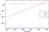 |
Fig. 14 Comparison of the different timescales considered in our turbulence implementation. |
4.2 Electric field magnitudes
In this section, we discuss our investigation of the magnitude of the previously discussed turbulence-induced electric fields. We took the data from our simulations that we made for investigating the dust charge behavior from Sect. 3.6 to perform this investigation. The resulting electric fields are shown in Fig. 15.
Minimal dust size. We found that if one changes the minimal dust size, one first sees an increase in electric field strength due to the increase in dust size and in drift velocity and therefore in electric field strength as well. However, with a minimum dust grain size of more than 0.5μm, a decrease in electric field strength occurs. This is due to the fact that larger dust grains are less abundant in our model. Regarding the way we set up the simulations, only very large dust grains were considered, and therefore the dust abundance drops. According to Eq. (61), this of course has a negative impact on the total electric field strength.
Dust-to-gas ratio. For increasing dust-to-gas ratios, we observed a steady increase in electric field strength until a saturation took place at our standard value of 10−2. The reason for the low electric field values at lower dust-to-gas ratios is again the fact that fewer dust grains can contribute positively toward the creation of electric fields.
Cosmic rays. The influence of cosmic rays on the electric fields is not very surprising given their strong link to electron abundance. High cosmic ray ionization rates result in high electron abundances and therefore low electric fields, due to the attenuating effect electrons have on the buildup of electric fields. The reverse is true for low cosmic ray ionization rates, however, and this effect stagnates at around 10−19[s−1].
Gas density. One could expect that the gas density has a similar effect on the electric fields as the cosmic ray ionization rate, but this does not fully hold. While the general trend is the same, that is, where high gas densities reduce the electron abundance due to the larger shielding, there are more effects that must be mentioned. Compared to the other tests where the critical field is kept constant, we found that the critical field rises with increasing gas densities. This is also the case with higher gas density: the mean free path increases, which increases the required energy for an electron avalanche to occur. We also found that for gas densities lower than our standard value, one can observe an enhancing factor for the electric fields. This is because of the reduced drag on the dust grains in lower gas densities. This in turn increases the drift velocities of the dust grains and can therefore enhance the charge separation and the electric fields.
However, one general trend holds true for all of the studied combination of parameters discussed above, namely, the resulting electric fields are several orders of magnitude smaller than the required critical field. Nonetheless, we can still use this study to state which conditions are best for lightning to emerge. We therefore state that the most likely parameter conditions for lightning to emerge in a protoplanetary disk include having large and abundant dust grains in an area with a low cosmic ray ionization rate and low gas density.
Dust temperature. To calculate the electric field strength for the simulations where we varied the dust temperature, we had to adjust our calculations of the electric field, as the most abundant positive ion for certain temperatures is Na+ and not NH4+. We adjusted Eq. (61) to account for the concentration of Na+,  , and their mobility
  :
:
![Mathematical equation: $ E = {{\sum\nolimits_j {\left( {\left[ {{\rm{Z}}_{{\rm{m,}}j}^ + } \right] - \left[ {{\rm{Z}}_{{\rm{m,}}j}^ - } \right]} \right)\,} {\upsilon _{{\rm{dr}},j}}} \over {({n_{\rm{I}}}{\mu _{\rm{I}}} + {n_{{\rm{N}}{{\rm{a}}^ + }}}{\mu _{{\rm{N}}{{\rm{a}}^ + }}}) + {n_{\rm{e}}}{\mu _{\rm{e}}}}}. $](/articles/aa/full_html/2023/10/aa46442-23/aa46442-23-eq156.png) (76)
(76)
We calculated the mobility of Na+ in a manner similar to the  :
:
 (77)
(77)
We took 17.5 [cm2 V−1 s−1] for  , according to Loeb (1931), who measured the mobility of Na+ in H2. We chose the two normalization factors [P0] and [T0] to be the same as for our
  calculations.
With these additional calculations in place, we could analyze the behavior of the electrical field at different temperatures. We note that in our analysis, we omitted the first point at 100 K, as including it would have required taking  into account with its mobility. We identified three different trends in the electric field curve. First, we identified a steady increase in electric field strength from 200 K up to 1300 K. This can be explained by the steady increase we observed in the concentration of negatively charged dust grains and the
  relative to the electron concentration.
From 1400 K to 1600 K, we first observed a drop by nearly a factor of two and then a plateau. This can be explained by the Na+ ions having become the most relevant positive species. As their mobility is larger by nearly a factor of ten, it is harder for the dust grains to obtain high amounts of separation compared to the case with  .
.
Lastly, we observed a continuous drop in electric field strength until 1800 K. This can be explained by the electron concentration becoming relevant again. As shown in Sect. 3.6, the dominant reaction creating Na+ also creates free electrons. Due to the very high mobility of the free electrons, they can strongly inhibit the buildup of the electrical field. Their mobility is about two orders of magnitude higher than the ones we found for our positive molecules. Hence, their effect can already be seen when their concentration is still at only about 1% of the negative dust grains and positive molecules.
In conclusion, the picture that presents itself when we modify the dust temperature is more complicated than for our other examples. In isolation, where we would just observe a system of dust grains and one other positive species, one could conclude that higher temperatures show a positive impact on electrical field strength. But as shown in our example, this is an oversimplification, and one should always consider the other effects an increase in temperature can have.
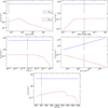 |
Fig. 15 Electric fields resulting from turbulence induced eddies for the different parameter variations shown in Sect. 3.6. The red line represents said electric fields, and the blue line shows the critical electric field as from Eq. (75). The solid black lines again represent the conditions from our standard simulation. We note that for the sake of visibility, the y-axis is interrupted, as the differences between the critical fields and the turbulence induced fields are quite large. |
5 Discussion of the charge balance in region A under consideration of ion attachment
In this section, we discuss the charge balance in a case where a physical attachment between NH4+ and negative dust grains would be possible. Although the dissociative recombination reaction Z− + NH4+ → Z + NH3 + H is energetically forbidden, the NH4+ ion could be trapped in the electrostatic potential of a strongly negatively charged grain, either after a collision with its surface or after an inelastic collision with a gas particle close to the surface. This could occur when the electrostatic potential  is much larger than the molecule’s thermal energy kT. At a temperature of 100 K, this corresponds to a negative dust charge of |q|/a ≫ 6 μm−1. In such cases, the NH4+ molecule would be expected to stick to the surface or to stay in close vicinity of the surface.
Such an attachment reaction could be formally written as
 (78)
(78)
The compound  would hold both the negative charges of the accumulated electrons and the positive charges of the accumulated molecular ions and would therefore be considerably less negative in the far field due to shielding by the NH4+.
We assumed that the overall effects of such a mechanism would not significantly change the charge balance we found in region A but could result in an increase of the non-shielded negative dust grain charge q/a. This would introduce a new destruction path for NH4+ with such a reaction, therefore decreasing the amount of NH4+ in the gas. This could increase the electron concentration in the charge balance, but the  compound is less negatively charged than a dust grain Z−, and it would result in more free electrons attaching to the compound compared to a dust grain. This process would increase the non-shielded grain charge q/a until the shielded negative grain charge becomes similar to the q/a calculated in this paper. In conclusion, such a process would act as a sink of both
  and free electrons, while it would increase the non-shielded negative q/a.
However, in order to implement these effects into this work, one would need more data about the microphysical details of these processes, as such a reaction would not only need to be considered for NH4+ but also for every other positive molecule with a proton affinity higher than about 8 eV (Table 2), and one would need a kinetic formulation of the back reactions. Therefore, inclusion of this mechanism goes beyond the scope of this paper, but it could be the subject of a follow-up study.
6 Summary and conclusion
We identified six different regions in our disk simulations with significantly different charging behaviors of dust and gas. The three upper regions (D, E, and F) are all photon dominated, the dust grains are positively charged, and the charge balance of the grains is characterized by an equilibrium between photoionization and electron attachment. The free electrons are generated by photoionization, leading to H+ in region F, C+ in region E, and S+ in region D.
In the lower disk regions (A, B, and C), we found a more complex picture with negatively charged grains. In these regions, the electron concentration is significantly lower due to the almost complete shielding from UV and X-rays. This leaves cosmic ray ionization of molecular hydrogen as the most significant mechanism for electron production. The grain charge balance is characterized by an equilibrium between electron attachment and charge exchange reactions with molecular cations.
Region C is metal poor due to ice formation, and H3+ is the most abundant molecular cation. Region B has a very complex hydrocarbon chemistry, as nitrogen and oxygen are already frozen out, but carbon is not. The most abundant molecular cation was found to be C3H3+, due to its large proton affinity. We found that negatively charged dust grains Z− become more abundant than free electrons inward of about r = 3 au in our standard T Tauri disk model.
In region A, we found very low concentrations of free electrons between about 10−13 and 10−18. The low electron concentration is because of the free electrons attaching themselves very quickly to dust grains at the high gas densities in region A. A charge balance becomes established between negatively charged dust grains Z− and positively charged molecular ions, whereas the free electrons do not play an important role in the charge balance in region A. We found NH4+ to be the most abundant molecular cation by far, due to its very high proton affinity, and since region A is too warm for NH3 ice to form, NH4+ is available.
Additionally, we found that the charge of a dust grain q depends linearly on its size a in almost all cases and in all disk regions (i.e., q/a = const). In disk region A, we found q/a ≈ −350 charges per micrometer to be a typical value. This linear dependence is because of the electric grain potential oc q/a, which enters the various photo-electron attachment and charge exchange rates.
We studied how the quantities characterizing the charging behavior of gas and dust depend on certain gas, dust, and cosmic ray properties in region A. These properties include the electron density ne, the molecular cation density  , the density of negative charges on grains Z−, and q/a. In particular, we found that the electron concentration depends linearly on the cosmic ray ionization rate in region A, while this rate has no effect on Z−and
  . We found that at a cosmic ray ionization rate as low as 10−22 s−1, the electron concentrations can drop to < 10−19. The gas density has the opposite effect, as lower gas densities cause higher electron concentrations.
The minimum dust size and the dust-to-gas ratio also have pronounced effects on ne,  , and Z−. In particular, higher dust/gas ratios cause lower electron concentrations, an effect that seems essential to understanding ring formation in early disks via disk instabilities (see Regaly et al. 2023).
Higher gas temperatures more strongly favor negatively charged grains, as the higher thermal velocities of the free electrons allow them to still collide with the grains, even if they are already strongly charged negatively. However, at temperatures roughly over 1300 K, thermal ionization of Na leads to a sudden increase of the electron concentration.
We find region A to be the most likely site for lightning to occur in disks. This is because the electron concentration in region A is so low that the gas effectively becomes an insulator, and the dynamics of the charged grains can cause an electrification.
We developed a simple model for the electrification due to turbulence in which a charge separation between the positive NH4+ molecules and the negative dust grains occurs due to the centrifugal force in turbulent eddies. While this mechanism does not generate electric fields large enough to overcome the critical electric field for an electron cascade to occur in our standard T Tauri disk model, we still used it to explore areas in the disk that present the best conditions for lightning to emerge. According to this electrification model, we favor low cosmic ray ionization rates, high dust-to-gas ratios, large dust grains, and small gas densities. The model also favors warm gas temperatures, but no higher than about 1300 K, where the thermal ionization of Na inhibits the buildup of electric fields by creating too many charged gas particles that enhance the gas conductivity.
So far, we have not yet included triboelectric charging rates in our disk models. This effect, which generates negatively charged small grains and positively charged large grains by dust-dust collisions, could lead to a situation where both Z+ and Z− are larger by orders of magnitude compared to our current results, whereas the concentrations of free electrons and molecular cations can remain very low. In that case (i.e., region X), our turbulent electrification model (Eq. (61)) predicts much larger electric fields that could potentially reach the critical E field for electron cascade (i.e., lightning).
In preliminary studies, we noticed that the grain charge chemistry is very sensitive to the heat of formation of charged dust grains  (Zq) connected to the work function and the band gap. As alluded to at the end of Sect. 2.4, the underlying physics here are complicated, and the value is rather uncertain, depending on the material mixture, surface properties, and ice coating. We would like to investigate this question further in an upcoming study, where we would test different chemical potentials and show the effects this value might have on the midplane chemistry and the potential emergence of lightning.
Acknowledgements
T.B., P.W., and U.G.J. acknowledge funding from the European Union H2020-MSCA-ITN-2019 under Grant Agreement no. 860470 (CHAMELEON). U.G.J. further acknowledges funding from the Novo Nordisk Foundation Interdisciplinary Synergy Programme grant no. NNF19OC0057374.
Appendix A Additional table
Glossary of symbols with units used in this paper.
Appendix B On the impact of automatically generated charge exchange and protonation reactions
The three different models we considered when testing the influence of automatically generated reactions.
In this section, we investigate the effect that automatically generated charge exchange, protonation, and endothermic reactions can have on our model. For this, we incorporated three different models (Tab. B.1): one where we do not allow exchange, protonation, or endothermic reactions to be generated and only use the network as provided, from now on called “noEX”; one where we allow charge exchange reactions to be generated, which is the case for our standard case discussed before; and one where we allow charge exchange, protonation, and endothermic reactions tobegenerated, fromnow oncalled”EX.”Wenotethatfor endothermicreactions, wesetthebarrieroftheactivationenergy for the reactions to be at 5000 Kkb, which equals to 0.431 eV.
To illustrate the differences between the three models, we wanted to show a list of the different reactions considered for the different setups. However, such a list would consider thousands of reactions since our noEX setup consists of 5530 reactions, the standard setup of 7009, and the EX of 8672, and we would have to show the differences with example reactions, meaning reactions of a specific type not considered by a certain setup. Therefore, we have chosen instead to present a curated list of reactions that show what kind of reactions are additionally considered for the different setups (Tab. B.2).
Appendix B.1: noEx model
For the noEx model in region A, we found that, firstly, the whole region A starts a bit farther in, due to  dipping at a later point. Secondly, we found that C4H+ is more abundant much farther in. For region B, we again found the trend that the region emerges more inward than in our standard case. Overall, we found the chemistry to be very comparable. We however found that the species H2S+ and H2CS+ are more abundant and overcome our set threshold, while SiOH+ and H3CO+ do not overcome this threshold and are therefore no longer abundant. For region C and outward, we found no notable differences.
Appendix B.2: EX model
For region A, we mainly found that compared to our standard model, Na+ becomes the second most abundant positive charge carrier and replaces NaH2+. In addition, we found that Fe+ is no longer abundant enough to meet our set threshold. However, we found protonated methanol  to be abundant in the EX model. For region B, we found a much less complex chemistry. In particular, C4H+ and HCNH+, which are abundant in our standard model, do not show up anymore. We only found the sulfur bearing species, which are also abundant in the standard model, dominate as the second and third most abundant cations after
  . For region C, we again found no significant differences.
Example reactions present in the different models.
Appendix C Solving the chemical rate network with dust charge moments
The charge and size distribution of the dust grains are represented in our chemical models by three charge moments,  , Zm,j, and
  , in each dust size bin, using a small number of dust size bins j є {1, …, J}. In Sect. 2.8, we introduced the effective chemical rates for these moments for photoionization, electron attachment, and charge exchange reactions, which properly describe the overall effect of all grains on the gas and ice chemistry. On one side, the charge distribution function fj(q) must be known to calculate the effective rate coefficients. However, on the other side, as explained in Sect. 2.7, the determination of fj(q) requires knowing the photon flux and the concentrations of all chemical species, including electrons and molecular anions and cations.
Our formulation with dust charge moments and effective rates still conforms with the basic shape of a coupled system of first-order ODE system,
 (C.1)
(C.1)
which enables us to use numerical ODE solvers to advance the chemistry. The term ni is the particle density of chemical species i, n = {n1, …,nI} is the solution vector, Pi and Li are the total production and destruction rates, Fi represents the components ofthe right-hand side (RHS) vector, and I is the numberofchemical species that include 3 × J dust moments. From n, we could in principle update fj(q) in each call of the RHS vector, then update the effective rate coefficients, and calculate all Fi. However, this would result in an extremely slow computational method because the calculation of fj(q) requires the computation of tens of thousands of rates for all individual charging states. In addition, we would need implicit solvers, which require the Jacobian derivative ∂Fi/∂nj, that is, for each integration step one would need to carry out the determination of fj(q) a couple of 100 times. Normally in astrochemistry, one can calculate the rate coefficients only once, prior to calling the ODE solver, because the rate coefficients do not depend on the particle densities, and then compute Fi and ∂Fi/∂nj from these rate coefficients in very efficient, quick ways. In contrast, according to our formulation of the problem, the rate coefficients here depend on the particle densities in complicated ways.
We figured that there is a much more efficient way to solve our chemical equations by means of an iterative approach. To obtain a time-independent solution of our chemical equations, as used in this paper, we followed the following algorithm:
(1) Provide an initial guess of the particle densities n based on the results obtained for the previously solved grid point.
(2) Compute fj(q) from n.
(3) Compute all rate coefficients, including the effective rate coefficients, from fj(q).
(4) Solve F(nnew) = 0 for given rate coefficients to obtain the new solution vector nnew.
(5) Compute the relative changes of electron density ne and mean grain charges <qj> in all size bins j between iterations.
(6) If these relative changes are <10−5 and <10−2, respectively, then take nnew as solution and stop the iteration.
(7) Provide a better guess for n and jump back to (2).
For step (7), we applied the following strategy. Each iteration was assigned a quality defined as Qnew = - ne. At first instance, we took n ← nnew as the improved guess in step (7), that is, we performed a Λ iteration. In all subsequent calls, we used the previous and current electron densities and Q values to provide a better guess of the solution vector,
 (C.2)
(C.2)
 (C.3)
(C.3)
by determining the value for X that nullifies Q in case Q is a linear function of ne, that is, we performed a Newton step. Precisely speaking, we put  where we found
  from the two previous iterations to determine the next improved guess of the electron density
  related to
 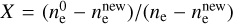 . If the magnitude of the new quality Qnew was much smaller than the magnitude of the old quality Q, X was close to zero, and we essentially performed another Λ iteration. The reader may verify that the resulting electron density according Eq. (C.3) is indeed
  . This numerical method typically converges within a couple of iterations. In a few cases, however, the method started to oscillate. We therefore monitored the Q values and saved the n vectors that were encountered during the iteration. Once we found the negative and positive entries for Q, we bracketed the solution and used the two iterations that produced the smallest positive and largest negative Q values to provide a better next guess for n in step (7).
In case we required a time-dependent solution of Eq. (C.1), not performed in this paper, we used a different strategy. The problem in this case is that with constant rate coefficients, the solution may start to alternate between two charging states with every time step taken. For example, highly negatively charged grains do not take any more electrons (i.e., the km,j,e become small), which means that during the next time step, the grains charge up less negatively, and so on. Our solution here was to monitor the dependencies of the effective rate coefficients kr on electron density ne and use the correction power law
 (C.4)
(C.4)
whenever the ODE solver required the RHS or the Jacobian. The term  is a reference electron density from which
  was calculated, and ne is the actual electron density occurring during the integration. The term pr is a rate coefficient correction power law index. The initial conditions were
  , and pr = 0.
The whole time-dependent approach can be summarized in eight steps:
(1) Compute fj(q) from n and rate coefficients  from fj(q).
(2) Advance the chemistry for time step ∆t from n with rate coefficients according to Eq. (C.4), resulting in nnew(t + ∆t).
(3) Compute new fj(q) and new rate coefficients  from nnew.
(4) Update the rate coefficient correction indices as pr =  .
.
(5) Assess the uncertainty ∆n based on the difference between k and knew and ∆t.
(6) Limit the increase of the next time step ∆t when large relative uncertainties ∆ni/ni are found.
(7) If t + ∆t reaches the requested total integration time, take nnew as the solution and stop the iteration.
(8) Update  and jump back to (2).
This algorithm can slow down the computation of a t-dependent solution when strong oscillations would occur, resulting in large ∆ni where smaller time steps are indeed required. However, the algorithm manages to sufficiently damp these oscillations and quickly re-increases the time step once the conditions have changed and the oscillations disappear.
Appendix D Dissociative molecular ion attachment reactions
Consider a reaction between dust grains and NH4+ molecules, in which the NH4+ molecule dissociates,
 (D.1)
(D.1)
where z−(q−1) is a dust grain that is less negatively charged than Z−q by a factor of one. The reaction enthalpy, which tells us whether a reaction is exothermic or endotherm, is given by
 (D.2)
(D.2)
where Hf is the heat of formation of a substance from a chemical standard state, which we set here as purely atomic in the absence of electric fields. For neutral molecules, we used the atomization energies  derived from the standard enthalpies at 0K from UMIST (Woodall et al. 2007), but for Hf (NH4+), we needed to take into account the electric potential in the presence of the electric field of the dust grain at its surface
 (D.3)
(D.3)
 (D.4)
(D.4)
 (D.5)
(D.5)
The heat of formation of a negatively charged dust grains is
 (D.6)
(D.6)
where Hf (atoms → Z0) is the heat of formation of a dust grain from the atoms it is composed of. The term Hf (Z−(i−1) → Z−i) describes the energy liberated when moving a single electron from infinity to the grain’s surface (takes energy) and then attaching it to the surface (liberates energy E0)
 (D.7)
(D.7)
Using the Gaussian sum formula, the total formation enthalpy of a negatively charged grain is hence
 (D.8)
(D.8)
From Eq. (12), we could identify the constant E0 = W0 − Ebg, where W0 is the work function and Ebg the band gap, and we assumed both to be independent of q.
The reaction enthalpy according to Eq. (D.2) is then given by
 (D.9)
(D.9)
where the proton affinity is  , and
, and  is the ionization energy of hydrogen. Since the term e2/a is negligible even for grains as small as 0.1 μm, Eq. (D.9) allowed us to state that a dissociative attachment reaction is exothermal when the work function minus the band gap plus the proton affinity of the respective molecule is smaller than 13.6 eV, independent of q.
There is, however, a small correction term of order e2/a that complicates things. In our derivation, this term arises from the removal of one electron and one positive molecular ion from the electric field at the grain surface by the reaction, and this term is size dependent. Similar correction terms appear in Eqs. (12) and (13). In the current code version, we used E0 = 5.89 eV, as explained in more detail at the end of Section 2.4.
References
- Abedi, A., Sattar, L., Gharibi, M., & Viehland, L. A. 2014, Int. J. Mass Spectrom., 370, 101 [NASA ADS] [CrossRef] [Google Scholar]
- Akimkin, V. V., Ivlev, A. V., & Caselli, P. 2020, ApJ, 889, 64 [NASA ADS] [CrossRef] [Google Scholar]
- Aresu, G. 2012, PhD thesis, University of Groningen, The Netherlands [Google Scholar]
- Bai, X.-N. 2011, ApJ, 739, 50 [CrossRef] [Google Scholar]
- Bai, X.-N., & Stone, J. M. 2011, ApJ, 736, 144 [Google Scholar]
- Baines, K. H., Delitsky, M. L., Momary, T. W., et al. 2009, Planet. Space Sci., 57, 1650 [NASA ADS] [CrossRef] [Google Scholar]
- Baker, B., Baker, M. B., Jayaratne, E. R., Latham, J., & Saunders, C. P. R. 1987, Q. J. Roy. Meteorol. Soc., 113, 1193 [NASA ADS] [CrossRef] [Google Scholar]
- Brook, M., Moore, C. B., & Sigurgeirsson, T. 1974, J. Geophys. Res., 79, 472 [NASA ADS] [CrossRef] [Google Scholar]
- Bruning, E. C., Rust, W. D., Schuur, T. J., et al. 2007, Monthly Weather Rev., 135, 2525 [CrossRef] [Google Scholar]
- Cleeves, L. I., Adams, F. C., & Bergin, E. A. 2013, ApJ, 772, 5 [Google Scholar]
- Cuzzi, J. N., Hogan, R. C., Paque, J. M., & Dobrovolskis, A. R. 2001, ApJ, 546, 496 [NASA ADS] [CrossRef] [Google Scholar]
- D’Angelo, M., Cazaux, S., Kamp, I., Thi, W. F., & Woitke, P. 2019, A & A, 622, A208 [CrossRef] [EDP Sciences] [Google Scholar]
- Dash, J. G., Mason, B. L., & Wettlaufer, J. S. 2001, J. Geophys. Res., 106, 20,395 [Google Scholar]
- Delitsky, M. L., & Baines, K. H. 2015, Planet. Space Sci., 113, 184 [CrossRef] [Google Scholar]
- Desch, S. J., & Cuzzi, J. N. 2000, Icarus, 143, 87 [Google Scholar]
- Drazkowska, J., Bitsch, B., Lambrechts, M., et al. 2023, ASP Conf. Ser., 534, 717 [NASA ADS] [Google Scholar]
- Dubrulle, B., Morfill, G., & Sterzik, M. 1995, Icarus, 114, 237 [Google Scholar]
- Dullemond, C. P., & Dominik, C. 2004, A & A, 421, 1075 [NASA ADS] [CrossRef] [EDP Sciences] [Google Scholar]
- Dullemond, C. P., & Penzlin, A. B. T. 2018, A & A, 609, A50 [NASA ADS] [CrossRef] [EDP Sciences] [Google Scholar]
- Dyudina, U. A., Ingersoll, A. P., Ewald, S. P., et al. 2010, Geophys. Res. Lett., 37, L09205 [Google Scholar]
- Feuerbacher, B., & Fitton, B. 1972, J. Appl. Phys., 43, 1563 [NASA ADS] [CrossRef] [Google Scholar]
- Forward, K. M., Lacks, D. J., & Sankaran, R. M. 2009, Phys. Rev. Lett., 102, 028001 [NASA ADS] [CrossRef] [Google Scholar]
- Gaudin, D., Cimarelli, C., Becker, V., & Knüver, M. 2018, EGU General Assembly Conference Abstracts, 12793 [Google Scholar]
- Gurevich, A. V., & Zybin, K. P. 2005, Phys. Today, 58, 37 [NASA ADS] [CrossRef] [Google Scholar]
- Helling, C., & Rimmer, P. B. 2019, Philos. Trans. Roy. Soc. Lond. A, 377, 20180398 [NASA ADS] [Google Scholar]
- Helling, C., Jardine, M., & Mokler, F. 2011, ApJ, 737, 38 [Google Scholar]
- Helling, C., Harrison, R. G., Honary, F., et al. 2016, Surv. Geophys., 37, 705 [NASA ADS] [CrossRef] [Google Scholar]
- Hill, R. D., Rinker, R. G., & Wilson, H. D. 1980, J. Atmos. Sci., 37, 179 [NASA ADS] [CrossRef] [Google Scholar]
- Hodosán, G., Helling, C., Asensio-Torres, R., Vorgul, I., & Rimmer, P. B. 2016, MNRAS, 461, 3927 [Google Scholar]
- Houghton, I. M. P., Aplin, K. L., & Nicoll, K. A. 2013, Phys. Rev. Lett., 111, 118501 [NASA ADS] [CrossRef] [Google Scholar]
- Inutsuka, S.-I. & Sano, T. 2005, ApJ, 628, L155 [NASA ADS] [CrossRef] [Google Scholar]
- Ivlev, A. V., Akimkin, V. V., & Caselli, P. 2016, ApJ, 833, 92 [NASA ADS] [CrossRef] [Google Scholar]
- Jayaratne, E. R., Saunders, C. P. R., & Hallett, J. 1983, Q. J. Roy. Meteorol. Soc., 109, 609 [NASA ADS] [Google Scholar]
- Johansen, A., & Okuzumi, S. 2017, in LPI Contributions, 1963, Chondrules and the Protoplanetary Disk, ed. LPI Editorial Board, 2012 [Google Scholar]
- Jungmann, F., & Wurm, G. 2021, A & A, 650, A77 [NASA ADS] [CrossRef] [EDP Sciences] [Google Scholar]
- Kamp, I., Thi, W. F., Woitke, P., et al. 2017, A & A, 607, A41 [NASA ADS] [CrossRef] [EDP Sciences] [Google Scholar]
- Kolmogorov, A. 1941, Akad. Nauk SSSR Dokl., 30, 301 [Google Scholar]
- Kopnin, S. I., Kosarev, I. N., Popel, S. I., & Yu, M. Y. 2004, Planet. Space Sci., 52, 1187 [NASA ADS] [CrossRef] [Google Scholar]
- Lacks, D. J., & Levandovsky, A. 2007, J. Electrostatics, 65, 107 [CrossRef] [Google Scholar]
- Lesur, G., Flock, M., Ercolano, B., et al. 2023, in ASP Conf. Ser., 534, Astronomical Society of the Pacific Conference Series, eds. S. Inutsuka, Y. Aikawa, T. Muto, K. Tomida, & M. Tamura, 465 [Google Scholar]
- Leung, C. M., Herbst, E., & Huebner, W. F. 1984, ApJS, 56, 231 [CrossRef] [Google Scholar]
- Linstrom, P., & Mallard, W. 2022, NIST Chemistry Webbook: NIST StandardReference Database Number 69 (NIST), google-Books-ID: dxM3ngAACAAJ [Google Scholar]
- Loeb, L. B. 1931, Phys. Rev., 38, 549 [NASA ADS] [CrossRef] [Google Scholar]
- McElroy, D., Walsh, C., Markwick, A. J., et al. 2013, A & A, 550, A36 [NASA ADS] [CrossRef] [EDP Sciences] [Google Scholar]
- Méndez Harper, J., Helling, C., & Dufek, J. 2018, ApJ, 867, 123 [NASA ADS] [CrossRef] [Google Scholar]
- Millar, T. J., Farquhar, P. R. A., & Willacy, K. 1997, A & AS, 121, 139 [NASA ADS] [Google Scholar]
- Muranushi, T. 2010, MNRAS, 401, 2641 [Google Scholar]
- Muranushi, T., & Tomiyasu, T. 2009, in AIP Conf. Ser., 1158, Exoplanets and Disks: Their Formation and Diversity, eds. T. Usuda, M. Tamura, & M. Ishii, 145 [CrossRef] [Google Scholar]
- Murray, L. T., Logan, J. A., & Jacob, D. J. 2013, J. Geophys. Res. (Atmos.), 118, 11,468 [CrossRef] [Google Scholar]
- Navarro-González, R., McKay, C. P., & Mvondo, D. N. 2001, Nature, 412, 61 [CrossRef] [Google Scholar]
- Noxon, J. F. 1976, Geophys. Res. Lett., 3, 463 [NASA ADS] [CrossRef] [Google Scholar]
- Okuzumi, S. 2009, ApJ, 698, 1122 [Google Scholar]
- Okuzumi, S., & Inutsuka, S.-I. 2015, ApJ, 800, 47 [NASA ADS] [CrossRef] [Google Scholar]
- Okuzumi, S., Tanaka, H., Takeuchi, T., & Sakagami, M.-A. 2011, ApJ, 731, 95 [NASA ADS] [CrossRef] [Google Scholar]
- Okuzumi, S., Mori, S., & Inutsuka, S.-I. 2019, ApJ, 878, 133 [NASA ADS] [CrossRef] [Google Scholar]
- Ormel, C. W., & Cuzzi, J. N. 2007, A & A, 466, 413 [NASA ADS] [CrossRef] [EDP Sciences] [Google Scholar]
- Ormel, C. W., Spaans, M., & Tielens, A. G. G. M. 2007, A & A, 461, 215 [NASA ADS] [CrossRef] [EDP Sciences] [Google Scholar]
- Orville, R. E. 1968a, J. Atmos. Sci., 25, 827 [NASA ADS] [CrossRef] [Google Scholar]
- Orville, R. E. 1968b, J. Atmos. Sci., 25, 839 [NASA ADS] [CrossRef] [Google Scholar]
- Orville, R. E. 1968c, J. Atmos. Sci., 25, 852 [NASA ADS] [CrossRef] [Google Scholar]
- Padovani, M., Galli, D., & Glassgold, A. E. 2009, A & A, 501, 619 [NASA ADS] [CrossRef] [EDP Sciences] [Google Scholar]
- Perez-Becker, D., & Chiang, E. 2011, ApJ, 735, 8 [Google Scholar]
- Price, C., Penner, J., & Prather, M. 1997, J. Geophys. Res., 102, 5929 [NASA ADS] [CrossRef] [Google Scholar]
- Rab, C., Güdel, M., Padovani, M., et al. 2017, A & A, 603, A96 [NASA ADS] [CrossRef] [EDP Sciences] [Google Scholar]
- Rab, C., Güdel, M., Woitke, P., et al. 2018, A & A, 609, A91 [NASA ADS] [CrossRef] [EDP Sciences] [Google Scholar]
- Regály, Z., Kadam, K., & Dullemond, C. P. 2021, MNRAS, 506, 2685 [CrossRef] [Google Scholar]
- Regaly, Z., Kadam, K., & Tarczay-Nehez, D. 2023, MNRAS, 521, 396 [NASA ADS] [CrossRef] [Google Scholar]
- Richardson, L. F. 1926, Proc. Roy. Soc. Lond. A, 110, 709 [NASA ADS] [CrossRef] [Google Scholar]
- Riols, A., & Lesur, G. 2018, A & A, 617, A117 [NASA ADS] [CrossRef] [EDP Sciences] [Google Scholar]
- Rosenberg, M. 2001, Ap & SS, 277, 125 [CrossRef] [Google Scholar]
- Russell, C., Strangeway, R., & Zhang, T. 2006, Planet. Space Sci., 54, 1344 [NASA ADS] [CrossRef] [Google Scholar]
- Russell, C. T., Zhang, T. L., Delva, M., et al. 2007, Nature, 450, 661 [CrossRef] [Google Scholar]
- Russell, C. T., Zhang, T. L., & Wei, H. Y. 2008, J. Geophys. Res.: Planets, 113, E00B05 [CrossRef] [Google Scholar]
- Ryzko, H. 1965, Proc. Phys. Soc., 85, 1283 [NASA ADS] [CrossRef] [Google Scholar]
- Salmeron, R., & Wardle, M. 2008, MNRAS, 388, 1223 [NASA ADS] [Google Scholar]
- Saunders, C. P. R. 1993, J. Appl. Meteorol., 32, 642 [NASA ADS] [CrossRef] [Google Scholar]
- Saunders, C. 2008, Space Sci. Rev., 137, 335 [NASA ADS] [CrossRef] [Google Scholar]
- Saunders, C. P. R., & Peck, S. L. 1998, J. Geophys. Res., 103, 13,949 [Google Scholar]
- Stark, C. R., Helling, C., & Diver, D. A. 2015, A & A, 579, A41 [NASA ADS] [CrossRef] [EDP Sciences] [Google Scholar]
- Stolzenburg, M., Rust, W. D., Smull, B. F., & Marshall, T. C. 1998, J. Geo-phys. Res., 103, 14,059 [Google Scholar]
- Takahashi, T. 1978, J. Atmos. Sci., 35, 1536 [NASA ADS] [CrossRef] [Google Scholar]
- Tazaki, R., Ichikawa, K., & Kokubo, M. 2020, ApJ, 892, 84 [CrossRef] [Google Scholar]
- Thi, W. F., Lesur, G., Woitke, P., et al. 2019, A & A, 632, A44 [CrossRef] [EDP Sciences] [Google Scholar]
- Thi, W. F., Hocuk, S., Kamp, I., et al. 2020, A & A, 635, A16 [CrossRef] [EDP Sciences] [Google Scholar]
- Umebayashi, T., & Nakano, T. 1980, PASJ, 32, 405 [NASA ADS] [Google Scholar]
- Weingartner, J. C., & Draine, B. T. 2001, ApJS, 134, 263 [CrossRef] [Google Scholar]
- Wild, O. 2007, Atmos. Chem. Phys., 7, 2643 [NASA ADS] [CrossRef] [Google Scholar]
- Williams, E. R. 1985, J. Geophys. Res., 90, 6013 [NASA ADS] [CrossRef] [Google Scholar]
- Woitke, P., & Helling, C. 2003, A & A, 399, 297 [NASA ADS] [CrossRef] [EDP Sciences] [Google Scholar]
- Woitke, P., Kamp, I., & -F. Thi, W. 2009, A & A, 501, 383 [NASA ADS] [CrossRef] [EDP Sciences] [Google Scholar]
- Woitke, P., Min, M., Pinte, C., et al. 2016, A & A, 586, A103 [NASA ADS] [CrossRef] [EDP Sciences] [Google Scholar]
- Wong, K., Vongehr, S., & Kresin, V. V. 2003, Phys. Rev. B, 67, 035406 [NASA ADS] [CrossRef] [Google Scholar]
- Woodall, J., Agúndez, M., Markwick-Kemper, A. J., & Millar, T. J. 2007, A & A, 466, 1197 [NASA ADS] [CrossRef] [EDP Sciences] [Google Scholar]
- Wurm, G., Jungmann, F., & Teiser, J. 2022, MNRAS, 517, L65 [NASA ADS] [CrossRef] [Google Scholar]
All Tables
Proton affinities PA and reaction enthalpies with negatively charged silicate grains ∆Hr of selected molecules M.
The three different models we considered when testing the influence of automatically generated reactions.
All Figures
|
Fig. 1 Sketch of the linear chain of reactions that populate and depopulate the charge states q. A forward reaction adds a positive charge, a reverse reaction adds a negative charge. |
| In the text | |
|
Fig. 2 Overview of the charge distribution function fj(q). The two upper panels show the charge distribution function in relation to the charge held by each dust grain bin q. The lower panels also show the charge distribution function but in relation to total charge per dust grain bin size Q/a. The two left panels show the result at r = 0.1 au and in the midplane at z/r = 0 for each of the six different bins. The two right panels show the results also at r = 0.1 but higher up in the disk, at z/r = 0.3 Additionally, we show the size of each bin represented by a. |
| In the text | |
|
Fig. 3 Illustration of how the charge per dust grain radius (q/a) [μm−1 ] changes within the whole disk. For large areas of the disk, the dust is mostly neutral. In the upper areas that are largely affected by photodissociation, we find that dust charges very positively (> 100, blue contour lines). In the areas of the midplane closest to the star, we find that the dust charges very negatively (< −100, red contour lines). |
| In the text | |
|
Fig. 4 Hydrogen nuclei density n〈H〉 [cm−3] as a function of radius r and height over the midplane z in our disk model. The different colored lines represent the visual extinctions in the radial direction (white and black) measured from the star outward and in the vertical direction (red and blue) measured from the surface of the disk toward the midplane. |
| In the text | |
|
Fig. 5 Calculated gas temperature structure in the disk model Tg(r,z). Colored lines show different orders of magnitude in Kelvin. |
| In the text | |
|
Fig. 6 Electron concentration ne/n〈H〉 as a function of position in the disk. We highlight areas, A-F, where the character of the chemical processes leading to grain charge and gas ionization are different (see text). |
| In the text | |
|
Fig. 7 Concentrations ni/n〈H〉 of selected chemical species important for the charge balance in the midplane in region A. The dotted blue line represents the concentration of negative charges on all dust grains |
| In the text | |
|
Fig. 8 Reaction diagram showing how the gas is ionized and the grains obtain negative charges in region A. |
| In the text | |
|
Fig. 9 Same plot as Fig. 7 but for region B. The dashed black lines illustrate the transition between the regions A and Β and between Β and C, respectively. |
| In the text | |
|
Fig. 10 Total abundances of oxygen, carbon, and nitrogen in gas molecules and ice phases. |
| In the text | |
|
Fig. 11 Same as Fig. 7 but with the species that dominate the charge balance in regions C and D. The vertical dashed lines indicate the transitions between regions Β and C and between C and D. |
| In the text | |
|
Fig. 12 Results for the parameter analysis. For all panels, the solid green line represents the abundance of |
| In the text | |
|
Fig. 13 Sketch of our electrification model. The left-hand pictures show how the process evolves overtime for the related particles, and the right-hand side shows the time evolution of the drift velocity of the related particles and the electric fields. Left: Illustration of the different phases of our electrification model. Firstly, the centrifugal force in a turbulent eddy separates the charges until an electric field builds up, which causes the molecular cations to follow the negatively charged grains. Right: Example plot of the length of timescales for acceleration and equibrilation processes shown in the left illustration. The dotted line illustrates that either the dust grains have not reached the drift velocity (black) or that the electric field is not built up yet (blue). The units are arbitrary, as this plot was only made to make the model more understandable. |
| In the text | |
|
Fig. 14 Comparison of the different timescales considered in our turbulence implementation. |
| In the text | |
|
Fig. 15 Electric fields resulting from turbulence induced eddies for the different parameter variations shown in Sect. 3.6. The red line represents said electric fields, and the blue line shows the critical electric field as from Eq. (75). The solid black lines again represent the conditions from our standard simulation. We note that for the sake of visibility, the y-axis is interrupted, as the differences between the critical fields and the turbulence induced fields are quite large. |
| In the text | |
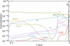 |
Fig. B.1 Results for noEX model in region A. Compare with Fig. 7 showing the standard case. |
| In the text | |
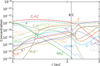 |
Fig. B.2 Results for noEX model in region B. Compare with Fig. 9 showing the standard case. |
| In the text | |
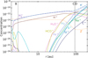 |
Fig. B.3 Results for noEX model in region C. Compare with Fig. 9 showing the standard case. |
| In the text | |
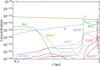 |
Fig. B.4 Results for EX model in region A. Compare with Fig. 7 showing the standard case. |
| In the text | |
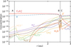 |
Fig. B.5 Results for EX model in region B. Compare with Fig. 9 showing the standard case. |
| In the text | |
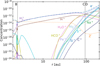 |
Fig. B.6 Results for EX model in region C. Compare with Fig. 11 showing the standard case. |
| In the text | |
Current usage metrics show cumulative count of Article Views (full-text article views including HTML views, PDF and ePub downloads, according to the available data) and Abstracts Views on Vision4Press platform.
Data correspond to usage on the plateform after 2015. The current usage metrics is available 48-96 hours after online publication and is updated daily on week days.
Initial download of the metrics may take a while.