| Issue |
A&A
Volume 666, October 2022
|
|
|---|---|---|
| Article Number | A37 | |
| Number of page(s) | 10 | |
| Section | Numerical methods and codes | |
| DOI | https://doi.org/10.1051/0004-6361/202244136 | |
| Published online | 03 October 2022 | |
Fluid simulation of dust-acoustic solitary waves in the presence of suprathermal particles: Application to the magnetosphere of Saturn★
1
Department of Mathematics, Khalifa University of Science & Technology,
PO Box 127788,
Abu Dhabi, UAE
e-mail: This email address is being protected from spambots. You need JavaScript enabled to view it.
This email address is being protected from spambots. You need JavaScript enabled to view it.
2
Indian Institute of Geomagnetism,
New Panvel,
Navi Mumbai
410-218, India
3
Space and Planetary Science Center, Khalifa University of Science & Technology,
PO Box 127788,
Abu Dhabi, UAE
Received:
28
May
2022
Accepted:
29
July
2022
Abstract
The observation of dust in the rings of Saturn by instruments on board the Voyager 1, Voyager 2, and Cassini missions triggered our interest in exploring the evolution of electrostatic dust acoustic waves (DAWs) in the Saturnian magnetospheric dusty plasma. The salient features of dust-acoustic electrostatic solitary waves have been examined by means of numerical simulations that adopted a fluid algorithm. We considered highly energetic non-Maxwellian ion and electron populations, in combination with inertial dust. The ions and electrons were modeled by kappa distributions to account for the long-tailed particle distribution featuring a strong suprathermal component. At equilibrium, the initial density perturbation in the dust density was used to trigger the evolution of DASWs propagating in non-Maxwellian dusty plasma. Our main focus is to determine the comprehensive role of the dust concentration and the suprathermal index (kappa) of the ion and electron populations in the generation and evolution of DASWs. These simulation results are thought to be relevant for (and applicable in) existing experimental data in space, especially in the magnetosphere of Saturn, but also in other planetary plasma environments that are presumably characterized by the presence of charged dust.
Key words: plasmas / waves
The data underlying this article will be shared on reasonable request to the corresponding author.
© K. Singh et al. 2022
 Open Access article, published by EDP Sciences, under the terms of the Creative Commons Attribution License (https://creativecommons.org/licenses/by/4.0), which permits unrestricted use, distribution, and reproduction in any medium, provided the original work is properly cited.
This article is published in open access under the Subscribe-to-Open model. This email address is being protected from spambots. You need JavaScript enabled to view it. to support open access publication.
1 Introduction
Dust is an inevitable component in space and astrophysical environments. The past few decades have seen a growing interest in the physics of dusty plasma and focused on the investigation of associated (e.g., electrostatic) modes and instabilities because their role in space and astrophysical plasmas is important (e.g., in planetary rings and comet tails; Goertz 1989; Horanyi & Mendis 1986a,b; Verheest 1996) and in laboratory plasmas (e.g., plasma devices, fusion devices, solar cells, and semiconductor chips; Samarian et al. 2001, 2005; Adhikary et al. 2007). A dusty plasma is essentially a traditionally considered (electron-ion) plasma enriched by massive charged-dust particles. The charge of the dust grains may be either positive or negative, and their size may vary from tens of nanometers (nm) to hundreds of microns (µm). The dynamics of these massive charged particles occurs on considerably slower timescales than for ordinary plasma because of their significant mass (which may exceed the ion mass a billion times, or even more). The existence of dust grains mainly gives rise to two novel low-frequency modes: the dust acoustic mode (Rao et al. 1990), and the dust-ion-acoustic mode (Shukla & Silin 1992). Dust-acoustic waves are low-frequency waves in which the restoring force arises from the pressure of the electrons and ions, while the inertia to support wave propagation stems from the dust mass. These waves can be visualized in the laboratory (Barkan et al. 1995). Numerous investigations to explore the characteristics of nonlinear dust acoustic waves in various plasma environments have been reported to date (Rao et al. 1990; El-Taibany & Kourakis 2006; Saini & Kourakis 2008; Ghosh et al. 2012; Singh et al. 2018; Singh & Saini 2020).
Various spacecraft missions and satellite observations have corroborated the extensive presence of energetic particle populations in various space environments, resulting in measured distributions deviating from the thermal (Maxwell-Boltzmann) distribution and in fact resulting in a long tailed (non-Maxwellian) distribution with strong relative weight in its suprathermal component (Liu & Du 2009). Suprathermal particles have been observed in the Earth magnetosphere (Feldman et al. 1975), in the solar wind, in the auroral zone (Lazar et al. 2008; Mendis & Rosenberg 1994), and also in the magnetosheath (Masood et al. 2006). Vasyliunas was the first to adopt a kappa velocity distribution as an empirical formula to fit data from the OGO 1 and OGO 3 spacecraft in the terrestrial magnetosphere (Vasyliunas 1968), thus successfully modeling the long-tailed behavior in the suprathermal component of the observed distribution. Since then, it has been employed to fit particle distributions observed in Saturn, in the solar wind (Armstrong et al. 1983), and in the magnetospheres of Earth and Jupiter (Leubner 1982). The magnetosphere of Saturn is typically characterized by a kappa distribution with low values of the kappa index (κ ~ 2–6, usually; Schippers et al. 2008). For a very high spectral index (i.e., κ → ∞), the non-Maxwellian kappa distribution approaches the standard expression for the Maxwell-Boltzmann distribution. Data from the Voyager 1 and 2 spacecraft in the magnetosphere of Saturn established that ions follow a power law at high energies. Krimigis et al. (1983) adopted the suprathermal distribution to fit ion data in the magnetosphere of Saturn, with spectral index values ranging from 6 to 8. The Cassini team collected data from Saturn that covered distances ranging from 5.4 to 18 Rs, where Rs is the Saturn radius (Rs ≈ 60 268 km). These observations established that the observed electron data from the magnetosphere of Saturn can be well fitted by a kappa distribution (Schippers et al. 2008).
The Radio and Plasma Wave Science (RPWS) instrument on board Cassini has contributed a strong affirmation that charged dust particulates in the E-ring prominently interact with the Saturnian magnetospheric plasma (Wahlund et al. 2009). On the basis of data from grain sizes of 41 mm, it has been extrapolated that the sixth-largest moon of Saturn, Enceladus, emits a dust toroid that spreads to create most of the E-ring. The density of these large dust grains is about 10−7 cm−3, which is lower than the surrounding plasma disk. Moreover, the dust population obeys a  power law (with m ~ 4–5; Kempf et al. 2005), where rd is the radius of dust grains; the dust density therefore escalates more sharply for smaller dust particles, hence the E-ring is much influenced by submillimeter-sized grains. The charge of the dust in the E-ring was measured by the dust Cosmic Dust Analyzer (CDA) instrument on board Cassini to be a few volts negative inside 7 Rs (Kempf et al. 2006). Electrostatic coupling of micron-sized dust has also been conjectured in the inner rings of the Saturn spokes (Wahlund et al. 2009). Cassini Radio and Plasma Wave Science Wideband Receiver (WBR) data clearly detected a high percentage of bipolar-type electrostatic solitary waves (ESWs) up to 10 Rs in 2004–2008. This location is compatible with the high-density part of the Saturn E ring and orbit regions of Enceladus (Pickett et al. 2015).
Over the past few decades, various investigations have focused on the characteristics of ultra-low frequency dust-acoustic (DA) ESWs in non-Maxwellian multicomponent plasma composed of electrons and ions (Rao et al. 1990; Saini & Kourakis 2008; Ghosh et al. 2012; Singh et al. 2018; Singh & Saini 2020), relying on either perturbative or nonperturbative techniques with different assumptions in order to obtain analytical solutions representing DA ESWs. These techniques have been valuable in providing static prediction of waveforms, but they inherently fail to address the generation mechanism or the propagation dynamics of nonlinear solitary waves. Computer simulation as the most efficient tool are therefore employed to understand the dynamical evolution of nonlinear solitary waves, in fact based on theoretical predictions from deterministic (analytical) models as inspiration for initial conditions or to predict the qualitative form (the shape) of the solitary excitations.
In a series of recent studies, Kakad et al. (2013, 2014, 2016) employed fluid simulations to describe the dynamics of ion-acoustic solitary waves (IASWs) in a classical (nonrelativistic) electron-ion fluid plasma. Based on a Gaussian initial density perturbation profile in the short- and (independently) long-wavelength regimes, their simulations have successfully validated the widely used Sagdeev pseudopotential nonlinear analyis technique, based on plasma fluid theory. Later, Lotekar et al. (2019) developed an efficient Poisson solver by adopting the successive over relaxation method in a numerical simulation of a plasma comprising kappa-distributed electrons (Lotekar et al. 2016, 2017). More recently, Singh et al. (2020, Singh et al. 2021) explored the evolution of IASWs interacting with the pulsar wind by employing fluid simulations. In the study at hand, we have used a similar technique to develop a first fluid code, customized to modeling dust acoustic solitary waves in the dusty plasma environment of Saturn. Our results can be compared against experimental data in space plasmas, especially in the magnetosphere of Saturn and in cometary tails (Goertz 1989).
The objective of this study is to examine the nonlinear evolution of dust-acoustic solitary waves (DASWs) in Saturnian magnetospheric dusty plasma. We have undertaken a series of computer simulations in order to explore how the dust density and the electron suprathermality (deviation from the Maxwellian equilibrium) affect the propagation characteristics of DASWs. This paper is organized as follows. The fluid model and numerical schemed adopted in the simulation algorithm are given in Sect. 2. The simulation results are discussed in Sect. 3. The salient features of DASWs are given in Sect. 4. The plasma conditions and validation of observations of ESWs in magnetosphere of Saturn are given in Sect. 5. Finally, we summarize our results and conclude this study in Sect. 6.
2 Plasma model
We considered a plasma comprised of electrons and ions, both considered to be in a non-Maxwellian state, in addition to negatively charged inertial dust particles (with charge −Zde) to examine the evolution of DA solitary waves (SWs) in the magnetosphere of Saturn. In the standard way, Zd is the dust grain charge state, while e denotes the elementary (electron absolute) charge. Neutrality at equilibrium was assumed, so that ni0 = Zdnd0 + ne0, where ns0 for (s = e, i, d) denotes the unperturbed number density of the respective plasma species. The ambient magnetic field was neglected for simplicity. Physically speaking, this is tantamount to considering wave propagation along a uniform magnetic field (B) (because the Larmor force v × B possesses no component along B).
The model was governed by the following fluid (continuity, momentum) equations for the inertial dust fluid:
 (1)
(1)
 (2)
(2)
in addition to Poisson’s equation,
 (3)
(3)
where nd and ud denote the dust fluid density and velocity, respectively, ϕ is the electrostatic potential, and md is the dust mass. The thermal pressure gradient force in the momentum Eq. (2) was neglected because we assumed cold dust for simplicity. The ion and electron components both follow non-Maxwellian (kappa-type) distributions, hence their densities are given by
 (4)
(4)
and
 (5)
(5)
respectively. In the latter relations, Ti and Te denote the ion and electron temperature, respectively, while qi = e is the ion charge, and qe = −e is the electron charge. In this fluid simulation, we considered a discrete system to evaluate the numerical solution of Eqs. (1)–(3).
We comment on the numerical algorithm we adopted. The spatial derivatives in the fluid Eqs. (1)–(2) were numerically estimated by using the fourth-order finite difference formula (Kakad et al. 2014, 2016; 2016, 2017, 2019)
 (6)
(6)
where Θℓ denotes any of the plasma state variables at the ℓth grid point. The accuracy of this formula is ~∆x4. The leap-frog method with an accuracy of ∆t2 was adopted for the time integration of Eqs. (1)–(2). To minimize the numerical error, we employed the fourth-order compensated filter (Kakad et al. 2014, 2016; 2016, 2017, 2019; Singh et al. 2020, 2021), which was used in earlier studies, given by equation
 (7)
(7)
where  denotes the filtered quantity at the ℓthth grid point. We adopted periodic boundary conditions in our fluid simulation. The values of ∆x and ∆t were determined in such a way that the Courant-Friedrichs-Lewy (CFL) condition (i.e.,
  ) was always fulfilled for a stable computation. In each simulation run, ud = 0 at t = 0 and ϕ = 0. Suitable values of the background dust and electron and ion densities (at equilibrium) were chosen, so that Zdnd0 + ne0 = ni0. To excite electrostatic (dust-acoustic) waves, we used an initial density perturbation (IDP) δnd with a standard Gaussian form (Kakad et al. 2014; Lotekar et al. 2016), that is, nd = nd0 + δnd. The dust equilibrium density is expressed as
![Mathematical equation: $ {n_{\rm{d}}} = {n_{{\rm{d0}}}} + {\rm{\Delta }}n\,\,\exp \left[ { - {{\left( {{{x - {x_c}} \over {{l_0}}}} \right)}^2}} \right], $](/articles/aa/full_html/2022/10/aa44136-22/aa44136-22-eq11.png) (8)
(8)
where ∆n and l0 are the amplitude and width of the perturbation, nd0 is the dust (equilibrium) density and xc is the center of the simulation box. The suprathermal ions and electrons densities given in Eqs. (4)–(5) are functions of ϕ, as well as of the κe and κi parameters. It may be noted that there are no ion and electron continuity equations to update their values at the next time step. To compute the electron and ion densities at time step t + ∆t, we need information of ϕ. Conversely, to compute ϕ, we need information on the densities. Therefore, we employed an iterative approach by using the successive-over-relaxation (SOR) method (Lotekar et al. 2019; Singh et al. 2020, 2021) to solve the Poisson equation. The initial value of the electrostatic potential at the previous time step is an estimate (a guess), which is substituted in Eq. (3), and then solved for the electrostatic potential. After every iteration, the new value of φ is considered as a new guess, and the procedure is repeated until it satisfies the termination criteria.
We executed the SOR method in Poisson’s equation as follows:
![Mathematical equation: $ \matrix{ {\bar \phi _j^{r + 1}} \hfill & = \hfill & {\left( {1 - \zeta } \right)\phi _j^r + {\zeta \over 2}\left[ {{\rm{\Delta }}{x^2}} \right.\left\{ {{n_{{\rm{i0}}}}} \right.{{\left( {1 + {{{q_{\rm{i}}}{\phi ^r}} \over {\left( {{\kappa _{\rm{i}}} - {3 \over 2}} \right){k_{\rm{B}}}{T_{\rm{i}}}}}} \right)}^{ - {\kappa _{\rm{i}}} + {1 \over 2}}} + \phi _{j + 1}^r} \hfill \cr {} \hfill & {} \hfill & {\left. {{{\left. { + \phi _{j - 1}^{r + 1} - {n_{{\rm{e}}0}}{{\left( {1 + {{{q_{\rm{e}}}{\phi ^r}} \over {\left( {{\kappa _{\rm{e}}} - {3 \over 2}} \right){k_{\rm{B}}}{T_{\rm{e}}}}}} \right)}^{ - {\kappa _{\rm{e}}} + {1 \over 2}}} - {Z_{\rm{d}}}{n_{\rm{d}}}} \right\}}_j}} \right],} \hfill \cr } $](/articles/aa/full_html/2022/10/aa44136-22/aa44136-22-eq12.png) (9)
(9)
Here, j and r represent the grid point and the iteration number, respectively, and ζ is a relaxation parameter in the SOR method. The iteration process in the simulation terminated when |ϕr − ϕr+1| <τ.
We selected τ = 10−5 and ζ = 0.7 for all runs. This tolerance level has been found to allow stable numerical computation in the Poisson solver by reducing the numerical error. In the next section, we present the results obtained from the simulations.
3 Simulation results
Adopting values from Yaroshenko et al. (2007), the magnetosphere of Saturn is characterized by the following typical values: the electron density is approximately ne ≃ 2–45cm−3; ion density ni ≃ 1–20 cm−3; dust density nd ≃ 10−3–10−1 cm−3; dust charge Zd ≃ 1–100; electron temperature Te ~ 1–10 eV; dust temperature Td ≃ 0.01 eV, and kappa indices κi,e ≃ 2–6 (Schippers et al. 2008; Krimigis et al. 1983). Based on these parameters, we have chosen the plasma parameters for our simulation as ne = ni ≃ 20 cm−3, nd ≃ 0.08–0.18 cm−3, Zd ≃ 100, Te ~ 10 eV, Td ≃ 0.01 eV, Ti = 1 eV, Ki,e ≈ 2–6 for suprathermal and κi,e = 20 (quasi-Maxwellian). These values are normalized and then provided as input to the simulations for the computational convenience. The velocity, density, space and time variables are respectively normalized with the ion thermal velocity, Vthi = (kBTi/mi)1/2 = 9.8 km s−1, the ambient plasma density n0 = 20 cm−3, the characteristic length λD = (ϵ0kBTi/n0e2)1/2 = 1.66 m, and the inverse of the ion plasma frequency (the plasma period)  . Furthermore, the electrostatic potential is normalized by (
 ) in Volt units. Therefore, in all figures in this paper, the dust density is scaled by n0, time is scaled by the ion plasma period
  , velocity is in units of
  , and space is in units of λD.
In all simulation runs, the normalized parameters are considered as follows; grid spacing ∆x = 0.05, the time interval is ∆t = 0.0008; IDP amplitude ∆n = 0.05, IDP width l0 = 1, Zd = 100, md = 1000mi,  , Td = 0.1Ti and Te = 10 Ti have been chosen. Particularly for nd = 0.005 and ne = 0.5. Here, Zdnd0 + ne0 = ni0 = n0 = 1. The plasma frequencies for the components of relevance to our study are ωpd = 0.2236 ωpi and ωpe = 30.299 ωpi, and the corresponding Debye lengths are λDd = 0.0447 λD and λDe = 4.472 λD, respectively. Various input parameters considered for different simulation runs are summarized in Table 1 in normalized units. We have examined the effect of the kappa index (value) for both electrons and ions, as well as of the dust density, on the evolution of dust-acoustic solitary waves.
As a representative example, we shall discuss in the following the propagation of DASWs with data from simulation run 1(ii).
3.1 Generation and evolution of stable DASW pulses
Figure 1 shows a series of snapshots of the course of the DASW evolution, when the background density of inertial dust was perturbed by superimposing an IDP. At the initial time step (i.e., t = 0), quasi-neutrality at equilibrium causes the electrostatic potential in the system to be zero (see Fig. 1a). When an IDP (perturbation) is introduced in the system, a finite potential (of negative polarity, due to the negatively charged dust) is formed at the first time step through charge separation, as shown in Fig. 1b. The finite potential (perturbation) alters the ion and electron densities. This initial potential structure is unstable and evolves with time. In this simulation, the thermal velocities of ions and electrons exceed the thermal velocity of dust (Vthd ≪ Vthi ≪ Vthe). In this plasma, the electrons and ions provide the restoring force through their higher thermal velocity, whereas the dust provides the inertia needed to sustain low-hrequency electrostatic (dust-acouttic) oscillations in plasma. During the inisial time steps, trie potential amplitude slowly decreases with time. Aftes dropping to a specific amplitude (value), ttte peak; erf trie potential pulse bifurcates and the pulse splits, as shown in Figs. 1c and d. Two identical DASW pulses are thut formgd in tinte, as shown in Fig. 1e. hhete DASWs (pulses) propagate at the phase speed Vp in opposite directions, as shown in Fig. 1f, fotlowed by smaller amplitude dust acoustic (DA) oscillations; see Fig; 1f. These stable pultes are clearly visible in Fiat 1f. They are DA solitonr propagating at constant speed and sustaining a constant amplitude immediately aftet their formation at ωpit = 640. In an analogous series of diagrams, the corresponding bipolar electric field pulses are illuitrated in Fig. 2 at the same time steps.
Input parameters used in all (19) simulation runs for different combinations of nd, κi, and κe.
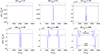 |
Fig. 1 Series of snapshots from trie simulation, with data from run 1 (ii), depict the evolution of dust acoustic solitary waves in non-Maxwellian dusty plaama. (a) At equilibrium for t = 0, quasi-neutrality is aatisfied. (b) Formation of an electrostatic potential pulse at the first Sime step. (c and d) Splitting; of the electrostatic potential pulse into two DASW puises. (e) Formation of two indistinguishable DASW pulses. (f) The two stable DASW pulses propagate in opposiie duections with the same speed Vp. The parameters used in this run are given in Table 1. |
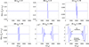 |
Fig. 2 Series of snapshots from the simulation (same data from run as in Fig. 1) depict the evolutionof the corresponding bipolar electric field waveform. Different panels show the formation of bipolor electric field profilet corresponding to Fig. 1. |
3.2 Spatio-temporal variation of DASW pulse s
We have examined the influence of the dust concentration and of the electron and ion superthermality (deviation from thermal equilibrium), reflected in the (respective vatue of the) spectral index k, on the formotion of DASWs (electrostatic pulses) through the spatio-temporal variation of the electrostatic potential. This is illustrated in Figs. 3 and 4. The initially formed DA pulse is clearly seen to split into two identical DA solitary waves (SWt). In each simulation run, the two identical DASW pulses propagate in opposite directions. The propagation spe-d and the maximum amplitudet of the DASW (pulse) pairs thus created diffet between successivf runs, depending on the chosen plasma parameter sets (values). The role of these alasma parameters in the evolutionary characteristics of the DASWs is discutsed below.
The generation andpropagafion oi DASW pulses is depicted in Figs. 3a-d for different value of the dust density (nd). An increase in the dust concentration clearly leads to an decrease in the amplitude ot DASW pulses. DASW pulses generated in plasma with a higher dust concentration are visibly fastes fhat is, the phase speed is an tncreasing function of the dust density, as predicted in theory (we recall that nonlinear solitary waves are superaraoutic, i.e., they propagate above the sound, here, the dust-acoustic, speed).
In order to investigate the impact of suprathermal particles on (he background, mantfested via non-Maxwellian particle distribution, we observed the dynamical characteristics of the generated negative-polarity DASW pulses upon choosing dtfter-en- values of the spectral indices κi and κe, forthe ions and the electrons, respectively. The evolution of the electrostatic potential is shown in Fits. 4a–d tor different values of κe or/and κj. The phase speed and the maximum amptitude of DA SW (putses) decrease to lower values tor lower values ot k (i.e., with a htgher concentration of suprathermal particles) Uhan in the runs with higher values of κ (see Figs. 4a-d). This is because a stronger suprathemial electron or/and ion component modifies -he most probable thermal speed (Hellberg et al. 2009) for the respective species (contributing to a notification rathe electrostatic charge distribution in the background), which in turn affects the speed and tho amplitude of DASW pulses; the observed change agrees with the theory (Saini & Kourakis 2008)). Hence, for thf suprathermal electrons/ions (i.e., for lower κe and κi), the phase speed of DASW pulseo is lowes than in tho thermal (Maxweilian) plasma case (i.e., for higher κe and κj). Furthermore, a comparison among the various subpanels in Fig. 4 implies that tte tnfluence ot suprathermal ions on the characteristics of DASW pulses is stronger than that of the suprathermal electrone Energetic ions appear to accelerate the DA mode more efficiently Finally, comparing either of Figs. 4b and c with Fig. 4d, bottom right, as reference (as the quasi-Maxwellian plasma state, say), we see that the wave properties aro affected when the ton spectral index κj is changed, rather than its eleetron counterpcrt (κe). The reason may be that lighter electrons are ettier to tíiermalize, while ions (ot opposite chargo to the dust) seem to affect the eleetrostatic background (and the Debye cloud surrounding the negative dust grains) in a stronger manner.
3.3 Dispersion characteristics of DASW pulses
We have computed the pmrer spætrum over space and time by using the fast Fourier tran-formation (FFT) of the electrostatic potential to recognise the variom wave modes that hrave been excited and evolve in the given plasmra (numerical experiment). From Eqs. (1)–(5), the linear dispersion retation of DAWs in suprathermal dusty ptasma can be written as
![Mathematical equation: $ {\omega ^2} = {{{k^2}} \over {{m_{\rm{d}}}}}\left[ {{{Z_{\rm{d}}^2{n_{{\rm{d0}}}}{T_{\rm{i}}}{T_{\rm{e}}}} \over {{n_{{\rm{i0}}}}{T_{\rm{e}}}\left( {{{{\kappa _{\rm{i}}} - 1/2} \over {{\kappa _{\rm{i}}} - 3/2}}} \right) + {n_{{\rm{e0}}}}{T_{\rm{i}}}\left( {{{{\kappa _{\rm{e}}} - 1/2} \over {{\kappa _{\rm{e}}} - 3/2}}} \right)}}} \right]. $](/articles/aa/full_html/2022/10/aa44136-22/aa44136-22-eq19.png) (10)
(10)
Figures 5a-d depicts the dispersion characteristics of DASWs obtained from different simulation run- for different valuras of the dust density. A higher dust density leads to faster pukes: the depicted pulse move with phase speed equal to 0.13, 0.14, 0.15, and 0.16 [Vthj] when nd is 0.005, 0.006, 0.007, and 0.008, respectively. The dispersion relation obtained from the simulation agrees well with the dispersion relation estimated from linear theory (i.e., Eq. (10)), which is plotted as dashed black curves in Figs. 5 and 6.
Figures 6a-d shows the dispersion plot of DASW excitations for different levels of superthermality of electrons and ions. The increase in the kappa indices results in a higher phase speed. We also emphasize that the power distributed among the fe-range of values is higher for the Maxwellian case than for the suprathermal case. The dispersion relation obtained from the simulation is well fitted by the linear dispersion (Eq. (10)), shown as the dashed curve. Concluding this section, we have shown that the frequency spectrum and the wave propagation characteristics obtained from the simulations agree very well with the theory.
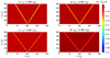 |
Fig. 3 Spatio-temporal evolution of the electrostatic potential for different values of the dust density (nd), based on data from run 1 (ii–v). The two slanted yellow color bands in each panel correspond to the DASW pulses. The darker (and slower) regions following them are linear electrostatic oscillations. |
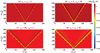 |
Fig. 4 Spatio-temporal evolution of the electrostatic potential for different values of the spectral index of electrons and ions, i.e., κe and κi respectively. Panel a was plotted from run 2(i), panel b from run 3(vi), panel c from run 2(vi), and finally, panel d was plotted from run 4. The plasma parameters of these runs are given in Table 1. A comparison of panels a and d suggests that highly suprathermal electrons and/or ions (i.e., for lower values of κ) correspond to smaller amplitude DASW pulses, in comparison with weakly suprathermal (e.g., quasi-Maxwellian) electrons and/or ions. |
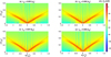 |
Fig. 5 Frequency-wavenumber (ω–k) diagram for different values of the dust density (nd) based on data from runs 1(ii–v). The dashed black lines are plotted from the linear dispersion of DA waves in each case, based on Eq. (10). The depicted ω–k plots were generated by using data in the time interval ωpit = 0–640. The phase speeds of DASWs obtained as 0.13, 0.14, 0.15 and 0.16 [Vthi] when nd is 0.005, 0.006, 0.007, and 0.008, respectively. |
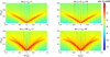 |
Fig. 6 Frequency–wavenumber (ω–k), based on the simulation runs for different values of the suprathermal indices of electrons and ions (κe and κi). The dashedblack lines are plotted from the linear dispersion relation of DA waves from Eq. (10) in each case. Panel a was plotted based on data from run 2(i), panel b from run 3(vi), panel c Srom run 2(vi), and panel d from run 4. The estimated phase speeds of DASW pulses are 0.13, 0.14, 0.20, and 0.21 [Vthi] in panels a, b, c, and d, respectively. The plasmaparameters of these runs are given in Table 1. The above ω–k plots are generated using data from the time interval ωpit = 0–640. |
4 Characteristics of DASWs: Theory versus simulation
In this section, we summarize Sagdeev’s pseudopotential technique as adopted to our dusty plasma fluid model. Anticipating stationary profile solutions, we may transform Eqs. (1)–(5) into a stationary frame, that is, η = x − Mt, moving at the phase speed Vp, here to be denoted by M. Although as a matter of common practice, the symbol M (standing for the Mach number in acoustics) is adopted, the solitary wave speed here denoted by M is not the true Mach number because the characteristic speed scale by which it has been normalized is not the true sound speed in the given plasma configuration. (The true sound speed is given by Eq. (13); as expected, the solitary waves in fact propagate at a slightly higher speed.) Solving Eqs. (1) and (2) for the perturbed dust density as a function of the electrostatic potential ϕ, then substituting in Poisson’s equation and eventually integrating, by assuming appropriate boundary conditions for the localized disturbances (guaranteeing, i.e., that the plasma remains at equilibrium far from the solitary wave) along with the conditions that ϕ = 0 and dϕ/dη = 0 at η → ±∞, we obtain a pseudo-energy integral in the form
 (11)
(11)
In this expression, S (ϕ) is a (real) pseudopotential function given by
![Mathematical equation: $ \matrix{ {S\left( \phi \right)} \hfill & = \hfill & {{{{n_{{\rm{d0}}}}{m_{\rm{d}}}{M^2}} \over {{_0}}}\left[ {1 - {{\left( {1 + \left( {{{{Z_{\rm{d}}}{\rm{e}}} \over {{m_{\rm{d}}}}}} \right){{2\phi } \over {{M^2}}}} \right)}^{1/2}}} \right]} \hfill \cr {} \hfill & {} \hfill & { + {{{n_{{\rm{e0}}}}{k_{\rm{B}}}{T_{\rm{e}}}} \over {{_0}}}\left[ {1 - {{\left( {1 - {{e\phi } \over {\left( {{\kappa _{\rm{e}}} - 3/2} \right){k_{\rm{B}}}{T_{\rm{e}}}}}} \right)}^{ - {\kappa _{\rm{e}}} + 3/2}}} \right]} \hfill \cr {} \hfill & {} \hfill & { + {{{n_{{\rm{i0}}}}{k_{\rm{B}}}{T_{\rm{i}}}} \over {{_0}}}\left[ {1 - {{\left( {1 + {{e\phi } \over {\left( {{\kappa _{\rm{i}}} - 3/2} \right){k_{\rm{B}}}{T_{\rm{i}}}}}} \right)}^{ - {\kappa _{\rm{i}}} + 3/2}}} \right].} \hfill \cr } $](/articles/aa/full_html/2022/10/aa44136-22/aa44136-22-eq21.png) (12)
(12)
The nonlinear analysis predicts a lower bound for M, say Mmin, below which solitary wave solutions cannot be formed; this limit, given as
![Mathematical equation: $ {M_{\min }} = \sqrt {{{Z_{\rm{d}}^2{n_{{\rm{d0}}}}} \over {{m_{\rm{d}}}\left[ {{{{n_{{\rm{e0}}}}\left( {{\kappa _{\rm{e}}} - 1/2} \right)} \over {{k_{\rm{B}}}{T_{\rm{e}}}\left( {{\kappa _{\rm{e}}} - 3/2} \right)}} + {{{n_{{\rm{i0}}}}\left( {{\kappa _{\rm{i}}} - 1/2} \right)} \over {{k_{\rm{B}}}{T_{\rm{i}}}\left( {{\kappa _{\rm{i}}} - 3/2} \right)}}} \right]}}} = {V_{\rm{p}}}, $](/articles/aa/full_html/2022/10/aa44136-22/aa44136-22-eq22.png) (13)
(13)
essentially coincides with the (dust-acoustic) sound speed, as obtained from linear theory. Solitary waves are indeed superacoustic (supersonic).
An upper bound Mmax also exists above which no solitary waves exist. This is obtained by solving the following equation numerically
![Mathematical equation: $ \matrix{ {{{{n_{{\rm{d0}}}}{m_{\rm{d}}}M_{\max }^2} \over {{_0}}}} \hfill & + \hfill & {{{{n_{{\rm{e0}}}}{k_{\rm{B}}}{T_{\rm{e}}}} \over {{_0}}}\left[ {1 - {{\left( {1 - {{{m_{\rm{d}}}M_{\max }^2} \over {{Z_{\rm{d}}}\left( {2{\kappa _{\rm{e}}} - 3} \right)}}} \right)}^{ - {\kappa _{\rm{e}}} + 3/2}}} \right]} \hfill \cr {} \hfill & + \hfill & {{{{n_{{\rm{i0}}}}{k_{\rm{B}}}{T_{\rm{i}}}} \over {{_0}}}\left[ {1 - {{\left( {1 + {{{m_{\rm{d}}}M_{\max }^2} \over {{Z_{\rm{d}}}\left( {{\kappa _{\rm{i}}} - 3/2} \right)}}} \right)}^{ - {\kappa _{\rm{i}}} + 3/2}}} \right] = 0,} \hfill \cr } $](/articles/aa/full_html/2022/10/aa44136-22/aa44136-22-eq23.png) (14)
(14)
thus guaranteeing the reality of all state variables in the dynamical problem.
By using relations (13) and (14), we have established the existence diagram of DA solitons by varying the dust density and the ion and electron superthermality indices; this region is shown, in the latter three cases, as the shaded region in Fig.7. We attempted to validate our fluid simulations by locating them as ‘points inside the existence regions obtained from nonlinear theory. Figure 7 shows the variation in solitary wave speed (M) with respect to the dust density (nd) and the superthermality indices (κi and κe). The green asterisks in this figure correspond to DA pulse speed values as obtained from the simulation. This (speed) was calculated in the region where these pulses are sufficiently stable, that is, when the solitary pulse width and amplitude were practically constant. Figure shows that the observed pulses were weakly superacoustic in that their speed was situated in the vicinity (above) the sound speed (i.e., the lower bound Mmin). The pulse speed is found to be an increasing function of the dust density and of the suprathermal indices (both).
We also measured the maximum amplitude of the solitary waves at their stable stage in all simulation runs. These amplitudes were compared to the amplitudes obtained from the theory. To do this, we took the speed of the pulse(s) obtained from the simulation as an input to solve Eq. (11) numerically. The numerical solution of this equation gives the spatial profile of ϕ, from which the corresponding amplitude and width of the DA soliton were calculated. Here, by width we mean the peak-to-peak spatial separation in the bipolar electric field pulse. Figure 8 illustrates the variation in absolute value of the peak amplitude 〈|ϕmax|〉 estimated from the theory and simulation with dust density and kappa indices. The amplitude is given by blue asterisks in this figure from the simulation data, while the circles depict the amplitudes obtained from the theory. The simulation results clearly agree very well with the predictions from nonlinear fluid theory. Finally, the peak amplitude of negative-polarity DASW pulses decreases with the dust density (i.e., more dust in the plasma results in a lower amplitude). The peak amplitude decreases with lower κi and κe, that is, it becomes weaker as the background particle density deviates from the Maxwellian.
Figure 9 illustrates the variation in pulse width (theory vs. simulation) with the dust density and with the kappa indices. The width represented by blue asterisks in this figure is from the simulation data, while the circles represent the amplitudes obtained from the theory. The simulation results clearly agree with the predictions of the nonlinear fluid theory. Qualitatively speaking, the pulse width increases with the dust density, while it decreases for smaller κi and κe: Pulses will therefore be wider for a stronger deviation of the suprathermal component from the Maxwellian picture, and they will also be wider when the plasma contains more dust.
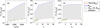 |
Fig. 7 Variation in average solitary wave phase speed 〈Vp〉 as measured numerically for different values of nd (panel a), κi (panel b), and κe (panel c). The remaining parameter values used in the simulation are given in Table 1. The panels are plotted from the datasets of simulation run 1(i–vi), run 2(i–vi), and run 3(i–vi). |
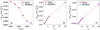 |
Fig. 8 Variation in average peak amplitude 〈|ϕmax|〉 of the solitary wave for different values of nd (panel a), κi (panel b), and κe (panel c). The remaining parameter values used in the simulation are listed in Table 1. These panels are plotted from the simulation datasets of run 1(i–vi), run 2(i–vi), and run 3(i–vi). |
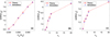 |
Fig. 9 Measured peak-to-peak spatial separation of the bipolar electric field pulse width versus nd (panel a), κi (panel b), and κe (panel c). The remaining parameter values used in the simulation are listed in Table 1. These panels are plotted from the simulation datasets of run 1(i–vi), run 2(iûvi), and run 3(i–vi). |
5 Plasma conditions and validation in Saturn’s magnetosphere
In their 3D simulations, Mitchell et al. (2005) distinguished a wide ring of dust cloud recorded into retrograde orbits extending upto 9RS with a thickness of 3RS. They confirmed the existence of 0.1 µm sized dust particles with peak density 3 × 10⁻¹⁵ cm−3, as observed by the Cassini spacecraft. The Cassini mission has provided a large number of in situ observations that have been adopted in many dusty plasma models. The powerful combination of 12 on board instruments has provided unprecedented data on the rings and the dynamical processes, composition, density, and size distribution. Furthermore, the E-ring in magnetosphere of Saturn is an ideal laboratory for studying the charging processes of dust particles and spacecraft. Fed by ice particles from the volcanically active moon Enceladus, the E ring spans from about 3Rs to orbit of Titan at 20 Rs in magnetosphere of Saturn (Hsu et al. 2013). In Maxwellian plasma where photoemission is usually ignored, an object easily gets negatively charged due to the dominant electron current. Taking account the dust electrostatic charge measurements performed by the Cassini Cosmic Dust Analyser in the E ring, Kempf et al. (2006) showed that the dust potential is about −2 V near Enceladus (4 Rs) and becomes positive outside the orbit of the moon Rhea (8.7Rs). These grain charge measurements are in good agreement with the charging calculation based on Cassini measurements. This result describes that in the dense Enceladus torus the electron collection is dominant and results in negative dust potential. Moreover, the Cassini mission has provided data from Saturn covering distances ranging from 5.4–18 Rs, where Rs is the Saturn radius (Rs ≈ 60 268 km). Those observations established that electron/ion statistics from magnetosphere Saturn obey kappa distribution(s) with small values of the kappa index (κ ~ 2–6, usually; Schippers et al. 2008).
Pickett et al. (2015) analyzed the Cassini Radio and Plasma Wave Science Wideband Receiver (WBR) data explicitly for the existence of bipolar electrostatic solitary waves (ESWs) at 10 Rs and near Enceladus. They also provided the time series of the calibrated electric field data over 74 ms and 7 ms intervals from the Cassini RPWS WBR, 10 kHz and 80 kHz filter bandwidth, obtained on 16 January 2005 and on 9 October 2008, respectively. They observed several ESWs with amplitudes of about 100 µV m−1 up to about 140m Vm−1, and time durations of several tens of microseconds up to 250 µs. We have focused on a particular event (E5) observed by Cassini on 9 October 2008 over a 35 min period during an Enceladus encounter. In that event, the ESWs with peak-to-peak electric field amplitude was around 0.1–1.0 mV m−1 and the time duration was a few tenths of milliseconds are also observed. This was the first extended investigation of ESWs near Saturn from first principles, to our knowledge, in connection with Enceladus.
Our numerical simulation has provided the conditions for the spontaneous excitation of solitary waves in the form of bipolar electric field waveforms associated with negative polarity potential pulses, with maximum potential ϕmax ≈ 9–21 mV, maximum amplitude of the E-field bipolar waveform Emax ≈ 0.7–1.3 mV m−1, speed ≈ 1.2–2.1 km s−1, peak-to-peak electric field amplitude i.e., Epp = 2|Emax| = 1.4–2.6 mVm−1, peak-to-peak spatial separation of the bipolar electric field width ≈ 11–16 m and duration (=width/speed) ~7–9 ms. Basically, the pulse characteristics in the simulation depend on both initial density perturbation (IDP) and plasma parameters. Adopting a IDP with larger amplitude might have led to a reduced time duration of the pulse (Lotekar et al. 2016). The simulation run 1(vi) has provided good agreement with observations, in that the peak-to-peak electric amplitude ≈ 1.4 is more close to the observed profile i.e., around 1.0mV m−1 with smaller time duration in millisecond range. In nutshell, we can say that for higher dust density and highly suprathermal plasma the simulation results are closely agreed with space observations whereas for Maxwellian case(s) may differ which confirmed the presence of suprathermal charged particles in Saturn environments (Krimigis et al. 1983; Schippers et al. 2008). However, the characteristics of the localized waveforms obtained from our simulations are more or less - in order of magnitude – in good agreement with the recorded features of bipolar pulses observed by the Cassini mission near Saturn’s moon Enceladus (Pickett et al. 2015).
6 Conclusions
We have adopted advanced computer simulation techniques for the first time to investigate the dynamical evolution of dust-acoustic solitary waves in a plasma whose composition replicates the magnetosphere of Saturn based on observations. To do this, we relied on a fluid plasma model incorporating an inertial dust fluid, in addition to suprathermal (non-Maxwellian) electrons and ions. To the best of our knowledge, this is the first fluid simulation of electrostatic solitary waves (pulses) of the dust-acoustic type in non-Maxwellian dusty plasma, taking into account the role of the dust density as well as the particular aspects of the nonthermal electron and ion population(s).
The time required for the generation of stable DASW pulses is shorter the higher the value of (either of the) κ indices or/and the dust density. This fact suggests that DA solitary waves are generated much faster and are stabilized sooner (reaching a state of stationary profile) in thermal plasma than in suprathermal plasma. The characteristics of DASW pulses obtained from the fluid theory and simulations agree well. As the theory predicts, the peak amplitude increases with κe and κi and it decreases with nd. For higher dust density and highly suprathermal population, the simulation results are in close agreement with space observations by Cassini whereas for Maxwellian case it may differ which further confirmed the presence of suprathermal charged particles in Saturn environments.
We wished to shed some light on the dynamical evolution of low-frequency dust-related (dust acoustic) electrostatic solitary waves in the Saturnian environment, and in particular, to trace the dependence of their dynamics on the relevant plasma parameters (nonthermal electron and ion distribution, via κe and κi, and also on the dust concentration nd), elucidating the role of the latter on the conditions for existence of such structures. Our results are relevant for (and applicable in) existing experimental data in space, especially in the magnetosphere of Saturn, but also in other planetary plasma environments that are presumably characterized by the presence of charged dust.
Acknowledgements
K.S., A.K. and I.K. gratefully acknowledge financial support from Khalifa University of Science and Technology, Abu Dhabi UAE via the (internally funded) project FSU-2021-012/8474000352. Funding from the Abu Dhabi Department of Education and Knowledge (ADEK), currently ASPIRE UAE, via the AARE-2018 research grant ADEK/HE/157/18 is gratefully acknowledged. I.K. also acknowledges financial support from Khalifa University’s Space and Planetary Science Center under grant no. KU-SPSC-8474000336. This work was carried out during a visit by one of us (A.K.) to Khalifa University; the hospitality offered by the host is greatly acknowledged. The authors wish to acknowledge the contribution of Khalifa University’s high-performance computing (HPC) and research computing facilities to the results of this research.
References
- Adhikary, N. C., Bailung, H., Pal, A. R., Chutia, J., & Nakamura, Y. 2007, Phys. Plasmas, 14, 103705 [NASA ADS] [CrossRef] [Google Scholar]
- Armstrong, T.P., Paonessa, M. T., Bell, E. V., & Krimigis, S. M. 1983, J. Geophys. Res., 88, 8893 [NASA ADS] [CrossRef] [Google Scholar]
- Baluku, T. K., & Hellberg, M. A. 2008, Phys. Plasmas, 15, 123705 [NASA ADS] [CrossRef] [Google Scholar]
- Barkan, A., Merlino, R. L., & D’Angelo, N. 1995, Phys. Plasmas, 2, 3563 [NASA ADS] [CrossRef] [Google Scholar]
- El-Taibany, W. F., & Kourakis, I. 2006, Phys. Plasmas, 13, 062302 [NASA ADS] [CrossRef] [Google Scholar]
- Feldman, W. C., Asbridge, J. R., Bame, S. J., Montgomery, M. D., & Gary, S. P. 1975, J. Geophys. Res., 80, 4181 [Google Scholar]
- Ghosh, U. N., Chatterjee, P., & Roychoudhury, R. 2012, Phys. Plasmas, 19, 012113 [NASA ADS] [CrossRef] [Google Scholar]
- Goertz, C. K. 1989, Rev. Geophys., 27, 271 [NASA ADS] [CrossRef] [Google Scholar]
- Hellberg, M. A., Mace, R. L., Baluku, T. K., Kourakis, I., & Saini, N. S. 2009, Phys. Plasmas, 16, 094701 [CrossRef] [Google Scholar]
- Horanyi M., & Mendis, D.A. 1986a, J. Geophys. Res., 91, 355 [CrossRef] [Google Scholar]
- Horanyi, M., & Mendis, D. A. 1986b, ApJ, 307, 800 [NASA ADS] [CrossRef] [Google Scholar]
- Hsu, H. W., Horányi, M., & Kempf, S. 2013, Earth Planet Sp., 65, 3 [Google Scholar]
- Kakad, A., Omura, Y., & Kakad, B., 2013, Phys. Plasms, 20, 062103 [NASA ADS] [CrossRef] [Google Scholar]
- Kakad, B., Kakad, A., & Omura, Y., 2014, J. Geophys. Res.: Space Phys., 119 [Google Scholar]
- Kakad, A., Lotekar, A., & Kakad, B. 2016, Phys. Plasmas, 23, 110702 [NASA ADS] [CrossRef] [Google Scholar]
- Kempf, W. S., Srama, R., Postberg, F., et al. 2005, Science, 307, 1274 [NASA ADS] [CrossRef] [Google Scholar]
- Kempf, W. S., Beckmann, U., Srama, R., et al. 2006, Planet. Space Sci., 4, 999 [CrossRef] [Google Scholar]
- Krimigis, S. M., Carbary, J. F., Keath, E. P., et al. 1983, J. Geophys. Res., 88, 8871 [CrossRef] [Google Scholar]
- Lazar, M., Schlickeiser, R., Poedts, S., & Tautz, R. C. 2008, MNRAS, 390, 168 [CrossRef] [Google Scholar]
- Leubner, M. P. 1982, J. Geophys. Res., 87, 6335 [NASA ADS] [CrossRef] [Google Scholar]
- Liu, Z., & Du, J. 2009, Phys. Plasmas 16, 123707 [NASA ADS] [CrossRef] [Google Scholar]
- Lotekar, A., Kakad, A., & Kakad, B. 2016, Phys. Plasmas, 23, 102108 [CrossRef] [Google Scholar]
- Lotekar, A., Kakad, A., & Kakad, B. 2017, Phys. Plasmas, 24, 102127 [NASA ADS] [CrossRef] [Google Scholar]
- Lotekar, A., Kakad, A. & Kakad, B. 2019, Commun. Nonlinear Sci. Numer. Simul., 68, 125 [NASA ADS] [CrossRef] [Google Scholar]
- Masood, W., Schwartz, S. J., Maksimovic, M., & Fazakerley, A. N. 2006, Ann. Geophys., 24, 1725 [NASA ADS] [CrossRef] [Google Scholar]
- Mendis, D. A., & Rosenberg, M. 1994, ArA&A, 32, 419 [NASA ADS] [CrossRef] [Google Scholar]
- Mitchell, C. J., Colwell, J. E., & Horányi, M. 2005, J. Geophys. Res., 110, A09218 [Google Scholar]
- Pickett, J. S., Kurth, W. S., Gurnett, D. A., et al. 2015, J. Geophys. Res., 120, 6569 [NASA ADS] [CrossRef] [Google Scholar]
- Rao, N. N., Shukla, P.K., & Yu, M. Y. 1990, Planet. Space Sci., 38, 543 [NASA ADS] [CrossRef] [Google Scholar]
- Saini, N. S., & Kourakis, I. 2008, Phys. Plasmas, 15 123701 [NASA ADS] [CrossRef] [Google Scholar]
- Samarian, A. A., James, B. W., Vladimirov, S. V., & Cramer, N. F. 2001, Phys. Rev. E, 64, 025402 [CrossRef] [Google Scholar]
- Samarian, A. A., Vladimirov, S. V., & James, B. W. 2005, Phys. Plasmas, 12, 022103 [NASA ADS] [CrossRef] [Google Scholar]
- Satsuma, J., & Ablowitz, M. J. 1979, J. Math Phys., 20, 1496 [NASA ADS] [CrossRef] [Google Scholar]
- Schippers, P., Blanc, M., André, N., et al. 2008, J. Geophys. Res., 113, A07208 [NASA ADS] [Google Scholar]
- Shukla, P. K., & Silin, V. P. 1992, Phys. Scr., 45, 508 [CrossRef] [Google Scholar]
- Singh, K., & Saini, N. S. 2018, Front. Phys., 08, 602229 [Google Scholar]
- Singh, K., Sethi, P., & Saini, N. S. 2018, Phys. Plasmas, 25, 033705 [NASA ADS] [CrossRef] [Google Scholar]
- Singh, K., Kakad, A., Kakad, B., & Saini, N. S. 2020, MNRAS, 500, 1612 [NASA ADS] [CrossRef] [Google Scholar]
- Singh, K., Kakad, A., Kakad, B., & Saini, N. S. 2021, EPJP, 136, 14 [NASA ADS] [Google Scholar]
- Srama, R., Ahrens, T. J., Altobelli, N., et al. 2004, Space Sci. Rev., 114, 465 [NASA ADS] [CrossRef] [Google Scholar]
- Vasyliunas, V. M. 1968, J. Geophys. Res., 73, 2839 [NASA ADS] [CrossRef] [Google Scholar]
- Verheest, F. 1996, Space Sci. Rev., 77, 267 [NASA ADS] [CrossRef] [Google Scholar]
- Wahlund, J. E., Andre, M., Eriksson, A. I. E., et al. 2009, Planet. Space Sci., 57, 1795 [NASA ADS] [CrossRef] [Google Scholar]
- Yaroshenko, V. V., Verheest, F., & Morfill, G. E. 2007, A&A, 461, 385 [NASA ADS] [CrossRef] [EDP Sciences] [Google Scholar]
All Tables
Input parameters used in all (19) simulation runs for different combinations of nd, κi, and κe.
All Figures
|
Fig. 1 Series of snapshots from trie simulation, with data from run 1 (ii), depict the evolution of dust acoustic solitary waves in non-Maxwellian dusty plaama. (a) At equilibrium for t = 0, quasi-neutrality is aatisfied. (b) Formation of an electrostatic potential pulse at the first Sime step. (c and d) Splitting; of the electrostatic potential pulse into two DASW puises. (e) Formation of two indistinguishable DASW pulses. (f) The two stable DASW pulses propagate in opposiie duections with the same speed Vp. The parameters used in this run are given in Table 1. |
| In the text | |
|
Fig. 2 Series of snapshots from the simulation (same data from run as in Fig. 1) depict the evolutionof the corresponding bipolar electric field waveform. Different panels show the formation of bipolor electric field profilet corresponding to Fig. 1. |
| In the text | |
|
Fig. 3 Spatio-temporal evolution of the electrostatic potential for different values of the dust density (nd), based on data from run 1 (ii–v). The two slanted yellow color bands in each panel correspond to the DASW pulses. The darker (and slower) regions following them are linear electrostatic oscillations. |
| In the text | |
|
Fig. 4 Spatio-temporal evolution of the electrostatic potential for different values of the spectral index of electrons and ions, i.e., κe and κi respectively. Panel a was plotted from run 2(i), panel b from run 3(vi), panel c from run 2(vi), and finally, panel d was plotted from run 4. The plasma parameters of these runs are given in Table 1. A comparison of panels a and d suggests that highly suprathermal electrons and/or ions (i.e., for lower values of κ) correspond to smaller amplitude DASW pulses, in comparison with weakly suprathermal (e.g., quasi-Maxwellian) electrons and/or ions. |
| In the text | |
|
Fig. 5 Frequency-wavenumber (ω–k) diagram for different values of the dust density (nd) based on data from runs 1(ii–v). The dashed black lines are plotted from the linear dispersion of DA waves in each case, based on Eq. (10). The depicted ω–k plots were generated by using data in the time interval ωpit = 0–640. The phase speeds of DASWs obtained as 0.13, 0.14, 0.15 and 0.16 [Vthi] when nd is 0.005, 0.006, 0.007, and 0.008, respectively. |
| In the text | |
|
Fig. 6 Frequency–wavenumber (ω–k), based on the simulation runs for different values of the suprathermal indices of electrons and ions (κe and κi). The dashedblack lines are plotted from the linear dispersion relation of DA waves from Eq. (10) in each case. Panel a was plotted based on data from run 2(i), panel b from run 3(vi), panel c Srom run 2(vi), and panel d from run 4. The estimated phase speeds of DASW pulses are 0.13, 0.14, 0.20, and 0.21 [Vthi] in panels a, b, c, and d, respectively. The plasmaparameters of these runs are given in Table 1. The above ω–k plots are generated using data from the time interval ωpit = 0–640. |
| In the text | |
|
Fig. 7 Variation in average solitary wave phase speed 〈Vp〉 as measured numerically for different values of nd (panel a), κi (panel b), and κe (panel c). The remaining parameter values used in the simulation are given in Table 1. The panels are plotted from the datasets of simulation run 1(i–vi), run 2(i–vi), and run 3(i–vi). |
| In the text | |
|
Fig. 8 Variation in average peak amplitude 〈|ϕmax|〉 of the solitary wave for different values of nd (panel a), κi (panel b), and κe (panel c). The remaining parameter values used in the simulation are listed in Table 1. These panels are plotted from the simulation datasets of run 1(i–vi), run 2(i–vi), and run 3(i–vi). |
| In the text | |
|
Fig. 9 Measured peak-to-peak spatial separation of the bipolar electric field pulse width versus nd (panel a), κi (panel b), and κe (panel c). The remaining parameter values used in the simulation are listed in Table 1. These panels are plotted from the simulation datasets of run 1(i–vi), run 2(iûvi), and run 3(i–vi). |
| In the text | |
Current usage metrics show cumulative count of Article Views (full-text article views including HTML views, PDF and ePub downloads, according to the available data) and Abstracts Views on Vision4Press platform.
Data correspond to usage on the plateform after 2015. The current usage metrics is available 48-96 hours after online publication and is updated daily on week days.
Initial download of the metrics may take a while.