| Issue |
A&A
Volume 677, September 2023
|
|
|---|---|---|
| Article Number | A145 | |
| Number of page(s) | 17 | |
| Section | Extragalactic astronomy | |
| DOI | https://doi.org/10.1051/0004-6361/202346137 | |
| Published online | 18 September 2023 | |
GA-NIFS: A massive black hole in a low-metallicity AGN at z ∼ 5.55 revealed by JWST/NIRSpec IFS
1
Kavli Institute for Cosmology, University of Cambridge, Madingley Road, Cambridge, CB3 0HA
UK
e-mail: This email address is being protected from spambots. You need JavaScript enabled to view it.
2
Cavendish Laboratory, University of Cambridge, 19 JJ Thomson Avenue, Cambridge, CB3 0HE
UK
3
Department of Physics and Astronomy, University College London, Gower Street, London, WC1E 6BT
UK
4
Centre for Astrophysics Research, Department of Physics, Astronomy and Mathematics, University of Hertfordshire, Hatfield, AL10 9AB
UK
5
Centro de Astrobiología (CAB), CSIC-INTA, Ctra. de Ajalvir km 4, Torrejón de Ardoz, 28850 Madrid, Spain
6
European Southern Observatory, Karl-Schwarzschild-Strasse 2, 85748 Garching, Germany
7
Sorbonne Université, CNRS, UMR 7095, Institut d’Astrophysique de Paris, 98 bis bd Arago, 75014 Paris, France
8
National Research Council of Canada, Herzberg Astronomy & Astrophysics Research Centre, 5071 West Saanich Road, Victoria, BC, V9E 2E7
Canada
9
ARC Centre of Excellence for All Sky Astrophysics in 3 Dimensions (ASTRO 3D), Mount Stromlo, Australia
10
University of Oxford, Department of Physics, Denys Wilkinson Building, Keble Road, Oxford, OX1 3RH
UK
11
Scuola Normale Superiore, Piazza dei Cavalieri 7, 56126 Pisa, Italy
12
European Space Agency, ESAC, Villanueva de la Cañada, 28692 Madrid, Spain
13
Cosmic Dawn Center (DAWN), Rådmandsgade 62, 2200 Copenhagen, Denmark
14
Niels Bohr Institute, University of Copenhagen, Jagtvej 128, 2200 Copenhagen, Denmark
15
Max-Planck-Institut für Astronomie, Königstuhl 17, 69117 Heidelberg, Germany
16
European Space Agency, c/o STScI, 3700 San Martin Drive, Baltimore, MD, 21218
USA
17
INAF – Osservatorio Astrofisco di Arcetri, largo E. Fermi 5, 50127 Firenze, Italy
18
AURA for the European Space Agency, Space Telescope Science Institute, Baltimore, MD, USA
Received:
13
February
2023
Accepted:
21
June
2023
Abstract
We present rest-frame optical data of the compact z = 5.55 galaxy GS_3073 obtained using the integral field spectroscopy mode of the Near-InfraRed Spectrograph on board the James Webb Space Telescope. The galaxy’s prominent broad components in several hydrogen and helium lines (though absent in the forbidden lines) and v detection of a large equivalent width of He IIλ4686, EW(He II) ∼20 Å, unambiguously identify it as an active galactic nucleus (AGN). We measured a gas phase metallicity of Zgas/Z⊙∼0.21−0.04+0.08 , which is lower than what has been inferred for both more luminous AGN at a similar redshift and lower redshift AGN. We empirically show that classical emission line ratio diagnostic diagrams cannot be used to distinguish between the primary ionisation source (AGN or star formation) for systems with such low metallicity, though different diagnostic diagrams involving He IIλ4686 prove very useful, independent of metallicity. We measured the central black hole mass to be log(MBH/M⊙)∼8.2 ± 0.4 based on the luminosity and width of the broad line region of the Hα emission. While this places GS_3073 at the lower end of known high-redshift black hole masses, it still appears to be overly massive when compared to its host galaxy’s mass properties. We detected an outflow with a projected velocity ≳700 km s−1 and inferred an ionised gas mass outflow rate of about 100 M⊙ yr−1, suggesting that one billion years after the Big Bang, GS_3073 is able to enrich the intergalactic medium with metals.
Key words: galaxies: active / galaxies: high-redshift / quasars: supermassive black holes / ISM: abundances
© The Authors 2023
 Open Access article, published by EDP Sciences, under the terms of the Creative Commons Attribution License (https://creativecommons.org/licenses/by/4.0), which permits unrestricted use, distribution, and reproduction in any medium, provided the original work is properly cited.
This article is published in open access under the Subscribe to Open model. This email address is being protected from spambots. You need JavaScript enabled to view it. to support open access publication.
1. Introduction
Emission line ratio diagnostics are a key tool to measure physical conditions in the interstellar medium (ISM). At z = 0, this has led to the development of rest-frame optical diagnostics such as [O III]λ5007/Hβ versus [N II]λ6584/Hα (the so-called Baldwin-Phillips-Terlevich, BPT, diagram; Baldwin et al. 1981), [O III]λ5007/Hβ versus [S II]λλ6717,6731/Hα, and [O III]λ5007/Hβ versus [O I]λ6300/Hα (Veilleux & Osterbrock 1987), all of which are commonly used to identify whether the primary ionisation source in the ISM is from star formation (SF), photoionisation from an active galactic nucleus (AGN), or possibly other ionisation sources, such as shocks and evolved stars. Through multi-object spectrographs, such as the K-band Multi-Object Spectrograph (KMOS; Sharples et al. 2004, 2013) or the Multi-Object Spectrometer For Infra-Red Exploration (MOSFIRE; McLean et al. 2010, 2012), the extension of these classifications up to z ∼ 3 became possible (e.g. Kewley et al. 2013b; Steidel et al. 2014; Strom et al. 2017; Curti et al. 2020a; Runco et al. 2022).
At z ∼ 0, the hard ionising radiation from AGN accretion discs (generally accompanied by a high ionisation parameter U) increases both [N II]/Hα and [O III]/Hβ ratios with respect to galaxies dominated by SF (e.g. Kewley et al. 2001; Kauffmann et al. 2003). However, with increasing redshift, star-forming galaxies (SFGs) also tend to move to higher values of [O III]/Hβ and/or [N II]/Hα, possibly as a consequence of α-enhanced stellar populations that result in a harder radiation field, variations in the nitrogen abundance, higher electron densities, or a higher ionisation parameter influenced by the SF history (e.g. Brinchmann et al. 2008b; Kewley et al. 2013a; Steidel et al. 2014; Masters et al. 2016; Hirschmann et al. 2017; Kashino et al. 2017; Strom et al. 2017; Topping et al. 2020; Curti et al. 2022; Hayden-Pawson et al. 2022; Runco et al. 2022). The situation may change more dramatically at higher redshift due to the steadily decreasing metallicity of the ISM, which can result in SFGs changing their location on the line ratio diagnostic diagrams (e.g. Kewley et al. 2013a; Feltre et al. 2016; Gutkin et al. 2016; Hirschmann et al. 2017, 2019, 2022; Nakajima & Maiolino 2022), as is indeed observed in recent James Webb Space Telescope (JWST) data at z ∼ 6 − 9 (Curti et al. 2023; Sanders et al. 2023; Cameron et al. 2023).
At z > 3, the rest-frame optical emission line properties of AGN and SFGs and their location on diagnostic diagrams have essentially been unexplored so far due to the technical difficulties of accessing the relevant redshifted lines at z > 3. However, according to models, their properties are expected to change strongly, primarily because of the lower metallicity at such early epochs (e.g. Groves et al. 2006; Feltre et al. 2016; Hirschmann et al. 2019; Nakajima & Maiolino 2022). The JWST now enables access to the main rest-frame optical lines up to z ∼ 7, and exploring the location of z > 3 AGN and SFGs in the classical line ratio diagnostic diagrams is of great importance to our understanding of the role of ionising sources in early galaxies.
Another area in which JWST is expected to enable major progress is the evolution of the scaling relations between supermassive black holes (SMBHs) and their host galaxies. Past studies have shown that at high redshift (z ≳ 6), SMBHs tend to be overly massive in relation to their host galaxies by more than one order of magnitude when compared with local relations (e.g. Bongiorno et al. 2014; Wang et al. 2016; Shao et al. 2017; Venemans et al. 2017; Decarli et al. 2018; Izumi et al. 2021). However, it has been suggested that these results might be due to luminous quasars residing in the tail end of the black hole mass (MBH) to host mass (Mgalaxy) distribution. Indeed, similar studies with lower luminosity quasars have found MBH/Mgalaxy ratios more consistent with the local relation (Willott et al. 2015, 2017; Izumi et al. 2018). The JWST offers the possibility of exploring such relations in even lower luminosity AGN at 3 < z < 9 and therefore to test these scenarios.
In this paper, we use data obtained with the Integral Field Spectroscopy (IFS) mode of the Near InfraRed Spectrograph (NIRSpec) on board JWST (Jakobsen et al. 2022; Böker et al. 2022) of the galaxy GS_3073 at z = 5.55 as part of the NIRSpec IFS Guaranteed Time Observations (GTO) programme. This source is located in the Cosmic Assembly Near-infrared Deep Extragalactic Legacy Survey/Great Observatories Origins Deep Survey field centred on the Chandra Deep Field South (CANDELS/GOODS-S field; Koekemoer et al. 2011), and it has also been referred to as GDS J033218.92−275302.7 (Vanzella et al. 2010). The source showed indications of the presence of an AGN in previous spectroscopic studies of its UV light, namely, through detection of very high ionisation lines such as N Vλ1240 and O VIλ1032, 1038 (see Vanzella et al. 2010; Grazian et al. 2020). However, it was not selected for its potential AGN signatures in our survey, as these remain undetected in deep ChandraX-ray observations (2 Ms observations as discussed by Vanzella et al. 2010; see also Grazian et al. 2020 for deeper 7 Ms observations). In addition to confirming its AGN nature, the data shed light on its physical conditions and the power source of its ionised gas emission. We describe the target GS_3073 and our JWST observations in Sect. 2. In Sect. 3, we discuss the emission line features and spectral fitting. We describe our measurements of black hole mass, host galaxy dynamical mass, outflow properties, and physical conditions in Sect. 4. We discuss our results regarding emission line ratio diagnostic diagrams, early black holes, their feedback, and enrichment in Sect. 5, and we conclude in Sect. 6.
Throughout this work, we adopt a Chabrier (2003) initial mass function (0.1 − 100 M⊙) and a flat ΛCDM cosmology with H0 = 70 km s−1 Mpc−1, ΩΛ = 0.7, and Ωm = 0.3. The wavelengths of emission lines are quoted in rest-frame if not specified otherwise.
2. Data
2.1. Ancillary data and previous studies
Multi-wavelength observations of GS_3073 (RA 3h32m18.93s, Dec −27° 53′2.96″) are available thanks to the wide imaging coverage of the GOODS-S field and the spectral energy distribution (SED) fitting, which included photometry from U to radio bands, performed by several groups (e.g. Stark et al. 2007; Wiklind et al. 2008; Raiter et al. 2010; Vanzella et al. 2010; Faisst et al. 2020; Barchiesi et al. 2023). While initial results favoured a massive galaxy with an old stellar population, later work reported evidence of two stellar populations, one of which is younger, with a total stellar mass of log(M⋆/M⊙)∼10.5 − 10.7 and a star formation rate (SFR) of ∼30 − 120 M⊙ yr−1. With our new data, we show that these estimates require some revision.
Spectroscopic observations in the rest-frame UV obtained with the FOcal Reducer and low dispersion Spectrograph 2 (FORS2) and the VIsible Multi-Object Spectrograph (VIMOS; Le Fèvre et al. 2003) have shown evidence for a galactic wind traced by Lyα and for the presence of several high ionisation species, such as O VIλ1032, N Vλ1240, and N IV]λλ1483, 1486 (Raiter et al. 2010; Vanzella et al. 2010; Grazian et al. 2020; Barchiesi et al. 2023). In addition, GS_3073 has been detected in [C II]158 μm without continuum detection within the Atacama large millimetre/submillimetre array Large Program to INvestigate [C II] at Early times (ALPINE) survey (Le Fèvre et al. 2020; Faisst et al. 2020; Béthermin et al. 2020; Barchiesi et al. 2023).
In all observations, GS_3073 is compact, with size estimates in the range of 0.08 − 0.18 kpc from GALFIT fitting (Vanzella et al. 2010; van der Wel et al. 2012). Other structural parameters were constrained through GALFIT fits to the H-band (F160W) data as follows: Sérsic index nS = 8.00 ± 1.86, axis ratio q = 0.71 ± 0.08, and position angle PA = 75.07° ±10.79°, however with a low-quality flag (van der Wel et al. 2012).
2.2. JWST/NIRSpec IFS observations of GS_3073
The galaxy GS_3073 has been observed as part of the NIRSpec IFS GTO programme ‘Galaxy Assembly with NIRSpec IFS’ (GA-NIFS) under programme 1216 (PI: Nora Lützgendorf). The target was observed on September 25, 2022, with a medium cycling pattern of eight dithers and a total integration time of 5 h with the high-resolution grating/filter pair G395H/F290LP (spectral resolution R ∼ 1900 − 3600; Jakobsen et al. 2022). In addition, PRISM/CLEAR observations with a medium cycling pattern of eight dithers and a total integration time of 1.1 h have also been performed (spectral resolution R ∼ 30 − 330).
Raw data files were downloaded from the Barbara A. Mikulski Archive for Space Telescopes (MAST) and subsequently processed with the JWST Science Calibration pipeline1 version 1.8.4 under the Calibration Reference Data System (CRDS) context jwst_1014.pmap. We made several modifications to the default reduction steps to increase data quality, which are described in detail by Perna et al. (2023) and which we briefly summarise here. Count-rate frames were corrected for 1/f noise through a polynomial fit. Outliers were flagged in the individual 2D exposures using an algorithm similar to LACOSMIC (van Dokkum 2001). Because the point spread function (PSF) is undersampled in the spatial direction across IFS slices, we calculated the derivative of the count-rate maps only along the dispersion direction. The derivative was then normalised by the local flux (or by three times the rms noise, whichever was highest), and we rejected the 98th percentile of the resulting distribution (see D’Eugenio et al., in prep. for details). Instead of performing the default pipeline steps ‘flat_field’ and ‘photom’ during Stage 2, we performed an external flux calibration after Stage 3 by utilising the commissioning observations of a standard star (programme 1128, ‘Spectrophotometric Sensitivity and Absolute Flux Calibration’; PI: Nora Lützgendorf; observation 9) reduced under the same CRDS context (see also, e.g., Cresci et al. 2023; Veilleux et al. 2023). Uncertainties related to the flux calibration were expected to be of the order of a few percent (see Böker et al. 2023; Perna et al. 2023). The final cube was combined using the ‘drizzle’ method, for which we used an official patch to correct a known bug2. The main analysis in this paper is based on the combined R2700 cube with a pixel scale of 0.1″. We used spaxels away from the central source and free of emission features to perform a background subtraction.
We used the same steps to reduce the R100 data for which we explore cube combinations with smaller pixel scales (down to 0.03″) for a sharper view of the source morphology, particularly in the bluest wavelengths (see Appendix A). A more detailed analysis of the lower resolution data will be presented in future work.
3. Analysis
3.1. Detection of a broad line region and outflow component
In Fig. 1 we show the integrated G395H spectrum extracted by summing the spectra from the central three by three spaxels (0.3″ × 0.3″, or 1.8 kpc × 1.8 kpc), which should encompass the nuclear emission, in the wavelength range 2.86 μm < λ < 4.86 μm. For Fig. 1 and for the fitting described in Sect. 3.2, we calculated an initial noise spectrum by adding the errors in quadrature (i.e. assuming uncorrelated noise between adjacent spaxels based on the error extension in the data cube – ‘ERR’). This noise spectrum was then re-scaled with a measurement of the standard deviation in the integrated spectrum in regions free of line emission in order to take into account correlations due to the non-negligible size of the PSF relative to the spaxel size. This increased the noise by about a factor of three (grey error bars in Fig. 1).
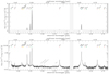 |
Fig. 1. Integrated spectrum extracted from the central three by three spaxels in the wavelength range 2.86 μm < λ < 4.85 μm with flux in linear scale (top) and log scale (bottom). Several emission lines are present and indicated by vertical lines at the top of the panels. We detected seven He I lines, He IIλ4686, Hβ, [O III]λλ4959, 5007, Hα, [N II]λλ6548, 6583, and [S II]λλ6716, 6731. We also report the detection of [Ar IV]λ4711, [Ar IV]λ4740, and [Ar III]λ7136. (We note that [Ar IV]λ4711 is blended with He Iλ4713.) The auroral line [O III]λ4363 is only partly covered by the spectral band of our observation with the G395H grating. The line [O I]λ6003 falls into the detector gap masked here in the region 4.06 μm < λ < 4.14 μm. The BLR components are present in Hβ, Hα, He II, and in the He I lines. In addition, an outflow component is present and is best visible in the broadened asymmetric line base of the [O III] doublet. In the bottom panel, we indicate with grey dotted vertical lines the positions of possible coronal lines, [Fe XVI], [Ca V], [Fe XIII], [Fe V]; of an auroral line, [N II]λ5755; and of another line at λ ∼ 7167.5 Å, the position of which is consistent with Si I. |
Several emission lines are present in the G395H spectrum. We note the prominent, very broad component in all permitted lines in the spectrum: Hβ, Hα, He II, and seven He I lines. These broad components of the permitted lines, and the fact that they are not present in the forbidden lines, unambiguously reveal the presence of a broad line region (BLR) around an accreting black hole. The fact that these lines are significantly fainter than their narrow counterparts implies a type 1.8 classification of this AGN (e.g. Blandford et al. 1990; Whittle 1992). We report the detection of high ionisation [Ar IV] and [Ar III]. With grey dotted vertical lines, we indicate the theoretical positions of several coronal lines, of the auroral line [N II]λ5755, and of another emission line at λ ∼ 7167.5 Å, potentially Si I.
In addition, the base of the [O III] doublet reveals the presence of a slightly redshifted broad wing (though much narrower than the BLR permitted components), which we assume traces a galactic outflow. For a clearer distinction from the BLR and narrow line components, we call this broad wing the ‘outflow’ component.
3.2. Fitting of the integrated G395H spectrum
We fit the full spectrum shown in Fig. 1. We included a narrow line component tracing the emission from the host galaxy (both from the narrow line region and any SF) for all lines, a broader line component tracing the outflow emission for all lines, and a BLR component for the hydrogen and helium lines tracing the high-density gas in the BLR of the AGN. We estimated the continuum through a first-order polynomial, independently for the two spectral regions separated by the detector gap around 4.1 μm. For the full fit, we tied the relative velocities for all narrow and BLR lines together, and we fixed the velocity of the outflow components relative to the narrow components. The velocity widths of all BLR components were tied, assuming that these emission components originate from the same region. We note that this is likely a simplification, as different species may be stratified in the BLR (Peterson & Wandel 1999), but this approach allowed us to better model the BLR components of the faint helium lines. For the narrow and outflow lines, we tied the velocity widths separately around Hα and around [O III]. This allowed us to account in the first approximation for the different spectral resolutions around these main line complexes while still constraining, where possible, the different components of fainter emission lines. We also performed fits tying the line widths in velocity and specifically taking into account the linearly wavelength-dependent spectral resolution of the G395H grating. Overall, this gave very similar results in terms of black hole mass estimates and narrow line ratios; however, we clearly achieved a better fit to the narrow [N II]λ6584 emission than with our fiducial approach. The line widths of the outflow components were affected the most by this choice (see Table 1).
The fit was further constrained through atomic physics (e.g. Osterbrock & Ferland 2006). Thus, the intensity ratio of the [O III] doublet was fixed to [O III]λ5007/[O III]λ4959 = 2.98, and the intensity ratio of the [N II] doublet was fixed to [N II]λ6584/[N II]λ6548 = 2.94. We verified that the [S II] and [Ar IV] doublet ratios were within the physically allowed ranges of 0.44< [S II]λ6716/[S II]λ6731 < 1.45 and 0.12< [Ar IV]λ4711/[Ar IV]λ4740 < 1.37 (for Te = 104 K; see Proxauf et al. 2014, for [Ar IV]). We show a zoom-in of our best fit in Fig. 2. Narrow, outflow, and BLR lines are indicated in green, orange, and purple, respectively, and the full fit is shown in blue.
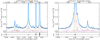 |
Fig. 2. Zoom-in of the integrated spectrum extracted from the central three by three spaxels including our best fit (blue) with individual components for the emission lines (narrow: green, outflow: orange, BLR: purple) for different wavelength ranges. Left panel: Wavelength range including He IIλ4686, [Ar IV]λ4711, He Iλ4713, [Ar IV]λ4740, Hβ, He Iλ4922, [O III]λ4959, and [O III]λ5007. Right panel: Wavelength range including [N II]λ6548, Hα, [N II]λ6584, He Iλ6678, [S II]λ6716, and [S II]λ6731. The bottom sections of each panel show the residuals, res. = data – best fit. We note that for some of the weaker lines, no BLR or outflow component was preferred by the fit. We further note a faint flux excess red-wards of [O III]λ5007 that is undetected in individual spaxels, potentially suggesting some higher velocity (nuclear) outflow components not captured by our fiducial fit. |
We report the emission line properties as constrained from our best fit and used in Sects. 4 and 5 in Table 1. In addition, we briefly discuss the line fluxes of He I in Appendix B. In Sect. 4.1, we use the BLR components to measure the central black hole mass and the outflow line components to constrain outflow properties in Sect. 4.3. In our discussion of line ratio diagnostics in Sects. 5.1 and 5.2, we quote values based on narrow and outflow line components.
3.3. Kinematic maps
We derived maps of projected flux, velocity, and velocity dispersion for the narrow [O III] and Hα lines and for the outflow component as traced by [O III] from multi-component Gaussian fits to the continuum-subtracted emission. Specifically, to derive the 2D maps, we fit the emission in each spaxel separately around [O III] and around Hα. We used two components for [O III]: one for the narrow line emission and one for the broader component that we interpret as an outflow. The amplitude, width, and line centroid of both components were free to vary in these fits. For the fit of the Hα complex, we also used two components: one for the narrow line emission and one for the BLR emission. While we fixed the line centroid of the BLR emission to the narrow line emission, the amplitude and width of both components were free to vary. This simplified approach (i.e. without explicitly accounting for an outflow component or [N II] emission around Hα) allowed us to fit the lower S/N spectra from individual spaxels and, in particular, at larger distances from the source centre. However, we emphasise that the narrow Hα centroid and width are still well constrained due to the outflow and BLR emission being much fainter. We visually inspected the fits to each spaxel and created masks accordingly. The resulting maps are shown in Fig. 3.
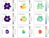 |
Fig. 3. Projected maps of line flux, velocity, and velocity dispersion. Top and middle row: flux (left), velocity (middle), and velocity dispersion corrected for instrumental resolution (right) as measured from the narrow [O III] component (top) and the narrow Hα component (middle) tracing the host galaxy kinematics. Bottom: flux (left), V10, the velocity at the 10th percentile of the emission-line profile (middle), and V90, the velocity at the 90th percentile (right), from the outflow [O III] component. North is up and East is to the left. The spaxel size is 0.1″. A bar in the first column indicates 1″, corresponding to roughly 6 kpc at the source redshift. The highest projected velocities are found in the East-South-East region in both the narrow Hα and [O III] velocity maps, and are possibly related to an ongoing interaction with a faint companion (see Appendix A). Apart from this region, a velocity gradient of Δv ∼ 70 km s−1 along the North-North-West to South-South-East direction is visible in both the narrow [O III] and Hα, possibly indicative of rotation. There is a small offset between the integrated [O III] and Hα line centroids of about 8 km s−1. We find elevated velocity dispersions in the galaxy centre, as expected for observations of a rotating disc affected by beam smearing. The outflow is visible in the nuclear region, with positive and negative velocities respectively the systemic velocity of |600–700| km s−1. |
A velocity gradient of Δv ∼ 70 km s−1 roughly along the north-south direction was visible in both the narrow [O III] and Hα components, which may be interpreted as evidence of rotation. There is a small offset between the integrated [O III] and Hα line centroids of about 8 km s−1, which is much lower than the spectral resolution of our data. We note that we found a kinematic position angle of about PAkin ∼ −15° perpendicular to the morphological PA = 75° (see Sect. 2.1). However, we also note that this compact source is barely resolved in the combined cube with 0.1″ pixel scale, as indicated by the PSF intensity profile imprinted on our line maps (see Fig. 3).
When going to a smaller plate scale and bluer wavelengths in the R100 data, we did see some evidence for structure in the main galaxy, and possibly even for two faint companions (see Appendix A). There is a region of higher positive velocities visible in both the Hα and [O III] maps in the east-south-east direction. It is conceivable that this kinematic feature is related to one of these faint tentative companion galaxies.
The velocity dispersion maps are relatively featureless, but we observed elevated dispersions in the central region of the galaxy in both the Hα and [O III] maps. This is expected for the observed kinematics of a rotating disc that are affected by beam smearing, particularly in the centre. We did not see an increase in dispersion towards the region of higher velocities in the east-south-east.
We observed an outflow in the nuclear region. Positive and negative velocities measured from V10 and V90 range up to |600–700| km s−1 (with respect to the systemic velocity of the galaxy; see bottom-middle and bottom-right panels in Fig. 3).
4. Results
The physical properties derived from our best fit to the fiducial spectrum integrated over the central three by three spaxels are reported in Table 2. We describe our measurements in the following subsections.
4.1. Black hole properties
We found a Hα/Hβ flux ratio of 3.87 ± 0.22 for the BLR components. For quasi-stellar objects (QSOs), intrinsic Hα/Hβ ratios of 3 − 10 are routinely observed (e.g. Osterbrock 1977, 1981), and therefore no correction for extinction was performed. If the BLR Hα luminosity were underestimated due to the presence of dust, the black hole mass calculated in the following paragraph would correspond to a lower limit.
Assuming that the gas in the BLR is virialised, we calculated the central black hole mass from the spectral properties of the Hα BLR region following the calibration by Reines et al. (2013)3:
 (1)
(1)
(their Eq. (5); see also Greene & Ho 2005), where ϵ is a scaling factor dependent on the structure, kinematics, and orientation of the BLR (of the order of ∼1) and reported in the range 0.75 − 1.4 (Onken et al. 2004; Reines et al. 2013). Following Reines & Volonteri (2015), we therefore assumed ϵ = 1.075 ± 0.325. The luminosity LHα and FWHMHα and their uncertainties were measured from our best fit BLR component. In addition, we accounted for the statistical uncertainty of ϵ as based on local MBH − σ⋆ relations by adding 0.4 dex in quadrature to our error budget (e.g. Ho & Kim 2014), which dominates the uncertainty. We measured a black hole mass of log(MBH/M⊙) = 8.2 ± 0.4 (see Table 2).
We verified that using a larger aperture (while constraining the BLR width to the best fit from the fiducial higher S/N spectrum) does not significantly change our results on the black hole mass. By integrating the spectrum over the central 1.15″, we found log(MBH/M⊙) = 8.3 ± 0.4. This result indicates that the BLR emission is nearly fully encompassed by the central three by three spaxels.
Alternatively, by using the calibrations by Greene & Ho (2005) that utilise the Hα BLR emission, the Hβ BLR emission, and the L5100 luminosity and by again accounting for the scatter of the local virial relations, we found log(MBH/M⊙) = 8.0 ± 0.4, log(MBH/M⊙) = 7.9 ± 0.4 and log(MBH/M⊙) = 8.2 ± 0.4, respectively. These estimates are consistent with the estimate using the calibration by Reines et al. (2013).
We used different calibrations to estimate the bolometric luminosity Lbol of GS_30734. First, assuming that the narrow line emission is dominated by the AGN, we calculated the Lbol from the narrow line luminosities of Hβ and [O III] following Eq. (1) by Netzer (2009). This gave log(Lbol/(erg s−1)) = 46.2 and likely represents an upper limit. When we used Eq. (25) by Dalla Bontà et al. (2020) to estimate Lbol from the Hβ BLR luminosity, we got log(Lbol/(erg s−1)) = 45.3. We found a similar value, namely, log(Lbol/(erg s−1)) = 45.2 ± 0.4, when calculating Lbol using Eq. (6) by Stern & Laor (2012) and utilising the Hα BLR luminosity.
Based on our black hole mass estimate from the Hα BLR (Eq. (1)), the Eddington luminosity is log(LEdd/(erg s−1)) = 4πGMBHmpc/σT = 46.3 ± 0.4, where G is the gravitational constant, mp the proton mass, c the speed of light, and cT the Thomson scattering cross-section. Depending on which bolometric luminosity and which black hole mass estimate we adopted, we found Eddington ratios in the range of λEdd = Lbol/LEdd = 0.1 − 1.6 (see Table 2).
4.2. Host galaxy dynamical mass
In our IFU observations, GS_3073 is very compact and barely resolved (see also discussion by Vanzella et al. 2010). We estimated its dynamical mass by means of the integrated narrow component line width (corrected for instrumental broadening) as follows:
 (2)
(2)
where K(n) = 8.87 − 0.831n + 0.0241n2, with the Sérsic index as n following Cappellari et al. (2006); K(q) = [0.87 + 0.38e−3.71(1 − q)]2, with the axis ratio as q following van der Wel et al. (2022); and Re as the effective radius. In this calibration, σ is the integrated stellar velocity dispersion. Bezanson et al. (2018) have shown that galaxies with low integrated ionised gas velocity dispersion tend to have higher integrated stellar velocity dispersion (their Fig. 4b). We took this into account by applying a correction of Δlog(σ/(km s−1)) = +0.1 to our measured narrow line dispersion (σHα, narrow = 83 km s−1).
When adopting the structural parameters n = 8, q = 0.71, and Re = 0.18 kpc from Sérsic fits to the H-band photometry by van der Wel et al. (2012), we found log(Mdyn/M⊙)∼9.2. Since a Sérsic index of n = 8 is at the edge of the explored parameter space in the fits by van der Wel et al. (2012), and likely biased by the presence of the AGN at the centre of the galaxy, we adopted n = 4 to derive a fiducial dynamical mass, leading to log(Mdyn/M⊙)∼9.4. We found similar values when we adopted the calibration between inclination-corrected integrated line widths and disc velocities by Wisnioski et al. (2018) together with their Eq. (3), namely, log(Mdyn/M⊙)∼8.9, as well as when we attempted to replace the integrated ionised gas velocity dispersion with  , namely, log(Mdyn/M⊙)∼9.3, where vobs is half the inclination-corrected maximum observed velocity gradient and σobs is the average observed velocity dispersion of individual spaxels in the outer region of the galaxy (both uncorrected for beam smearing; see Fig. 3). A large uncertainty in these calculations stems from the structural parameters of GS_3073. Overall, if we vary the size between 0.11 and 0.9 kpc, we find dynamical mass estimates in the range of 9.2 < log(Mdyn/M⊙) < 10.1 (see Table 2), and if we also vary the Sérsic index between 0.5 and 8 (see values reported by Vanzella et al. 2010), we find estimates in the range of 9.0 < log(Mdyn/M⊙) < 10.3.
We note that previous estimates in the literature of the total stellar mass from SED fitting for GS_3073 are larger than our dynamical mass estimate, with the most recent estimate being log(M⋆/M⊙)∼10.6 (Barchiesi et al. 2023). These estimates are based on broadband photometry that had unknown emission line contributions. We found strong emission lines that would significantly contaminate the 3.6 and 4.5 μm Spitzer Infra-Red Array Camera (IRAC) fluxes, which are the rest-frame optical constraints closest to the Balmer-break region and therefore most important for stellar mass estimates. If not accounted for properly, these emission lines could lead to overestimates of the stellar mass. We used the R100 spectrum to provide an updated stellar mass estimate based on the continuum emission. We observed no strong Balmer-break in the spectrum, and cannot rule out significant contribution or even dominance of the continuum light from the accretion disc surrounding the black hole. Under the assumption that the continuum light is dominated by the host galaxy, we fit the continuum in the region 2.73 − 5.30 μm using BEAGLE (Chevallard & Charlot 2016) while fully masking the emission lines (which have multiple physical contributions). Using a constant star formation history (SFH), we found a stellar mass estimate of log(M⋆/M⊙)∼9.52 ± 0.13, where the uncertainties denote the 1σ credible interval. We found a similar stellar mass estimate when fitting the full spectrum (rest-frame UV to optical) with a delayed SFH, where the last 10 Myr were replaced with a constant SFR which was allowed to vary. This estimate is consistent within the uncertainties of our dynamical mass estimate, and we used it as a fiducial value for the stellar mass of GS_3073.
In Fig. 4, we compare our black hole mass measurement as a function of host galaxy stellar mass and host galaxy dynamical mass to that of various literature compilations and relations derived locally and at high redshift. Reines & Volonteri (2015) provide a compilation of local AGN for which the black hole mass has been measured from Hα BLR components with the same calibration that we use for our MBH measurement. In addition, some local data points come from reverberation mapping. The black hole of GS_3073 is more massive by more than two orders of magnitude compared to the best fit relation of the local sample and more massive than all local broad line AGN by Reines & Volonteri (2015). In the figure, we also show two data points from Kocevski et al. (2023) at z ∼ 5.2 and z ∼ 5.6 (see also Onoue et al. 2023). For consistency with our measurement and the z = 0 data, we recalculated the black hole masses based on Eq. (1). This recalibration resulted in an increase of the black hole mass by ∼0.2 dex relative to what is quoted by the authors. (Following the discussion in that paper, we assumed AV = 4 for the higher mass source.) These two sources appear more consistent with the local BLR population, but since their stellar mass estimates are upper limits, these black holes could also be overly massive.
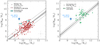 |
Fig. 4. Central black hole mass MBH as a function of host galaxy stellar mass Mstar (left) and host galaxy dynamical mass Mdyn (right) for GS_3073 (blue filled star) and literature compilations. Left panel: Comparison of our galaxy to local AGN by Reines & Volonteri (2015). In this case, the black hole mass was determined from a BLR or from reverberation mapping (red circles, with representative error bar in grey). The black line with a shaded region shows the best fit with uncertainties to this data by Reines & Volonteri (2015), and the dashed lines indicate the intrinsic scatter plus measurement uncertainties. As teal diamonds, we show data by Kocevski et al. (2023) for which we calculated the black hole mass based on Eq. (1) for consistency with our measurement and the z = 0 data. Right panel: Comparison of our galaxy to z ≥ 6 QSOs by Izumi et al. (2021, green diamonds). For our dynamical mass estimate, we adopted a Sérsic index of nS = 4 and an effective radius of Re = 0.18 kpc. We indicated uncertainties by varying Re between 0.11 and 0.9 kpc. The black line shows the local MBH − Mbulge relation with uncertainties and intrinsic scatter by Kormendy & Ho (2013). The black hole of GS_3073 is at the lower end of the MBH − Mdyn distribution when compared to the measurements by Izumi et al. (2021), but it still appears overly massive for its host galaxy’s dynamical mass when compared to the local relation by Kormendy & Ho (2013). Considering the MBH − Mstar relation, the black hole of GS_3073 is much more massive in comparison to local broad line AGN with a similar host galaxy stellar mass. |
At high redshift, existing black hole mass measurements are primarily obtained from luminous quasars (QSOs; log(Lbol/(erg s−1)) ∼ 46.5 − 48) for which stellar mass estimates are not available. In the right panel of Fig. 4, we compare the black hole mass of GS_3073 as a function of host galaxy dynamical mass to z ≥ 6 QSOs compiled by Izumi et al. (2021, see also their Fig. 13), which includes data by Willott et al. (2010), De Rosa et al. (2014), Kashikawa et al. (2015), Venemans et al. (2015), Bañados et al. (2016), Jiang et al. (2016), Shao et al. (2017), Mazzucchelli et al. (2017), Decarli et al. (2018). Our galaxy sits at the lower end of the QSO MBH distribution (see also the compilations by Willott et al. 2017; Pensabene et al. 2020). Similar to several of the measurements compiled by Izumi et al. (2021), GS_3073 appears to sit above the local MBH − Mbulge relation constrained by Kormendy & Ho (2013). However, we note that the comparison of the high−z dynamical mass measurements to the local bulge mass measurements constrained from elliptical and S/S0 galaxies is not straightforward. As discussed by Reines & Volonteri (2015), even when accounting for differences in assumptions about the initial mass function and when assuming that the bulge dynamical mass corresponds to the total stellar mass, the slope and normalisation of the z = 0 relations differ (see also discussion by Kormendy & Ho 2013).
4.3. Outflow properties based on the integrated spectrum
Faint but clearly detected wings different from the BLR are seen in most of the strong emission lines in the integrated spectrum extracted from the central three by three spaxel of GS_3073 (see Fig. 2), which we interpret as tracing an outflow (in line with other outflow indications by Vanzella et al. 2010; Grazian et al. 2020). The outflow emission appears almost symmetric but slightly redshifted, suggesting that the majority of the outflow is pointing away from the observer (see also Vanzella et al. 2010; Grazian et al. 2020). We measured the maximum projected outflow velocity as vout = ⟨voutflow⟩+2σoutflow, where σoutflow is corrected for instrumental resolution (e.g. Genzel et al. 2011; Davies et al. 2019). At the position of [O III], we measured vout = 1211 ± 20 km s−1, while at the position of Hα, we measured vout = 685 ± 11 km s−1 (see description of fitting model in Sect. 3.2). At the [O III] position, we noted an even more extended, faint redshifted wing in emission that is not captured by our best fit model (see left panel of Fig. 2). The velocity separation of this emission reaches roughly 3100 km s−1, suggesting a more complex and vigorous outflow5.
For the calculation of outflow properties, such as the mass outflow rate Ṁout,ion and mass loading factor ηion = Ṁout,ion/SFR, we used our measurements from the Hα outflow component, but we note that they may correspond to lower limits given the higher velocity emission seen for the [O III] outflow. We adopted a simple model to estimate Ṁout,ion from the Hα outflow component, assuming a photo-ionised constant velocity (vout) spherical outflow of extent Rout, following Genzel et al. (2011), Newman et al. (2012), Förster Schreiber et al. (2019), Davies et al. (2019, 2020), Cresci et al. (2023):
 (3)
(3)
where 1.36 mH is the effective nucleon mass for a 10 percent helium fraction, γHα = 3.56 × 10⁻²⁵ erg cm−3 s−1 is the Hα emissivity at T = 104 K, ne, outflow is the electron density in the outflow, and LHα, outflow is the Hα luminosity of the outflow component.
The [S II] lines are comparatively weak for GS_3073, and no outflow line component in the [S II] doublet was preferred by our best fit. From the narrow component fit, we inferred F[S II]λ6716/F[S II]λ6731 = 0.69 ± 0.28, which corresponds to an electron density of ne,[S II] ∼ 1869 cm−3 for T = 104 K, using the calibration by Sanders et al. (2016). Alternatively, we could measure the electron density in the narrow and outflow component also from the [Ar IV]λλ4711, 4740 ratio (e.g. Proxauf et al. 2014). However, in our case, the [Ar IV]λ4711 line is blended with He Iλ4713, making this measurement uncertain (see Fig. 2). Though we could not easily constrain the outflow component ratio, we report a density of ne,[Ar IV] = 3032 cm−3 based on the narrow component ratio, which is in line with this emission originating from higher density regions.
For the density of the outflow component, since this is unconstrained by our data, we followed Förster Schreiber et al. (2019) in assuming ne, outflow = 1000 cm−3 (i.e. their fiducial value for AGN-driven outflows; see also e.g. Perna et al. 2017; Kakkad et al. 2018). With LHα, outflow = 12.4 × 1042 erg s−1 and adopting Rout = Re ∼ 0.18 kpc, we found Ṁout,ion ∼ 98 ± 2 M⊙ yr−1. This is comparable to AGN with strong ionised outflows at 1 < z < 3 (Förster Schreiber et al. 2019). It is reasonable to assume that the total mass loss due to outflows is larger since we are only probing the warm ionised gas phase with our measurements. Rupke et al. (2017) and Fluetsch et al. (2019) studied the relation between MBH and Ṁout from various gas phases in local galaxies. For GS_3073 we found a mass outflow rate that is about twice as high as their best fit relations but nevertheless well within the spread of individual measurements.
We further estimated the mass loading factor ηion = Ṁout,ion/SFR. The SFR estimates in the literature from SED fitting for GS_3073 vary and are in the range of SFR ∼ 30 − 410 M⊙ yr−1 (Barro et al. 2019; Faisst et al. 2020). From the [C II]λ158 μm luminosity, Barchiesi et al. (2023) derived ![Mathematical equation: $ \mathrm{SFR}_{\mathrm{[CII]}}=16^{+14}_{-7}\,M_\odot $](/articles/aa/full_html/2023/09/aa46137-23/aa46137-23-eq9.gif) yr−1. Since the Hα narrow line flux likely has a strong AGN contribution, we instead used the SFR[CII]6. From this we derived
yr−1. Since the Hα narrow line flux likely has a strong AGN contribution, we instead used the SFR[CII]6. From this we derived  . This result suggests the AGN in GS_3073 is powerful enough to expel more mass from the galaxy than is currently consumed by SF, particularly when considering the addition of cold and hot gas likely entrenched in the outflow. We caution that the estimates of both Ṁout,ion and ηion are uncertain due to the substantial uncertainties regarding the ionised gas density and outflow geometry.
4.4. Electron temperature and metallicity
Our observations cover part of the auroral [O III]λ4363 emission line, which can be used in conjunction with [O III]λλ4959, 5007 to measure the electron temperature and gas phase metallicity (e.g. Izotov et al. 2006; Curti et al. 2017 and Maiolino & Mannucci 2019 for a review). Although [O III]λ4363 is only partly covered in our R2700 data, we could still perform a simultaneous fit with the other emission lines in our spectrum by fixing the relative line position and the line widths to [O III]λ5007. While tentative, this gives an electron temperature of  K based on the narrow line ratio [O III]λ4363/[O III]λλ4959, 5007. For this calculation, we assumed an electron density of 103 cm−3, which is consistent within the uncertainties of our best fit value based on the [S II] doublet and corresponds to the same value we adopted for the calculations of the outflow properties (Sect. 4.3). We note however that Te, [OIII] (i.e. the electron temperature of the high ionisation zone) is relatively insensitive to the exact value of the electron density within a range of 102 − 104 cm−3. Following Dors et al. (2020), we assumed that the narrow line emission is dominated by AGN excitation and found that the measured Te corresponds to a metallicity of about 0.2 Z⊙, or 12 + log(O++/H)
 -pagination 7. By itself, this corresponds to a lower limit due to the unknown contribution of the other ionic species to the total oxygen abundance.
In our R100 observations of GS_3073, we covered the wavelength range of λ = 0.6 − 5.3 μm, which includes the [O II]λλ3727, 3730 doublet (see Appendix C). Together with our R2700 data8, this allowed us to constrain the full O/H abundance. We measured the [O II]λλ3727, 3730 flux from an aperture that gives [O III]λλ4959, 5007 flux consistent within 3 percent of our measurement from the R2700 data. We found the contribution from O+/H to be minor. Exploiting the [O II]λλ3727, 3730 flux and following the prescriptions from Dors et al. (2020) to account for the temperature of the low ionisation region in Seyfert galaxies, we derived a total oxygen abundance of 12 + log(O/H) , corresponding to
  percent solar metallicity. We note that the contribution to the total abundance from even higher ionisation states of oxygen is expected to be fully negligible, as the ionisation correction factor (ICF) computed on the basis of the He+ and He++ abundances is ICF(O) = N(He++He++)/N(He+) = 1.017 (Torres-Peimbert & Peimbert 1977; Izotov et al. 1994). As shown in Fig. 5, this places our galaxy well below the gas-phase mass-metallicity relations measured from z = 0 to z ∼ 3 (Curti et al. 2020b; Sanders et al. 2021) and in line with the relation inferred for star-forming galaxies at 4 < z < 10 by Nakajima et al. (2023).
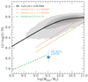 |
Fig. 5. GS_3073 in the mass-metallicity plane (blue star). The z ∼ 0.08 relation based on SDSS data by Curti et al. (2020a) is shown as grey shading with the best fit in black. The red and yellow dash-dotted lines show the best fit relations at z ∼ 2.3 and z ∼ 3.3, respectively, by Sanders et al. (2021) based on data from the MOSDEF survey (Kriek et al. 2015). The dashed green line shows the best fit relation obtained by Nakajima et al. (2023) based on a compilation of early JWST data at redshifts 4 < z < 10. At z = 5.55, GS_3073 is slightly more massive but still compatible with the extrapolation of this relation. |
5. Discussion
5.1. An AGN in the SFG regime of the classical line ratio diagnostic diagrams
An important result of our work is that low metallicities in the early Universe blur the differences in classical diagnostic line ratios between galaxies that are primarily ionised by SF versus AGN activity. This can be appreciated in Fig. 6, where we depict the placement of our galaxy in the line ratio diagnostic diagrams showing [O III]/Hβ versus [N II]/Hα (left; Baldwin et al. 1981) and [O III]/Hβ versus [S II]λλ6717,6731/Hα (right; Veilleux & Osterbrock 1987). Our source (green, purple, and blue filled stars for narrow, outflow, and narrow+outflow line ratios, respectively) has an [N II]/Hα ratio that is lower than the majority of local SFGs and well separated from the local AGN branch. The [N II]/Hα and [S II]/Hα narrow line ratios of GS_3073 are also much lower than those of massive SFGs at 1 < z < 3, while the [O III]/Hβ ratio is above average (e.g. Steidel et al. 2014; Strom et al. 2017; Curti et al. 2020a; Topping et al. 2020; see Maiolino & Mannucci 2019 for a review). Despite being an AGN, the low [N II]/Hα and [S II]/Hα line ratios place our source in the star-forming regime of the classical z = 0 line ratio diagnostic diagrams.
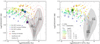 |
Fig. 6. Diagnostic diagrams of [O III]λ5007/Hβ versus [N II]λ6584/Hα (left) and [O III]λ5007/Hβ versus [S II]λλ6717,6731/Hα (right). The position of GS_3073 is indicated with the green, purple, and blue filled stars as constrained by its narrow, outflow, and narrow+outflow line ratios, respectively. Local galaxies from SDSS (Abazajian et al. 2009) are indicated by the grey shading, with the contours encompassing 98, 80, and 50 percent of the sample. The red contours encompass 95, 80, and 50 percent of SDSS broad line AGN as classified by Hviding et al. (2022). The dashed line indicates the demarcation by Kauffmann et al. (2003) between galaxies primarily ionised by SF (left) and AGN (right). The dotted lines by Kewley et al. (2001) include more extreme starbursts or composite objects among the star-forming galaxies to the left. The thin coloured symbols (stars, crosses, triangles) show model grids for AGN and direct collapse black holes by Nakajima & Maiolino (2022) for an accretion disc temperature of Tbb = 2 × 10⁵ K, power law indices constraining the slope between the optical and X-ray bands (α = −1.2, −1.6, −2.0, corresponding to stars, crosses, triangles), ionisation parameters (−3.0 < log U < −0.5, indicated by increasing symbol size), and gas phase metallicities (Zgas = 0.001 − 0.028, teal to red colours). A gas density of 103 cm−3 was assumed. Grey symbols show models with lower Tbb. The open circles show model grids for galaxies using BPASS SEDs (Eldridge et al. 2017; Stanway & Eldridge 2018), with binary evolution based on a Kroupa (2001) initial mass function with an upper mass cut of 300 M⊙ and a stellar age of 10 Myr (see Nakajima & Maiolino 2022 for details). Here, the dark to light colours indicate stellar metallicities in the range Z⋆ = 0.0006 − 0.0084. Compared to these theoretical models, GS_3073 has line ratios compatible with being either a low-metallicity AGN or a low-metallicity SFG, despite being located within the classical SFG regime in the diagrams. |
Theoretical models have predicted that AGN in the early Universe might populate the ‘star-forming’ regime of the classical line ratio diagnostics, to the left of the z = 0 AGN branch, mainly due to their lower metallicities. This is shown in Fig. 6 with thin stars, crosses, and triangles, which represent model predictions by Nakajima & Maiolino (2022) for AGNs with varying metallicities, ionisation parameters, and power law indices (see also e.g. Groves et al. 2006; Kewley et al. 2013a; Feltre et al. 2016; Gutkin et al. 2016; Hirschmann et al. 2017, 2019; and see Hirschmann et al. 2022 for a study of post-processing cosmological simulations). Models with an accretion disc temperature of Tbb = 2 × 10⁵ K are shown with coloured symbols, while models with Tbb = 5 × 10⁴ K and Tbb = 1 × 10⁵ K are shown as grey symbols.
If we consider theoretical model predictions for early galaxies with massive stars, indicated by blue and purple circles in Fig. 6, they are also in agreement with the location of GS_3073. These models suggest that the classical line ratio diagnostic diagrams alone cannot be used to distinguish SFGs and AGN in the early Universe. Our data demonstrate that high−z AGN can indeed populate the ‘star-forming’ regime of the classical line ratio diagnostics (see also Kocevski et al. 2023).
We note that some low-metallicity, low−z AGN were also found in the star-forming region of the classical line ratio diagnostic diagrams, although typically with higher [N II]/Hα ratios (> 0.1) than our source (but see also e.g. Simmonds et al. 2016; Cann et al. 2020; Burke et al. 2021). This can be appreciated through the location of z ≲ 0.3 AGN with broad Balmer lines by Hviding et al. (2022), indicated with red contours in the left panel of Fig. 6 (see also e.g. Shirazi & Brinchmann 2012; Kawasaki et al. 2017; Keel et al. 2019).
Since we knew that GS_3073 is an AGN and we had an estimate of its gas phase metallicity from the narrow line ratios (Sect. 4.4), we used this information together with the theoretical model predictions to further constrain the ionisation parameter, U, and the power law index of the energy slope between the optical and X-ray bands, α. Based on our measurement of Zgas/Z⊙ = 0.21, we focussed on models with Zgas = 0.0028 (20 percent solar; yellow-green symbols by Nakajima & Maiolino 2022 in Fig. 6) in the BPT diagram (left panel) in which our measured line ratios have the highest S/N. We found that our BPT narrow line ratios are consistent with log(U) = − 2.0 and α = −1.2.
5.2. Using He IIλ4686 to discriminate SFGs from AGN
To account for the unique conditions in the early Universe, alternative diagnostic diagrams have been proposed to separate SFGs from AGN. Several of them rely on the properties of the He IIλ4686 emission we also detected in our galaxy9 (e.g. Shirazi & Brinchmann 2012; Bär et al. 2017; Nakajima & Maiolino 2022).
In Fig. 7, we show the placement of our source in two diagnostic diagrams utilising He IIλ4686. In the left panel, we show the equivalent width EW(He IIλ4686) as a function of He IIλ4686/Hβ. This diagram provides constraints on the shape of the ionising spectrum and the temperature of the accretion disc. The presence of He IIλ4686 with an ionisation potential of 54.4 eV requires sources of hard ionising radiation. Its equivalent width increases with an increasing fraction of highly ionising photons over non-ionising photons and has therefore been promoted as an indicator of Population III stars (their proposed location is indicated in Fig. 7 by the dotted grey box). He IIλ4686/Hβ effectively constrains the shape of the ionising spectrum through the ratio of ionising photons with E > 54.4 eV to E > 13.6 eV.
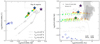 |
Fig. 7. Diagnostic diagrams of EW(He IIλ4686) versus He IIλ4686/Hβ(left) and He IIλ4686/Hβ versus [N II]λ6584/Hα (right). The symbols are the same as in Fig. 6: Thin stars, crosses, and triangles show evolved AGN and direct collapse black holes; circles show evolved SFGs; and the position of GS_3073 is indicated by the large, filled stars (green: narrow, blue: narrow+outflow, purple: outflow). In the left panel, lines of constant Tbb = 5 × 10⁴ K, 1 × 10⁵ K, 2 × 10⁵ K correspond to dashed, dash-triple-dotted, and dash-dotted lines. In the left panel, the dotted region in the top right indicates the regime expected for Pop III stars. In the right panel, narrow line ratios from local He II-selected AGN by Tozzi et al. (2023) are indicated by the grey shading with contours encompassing 94, 80, and 50 percent of the sample. The dotted line indicates the demarcation by Shirazi & Brinchmann (2012) separating SFGs (left) from AGN (right) at z = 0. In the EW(He IIλ4686) versus He IIλ4686/Hβ diagram, GS_3073 is compatible with an AGN with a hot accretion disc and is clearly separated from SFGs. This is also the case for the He IIλ4686/Hβ versus [N II]λ6584/Hα diagnostic (right), although the locally constrained demarcation line by Shirazi & Brinchmann (2012) appears to evolve with redshift if we consider the location of the model predictions, particularly for AGNs with α = −2.0 (thin triangles). |
The location of GS_3073 (green, purple, and blue filled stars for the narrow, outflow, narrow+outflow line ratios) in this diagram is better reproduced by models using the high accretion disc temperature of Tbb = 2 × 10⁵ K (symbols connected by the dash-dotted line), possibly indicating an even higher temperature. Notably, a high temperature of the accretion disc is generally associated with smaller black holes. Such a characteristic for this AGN would be in line with the fact that its black hole is smaller than most black holes inferred for more luminous quasars at similar redshift. Both the high equivalent width of He IIλ4686 and the high He IIλ4686/Hβ ratio clearly separate our galaxy from model predictions of galaxies without an AGN (blue and purple circles).
The situation is similar for the line ratio diagnostic in the right panel of Fig. 7, which was originally suggested by Shirazi & Brinchmann (2012) to more clearly distinguish sources primarily ionised by SF versus AGN in the local Universe. In this figure, we also show as grey shading z = 0 data by Tozzi et al. (2023), who selected AGN-dominated spaxels (with > 50% of He IIλ4686 flux excited by the AGN) from galaxies in the Mapping Nearby Galaxies at Apache Point Observatory (MaNGA) survey (Bundy et al. 2015). We note that the authors subtracted any BLR emission before measuring the line ratios. Similar to the BPT diagram, local He IIλ4686-selected AGN have higher [N II]/Hα ratios compared to GS_3073. Considering the Nakajima & Maiolino (2022) model predictions for early SFGs (circles) and AGN (other small coloured symbols), the separation between SFGs and AGN still prevails at high redshift, even though the demarcation line might evolve over time, as suggested by the placement of the model predictions compared to the z = 0 data.
The classical line ratio diagnostic diagrams could not help in identifying the primary ionisation source for the low-metallicity galaxy GS_3073 (see Sect. 5.1). However, the placement of GS_3073 in the He IIλ4686 diagnostics, which were discussed with respect to theoretical predictions, suggests that those diagnostics can be used instead.
5.3. Massive black holes in the early Universe
Our measurement of log(MBH/M⊙)∼8.2 from the Hα BLR is among the few measured ‘lower mass’ black holes at z > 5 (see also Kocevski et al. 2023). Still, the black hole of GS_3073 appears overly massive compared to local scaling relations by Reines & Volonteri (2015) and Kormendy & Ho (2013) and compared to theoretical model predictions (e.g. Trinca et al. 2023, based on the 2 μm flux; priv. comm.). This finding is similar to other black hole mass measurements at higher redshift.
If black holes at higher redshift are comparatively more massive, this could suggest a more rapid growth of black holes in the early Universe, possibly fuelled by larger gas fractions or more efficient accretion. Higher accretion rates could plausibly be achieved in systems with a higher density. This idea is encapsulated in the analytical model by Chen et al. (2020), where at a fixed stellar mass, smaller SFGs host more massive black holes due to higher central densities. Assuming our fiducial Re = 0.18 kpc and log(M⋆/M⊙) = 9.52, their MBH − Re − Mstar relation (their Eq. C12) predicts a black hole mass of log(MBH/M⊙)∼7.0. This prediction is above the local MBH − Mstar relation (see Fig. 4) and in line with our findings, but it is still lower than our measurement of log(MBH/M⊙)∼8.2.
Interestingly, overly massive black holes are also found in a comparable region of the MBH − M⋆ parameter space in some z ≲ 1 dwarf galaxy AGN (e.g. Burke et al. 2022; Mezcua et al. 2023; Siudek et al. 2023). These galaxies may evolve onto the local Mbulge − MBH relation by z = 0 (Mezcua et al. 2023). Larger black hole masses at earlier times have also been predicted by some cosmological simulations, while others have shown the opposite trend (see Habouzit et al. 2021, 2022). Consolidating a picture of high−z black hole masses in relation to their host galaxy properties over a wide range in masses could therefore serve as a powerful discriminant of feedback implementation.
5.4. AGN feedback and enrichment of the intergalactic medium
Theoretical work suggests that AGN feedback is crucial in quenching galaxies with host galaxy masses close to the Schechter mass (log(Mstar/M⊙) ∼ 11; e.g. Di Matteo et al. 2005; Croton et al. 2006; Bower et al. 2006; Hopkins et al. 2006; Cattaneo et al. 2006; Somerville et al. 2008), and this is supported by observational evidence (e.g. Veilleux et al. 2005; McNamara & Nulsen 2007; Fabian 2012; Genzel et al. 2014; Harrison et al. 2014, 2016; Heckman & Best 2014; Förster Schreiber et al. 2014, 2019). Its impact has also been demonstrated empirically (e.g. Penny et al. 2018; Manzano-King et al. 2019; Mezcua et al. 2019; Liu et al. 2020; Davis et al. 2022) and theoretically (e.g. Koudmani et al. 2019, 2021) for galaxies with much lower masses.
In Fig. 8, we compare the mass outflow rate (left) and kinetic power  (right) measured from the fit to the spectrum of GS_3073 integrated over the central three by three spaxels (Fig. 2, Sect. 4.3) as a function of the AGN bolometric luminosity to local and lower redshift sources (z < 3.5) by Fiore et al. (2017) and to two z ∼ 6.8 QSOs by Marshall et al. (2023). The outflow energetics of GS_3073 are consistent with the scaling derived from the lower−z data, suggesting that the driving mechanisms in z > 5 AGN do not differ strongly from their lower−z counterparts. Interestingly, the kinetic power is only ∼0.1 − 1.0% of the radiative luminosity of the AGN. This is generally considered as an indication of the outflow being rather ineffective at depositing energy into the ISM and therefore providing no major feedback to the galaxy, at least not in the direct ejective mode. As predicted by many theoretical models (e.g. Gabor & Bournaud 2014; Roos et al. 2015; Bower et al. 2017; Nelson et al. 2019; Zinger et al. 2020), while the ionised outflow may have little impact on the ISM (possibly because of poor coupling), it can potentially escape into the circum-galactic medium (CGM). Thus, it may contribute to its heating and hence suppress fresh gas accretion and possibly result in delayed feedback in the form of starvation.
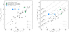 |
Fig. 8. Mass outflow rate Ṁout,ion (left) and kinetic power Pk,ion (right) of the warm ionised gas phase as a function of AGN bolometric luminosity Lbol. The grey circles show ionised gas outflows at 0 < z < 3.5 by Fiore et al. (2017), the green stars show two z ∼ 6.8 QSOs from the GA-IFS GTO programme by Marshall et al. (2023), and the blue stars show the range of bolometric luminosities inferred for GS_3073, as discussed in Sect. 4.1. We have scaled the measurements by Fiore et al. (2017) and Marshall et al. (2023) to correspond to an electron density in the outflow of ne = 1000 cm−3, as assumed in this work. For Lbol, we indicate a representative error bar of 0.5 dex, and for Ṁout,ion and Pk,ion, we indicate how much they would change if ne, Rout, or vout were different by factors 1/5, 5, and 2/3, respectively (see main text for details). The dashed line in the left panel is a linear fit in logarithmic scales to the data by Fiore et al. (2017). The dashed lines in the right panel show constant ratios of Pk and Lbol. The outflow energetics of GS_3073 in relation to the bolometric AGN luminosity are consistent with lower−z scaling relations, suggesting that the driving mechanisms in z > 5 AGN do not differ from their lower−z counterparts. |
We emphasise that the quantities discussed here and shown in Fig. 8 are subject to substantial uncertainties. As mentioned in Sect. 4.3, the unknown electron density of the outflowing material and the uncertain outflow geometry hamper a robust estimate of Ṁout,ion and Pk,ion. As a reference for Ṁout,ion and Pk,ion in Fig. 8, we indicate with arrows how much they would change if ne, Rout, or vout were different by factors 1/5, 5, and 2/3, respectively. Changes in these quantities due to a different definition of the outflow velocity or a different assumption on the gas density or the extent of the outflow dominate the uncertainties (see Sect. 4.3). For the uncertainty on Lbol, we indicate 0.5 dex, which is motivated by the range of values derived for GS_3073 and the estimate by Fiore et al. (2017).
We measured relatively large projected outflow velocities and estimated a high mass loading factor for GS_3073 based on our fit to the integrated spectrum over the central three by three spaxels (Fig. 2, Sect. 4.3). At the same time, we inferred a relatively low dynamical mass for our galaxy (Sect. 4.2). This suggests that indeed a substantial fraction of the material expelled by the outflow could escape the potential well of the galaxy and enrich the CGM and even the intergalactic medium.
To quantify this, we estimated the escape velocity at radius r assuming an isothermal sphere following Arribas et al. (2014) as
![Mathematical equation: $$ \begin{aligned} v_{\rm esc}\approx \sqrt{\frac{2M_{\rm dyn}G [1+\ln (r_{\rm max}/r)]}{3r}}, \end{aligned} $$](/articles/aa/full_html/2023/09/aa46137-23/aa46137-23-eq16.gif) (4)
(4)
where rmax is the truncation or halo radius. Evaluating at r = Re = 0.18 kpc with rmax = 100 r, we found vesc ∼ 490 km s−1. Comparing this to our measured outflow velocity of vout = 685 km s−1, with some material reaching velocities of few 1000 km s−1 as based on the outflow [O III] component, this indicates that a sizeable fraction of the outflowing gas could indeed escape the galaxy’s potential well. From the distribution of outflow velocities in our best fit outflow components, we found that about 10 − 40 percent of the emitting ionised gas has velocities in excess of vesc ∼ 490 km s−1 when considering both the components around Hα and around [O III]. This suggests that at least 10 − 40 M⊙ yr−1 of warm ionised gas could escape the galaxy potential if feedback would sustain the measured outflow velocities and mass outflow rates. This material could thus contribute to metal enrichment of the intergalactic medium at this early time in cosmic history.
We note that this estimate likely represents a lower limit for two reasons: First, the measured outflow velocities are projected (i.e. intrinsic outflow velocities will be even larger). Second, we do not account for gas phases other than warm ionised gas plausibly entrenched in the outflow. In particular, we expect contributions from cold gas (molecular and neutral) that likely dominate the outflow mass budget (see e.g. Rupke & Veilleux 2013; Herrera-Camus et al. 2019; Roberts-Borsani 2020; Fluetsch et al. 2021; Avery et al. 2022; Baron et al. 2022; Cresci et al. 2023).
6. Conclusions and outlook
We have presented deep JWST/NIRSpec-IFS data of the galaxy GS_3073 at z = 5.55. We focussed on the high spectral resolution spectrum (G395H, R ∼ 2700) obtained with 5 h on source, and we also used a shorter exposure (1 h) prism spectrum (R ∼ 100). The high-resolution spectrum revealed about 20 rest-frame optical nebular emission lines, some of which were detected with very high S/N, and another 14 lines/doublets are visible in the prism spectrum. The main results of our analysis are as follows:
-
Permitted lines, such as Hα, Hβ, He I, and He II, are characterised by a broad component (not observed in the forbidden lines) that can be unambiguously interpreted as tracing the BLR around an accreting SMBH and clearly identifying GS_3073 as an AGN (type 1.8).
-
From the narrow line ratios, we measured a gas phase metallicity of Zgas/Z⊙ ∼ 0.21, which is lower than what has been inferred for both more luminous AGN at a similar redshift and lower−z AGN.
-
We empirically showed that classical line ratio diagnostics (Baldwin et al. 1981; Veilleux & Osterbrock 1987) cannot be used to distinguish between the primary ionisation source (AGN or SF) for such low-metallicity systems, whereas different diagnostic diagrams involving He IIλ4686 proved useful.
-
We measured the central black hole mass of GS_3073 to be log(MBH/M⊙)∼8.2. While this places our galaxy at the lower end of known high−z black hole masses, it still appears to be overly massive compared to its host galaxy properties, such as stellar mass or dynamical mass.
-
We detected an outflow with velocity vout = 685 km s−1 and a mass outflow rate of about 100 M⊙ yr−1, suggesting that one billion years after the Big Bang, GS_3073 is able to enrich the intergalactic medium with metals.
Additional JWST data, especially spectroscopic surveys utilising the micro-shutter assembly, will certainly uncover more AGN like the one presented in this paper and will allow an assessment of the AGN and black hole population in the early Universe. It will also be possible to study the impact of early AGN feedback on the first massive galaxies, especially with follow-up IFS observations.
Our paper highlights that the detection of AGN cannot rely entirely on the classical diagnostic diagrams that have been developed and used locally and at intermediate redshifts (z ∼ 1 − 3). Other techniques have to be adopted, and the detection of broad components of the permitted lines (not accompanied by similar components on the forbidden lines) provide a clear and unambiguous way to identify accreting black holes. We note that this method requires a spectral resolution of at least R > 500 in order to properly identify and disentangle broad and narrow components. Within this context, the spectral resolution of NIRSpec’s Prism may be insufficient for this methodology, even in its reddest part where its spectral resolution reaches R ∼ 300. The medium-resolution gratings are optimally suited for the detection of broad components. The high-resolution gratings, such as the one adopted in this paper, are excellent for detailed modelling of the line profile when the S/N is very high, but it may miss broad wings in the noise in the case of lower S/N spectra.
We remind the reader that this calibration has not yet been thoroughly tested at high redshift because rest-frame optical lines were not accessible at z > 4 before the launch of JWST.
Again, we caution that these calibrations are all based on data from low-redshift AGN in the Sloan Digital Sky Survey (SDSS).
Another common definition of maximum projected outflow velocity, vout, 2 = ⟨voutflow⟩+FWHMoutflow/2, gives outflow velocities that are lower by about one-third (e.g. Rupke et al. 2005; Veilleux et al. 2005; Arribas et al. 2014). In light of the high-velocity [O III] emission seen in the integrated spectrum, we continued our discussion of outflow properties with vout as defined in the main text. See also Förster Schreiber et al. (2019), Davies et al. (2020) for other definitions of vout.
However, we can use the narrow Hα flux to derive an upper limit of 60 M⊙ yr−1 on the SFR and a lower limit of 1.6 on the ionised gas mass loading factor, consistent with the estimates from [C II].
We used solar metallicity Z⊙ = 0.014 and 12 + log(O/H) = 8.69 (Asplund et al. 2009).
We used the R2700 data to measure the line fluxes of [O III]λ4363 and [O III]λλ4959, 5007 because [O III]λ4363 is blended with Hγ in the lower resolution data.
He IIλ4686 emission can also be associated with Wolf-Rayet stars; however, in this case, the emission is blended with lines such as N IIIλ4640 to form the so-called blue bump at λ = 4600 − 4680 Å, which is not seen in GS_3073 (e.g. Brinchmann et al. 2008a). Other sources of He IIλ4686 have been proposed, including X-ray binaries and fast shocks, to explain observations in some low-redshift, low-metallicity star-forming dwarf galaxies (e.g. Thuan & Izotov 2005; Kehrig et al. 2015; Schaerer et al. 2019; Umeda et al. 2022). However, for GS_3073 the AGN nature of the ionising radiation is unambiguous due to the detection of the BLR.
Acknowledgments
We are grateful to the anonymous referee for a constructive report that helped to improve the quality of this manuscript. We thank Takuma Izumi for sharing their compilation of black hole and dynamical masses of z ≳ 6 QSOs published by Izumi et al. (2019, 2021). We thank Kimihiko Nakajima for providing the theoretical model grids published by Nakajima & Maiolino (2022). We thank Raphael Erik Hviding for sharing BPT line ratios of their local broad line AGN sample published by Hviding et al. (2022). We thank Giulia Tozzi for sharing emission line ratios of their local He II-selected AGN published by Tozzi et al. (2023). We thank Luigi Barchiesi for sharing results from their work prior to publication. We acknowledge the JADES team for prompting a closer investigation of the source morphology in our R100 NIRSpec-IFS data. We are grateful to Raffaella Schneider, Alessandro Trinca, Giulia Tozzi, and Stijn Wuyts for discussing various aspects of this work, and to Sandy Faber, Rachel Bezanson, and William Keel for valuable input. We thank Taro Shimizu, Mar Mezcua, and Masafusa Onoue for helpful comments on an earlier version of this manuscript. A.B., G.C.J. acknowledge funding from the “FirstGalaxies” Advanced Grant from the European Research Council (ERC) under the European Union’s Horizon 2020 research and innovation programme (Grant agreement No. 789056). F.D.E., H.Ü., J.S., R.M., acknowledge support by the Science and Technology Facilities Council (STFC), by the ERC through Advanced Grant 695671 “QUENCH”, and by the UKRI Frontier Research Grant “RISEandFALL”. R.M. also acknowledges funding from a research professorship from the Royal Society. H.Ü. gratefully acknowledges support by the Isaac Newton Trust and by the Kavli Foundation through a Newton-Kavli Junior Fellowship. B.R.P., M.P., S.A. acknowledge support from the research project PID2021-127718NB-I00 of the Spanish Ministry of Science and Innovation/State Agency of Research (MICIN/AEI). G.C. acknowledges the support of the INAF Large Grant 2022 “The metal circle: a new sharp view of the baryon cycle up to Cosmic Dawn with the latest generation IFU facilities”. M.A.M. acknowledges the support of a National Research Council of Canada Plaskett Fellowship, and the Australian Research Council Centre of Excellence for All Sky Astrophysics in 3 Dimensions (ASTRO 3D), through project number CE170100013. M.P. acknowledges support from the Programa Atracción de Talento de la Comunidad de Madrid via grant 2018-T2/TIC-11715. P.G.P.-G. acknowledges support from Spanish Ministerio de Ciencia e Innovación MCIN/AEI/10.13039/501100011033 through grant PGC2018-093499-B-I00. S.C. acknowledges support from the European Union (ERC, “WINGS”, 101040227). The Cosmic Dawn Center (DAWN) is funded by the Danish National Research Foundation under grant no.140. This work has made use of the Rainbow Cosmological Surveys Database, which is operated by the Centro de Astrobiologa (CAB), CSIC-INTA, partnered with the University of California Observatories at Santa Cruz (UCO/Lick, UCSC).
References
- Abazajian, K. N., Adelman-McCarthy, J. K., Agüeros, M. A., et al. 2009, ApJS, 182, 543 [Google Scholar]
- Arribas, S., Colina, L., Bellocchi, E., Maiolino, R., & Villar-Martín, M. 2014, A&A, 568, A14 [NASA ADS] [CrossRef] [EDP Sciences] [Google Scholar]
- Asplund, M., Grevesse, N., Sauval, A. J., & Scott, P. 2009, ARA&A, 47, 481 [NASA ADS] [CrossRef] [Google Scholar]
- Avery, C. R., Wuyts, S., Förster Schreiber, N. M., et al. 2022, MNRAS, 511, 4223 [NASA ADS] [CrossRef] [Google Scholar]
- Bañados, E., Venemans, B. P., Decarli, R., et al. 2016, ApJS, 227, 11 [Google Scholar]
- Baldwin, J. A., Phillips, M. M., & Terlevich, R. 1981, PASP, 93, 5 [Google Scholar]
- Bär, R. E., Weigel, A. K., Sartori, L. F., et al. 2017, MNRAS, 466, 2879 [CrossRef] [Google Scholar]
- Barchiesi, L., Dessauges-Zavadsky, M., Vignali, C., et al. 2023, A&A, 675, A30 [NASA ADS] [CrossRef] [EDP Sciences] [Google Scholar]
- Baron, D., Netzer, H., Lutz, D., Prochaska, J. X., & Davies, R. I. 2022, MNRAS, 509, 4457 [Google Scholar]
- Barro, G., Pérez-González, P. G., Cava, A., et al. 2019, ApJS, 243, 22 [NASA ADS] [CrossRef] [Google Scholar]
- Benjamin, R. A., Skillman, E. D., & Smits, D. P. 1999, ApJ, 514, 307 [Google Scholar]
- Béthermin, M., Fudamoto, Y., Ginolfi, M., et al. 2020, A&A, 643, A2 [Google Scholar]
- Bezanson, R., van der Wel, A., Straatman, C., et al. 2018, ApJ, 868, L36 [NASA ADS] [CrossRef] [Google Scholar]
- Blandford, R. D., Netzer, H., Woltjer, L., Courvoisier, T. J. L., & Mayor, M. 1990, Active Galactic Nuclei (Springer-Verlag Berlin, Heidelberg, New York) [CrossRef] [Google Scholar]
- Böker, T., Arribas, S., Lützgendorf, N., et al. 2022, A&A, 661, A82 [NASA ADS] [CrossRef] [EDP Sciences] [Google Scholar]
- Böker, T., Beck, T. L., Birkmann, S. M., et al. 2023, PASP, 135, 038001 [CrossRef] [Google Scholar]
- Bongiorno, A., Maiolino, R., Brusa, M., et al. 2014, MNRAS, 443, 2077 [NASA ADS] [CrossRef] [Google Scholar]
- Bower, R. G., Benson, A. J., Malbon, R., et al. 2006, MNRAS, 370, 645 [Google Scholar]
- Bower, R. G., Schaye, J., Frenk, C. S., et al. 2017, MNRAS, 465, 32 [NASA ADS] [CrossRef] [Google Scholar]
- Brinchmann, J., Kunth, D., & Durret, F. 2008a, A&A, 485, 657 [NASA ADS] [CrossRef] [EDP Sciences] [Google Scholar]
- Brinchmann, J., Pettini, M., & Charlot, S. 2008b, MNRAS, 385, 769 [NASA ADS] [CrossRef] [Google Scholar]
- Bundy, K., Bershady, M. A., Law, D. R., et al. 2015, ApJ, 798, 7 [Google Scholar]
- Burke, C. J., Liu, X., Chen, Y.-C., Shen, Y., & Guo, H. 2021, MNRAS, 504, 543 [NASA ADS] [CrossRef] [Google Scholar]
- Burke, C. J., Liu, X., Shen, Y., et al. 2022, MNRAS, 516, 2736 [NASA ADS] [CrossRef] [Google Scholar]
- Cameron, A. J., Saxena, A., & Bunker, A. J., et al. 2023, A&A, 677, A115 [NASA ADS] [CrossRef] [EDP Sciences] [Google Scholar]
- Cann, J. M., Satyapal, S., Bohn, T., et al. 2020, ApJ, 895, 147 [NASA ADS] [CrossRef] [Google Scholar]
- Cappellari, M., Bacon, R., Bureau, M., et al. 2006, MNRAS, 366, 1126 [Google Scholar]
- Cattaneo, A., Dekel, A., Devriendt, J., Guiderdoni, B., & Blaizot, J. 2006, MNRAS, 370, 1651 [NASA ADS] [CrossRef] [Google Scholar]
- Chabrier, G. 2003, PASP, 115, 763 [Google Scholar]
- Chen, Z., Faber, S. M., Koo, D. C., et al. 2020, ApJ, 897, 102 [NASA ADS] [CrossRef] [Google Scholar]
- Chevallard, J., & Charlot, S. 2016, MNRAS, 462, 1415 [NASA ADS] [CrossRef] [Google Scholar]
- Cresci, G., Tozzi, G., Perna, M., et al. 2023, A&A, 672, A128 [NASA ADS] [CrossRef] [EDP Sciences] [Google Scholar]
- Croton, D. J., Springel, V., White, S. D. M., et al. 2006, MNRAS, 365, 11 [Google Scholar]
- Curti, M., Cresci, G., Mannucci, F., et al. 2017, MNRAS, 465, 1384 [Google Scholar]
- Curti, M., Maiolino, R., Cirasuolo, M., et al. 2020a, MNRAS, 492, 821 [CrossRef] [Google Scholar]
- Curti, M., Mannucci, F., Cresci, G., & Maiolino, R. 2020b, MNRAS, 491, 944 [Google Scholar]
- Curti, M., Hayden-Pawson, C., Maiolino, R., et al. 2022, MNRAS, 512, 4136 [NASA ADS] [CrossRef] [Google Scholar]
- Curti, M., D’Eugenio, F., Carniani, S., et al. 2023, MNRAS, 518, 425 [Google Scholar]
- Dalla Bontà, E., Peterson, B. M., Bentz, M. C., et al. 2020, ApJ, 903, 112 [CrossRef] [Google Scholar]
- Davies, R. L., Förster Schreiber, N. M., Übler, H., et al. 2019, ApJ, 873, 122 [Google Scholar]
- Davies, R. L., Förster Schreiber, N. M., Lutz, D., et al. 2020, ApJ, 894, 28 [NASA ADS] [CrossRef] [Google Scholar]
- Davis, F., Kaviraj, S., Hardcastle, M. J., et al. 2022, MNRAS, 511, 4109 [NASA ADS] [CrossRef] [Google Scholar]
- Decarli, R., Walter, F., Venemans, B. P., et al. 2018, ApJ, 854, 97 [Google Scholar]
- Del Zanna, G., & Storey, P. J. 2022, MNRAS, 513, 1198 [NASA ADS] [CrossRef] [Google Scholar]
- De Rosa, G., Venemans, B. P., Decarli, R., et al. 2014, ApJ, 790, 145 [Google Scholar]
- Di Matteo, T., Springel, V., & Hernquist, L. 2005, Nature, 433, 604 [NASA ADS] [CrossRef] [Google Scholar]
- Dors, O. L., Freitas-Lemes, P., Amôres, E. B., et al. 2020, MNRAS, 492, 468 [NASA ADS] [CrossRef] [Google Scholar]
- Eldridge, J. J., Stanway, E. R., Xiao, L., et al. 2017, PASA, 34, e058 [Google Scholar]
- Fabian, A. C. 2012, ARA&A, 50, 455 [Google Scholar]
- Faisst, A. L., Schaerer, D., Lemaux, B. C., et al. 2020, ApJS, 247, 61 [NASA ADS] [CrossRef] [Google Scholar]
- Feltre, A., Charlot, S., & Gutkin, J. 2016, MNRAS, 456, 3354 [Google Scholar]
- Fiore, F., Feruglio, C., Shankar, F., et al. 2017, A&A, 601, A143 [NASA ADS] [CrossRef] [EDP Sciences] [Google Scholar]
- Fluetsch, A., Maiolino, R., Carniani, S., et al. 2019, MNRAS, 483, 4586 [NASA ADS] [Google Scholar]
- Fluetsch, A., Maiolino, R., Carniani, S., et al. 2021, MNRAS, 505, 5753 [NASA ADS] [CrossRef] [Google Scholar]
- Förster Schreiber, N. M., Genzel, R., Newman, S. F., et al. 2014, ApJ, 787, 38 [Google Scholar]
- Förster Schreiber, N. M., Übler, H., Davies, R. L., et al. 2019, ApJ, 875, 21 [Google Scholar]
- Gabor, J. M., & Bournaud, F. 2014, MNRAS, 441, 1615 [CrossRef] [Google Scholar]
- Genzel, R., Förster Schreiber, N. M., Rosario, D., et al. 2014, ApJ, 796, 7 [Google Scholar]
- Genzel, R., Newman, S., Jones, T., et al. 2011, ApJ, 733, 101 [Google Scholar]
- Grazian, A., Giallongo, E., Fiore, F., et al. 2020, ApJ, 897, 94 [NASA ADS] [CrossRef] [Google Scholar]
- Greene, J. E., & Ho, L. C. 2005, ApJ, 630, 122 [NASA ADS] [CrossRef] [Google Scholar]
- Groves, B. A., Heckman, T. M., & Kauffmann, G. 2006, MNRAS, 371, 1559 [NASA ADS] [CrossRef] [Google Scholar]
- Gutkin, J., Charlot, S., & Bruzual, G. 2016, MNRAS, 462, 1757 [Google Scholar]
- Habouzit, M., Li, Y., Somerville, R. S., et al. 2021, MNRAS, 503, 1940 [NASA ADS] [CrossRef] [Google Scholar]
- Habouzit, M., Onoue, M., Bañados, E., et al. 2022, MNRAS, 511, 3751 [NASA ADS] [CrossRef] [Google Scholar]
- Harrison, C. M., Alexander, D. M., Mullaney, J. R., & Swinbank, A. M. 2014, MNRAS, 441, 3306 [Google Scholar]
- Harrison, C. M., Alexander, D. M., Mullaney, J. R., et al. 2016, MNRAS, 456, 1195 [Google Scholar]
- Hayden-Pawson, C., Curti, M., Maiolino, R., et al. 2022, MNRAS, 512, 2867 [NASA ADS] [CrossRef] [Google Scholar]
- Heckman, T. M., & Best, P. N. 2014, ARA&A, 52, 589 [Google Scholar]
- Herrera-Camus, R., Tacconi, L., Genzel, R., et al. 2019, ApJ, 871, 37 [NASA ADS] [CrossRef] [Google Scholar]
- Hirschmann, M., Charlot, S., Feltre, A., et al. 2017, MNRAS, 472, 2468 [NASA ADS] [CrossRef] [Google Scholar]
- Hirschmann, M., Charlot, S., Feltre, A., et al. 2019, MNRAS, 487, 333 [NASA ADS] [CrossRef] [Google Scholar]
- Hirschmann, M., Charlot, S., Feltre, A., et al. 2022, MNRAS, submitted [arXiv:2212.02522] [Google Scholar]
- Ho, L. C., & Kim, M. 2014, ApJ, 789, 17 [NASA ADS] [CrossRef] [Google Scholar]
- Hopkins, P. F., Hernquist, L., Cox, T. J., et al. 2006, ApJS, 163, 1 [Google Scholar]
- Hviding, R. E., Hainline, K. N., Rieke, M., et al. 2022, AJ, 163, 224 [NASA ADS] [CrossRef] [Google Scholar]
- Izotov, Y. I., Thuan, T. X., & Lipovetsky, V. A. 1994, ApJ, 435, 647 [NASA ADS] [CrossRef] [Google Scholar]
- Izotov, Y. I., Stasińska, G., Meynet, G., Guseva, N. G., & Thuan, T. X. 2006, A&A, 448, 955 [CrossRef] [EDP Sciences] [Google Scholar]
- Izumi, T., Onoue, M., Shirakata, H., et al. 2018, PASJ, 70, 36 [NASA ADS] [Google Scholar]
- Izumi, T., Onoue, M., Matsuoka, Y., et al. 2019, PASJ, 71, 111 [CrossRef] [Google Scholar]
- Izumi, T., Matsuoka, Y., Fujimoto, S., et al. 2021, ApJ, 914, 36 [CrossRef] [Google Scholar]
- Jakobsen, P., Ferruit, P., Alves de Oliveira, C., et al. 2022, A&A, 661, A80 [NASA ADS] [CrossRef] [EDP Sciences] [Google Scholar]
- Jiang, L., McGreer, I. D., Fan, X., et al. 2016, ApJ, 833, 222 [Google Scholar]
- Kakkad, D., Groves, B., Dopita, M., et al. 2018, A&A, 618, A6 [NASA ADS] [CrossRef] [EDP Sciences] [Google Scholar]
- Kashikawa, N., Ishizaki, Y., Willott, C. J., et al. 2015, ApJ, 798, 28 [Google Scholar]
- Kashino, D., Silverman, J. D., Sanders, D., et al. 2017, ApJ, 835, 88 [NASA ADS] [CrossRef] [Google Scholar]
- Kauffmann, G., Heckman, T. M., Tremonti, C., et al. 2003, MNRAS, 346, 1055 [Google Scholar]
- Kawasaki, K., Nagao, T., Toba, Y., Terao, K., & Matsuoka, K. 2017, ApJ, 842, 44 [NASA ADS] [CrossRef] [Google Scholar]
- Keel, W. C., Bennert, V. N., Pancoast, A., et al. 2019, MNRAS, 483, 4847 [NASA ADS] [Google Scholar]
- Kehrig, C., Vílchez, J. M., Pérez-Montero, E., et al. 2015, ApJ, 801, L28 [NASA ADS] [CrossRef] [Google Scholar]
- Kewley, L. J., Dopita, M. A., Sutherland, R. S., Heisler, C. A., & Trevena, J. 2001, ApJ, 556, 121 [Google Scholar]
- Kewley, L. J., Dopita, M. A., Leitherer, C., et al. 2013a, ApJ, 774, 100 [NASA ADS] [CrossRef] [Google Scholar]
- Kewley, L. J., Maier, C., Yabe, K., et al. 2013b, ApJ, 774, L10 [Google Scholar]
- Kocevski, D. D., Onoue, M., Inayoshi, K., et al. 2023, ApJ, 954, L4 [NASA ADS] [CrossRef] [Google Scholar]
- Koekemoer, A. M., Faber, S. M., Ferguson, H. C., et al. 2011, ApJS, 197, 36 [NASA ADS] [CrossRef] [Google Scholar]
- Kormendy, J., & Ho, L. C. 2013, ARA&A, 51, 511 [Google Scholar]
- Koudmani, S., Sijacki, D., Bourne, M. A., & Smith, M. C. 2019, MNRAS, 484, 2047 [NASA ADS] [CrossRef] [Google Scholar]
- Koudmani, S., Henden, N. A., & Sijacki, D. 2021, MNRAS, 503, 3568 [CrossRef] [Google Scholar]
- Kriek, M., Shapley, A. E., Reddy, N. A., et al. 2015, ApJS, 218, 15 [NASA ADS] [CrossRef] [Google Scholar]
- Kroupa, P. 2001, MNRAS, 322, 231 [NASA ADS] [CrossRef] [Google Scholar]
- Le Fèvre, O., Saisse, M., Mancini, D., et al. 2003, SPIE Conf. Ser., 4841, 1670 [Google Scholar]
- Le Fèvre, O., Béthermin, M., Faisst, A., et al. 2020, A&A, 643, A1 [Google Scholar]
- Liu, W., Veilleux, S., Canalizo, G., et al. 2020, ApJ, 905, 166 [NASA ADS] [CrossRef] [Google Scholar]
- Maiolino, R., & Mannucci, F. 2019, A&ARv, 27, 3 [Google Scholar]
- Manzano-King, C. M., Canalizo, G., & Sales, L. V. 2019, ApJ, 884, 54 [NASA ADS] [CrossRef] [Google Scholar]
- Marshall, M. A., Perna, M., Willott, C. J., et al. 2023, A&A, in press, https://doi.org/10.1051/0004-6361/202346113 [Google Scholar]
- Masters, D., Faisst, A., & Capak, P. 2016, ApJ, 828, 18 [NASA ADS] [CrossRef] [Google Scholar]
- Mazzucchelli, C., Bañados, E., Venemans, B. P., et al. 2017, ApJ, 849, 91 [Google Scholar]
- McLean, I. S., Steidel, C. C., Epps, H., et al. 2010, SPIE Conf. Ser., 7735, 77351E [NASA ADS] [Google Scholar]
- McLean, I. S., Steidel, C. C., Epps, H. W., et al. 2012, SPIE Conf. Ser., 8446, 84460J [NASA ADS] [Google Scholar]
- McNamara, B. R., & Nulsen, P. E. J. 2007, ARA&A, 45, 117 [NASA ADS] [CrossRef] [Google Scholar]
- Mezcua, M., Suh, H., & Civano, F. 2019, MNRAS, 488, 685 [Google Scholar]
- Mezcua, M., Siudek, M., Suh, H., et al. 2023, ApJ, 943, L5 [NASA ADS] [CrossRef] [Google Scholar]
- Nakajima, K., & Maiolino, R. 2022, MNRAS, 513, 5134 [NASA ADS] [CrossRef] [Google Scholar]
- Nakajima, K., Ouchi, M., Isobe, Y., et al. 2023, ApJS, accepted [arXiv:2301.12825] [Google Scholar]
- Nelson, D., Pillepich, A., Springel, V., et al. 2019, MNRAS, 490, 3234 [Google Scholar]
- Netzer, H. 2009, MNRAS, 399, 1907 [CrossRef] [Google Scholar]
- Newman, S. F., Shapiro Griffin, K., Genzel, R., et al. 2012, ApJ, 752, 111 [NASA ADS] [CrossRef] [Google Scholar]
- Onken, C. A., Ferrarese, L., Merritt, D., et al. 2004, ApJ, 615, 645 [Google Scholar]
- Onoue, M., Inayoshi, K., Ding, X., et al. 2023, ApJ, 942, L17 [NASA ADS] [CrossRef] [Google Scholar]
- Osterbrock, D. E. 1977, ApJ, 215, 733 [Google Scholar]
- Osterbrock, D. E. 1981, ApJ, 249, 462 [Google Scholar]
- Osterbrock, D. E., & Ferland, G. J. 2006, Astrophysics of Gaseous Nebulae and Active Galactic Nuclei, 2nd edn. (Sausalito, CA: University Science Books) [Google Scholar]
- Penny, S. J., Masters, K. L., Smethurst, R., et al. 2018, MNRAS, 476, 979 [NASA ADS] [CrossRef] [Google Scholar]
- Pensabene, A., Carniani, S., Perna, M., et al. 2020, A&A, 637, A84 [NASA ADS] [CrossRef] [EDP Sciences] [Google Scholar]
- Perna, M., Lanzuisi, G., Brusa, M., Cresci, G., & Mignoli, M. 2017, A&A, 606, A96 [NASA ADS] [CrossRef] [EDP Sciences] [Google Scholar]
- Perna, M., Arribas, S., Pereira Santaella, M., et al. 2021, A&A, 646, A101 [EDP Sciences] [Google Scholar]
- Perna, M., Arribas, S., Marshall, M., et al. 2023, A&A, accepted [arXiv:2304.06756] [Google Scholar]
- Peterson, B. M., & Wandel, A. 1999, ApJ, 521, L95 [NASA ADS] [CrossRef] [Google Scholar]
- Proxauf, B., Öttl, S., & Kimeswenger, S. 2014, A&A, 561, A10 [NASA ADS] [CrossRef] [EDP Sciences] [Google Scholar]
- Raiter, A., Fosbury, R. A. E., & Teimoorinia, H. 2010, A&A, 510, A109 [NASA ADS] [CrossRef] [EDP Sciences] [Google Scholar]
- Reines, A. E., & Volonteri, M. 2015, ApJ, 813, 82 [NASA ADS] [CrossRef] [Google Scholar]
- Reines, A. E., Greene, J. E., & Geha, M. 2013, ApJ, 775, 116 [Google Scholar]
- Roberts-Borsani, G. W. 2020, MNRAS, 494, 4266 [NASA ADS] [CrossRef] [Google Scholar]
- Roos, O., Juneau, S., Bournaud, F., & Gabor, J. M. 2015, ApJ, 800, 19 [NASA ADS] [CrossRef] [Google Scholar]
- Runco, J. N., Reddy, N. A., Shapley, A. E., et al. 2022, MNRAS, 513, 3871 [NASA ADS] [CrossRef] [Google Scholar]
- Rupke, D. S. N., & Veilleux, S. 2013, ApJ, 768, 75 [Google Scholar]
- Rupke, D. S., Veilleux, S., & Sanders, D. B. 2005, ApJS, 160, 115 [Google Scholar]
- Rupke, D. S. N., Gültekin, K., & Veilleux, S. 2017, ApJ, 850, 40 [NASA ADS] [CrossRef] [Google Scholar]
- Sanders, R. L., Shapley, A. E., Kriek, M., et al. 2016, ApJ, 825, L23 [NASA ADS] [CrossRef] [Google Scholar]
- Sanders, R. L., Shapley, A. E., Jones, T., et al. 2021, ApJ, 914, 19 [CrossRef] [Google Scholar]
- Sanders, R. L., Shapley, A. E., Topping, M. W., Reddy, N. A., & Brammer, G. B. 2023, ApJ, submitted [arXiv:2301.06696] [Google Scholar]
- Schaerer, D., Fragos, T., & Izotov, Y. I. 2019, A&A, 622, L10 [NASA ADS] [CrossRef] [EDP Sciences] [Google Scholar]
- Shao, Y., Wang, R., Jones, G. C., et al. 2017, ApJ, 845, 138 [NASA ADS] [CrossRef] [Google Scholar]
- Sharples, R. M., Bender, R., Lehnert, M. D., et al. 2004, in Ground-based Instrumentation for Astronomy, eds. A. F. M. Moorwood, & M. Iye, SPIE Conf. Ser., 5492, 1179 [NASA ADS] [CrossRef] [Google Scholar]
- Sharples, R., Bender, R., Agudo Berbel, A., et al. 2013, The Messenger, 151, 21 [NASA ADS] [Google Scholar]
- Shirazi, M., & Brinchmann, J. 2012, MNRAS, 421, 1043 [NASA ADS] [CrossRef] [Google Scholar]
- Simmonds, C., Bauer, F. E., Thuan, T. X., et al. 2016, A&A, 596, A64 [NASA ADS] [CrossRef] [EDP Sciences] [Google Scholar]
- Siudek, M., Mezcua, M., & Krywult, J. 2023, MNRAS, 518, 724 [Google Scholar]
- Smits, D. P. 1996, MNRAS, 278, 683 [NASA ADS] [CrossRef] [Google Scholar]
- Somerville, R. S., Barden, M., Rix, H.-W., et al. 2008, ApJ, 672, 776 [NASA ADS] [CrossRef] [Google Scholar]
- Stanway, E. R., & Eldridge, J. J. 2018, MNRAS, 479, 75 [NASA ADS] [CrossRef] [Google Scholar]
- Stark, D. P., Bunker, A. J., Ellis, R. S., Eyles, L. P., & Lacy, M. 2007, ApJ, 659, 84 [NASA ADS] [CrossRef] [Google Scholar]
- Steidel, C. C., Rudie, G. C., Strom, A. L., et al. 2014, ApJ, 795, 165 [Google Scholar]
- Stern, J., & Laor, A. 2012, MNRAS, 423, 600 [NASA ADS] [CrossRef] [Google Scholar]
- Strom, A. L., Steidel, C. C., Rudie, G. C., et al. 2017, ApJ, 836, 164 [NASA ADS] [CrossRef] [Google Scholar]
- Thuan, T. X., & Izotov, Y. I. 2005, ApJS, 161, 240 [NASA ADS] [CrossRef] [Google Scholar]
- Topping, M. W., Shapley, A. E., Reddy, N. A., et al. 2020, MNRAS, 495, 4430 [Google Scholar]
- Torres-Peimbert, S., & Peimbert, M. 1977, Rev. Mex. Astron. Astrofis., 2, 181 [NASA ADS] [Google Scholar]
- Tozzi, G., Maiolino, R., Cresci, G., et al. 2023, MNRAS, 521, 1264 [NASA ADS] [CrossRef] [Google Scholar]
- Trinca, A., Schneider, R., Maiolino, R., et al. 2023, MNRAS, 519, 4753 [NASA ADS] [CrossRef] [Google Scholar]
- Umeda, H., Ouchi, M., Nakajima, K., et al. 2022, ApJ, 930, 37 [NASA ADS] [CrossRef] [Google Scholar]
- van der Wel, A., Bell, E. F., Häussler, B., et al. 2012, ApJS, 203, 24 [NASA ADS] [CrossRef] [Google Scholar]
- van der Wel, A., van Houdt, J., Bezanson, R., et al. 2022, ApJ, 936, 9 [NASA ADS] [CrossRef] [Google Scholar]
- van Dokkum, P. G. 2001, PASP, 113, 1420 [Google Scholar]
- Vanzella, E., Grazian, A., Hayes, M., et al. 2010, A&A, 513, A20 [NASA ADS] [CrossRef] [EDP Sciences] [Google Scholar]
- Veilleux, S., & Osterbrock, D. E. 1987, ApJS, 63, 295 [Google Scholar]
- Veilleux, S., Cecil, G., & Bland-Hawthorn, J. 2005, ARA&A, 43, 769 [NASA ADS] [CrossRef] [Google Scholar]
- Veilleux, S., Liu, W., Vayner, A., et al. 2023, ApJ, 953, 56 [NASA ADS] [CrossRef] [Google Scholar]
- Venemans, B. P., Bañados, E., Decarli, R., et al. 2015, ApJ, 801, L11 [Google Scholar]
- Venemans, B. P., Walter, F., Decarli, R., et al. 2017, ApJ, 837, 146 [NASA ADS] [CrossRef] [Google Scholar]
- Véron-Cetty, M. P., Joly, M., & Véron, P. 2004, A&A, 417, 515 [NASA ADS] [CrossRef] [EDP Sciences] [Google Scholar]
- Wang, R., Wu, X.-B., Neri, R., et al. 2016, ApJ, 830, 53 [Google Scholar]
- Whittle, M. 1992, ApJS, 79, 49 [Google Scholar]
- Wiklind, T., Dickinson, M., Ferguson, H. C., et al. 2008, ApJ, 676, 781 [NASA ADS] [CrossRef] [Google Scholar]
- Willott, C. J., Albert, L., Arzoumanian, D., et al. 2010, AJ, 140, 546 [NASA ADS] [CrossRef] [Google Scholar]
- Willott, C. J., Bergeron, J., & Omont, A. 2015, ApJ, 801, 123 [NASA ADS] [CrossRef] [Google Scholar]
- Willott, C. J., Bergeron, J., & Omont, A. 2017, ApJ, 850, 108 [Google Scholar]
- Wisnioski, E., Mendel, J. T., Förster Schreiber, N. M., et al. 2018, ApJ, 855, 97 [NASA ADS] [CrossRef] [Google Scholar]
- Zinger, E., Pillepich, A., Nelson, D., et al. 2020, MNRAS, 499, 768 [CrossRef] [Google Scholar]
Appendix A: Environment of GS_3073 at ∼1μm
In Figure A.1, we show a log scale map based on the R100 data summing the flux in the observed wavelength range 1μm < λ < 1.25μm. In addition to the central core of GS_3073, two regions of faint emission become apparent in the east and north-west. The faint flux to the east could arguably be associated with a low-mass companion coincident with a kinematically distinct region of high narrow line velocities (see top centre and middle centre panels in Figure 3). To the north-west there is no distinct kinematic feature visible in our spatially resolved maps, but the [O III] outflow velocities are more redshifted in this region. It is conceivable that we are actually picking up emission from a faint companion. We note that Grazian et al. (2020) speculated that the [C II] emission associated with GS_3073 (Le Fèvre et al. 2020; Barchiesi et al. 2023) could indicate an ongoing merger with a dusty companion, possibly fuelling the AGN activity of GS_3073.
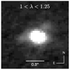 |
Fig. A.1. Image from the R100 data cube combined with a pixel scale of 0.03″ in the wavelength range 1μm < λ < 1.25μm. North is up and east is to the left. In addition to the bright central source, faint emission was detected in the east and north-west and is either associated with the AGN host galaxy GS_3073 or low-mass companions. |
Appendix B: Line fluxes of He I
In Table B.1, we report the total (narrow+outflow+BLR) line fluxes of the seven He I lines detected in the integrated spectrum of GS_3073 (see Figure 1) normalised to the total line flux of He Iλ4471. We verified that choosing a larger aperture would not significantly modify the line ratios. We note that He Iλ4713 is uncertain due to blending with [Ar IV]λ4711. We found that He Iλ7065 is particularly strong compared to theoretical predictions (e.g. Smits 1996; Benjamin et al. 1999; Del Zanna & Storey 2022), which has also been seen in some other data sets (see e.g. Benjamin et al. 1999). Knowledge of relative He I intensities may be useful in reproducing more complex spectra of type 1 AGN showing prominent Fe II emission in addition to He I (see e.g. Véron-Cetty et al. 2004; Perna et al. 2021).
Total (narrow+outflow+BLR) emission line fluxes of the He I lines detected in the integrated spectrum of GS_3073 as constrained through our best fit (Section 3.2), normalised to He Iλ4471.
Appendix C: Integrated PRISM spectrum
In Figure C.1, we show the PRISM spectrum integrated over the central 24 spaxels and flux-matched to the integrated G395H spectrum discussed in the main text, with flux in log scale. In addition to the emission lines detected in the G395H spectrum and discussed in the main text, we indicate the positions of another 14 emission lines (or emission line doublets). These additional lines cover the range from Lyα to Hγ.
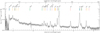 |
Fig. C.1. Integrated spectrum of the PRISM data extracted from a circular aperture containing the central 24 spaxels and flux-matched to the integrated G395H spectrum discussed in the main text, with flux in log scale. We indicate the positions of another 14 emission lines (or emission line doublets) in addition to what is discussed in the main text based on the G395H spectrum. |
All Tables
Total (narrow+outflow+BLR) emission line fluxes of the He I lines detected in the integrated spectrum of GS_3073 as constrained through our best fit (Section 3.2), normalised to He Iλ4471.
All Figures
|
Fig. 1. Integrated spectrum extracted from the central three by three spaxels in the wavelength range 2.86 μm < λ < 4.85 μm with flux in linear scale (top) and log scale (bottom). Several emission lines are present and indicated by vertical lines at the top of the panels. We detected seven He I lines, He IIλ4686, Hβ, [O III]λλ4959, 5007, Hα, [N II]λλ6548, 6583, and [S II]λλ6716, 6731. We also report the detection of [Ar IV]λ4711, [Ar IV]λ4740, and [Ar III]λ7136. (We note that [Ar IV]λ4711 is blended with He Iλ4713.) The auroral line [O III]λ4363 is only partly covered by the spectral band of our observation with the G395H grating. The line [O I]λ6003 falls into the detector gap masked here in the region 4.06 μm < λ < 4.14 μm. The BLR components are present in Hβ, Hα, He II, and in the He I lines. In addition, an outflow component is present and is best visible in the broadened asymmetric line base of the [O III] doublet. In the bottom panel, we indicate with grey dotted vertical lines the positions of possible coronal lines, [Fe XVI], [Ca V], [Fe XIII], [Fe V]; of an auroral line, [N II]λ5755; and of another line at λ ∼ 7167.5 Å, the position of which is consistent with Si I. |
| In the text | |
|
Fig. 2. Zoom-in of the integrated spectrum extracted from the central three by three spaxels including our best fit (blue) with individual components for the emission lines (narrow: green, outflow: orange, BLR: purple) for different wavelength ranges. Left panel: Wavelength range including He IIλ4686, [Ar IV]λ4711, He Iλ4713, [Ar IV]λ4740, Hβ, He Iλ4922, [O III]λ4959, and [O III]λ5007. Right panel: Wavelength range including [N II]λ6548, Hα, [N II]λ6584, He Iλ6678, [S II]λ6716, and [S II]λ6731. The bottom sections of each panel show the residuals, res. = data – best fit. We note that for some of the weaker lines, no BLR or outflow component was preferred by the fit. We further note a faint flux excess red-wards of [O III]λ5007 that is undetected in individual spaxels, potentially suggesting some higher velocity (nuclear) outflow components not captured by our fiducial fit. |
| In the text | |
|
Fig. 3. Projected maps of line flux, velocity, and velocity dispersion. Top and middle row: flux (left), velocity (middle), and velocity dispersion corrected for instrumental resolution (right) as measured from the narrow [O III] component (top) and the narrow Hα component (middle) tracing the host galaxy kinematics. Bottom: flux (left), V10, the velocity at the 10th percentile of the emission-line profile (middle), and V90, the velocity at the 90th percentile (right), from the outflow [O III] component. North is up and East is to the left. The spaxel size is 0.1″. A bar in the first column indicates 1″, corresponding to roughly 6 kpc at the source redshift. The highest projected velocities are found in the East-South-East region in both the narrow Hα and [O III] velocity maps, and are possibly related to an ongoing interaction with a faint companion (see Appendix A). Apart from this region, a velocity gradient of Δv ∼ 70 km s−1 along the North-North-West to South-South-East direction is visible in both the narrow [O III] and Hα, possibly indicative of rotation. There is a small offset between the integrated [O III] and Hα line centroids of about 8 km s−1. We find elevated velocity dispersions in the galaxy centre, as expected for observations of a rotating disc affected by beam smearing. The outflow is visible in the nuclear region, with positive and negative velocities respectively the systemic velocity of |600–700| km s−1. |
| In the text | |
|
Fig. 4. Central black hole mass MBH as a function of host galaxy stellar mass Mstar (left) and host galaxy dynamical mass Mdyn (right) for GS_3073 (blue filled star) and literature compilations. Left panel: Comparison of our galaxy to local AGN by Reines & Volonteri (2015). In this case, the black hole mass was determined from a BLR or from reverberation mapping (red circles, with representative error bar in grey). The black line with a shaded region shows the best fit with uncertainties to this data by Reines & Volonteri (2015), and the dashed lines indicate the intrinsic scatter plus measurement uncertainties. As teal diamonds, we show data by Kocevski et al. (2023) for which we calculated the black hole mass based on Eq. (1) for consistency with our measurement and the z = 0 data. Right panel: Comparison of our galaxy to z ≥ 6 QSOs by Izumi et al. (2021, green diamonds). For our dynamical mass estimate, we adopted a Sérsic index of nS = 4 and an effective radius of Re = 0.18 kpc. We indicated uncertainties by varying Re between 0.11 and 0.9 kpc. The black line shows the local MBH − Mbulge relation with uncertainties and intrinsic scatter by Kormendy & Ho (2013). The black hole of GS_3073 is at the lower end of the MBH − Mdyn distribution when compared to the measurements by Izumi et al. (2021), but it still appears overly massive for its host galaxy’s dynamical mass when compared to the local relation by Kormendy & Ho (2013). Considering the MBH − Mstar relation, the black hole of GS_3073 is much more massive in comparison to local broad line AGN with a similar host galaxy stellar mass. |
| In the text | |
|
Fig. 5. GS_3073 in the mass-metallicity plane (blue star). The z ∼ 0.08 relation based on SDSS data by Curti et al. (2020a) is shown as grey shading with the best fit in black. The red and yellow dash-dotted lines show the best fit relations at z ∼ 2.3 and z ∼ 3.3, respectively, by Sanders et al. (2021) based on data from the MOSDEF survey (Kriek et al. 2015). The dashed green line shows the best fit relation obtained by Nakajima et al. (2023) based on a compilation of early JWST data at redshifts 4 < z < 10. At z = 5.55, GS_3073 is slightly more massive but still compatible with the extrapolation of this relation. |
| In the text | |
|
Fig. 6. Diagnostic diagrams of [O III]λ5007/Hβ versus [N II]λ6584/Hα (left) and [O III]λ5007/Hβ versus [S II]λλ6717,6731/Hα (right). The position of GS_3073 is indicated with the green, purple, and blue filled stars as constrained by its narrow, outflow, and narrow+outflow line ratios, respectively. Local galaxies from SDSS (Abazajian et al. 2009) are indicated by the grey shading, with the contours encompassing 98, 80, and 50 percent of the sample. The red contours encompass 95, 80, and 50 percent of SDSS broad line AGN as classified by Hviding et al. (2022). The dashed line indicates the demarcation by Kauffmann et al. (2003) between galaxies primarily ionised by SF (left) and AGN (right). The dotted lines by Kewley et al. (2001) include more extreme starbursts or composite objects among the star-forming galaxies to the left. The thin coloured symbols (stars, crosses, triangles) show model grids for AGN and direct collapse black holes by Nakajima & Maiolino (2022) for an accretion disc temperature of Tbb = 2 × 10⁵ K, power law indices constraining the slope between the optical and X-ray bands (α = −1.2, −1.6, −2.0, corresponding to stars, crosses, triangles), ionisation parameters (−3.0 < log U < −0.5, indicated by increasing symbol size), and gas phase metallicities (Zgas = 0.001 − 0.028, teal to red colours). A gas density of 103 cm−3 was assumed. Grey symbols show models with lower Tbb. The open circles show model grids for galaxies using BPASS SEDs (Eldridge et al. 2017; Stanway & Eldridge 2018), with binary evolution based on a Kroupa (2001) initial mass function with an upper mass cut of 300 M⊙ and a stellar age of 10 Myr (see Nakajima & Maiolino 2022 for details). Here, the dark to light colours indicate stellar metallicities in the range Z⋆ = 0.0006 − 0.0084. Compared to these theoretical models, GS_3073 has line ratios compatible with being either a low-metallicity AGN or a low-metallicity SFG, despite being located within the classical SFG regime in the diagrams. |
| In the text | |
|
Fig. 7. Diagnostic diagrams of EW(He IIλ4686) versus He IIλ4686/Hβ(left) and He IIλ4686/Hβ versus [N II]λ6584/Hα (right). The symbols are the same as in Fig. 6: Thin stars, crosses, and triangles show evolved AGN and direct collapse black holes; circles show evolved SFGs; and the position of GS_3073 is indicated by the large, filled stars (green: narrow, blue: narrow+outflow, purple: outflow). In the left panel, lines of constant Tbb = 5 × 10⁴ K, 1 × 10⁵ K, 2 × 10⁵ K correspond to dashed, dash-triple-dotted, and dash-dotted lines. In the left panel, the dotted region in the top right indicates the regime expected for Pop III stars. In the right panel, narrow line ratios from local He II-selected AGN by Tozzi et al. (2023) are indicated by the grey shading with contours encompassing 94, 80, and 50 percent of the sample. The dotted line indicates the demarcation by Shirazi & Brinchmann (2012) separating SFGs (left) from AGN (right) at z = 0. In the EW(He IIλ4686) versus He IIλ4686/Hβ diagram, GS_3073 is compatible with an AGN with a hot accretion disc and is clearly separated from SFGs. This is also the case for the He IIλ4686/Hβ versus [N II]λ6584/Hα diagnostic (right), although the locally constrained demarcation line by Shirazi & Brinchmann (2012) appears to evolve with redshift if we consider the location of the model predictions, particularly for AGNs with α = −2.0 (thin triangles). |
| In the text | |
|
Fig. 8. Mass outflow rate Ṁout,ion (left) and kinetic power Pk,ion (right) of the warm ionised gas phase as a function of AGN bolometric luminosity Lbol. The grey circles show ionised gas outflows at 0 < z < 3.5 by Fiore et al. (2017), the green stars show two z ∼ 6.8 QSOs from the GA-IFS GTO programme by Marshall et al. (2023), and the blue stars show the range of bolometric luminosities inferred for GS_3073, as discussed in Sect. 4.1. We have scaled the measurements by Fiore et al. (2017) and Marshall et al. (2023) to correspond to an electron density in the outflow of ne = 1000 cm−3, as assumed in this work. For Lbol, we indicate a representative error bar of 0.5 dex, and for Ṁout,ion and Pk,ion, we indicate how much they would change if ne, Rout, or vout were different by factors 1/5, 5, and 2/3, respectively (see main text for details). The dashed line in the left panel is a linear fit in logarithmic scales to the data by Fiore et al. (2017). The dashed lines in the right panel show constant ratios of Pk and Lbol. The outflow energetics of GS_3073 in relation to the bolometric AGN luminosity are consistent with lower−z scaling relations, suggesting that the driving mechanisms in z > 5 AGN do not differ from their lower−z counterparts. |
| In the text | |
|
Fig. A.1. Image from the R100 data cube combined with a pixel scale of 0.03″ in the wavelength range 1μm < λ < 1.25μm. North is up and east is to the left. In addition to the bright central source, faint emission was detected in the east and north-west and is either associated with the AGN host galaxy GS_3073 or low-mass companions. |
| In the text | |
|
Fig. C.1. Integrated spectrum of the PRISM data extracted from a circular aperture containing the central 24 spaxels and flux-matched to the integrated G395H spectrum discussed in the main text, with flux in log scale. We indicate the positions of another 14 emission lines (or emission line doublets) in addition to what is discussed in the main text based on the G395H spectrum. |
| In the text | |
Current usage metrics show cumulative count of Article Views (full-text article views including HTML views, PDF and ePub downloads, according to the available data) and Abstracts Views on Vision4Press platform.
Data correspond to usage on the plateform after 2015. The current usage metrics is available 48-96 hours after online publication and is updated daily on week days.
Initial download of the metrics may take a while.