| Issue |
A&A
Volume 676, August 2023
|
|
|---|---|---|
| Article Number | A27 | |
| Number of page(s) | 17 | |
| Section | Interstellar and circumstellar matter | |
| DOI | https://doi.org/10.1051/0004-6361/202039923 | |
| Published online | 01 August 2023 | |
Dense gas and star formation in the outer Milky Way
1
Laboratoire d’Astrophysique de Bordeaux, Univ. Bordeaux, CNRS,
B18N allée Geoffroy Saint-Hilaire,
33615
Pessac, France
e-mail: This email address is being protected from spambots. You need JavaScript enabled to view it.
2
Purple Mountain Observatory, Chinese Academy of Sciences,
10 Yuanhua Road,
Nanjing
210023, PR China
3
Kyushu Kyoritsu University,
Jiyugaoka 1-8, Yahatanishi-ku, Kitakyushu,
Fukuoka
807-8585, Japan
4
SRON Netherlands Institute for Space Research,
Landleven 12,
9747 AD
Groningen, The Netherlands
5
Kapteyn Astronomical Institute, University of Groningen,
The Netherlands
6
Laboratoire d’Astrophysique (AIM), CEA/DRF, CNRS, Université Paris-Saclay, Université Paris Diderot,
Sorbonne Paris-Cité,
91191
Gif-sur-Yvette, France
7
Research Center for Intelligent Computing Platforms, Zhejiang Laboratory,
Hangzhou
311100, PR China
8
Department of Astronomy, Xiamen University,
Xiamen, Fujian
361005, PR China
Received:
16
November
2020
Accepted:
1
June
2023
Abstract
We present maps and spectra of the HCN(1−0) and HCO+(1−0) lines in the extreme outer Galaxy, at galactocentric radii between 14 and 22 kpc, with the 13.7 m Delingha telescope. The nine molecular clouds were selected from a CO/13CO survey of the outer quadrants. The goal is to better understand the structure of molecular clouds in these poorly studied subsolar metallicity regions and the relation with star formation. The lines are all narrow, less than 2 km s−1 at half power, enabling the detection of the HCN hyperfine structure in the stronger sources and allowing us to observationally test hyperfine collision rates. The hyperfine line ratios show that the HCN emission is optically thin with column densities estimated at N(HCN) ≈ 3 × 1012 cm−2. The HCO+ emission is approximately twice as strong as the HCN (taken as the sum of all components), in contrast with the inner Galaxy and nearby galaxies where they are similarly strong. For an abundance ratio χHCN/χHCO+ = 3, this requires a relatively low-density solution for the dense gas, with n(H2) ~ 103−104 cm−3. The 12CO/13CO line ratios are similar to solar neighborhood values, which are roughly 7.5, despite the low 13CO abundance expected at such large radii. The HCO+/CO and HCO+/13CO integrated intensity ratios are also standard at about 1/35 and one-fifth, respectively. The HCN is weak compared to the CO emission, with HCN/CO ~ 1 /70 even after summing all hyperfine components. In low-metallicity galaxies, the HCN deficit is attributed to a low [N/O] abundance ratio; however, in the outer disk clouds, it may also be due to a low-volume density. At the parsec scales observed here, the correlation between star formation, as traced by 24 μm emission as is standard in extragalactic work, and dense gas via the HCN or HCO+ emission is poor, perhaps due to the lack of dynamic range. We find that the lowest dense gas fractions are in the sources at high galactic latitude (b > 2°, h ≳ 300 pc above the plane), possibly due to lower pressure.
Key words: galaxies: ISM / galaxies: individual: Milky Way / ISM: clouds / ISM: molecules / stars: formation / local insterstellar matter
Deceased.
© The Authors 2023
 Open Access article, published by EDP Sciences, under the terms of the Creative Commons Attribution License (https://creativecommons.org/licenses/by/4.0), which permits unrestricted use, distribution, and reproduction in any medium, provided the original work is properly cited.
This article is published in open access under the Subscribe to Open model. This email address is being protected from spambots. You need JavaScript enabled to view it. to support open access publication.
1 Introduction
A general theory of star formation needs to be tested in multiple environments. Most work (see e.g., Kennicutt & Evans 2012) has studied galactic disk star formation (SF), SF in bright and perturbed environments such as mergers or ultraluminous galaxies (ULIRGs), or bright low-metallicity objects such as blue dwarf galaxies. Observations of the outer Galaxy provide a new environment for the study of the SF cycle (H I to H2 to stars). The outer disk is cooler and has a lower gas content and, in particular, less molecular gas than the brighter regions mentioned above. The star formation rate (SFR) is low (see e.g., Sodroski et al. 1997) and the metallicity is subsolar but not extremely low in the outer disk (gradient of ≈0.04 dex kpc−1, Pedicelli et al. 2009). The morphology and gravitational potential are those of a rotating disk, unlike mergers and many dwarfs. Finally, the outer disk, defined as beyond the R25 radius, is typically where the gas surface density exceeds that of stars (see e.g., Fig. 7 of Kennicutt & Evans 2012 or Fig. 1 of Hoekstra et al. 2001). For a population of sun-like stars, a brightness of 25 mag per square arcsecond, defining the R25 radius, corresponds to a stellar surface density of 6.6 M⊙pc−2. Hence, the outer Galaxy represents a new environment (where Σgas ≳ Σ*) for the study of the SF cycle.
A further motivation comes from the observations and simulations showing that galaxies continue to be fueled by inflowing gas (see Linsky 2003; Schmidt et al. 2016, and references therein), particularly when a bar (i.e., a nonaxisymmetric potential) is present, as is the case for the Galaxy. Thus the outer disk represents a part of the future of our Galaxy.
The SFR at kiloparsec scales is well known to be linked to the presence of gas and particularly molecular gas (e.g., Kennicutt 1989). Closer to cloud scales, the cloud life cycle (pre-SF, embedded SF, exposed SF, and cloud dispersal) is such that much more scatter is present in the SFR-H2 relation. More recently, the link between the dense gas mass, generally as traced by the high-dipole moment molecules HCN or HCO+, has been shown to be approximately linear in galactic disks at both kilo-parsec (e.g., Gao & Solomon 2004b,a; Kepley et al. 2014; Chen et al. 2017; Braine et al. 2017) and parsec scales (e.g., Wu et al. 2010; Shimajiri et al. 2017) with approximately the same SFR/Mgas ratio (see Fig. 13 of Jiménez-Donaire et al. 2019). In galactic centers, the SFR/Mgas ratio is clearly lower than in disks (see lower panel of Fig. 7 in Chen et al. 2015; Usero et al. 2015). Table 5 and Fig. 13 of Jiménez-Donaire et al. (2019) show that over about ten orders of magnitude in LHCN, there is a scatter of 0.37 dex in the LIR/LHCN ratio, where LIR traces the SFR, in agreement with Gallagher et al. (2018).
Far-IR observations with the IRAS satellite and the follow-up in CO by Wouterloot & Brand (1989) revealed molecular gas out to a galactocentric distance of about 18 kpc. Perhaps surprisingly, Digel et al. (1994) found several molecular clouds beyond 18 kpc; however, they are all much less CO-bright (although of comparable mass) than Orion viewed at a similar distance and resolution. The atomic gas extends considerably further (e.g., Kalberla & Kerp 2009), but with little or no evidence of SF or young stars.
Recent increases in mapping speed and receiver bandwidth combined with post-IRAS far-IR surveys such as Herschel Hi-Gal (Molinari et al. 2016) and APEX Atlasgal (Schuller et al. 2009) has led to revived interest in the outer Galaxy. Sun et al. (2015) surveyed a vast region covering 100 < l < 150° and −3 < b < 5.25° in the J = 1−0 transition of CO and isotopologues to determine how much molecular gas is present at large galactocentric distances. In addition to previously known clouds, they found 49 previously undetected extreme outer Galaxy clouds (Rgal > 14 kpc). The CO emission is generally quite weak, with integrated intensities below 10 K km s−1 at the CO peaks. 13CO(1−0) and C18O(1−0) were observed simultaneously and the images and spectra are presented in Sun (2015). 13CO(1−0) emission is detected in nearly half of the sources. The 12CO/13CO line ratio is typically about five in peak temperature and seven in integrated intensity; the C18O lines were not detected (see Sect. 4.1).
Sun (2015) started a comparison between SF and the presence of molecular gas in the outer Galaxy. One of the results of her thesis was that while SF was not always associated with molecular gas in these extreme outer Galaxy clouds, the clouds hosting young stellar objects (YSOs) were generally more massive than those without YSOs. Here we pursue the comparison between tracers of SF and molecular gas in the outer Galaxy, focusing on the link between dense gas and SF. At kiloparsec scales, there is a good correlation between the dense gas mass and the SFR (Chen et al. 2015) as for whole galaxies (Gao & Solomon 2004b). The low-J transitions of the high-dipole moment molecules HCN and HCO+ are standard tracers of dense gas because high densities (close to 105 cm−3) are required for collisional excitation (Evans 1999). However, the lines are much (factor 10–100) weaker than the CO lines so the existing 12CO(1−0) and 13CO(1−0) observations were used to define regions to be observed in HCN and HCO+ in the extreme outer Galaxy. The dataset obtained is used to explore the physical conditions of the molecular medium far out in the Galaxy and the link between dense gas and SF in a new environment (e.g., Glover & Clark 2012). There is evidence that HCN is more sensitive to metallicity variations than HCO+ (Rudolph et al. 2006; Nishimura et al. 2016; Braine et al. 2017). The outer Galaxy has a subsolar metallicity, but also a generally weak UV field and thus provides complementary information to observations of low-metallicity galaxies, which often have high UV fields.
Only a few observations of dense gas tracers in the outer Galaxy have been made (Yuan et al. 2016), so we significantly increase this sample. Yuan et al. (2016) observed a large sample of Planck Galactic cold clumps, detected in the submillimeter range by the Planck satellite and generally close to the Sun. The samples are quite different in that the Sun et al. (2015) survey was blind and none of their 72 sources were detected in the C18 O line. Very recently, Fontani et al. (2022) observed molecular lines, including HCN and HCO+, in a sample of actively star-forming IRAS-selected cores and Patra et al. (2022) mapped the HCN and HCO+ (1−0) lines around regions with massive stars, also in the outer Galaxy. These two samples are quite different from ours, as we subsequently see (Sect. 4.2).
The paper is structured as follows: after presenting the observations and the basic results, we estimate the excitation temperatures, optical depths, and column densities of the CO lines and then for the HCN, where the satellite line strengths are used to estimate the optical depth. In this part, we initially follow Yuan et al. (2016). The following section presents radiative transfer calculations of the HCN line ratios and also the HCN/HCO+ line ratio, in order to constrain the volume density and determine whether the CO-emitting gas can also be responsible for the HCN and HCO+ line emission. We then discuss the line ratios with the goal of understanding why they are not typical of Galactic or most extragalactic observations, and we summarize the results for this rather unique dataset.
2 Cloud sample and observations
The sources were selected from the Sun et al. (2015) sample of outer Galaxy CO clouds. All of the clouds are quite far from the Galactic center, ranging from 14 to 22 kpc with the Reid et al. (2014) rotation curve. Although a different rotation curve will yield slightly different results, these are clearly far outer Galaxy objects, close to or beyond twice the solar circle distance. Sources were chosen to have (a) an integrated CO(1−0) intensity ICO > 7 K km s−1 and (b)  and (c) a peak 13CO temperature above 0.7 Kelvin. The 13CO data are from Sun (2015) and the cloud characteristics, 12CO, and 13CO intensities are provided in Table 1. This yielded a sample of nine clouds: 7, 14, 16, 18, 21, 30, 34, 56 and 57, all of which have13 CO sizes between 2 and 5 square arcminutes and peak CO temperatures above 4 Kelvins. The central positions of all clouds were observed and clouds 21, 56, and 57, the brightest in HCN and HCO+, were mapped. Figure 1 presents WISE 22 μm band images, supposed to trace SF, with the positions observed and symbols indicating class I and class II YSOs. Figure 2 shows the same for the three clouds that were mapped in HCN and HCO+ along with contours of CO intensity. The WISE 22 μm band1 was chosen as it was the only tracer of SF available for all sources.
The YSOs within the clouds were identified with the criteria described in Koenig et al. (2012) using the infrared data from the Two Micron All Sky Survey (2MASS: Skrutskie et al. 2006) and the Wide-field Infrared Survey Explorer (WISE: Wright et al. 2010). We restrain our sources to those with photometric errors less than 0.1 mag for 2MASS data and signal-to-noise ratio greater than 5 for WISE data. The criteria in Koenig et al. (2012) are designed to search for young stars at Class I and Class II stages employing two methods. The first is based on photometry in the WISE 3.4, 4.6 and 12 μm bands. The contamination from extragalactic sources (star-forming galaxies and AGNs), shock emission blobs, resolved PAH emission objects can be removed according to their locations in the [3.4]–[4.6] vs. [4.6]–[12] color–color diagram and their WISE photometry. For the sources not detected in the WISE 12 μm band, YSOs are identified from the dereddened Ks–[3.4] vs. [3.4]–[4.6] color-color diagram. In our work, the extinction used to deredden the photometry is estimated from its location in the J – H vs. H – Ks color–color diagram as described in Fang et al. (2013).
The nominal central positions observed correspond to the CO maxima and not necessarily a peak in SF, as can be seen in Figs. 1 and 2. Below we give the assessment of the SF for each observed region (Sun 2015), starting with the single positions and followed by the maps.
Cloud 7: An IRAS point source is present as well as a class II source within the DLH beam.
Cloud 14: No IRAS point source within the beam but a class I source at beam center.
Cloud 16: No IRAS point source but there is a class II source within the DLH beam.
Cloud 18: No IRAS point source but there is a class II source within the DLH beam.
Cloud 30: No IRAS point source but there is a class II source within the DLH beam.
Cloud 34: Class II source within DLH beam and IRAS source nearby (see Fig. 1).
Cloud 21: IRAS point source and class II source at edge of central beam but within map, which also covers a class I source. Map shows no obvious difference in line ratios at positions with SF.
Cloud 56: No IRAS point source within but a class II source near nominal center. SF (22 μm emission) extends to higher b and HCN/HCO+ emission appears to follow.
Cloud 57: IRAS point source at center and two class I sources, one coincident with the IRAS source. A class II source is also present further from the center.
Class I sources are indicated as circles in Figs. 1 and 2. Class II are shown as squares, following Sun (2015).
The observations were carried out in May 2017 with the 13.7m telescope of the Purple Mountain Observatory (PMO) in Delingha, Qinghai, China, hereafter DLH. The beamsize at the HCN and HCO+ J = 1−0 frequencies is 1′ which corresponds to a linear scale of 3 pc at the typical distance of 10 kpc of our clouds (except clouds 56 and 57 which are further such that the beam size is about 4.3 pc). The Superconducting Spectroscopic Array Receiver system, a nine-beam (3X3beam, with separation of 3 arcmin), sideband- separating receiver (Shan et al. 2012) was used as front end. The fast fourier transform spectrometer with a bandwidth of 1 GHz provides 16384 channels and a spectral resolution of 61 kHz (see details in Shan et al. 2012), leading to a velocity resolution of 0.2 km s−1. The telescope is at an altitude of 3200 m and the weather was good during the observations, leading to system temperatures of 140–150 K.
The standard chopper-wheel calibration was adopted to obtain the antenna temperature, (Kutner & Ulich 1981). Spectral intensities are further converted to a scale of main-beam brightness temperature using  , where the main-beam efficiency ηMB is 0.57 at ~90 GHz (see the status report of the 13.7 m telescope2). Considering the small angular size of our targets traced by CO, and the smaller region traced by dense gas, the position-switching mode was used. Two beams with a separation of 6 arcmin were used to observe on-source pointing and emission-free OFF position simultaneously. The pointing accuracy is estimated to be better than 5 arcsec. The mapping step is 30 arcsec.
Cloud sample.
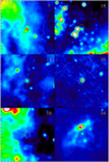 |
Fig. 1 WISE 22 μm band images of sources 7, 14, 16, 18, 30, and 34 (identification in upper right corner). These are the sources for which only a single pointing is available. The images are all 10 arcmin in size, oriented in l and b. The central circle gives the HCN/HCO+ beamsize. The transfer function (rainbow from black to white) of the WISE observations differs from image to image. For cloud 7 it is from 91.5 to 98; for cloud 14 it is 100.5 to 107; for 16 it is 103 to 115; for 18 it is 102 to 114; for 30 it is from 108 to 112 and for cloud 34 it is from 108 to 135 counts. Following Sun (2015), class I sources within our maps are shown as circles and class II as squares. |
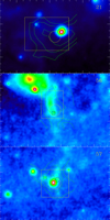 |
Fig. 2 WISE 22 μm band images of sources 21, 56, and 57 (identification in upper right corner). These are the sources which were mapped. The images are all 600″ × 400″ in size, oriented in l and b. The color scale (rainbow from black to white) of the WISE observations differs from image to image. For cloud 21 it is from 95 to 116 and for clouds 56 and 57 the range is from 129 to 134 counts. The central circle gives the HCN/HCO+ beamsize and is the (0,0) position in Figs. 4–6 which show the spectra. The box indicates the size of the region shown in Figs. 4–6. Following Sun (2015), class I sources within our maps are shown as circles and class II as squares. |
3 Results
3.1 Maps and spectra
Table 1 provides source numbers, positions, 12CO intensities, galactocentric distance Rgal, heliocentric distance, all from Sun et al. (2015), and 13CO intensities from Sun (2015). The CO data are on the main beam scale (i.e., corrected for telescope efficiency) and come from observations with the Delingha telescope which has a beam size of 48″ at the CO(1−0) frequency.
In Galactic observations, several clouds can be found along the line of sight at different velocities. More common in the inner Galaxy, this is also the case for these outer Galaxy observations. The outer Galaxy CO survey (Sun et al. 2015; Sun 2015) covered not only the peaks but a vast region in the outer Galaxy and thus maps of each cloud. The spectra and maps of the clouds in the appendix of Sun (2015) show that generally the CO and 13CO is strongest in the distant cloud we are interested in and that even when this is not the case (only cloud 30), the clouds can be visually separated in the maps.
The new observations of the HCN(1−0) and HCO+(1−0) lines are shown along with the pre-existing 12CO(1−0) and 13CO(1−0) lines in Figs. 3–6. The temperature scales are the same from one figure to another so that the figures can be straightforwardly compared. We immediately see that the HCN(1−0) and HCO+(1−0) lines were detected in all sources and that the HCO+ line is systematically stronger than the HCN line. Central velocities are very similar (generally ± one channel) and the optically thick 12CO line is generally broader (by ~40%) than the dense gas tracers (compare Table 2 with Table 1 of Sun et al. 2015).
Table 2 presents the results of the HCN and HCO+ observations. The integrated intensity, velocity, and line width are given for the central spectra in the HCO+(1−0) line and for the main line of HCN(1−0). Clouds 21, 56, and 57 were partially mapped in HCN and HCO+ and the lines indicated by sum are the fits to the coadded (i.e., summed) spectra. The summed spectra have considerably higher signal-to-noise ratios (see last column) so the individual hyperfine components were fit and the results are presented in the same way.
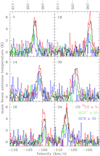 |
Fig. 3 Spectra for the clouds that have not been mapped, as in Fig. 1. The axes are the same for each cloud. 12CO is in black and corresponds to the temperature scale. 13CO is in red and has been multiplied by 5. HCO+, in green, has been multiplied by 35. The HCN spectra have been multiplied by 35 for comparison with HCO+ but also multiplied by 9/5 to account for the satellite lines as explained in the text. The 12CO and 13CO spectra have been convolved with a Gaussian kernel to the angular resolution of the HCN and HCO+ spectra. |
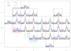 |
Fig. 4 Spectra of Cloud 21. Positions are indicated on the x and y axes as offsets in arcminutes and each box represents 30″. 12CO is in black, 13CO in red, HCO+ in green and HCN in blue. The velocity scale goes from −106.5 km s−1 to −97 km s−1. The temperatures scales are −.7 to 7 K for 12CO, −.14 to −1.4 K for 13CO, −.02 to .2 for HCO+ and for HCN. The HCN line (only central component shown) has been multiplied by 9/5 so that the line intensity represents the total line flux for comparison with other species. The 12CO and 13CO spectra have been convolved to the same angular resolution as the HCN and HCO+. |
3.2 HCN hyperfine structure
HCN and HCO+ are considered to be tracers of dense gas due to their high electric dipole moment. Their critical densities, where collisional de-excitation equals spontaneous de-excitation (see Eq. (4) and Table 1 of Shirley 2015), are ncrit,HCN(1−0) ≈ 4 × 105 cm−3 and  . These densities are roughly 2 orders of magnitude higher than for CO so the typical molecular cloud densities at which CO is collisionally excited do not suffice to generate detectable HCN or HCO+ emission. The outer galaxy environment is cool, with a weak radiation field, and as we shall see the HCN lines are optically thin or nearly so.
Due to the nuclear quadrupole moment of Nitrogen (14N), there is hyperfine structure which is observable in the ground-state rotational transition (J = 1 → 0). Three lines are present and the line ratios can be used to estimate optical depth. The main line is the F = 2 → 1 transition at 88.63185 GHz, with satellite lines F = 1 → 1 and F = 0 → 1 shifted by respectively 4.8 and −7 km s−1. Figure 7 shows the coadded HCN(1−0) spectra for clouds 21, 56, and 57. The individual spectra do not have a sufficiently high signal-to-noise ratio to measure the HFS at individual positions, particularly for the weakest component. The spectra are presented for each cloud separately in Figs. 4–6, which show that the coadded spectra are from regions with strong CO (and 13CO) emission. The second-strongest component is clearly visible in the individual spectra of cloud 56 (Fig. 5) which has the lowest noise level (see Table 2). Generally, when spectra are stacked, the velocity is recentered because the stacking concerns gas at different velocities – this shifting introduces additional uncetainties because of the way the velocity difference is determined. This is not the case here which is why we say “summed” or “coadded” rather than stacked.
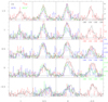 |
Fig. 5 Spectra of Cloud 56. Positions are indicated on the x and y axes as offsets in arcminutes and each box represents 30″. 12CO is in black, 13CO in red, HCO+ in green and HCN in blue. The velocity scale goes from −107.5 km s−1 to −99 km s−1. The temperatures scales are −.7 to 7K for 12CO, −.14 to 1.4K for 13CO, −.02 to .2 for HCO+ and for HCN. The HCN line (only central component shown) has been multiplied by 9/5 so that the line intensity represents the total line flux for comparison with other species. The spectra in the corners show only CO as not all positions were observed in HCN and HCO+. |
3.3 Relative line intensities
As can be seen in Figs. 8 and 9, the CO and 13CO, and HCN and HCO+ line fluxes are correlated. The relation is approximately  for the set of data. The correlation coefficients are r = 0.62 between dense gas tracers and r = 0.65 between the 12CO and 13CO lines. Mixing the dense and total gas tracers, for respectively CO-HCO+, CO-HCN, 13CO-HCO+, and 13CO-HCN, the correlation coefficients are 0.53, 0.44, 0.44, and 0.43. Hence, the total gas mass (clouds) and dense gas mass (cores) are linked but the dense gas tracers (HCN, HCO+) are more strongly correlated with each other, as are the general molecular gas tracers (CO, 13CO), than with clouds and cores.
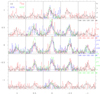 |
Fig. 6 Spectra of Cloud 57. Positions are indicated on the x and y axes as offsets in arcminutes and each box represents 30″. 12CO is in black, 13CO in red, HCO+ in green and HCN in blue. The velocity scale goes from −106.5 km s−1 to −98 km s−1. The temperatures scales are −.7 to 7 K for 12CO, −.14 to 1.4 K for 13CO, −.02 to .2 for HCO+ and for HCN. The HCN line (only central component shown) has been multiplied by 9/5 so that the line intensity represents the total line flux for comparison with other species. The spectra in the corners show only CO as not all positions were observed in HCN and HCO+. |
4 Physical conditions from an LTE analysis
In this section, we apply the standard formulae to estimate optical depths and column densities of the species presented here. The formulae are presented in Yuan et al. (2016), Mangum & Shirley (2015), and Shirley (2015) and the works cited therein. We initially follow the reasoning in Yuan et al. (2016) for straightforward comparison and then present another approach. Without making ad hoc hypotheses, it is difficult to make non-local thermodynamic equilibrium (LTE) calculations so the following section presents radiative transfer calculations with RADEX (van der Tak et al. 2007).
The observations are of clouds between 14 and 22 kpc from the Galactic center so we expect abundances to be subsolar (e.g., Pedicelli et al. 2009) and we follow the Pineda et al. (2013) 12/13C gradient (see Eq. (4) in Yuan et al. 2016) and the Fontani et al. (2012) 12CO abundance gradient (see Eq. (7) in Yuan et al. 2016).
4.1 Molecular column densities: 12CO(1−0) and 13CO(1−0)
Following Yuan et al. (2016) Eqs. (3) and (4), we estimate the 13CO(1−0) optical depth, τ13, and, multiplying by the 12/13C ratio, the optical depth of the main line, τ12. This assumes that excitation temperatures and surface filling factors (fraction of the beam occupied by emitting molecules) are the same for both isotopologues. The 13CO(1−0) emission is optically thin, with 0.15 < τ13 < 0.32 calculated in this way, yielding main isotope optical depths on the order of 20. C18O(1−0) emission was not detected in these sources, confirming the low optical depths of the 13CO(1−0) emission.
Assuming a filling factor of unity, the observed brightness temperature can be used to calculate the excitation temperature of the 12CO(1−0) line. The optical depths obtained previously mean that the main line is highly optically thick so that it does not enter in the excitation temperature calculation (see e.g., Eq. (88) of Mangum & Shirley 2015) but also that the 13CO(1−0) column density is almost independent of τ13; but we need to assume that the excitation temperatures are the same (or known) for both isotopologues as in Yuan et al. (2016). The excitation temperatures vary from 7.3 to 11.4 K for the nine sources, apparently reasonable values for the outer Galaxy. Table 3 shows the optical depths, excitation temperatures, CO column densities, and H2 column density based on the 12CO and 13CO column density (see Sect. 4.5). Table 4 provides the limits to the C18O(1−0) emission, obtained by averaging C18O and 13CO spectra over the maps.
However, as explained in Shirley (2015), the effective critical density is lower than the standard value for highly optically thick lines such as 12CO(1−0) but not the optically thin 13CO(1−0). As a result, we expect that our hypothesis of equal excitation temperatures is inappropriate and we test lower excitation temperatures for 13CO(1−0), halfway between the CMB temperature and the 12CO(1−0) excitation temperature Tex,13 = Tbg + 0.5 (Tex,12 − Tbg), so that the 13CO(1−0) alternative excitation temperatures range from 5 to 7 K. While ad hoc, this preserves the order among the sources and remains sufficiently far from Tbg that the column density is not close to diverging. The results with the modified excitation temperature are also given in Table 3.
One may also wonder whether it is reasonable to assume the same filling factor for the two lines, as we expect there to be a low-density region near the edge of the cloud where 12CO is present (self-shielded) but not 13CO. This is likely the case but the external radiation field in these extreme outer galaxy sources is very low so the difference in filling factors should be small. Filling factors are extremely structure-dependent and hence very difficult to estimate, so we have not attempted to change the equal filling factor assumption for 13CO(1−0).
Results of observations of central positions, deduced from Gaussian fits.
4.2 Molecular column densities: HCN(1−0)
For LTE excitation, which is expected given that the energy levels are so close, the optically thin hyperfine line ratios should be 5:3:1 (i.e., 0.6 and 0.2 when compared to the main line) due to the degeneracies of the levels (2F+1), such that the total HCN line strength is 1.8 times that of the main component. Figure 10 shows the HFS line ratios expected as a function of the optical depth of the main line. Cases of “anomalous” line ratios exist but these all result in a high  ratio (Kwan & Scoville 1975; Guilloteau & Baudry 1981) and generally involve high optical depth and/or double-peaked profiles. The (F = 1 → 1)/(F = 2 → 1) and (F = 0 → 1)/(F = 2 → 1) line ratios for clouds 21, 56, and 57 are respectively 0.57 and 0.21, 0.60 and 0.18, 0.69 and 0.325. These values are indicated on Fig. 10 and indicate that the HCN emission from clouds 21 and 56 is optically thin (τ ≲ 0.5) but cloud 57 has an optical depth τ ~ 1. The agreement is excellent between the two line ratios for all three clouds.
An independent estimate can be obtained by following Yuan et al. (2016) who use the CLASS3 hyperfine structure method to fit the three lines of the summed spectra of clouds 21, 56, and 57. In addition to velocity and velocity width, this method estimates the optical depth of the main line. The optical depths obtained are τ21 = 0.24 ± 0.15, τ56 = 0.66 ± 0.10, τ57 = 1.50 ± 1.47 for clouds 21, 56, and 57, respectively, in good agreement with the previous estimates.
Because these are line ratios of the same molecule at essentially the same energy, the optical depths are those after taking into account any filling factor, such that they are not beam-averaged. The “naive” and CLASS estimates are consistent with optically thin (τ < 1) HCN emission from clouds 21 and 56 and τ ≈ 1 in cloud 57.
Optically thin means we can estimate the column density from the line intensity. If we assume that the HCN excitation temperature is that of CO, then the column densities range from 3 × 1010 cm−2 to 2 × 1011 cm−2 (cloud 57). If we assume that the HCN excitation temperature is between the CMB temperature and that of CO (see previous section for 13CO), then the column densities are a factor 3 higher, ranging from 1011 cm−2 to 7 × 1011 cm−2 (cloud 57). Yuan et al. (2016) assume a very low excitation temperature, where Tex = 2hB/k (the first energy level, 4.25 K for HCN), and this yields much higher HCN column densities. These column densities are beam-averaged because they use the integrated intensities, unlike the optical depths calculated earlier from the HFS ratios. The column densities for the three excitation temperatures are provided in Table 3 but our fiducial value is the intermediate one.
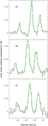 |
Fig. 7 Sum of spectra for each of the clouds for which we were able to make maps. The lines are narrow although each spectrum represents a sum of many positions. The clear separation of the hyperfine components enables us to estimate the optical depth. The parameters of the Gaussian fits shown in green are given in Table 2. |
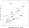 |
Fig. 8 Integrated intensities of HCN and HCO+ lines for all positions observed. All data are on the main beam temperature scale and the central HCN intensity has been multiplied by 9/5 to account for the satellite hyperfine components. The line indicates |

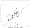 |
Fig. 9 Integrated intensities of 12CO and 13CO lines for all positions observed. The line indicates the best-fit: |

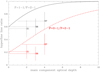 |
Fig. 10 LTE representation of hyperfine component ratios as a function of main component (F = 2−1) optical depth. The observed ratios for clouds 21, 56, and 57 are indicated. The vertical dashed lines indicate the uncertainties from Table 3. |
13CO(1−0) and C18O(1−0) intensities averaged over the maps.
4.3 Molecular column densities: dense gas filling factor
Because we have an estimate of the optical depth, we can estimate the filling factor by rearranging Eq. (2) of Yuan et al. (2016) as follows:
![Mathematical equation: ${T_{\rm{r}}} = {{hv} \over k}\left[ {J\left( {{T_{{\rm{ex}}}}} \right) - J\left( {{T_{{\rm{bg}}}}} \right)} \right]\,\tau \,f,$](/articles/aa/full_html/2023/08/aa39923-20/aa39923-20-eq17.png) (1)
(1)
where J(T) = [exp(hv/kT) − 1]−1 which becomes
![Mathematical equation: $f = {{k\,{T_{\rm{r}}}} \over {hv\tau }}{\left[ {J\left( {{T_{{\rm{ex}}}}} \right) - J\left( {{T_{{\rm{bg}}}}} \right)} \right]^{ - 1}}.$](/articles/aa/full_html/2023/08/aa39923-20/aa39923-20-eq18.png) (2)
(2)
We use the optically thin approximation (1 − exp(−τ)) ≈ τ but at the moderate optical depths present here this has little effect. We can then use the values of τ to deduce a limit for the filling factor f for the two Tex above.
In order to apply this reasoning to the other sources, we can average the 3 optical depths obtained from the CLASS fits. We obtain < τ > ≈ 0.53 when weighting either by the inverse of the uncertainty or by the square of the inverse of the uncertainty. We apply this to the weaker sources which were not mapped, hence probably over-estimating τ. The filling factors obtained range from 4 to 16% for our fiducial HCN(1−0) excitation temperature, see Table 3. Wang et al. (2020) found dense gas filling factors of 6–28% in the molecular filament GMF54 (Ragan et al. 2014) over the regions where 13CO was detected (equally our case), so the values we find appear reasonable. GMF54 is beyond the molecular ring and few appropriate comparison sources are available. We then expect the true (not beam-averaged) column densities to be a factor 1/f times higher (Col. 10 divided by Col. 14 in Table 3). This yields HCN column densities for the cores of ≈2 × 1012 cm−2 except for clouds 56 and 57 which may reach 1013 cm−2. Note that this is for the total line width and not per km s−1 and assumes that the dense gas occupies a relatively small fraction of the beam.
4.4 Molecular column densities: HCO+(1−0)
HCO+ is believed to be less abundant than HCN (Godard et al. 2010; Watanabe et al. 2017) and the turbulent linewidths and dipole moments are similar such that if HCN is optically thin, then HCO+ should be as well. Taking HCO+ to be optically thin, we can do the same calculations, again assuming our fiducial excitation temperature midway between Tbg and Tex,CO (Sect 4.1). The column densities are given in Table 3. We can see that overall the HCN and HCO+ column densities are similar:  (see Cols. 10 and 13 of Table 3).
Having established that the HCN(1−0) line, and likely the HCO+ line, are optically thin or nearly so, we can ask ourselves whether the apparently similar HCN and HCO+ column densities necessarily reflect the true abundance ratio. The critical density of HCN is about 7 times higher than that of HCO+ (see Shirley 2015, Table 1 or, for HCO+, Fig. 3 extrapolating to our column densities), potentially resulting in more severely subthermal excitation for the HCN line. This could reduce the HCN line intensities, from which we estimate the column densities, more than the HCO+, such that the true HCN/HCO+ abundance ratio could be higher. As it is difficult analytically, the following section will explore this more quantitatively via non-LTE calculations.
4.5 Molecular column densities: H2
Observations of 12CO(1−0), 13CO(1−0), HCN(1−0), and HCO+(1−0) have been presented. The latter two molecules are considered dense gas tracers as their critical densities are about 100 times higher than for CO where ncrit ≈ 1000 cm−3and less when highly optically thick. We can estimate the average H2 column density from the CO observations by simply dividing by the fractional abundance (Pineda et al. 2013; Fontani et al. 2012), such that  or
or  where the column densities are given in Cols. 5 and 8 of Table 3. The N(H2) values are presented in the last two columns of Table 3. The H2 column densities derived in this way are significantly higher than when using the standard large-scale N(H2)/ICO factor used in extragalactic observations (e.g., Bolatto et al. 2013). This is expected as the CO emission from the outer galaxy is weak compared to the inner galaxy (Sodroski et al. 1995; Digel et al. 1994), presumably due to lower abundances and lower temperatures. Extragalactic observations by Sandstrom et al. (2013) found that the N(H2)/ICO ratio did not change significantly within the inner disk (out to 0.7 R25). However, the positions observed here are far beyond R254 and the ratios we find by dividing the N(H2) from Table 3 by ICO from Table 1 are still within the scatter of their Fig. 4, and therefore there is no conflict.
Rather standard values of N(H2) are found, on the order of 1022H2 cm−2, suggesting that the procedure is reasonable and that outer galaxy, even extreme outer galaxy, molecular clouds have similar masses and column densities as local clouds. Taking the maps in Figs. 4–6 as representative of the size of the clouds, we obtain sizes of 10–15 pc. If the depth is the same, the average density (i.e., for a volume filling factor of unity) is < n > ≈ 1022/3 1019 ≈ 300 cm−3. This is sufficient to thermalize the highly optically thick 12CO(1−0) line but not the HCN or HCO+. In order to reach densities where the dense gas tracers are excited, either the cloud would be a thin sheet with a line-of-sight depth about 1% of the extent perpendicular to the line of sight, or the HCN and HCO+ emission is produced by dense clumps within the cloud which do not contribute significantly (> 10%) to the cloud mass or the 12CO(1−0) emission. We subsequently assume the latter.
It is difficult to estimate the H2 column density of the dense clumps as the HCN and HCO+ abundances are not well known. HCN sticks to dust and is thus less abundant in cool dense environments. Lahuis & van Dishoeck (2000) suggest that the HCN abundance with respect to H2 is χHCN ≈ 10−8 and higher in hot environments. In the outer Galaxy clouds, we are clearly not in the “hot environment” case. A study of Planck cold cores by Yuan et al. (2016) found very low abundances, roughly 1.5 × 10⁻¹⁰ for both HCN and HCO+. Although these clouds were generally much closer, with an average distance of 1.3kpc, this work has the physical conditions closest to the outer disk observations presented here. The Fontani et al. (2022) and Patra et al. (2022) sources (massive star-forming regions) are very different (although in the outer disk) with broader lines, outflows, strong HCN and HCO+ emission and even H13CN emission; they do not estimate abundances. Pirogov et al. (1995) find an HCN abundance χHCN > 10−10 toward a high-latitude cloud. Turner et al. (1997) estimate χHCN > 10−9 from observations of translucent molecular clouds. Watanabe et al. (2012, Watanabe et al. 2017) find χHCN ≈ 10−9 toward a low-mass class 0 protostar and χHCN ≈ 2 × 10⁻⁹ toward W 51, respectively. In their extragalactic work, Gao & Solomon (2004a) assume χHCN = 2 × 10⁻⁸. Watanabe et al. (2014) observed two positions in M 51 and find fractional abundances χHCN ≈ 10−9. Martín et al. (2006) and Aladro et al. (2011) find values within a factor two of 10−9 for respectively NGC 253 and M 82 such that the column density of dense gas is:
 (3)
(3)
where NHCN is the beam-averaged value but, because we divide by the filling factor f,  is the estimated N(H2) of the dense clumps. Note that this expression keeps the HCN abundance as a free parameter but introduces reasonable values in order to provide an illustrative value of the H2 column density. The range of χHCN that we regard as likely in the extreme outer disk environment is 10−9 >χHCN > 10−10.
A beam-averaged HCN or HCO+ column density of a few 1011 cm−2 (Table 3, Cols. 10 and 13) corresponds to beam-averaged dense gas column of  , to be compared with N(H2) ≈ 1022 cm−2 from Cols. 15 and 16 of Table 3. Thus, depending on the abundance, the mass in the clumps dense enough to excite the HCN and HCO+ molecules represents on the order of 10% of the mass.
5 Physical conditions via radiative transfer calculations
The analytical calculations in the previous section are necessarily based on the hypothesis that the molecules are in LTE. LTE is a strong assumption which is probably not valid, particularly for high-dipole moment molecules such as HCN and HCO+. We made a first attempt to account for this by allowing for a lower excitation temperature for the optically thin (or nearly so) molecular emission. In this section we make non-LTE calculations in order to go a step further and in particular to treat the HCN and HCO+ molecules separately because although they both have high-dipole moments, their critical densities are different and the non-LTE transfer calculations enable us to interpret the factor ~2 difference in intensity.
5.1 Model setup
To constrain the volume and column densities of our observed outer Galaxy clouds, we have run a grid of non-LTE models of the HCN and HCO+ line emission using the radiative transfer program RADEX5 (van der Tak et al. 2007). This program solves for the relative populations of the rotational energy levels of the molecules, taking collisional and radiative (de-)excitation into account, and treats the line radiative transfer with an escape probability formalism. The free parameters in the calculation are the kinetic temperature, the gas density, and the molecular column density. In the calculations, we assume a background temperature of 2.73 K, a turbulent line width of 1.0 km s−1, and a uniform medium without velocity gradients. The linewidths of these clouds are slightly above 1.0 km s−1 and any column density per turbulent linewidth should be multiplied by the linewidth (Table 2) to obtain the total column density.
Watanabe et al. (2017) indicate that  on average in the sources they consider (their Figs. 10, 11), with
  . Although somewhat uncertain, we take this abundance ratio for our calculations. The decreasing [N/O] ratio would favor HCO+ in the outer disk but HCO+ requires a source of ionization. The competition between these effects is difficult to evaluate and, to our knowledge, model calculations have not provided insight to this. Based on the estimates in Yuan et al. (2016), we see no evidence for lower HCO+/HCN abundance ratios.
Spectroscopic data for the HCN and HCO+ rotational and hyperfine structure were taken from the Cologne Database for Molecular Spectroscopy (CDMS)6 (Müller et al. 2005). The HCO+ calculations use collision data with H2 by Flower (1999), which cover rotational levels up to J = 20 and temperatures of 40–200 K. For the collisional (de)excitation of the lowest rotation-hyperfine levels of HCN with H2, two calculations exist, which both cover our relevant energy levels (up to J = 8–10) and temperatures (down to 5 K and up to 30–100 K), but which differ in the ratio between the rates for radiative (ΔJ = 1) and non-radiative (ΔJ = 0, ΔF = 0,±1) transitions. The calculation by Ben Abdallah et al. (2012) used a potential energy surface for the interaction with a reduced dimensionality, averaging over H2 orientations, and found that collisional deexcitation through non-radiative (cross-F) channels is ≈10× faster than through ΔJ = 1 channels. However, after upgrading the close coupling calculations to full dimensionality, Hernández Vera et al. (2017) found that the collisional deexcitation through both types of channels proceeds at approximately equal rates. For comparison, the quasi-classical calculation by Green & Thaddeus (1974) did not resolve the hyperfine structure of HCN and used He as collision partner. The corresponding datafile on the Leiden Atomic and Molecular Database (LAMDA; Schöier et al. 2005)7 assumes that the radiative transitions have equal collision rates, while the cross-F rates are zero. For lack of experimental data on the relative propensities of cross-F rates, we have explored all 3 sets of collision rates in our models for HCN.
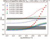 |
Fig. 11 Intensity ratios of the hyperfine components of the HCN J = 1−0 line, calculated with RADEX as a function of N(HCN). Gray areas indicate observed ranges for the F = 1−1/2−1 (top) and 0−1/2−1 (bottom) ratios, respectively 0.6, 0.6, 0.7 and 0.2, 0.2, 0.3 for clouds 21, 56, and 57. The numbers indicating the rates refer to the years of publication of the rates. |
5.2 Model results
To constrain the column densities of the clouds, we model the intensity ratios of the hyperfine components of the HCN J = 1−0 transition. Figure 11 shows the result for an assumed Tkin of 10 K and n(H2) = 104 cm−3, and calculations for Tkin in the 10–30 K range and n(H2) in the 103−3 × 104 cm−3 range indicate that our results depend only weakly on the assumed gas density and kinetic temperature. Column densities of N(HCN) ≈3 × 1012 cm−2 are seen to be consistent with both observed ratios (indicated by the gray areas), but only if the Hernández Vera et al. (2017) collision data with the similar cross-F and cross-J rates are used. Using the data with the large cross-F rates, there is no column density of HCN which matches both observed ratios simultaneously. The collision data with the cross-F rates equal to zero are also able to match the observed hyperfine ratios, but the inferred N(HCN) is less reliable since these hyperfine collision rates were assumed rather than calculated. These rates also lead to unrealistically high hyperfine ratios toward high HCN column densities. The models also reproduce the observed absolute intensities of the HCN lines, for similar column densities as indicated by the hyperfine ratios. We conclude that the HCN line emission indicates N(HCN) ≈ 3 × 1012 cm−2, using the collision data by Hernández Vera et al. (2017).
To constrain the volume densities of the clouds, we model the ratios of the HCN and HCO+ J = 1−0 lines. These calculations assume Tkin = 20 K and an abundance ratio of [HCN]/[HCO+] = 3 (Watanabe et al. 2017). Figure 12 shows the result as calculated with RADEX using the HCN collision rates by Hernández Vera et al. (2017). Our observed line ratio of ≈1/2 (summed over the HCN hyperfine components) is seen to correspond to H2 densities in the 103–104 cm−3 range. The analytical calculations in the previous section yielded similar HCN and HCO+ columns but the degree of subthermal excitation could not be assessed. Nonetheless, if  , then a higher density would be required to yield the observed HCN/HCO+ line ratio. For example, if
  (and not 1/3), then we would deduce a density of n(H2) ≈ 104.5 cm−3.
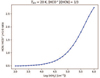 |
Fig. 12 Intensity ratio of the HCN and HCO+ J = 1−0 lines, calculated with RADEX as a function of n(H2). |
5.3 HCN and HCO+ as dense gas tracers
Depending on the HCN and HCO+ abundances, the H2 column density deduced from HCN could be comparable to that deduced from the CO observations (Table 3). Can the gas be the same? We can test this using the intensities of the lines. Assuming that the majority of the CO emission comes from gas with a density n ≲ 3000 cm−3 (see discussion in Sect. 4.5), RADEX calculations show that for n ≲ 3000 cm−3, IHCN/ICO ≲ 0.001 (H2 column assumed is 1021 cm−2 with abundances χCO = 10−5 and χHCN = 10−9). Since IHCN/ICO ≳ 0.01 from Tables 1 and 2, the HCN emission does not come from the gas emitting the majority of the CO emission but rather from clumps or cores within the less dense ambient molecular gas. n principle, the CO could come from gas with n > 3000 cm−3. However, not only would the clouds necessarily be much thinner along the line of sight but also the 13CO emission would be quite unusual, much stronger in the higher-J transitions than in 13CO(1−0). The few pieces of data available for the 13CO(2−1) line, or even CO(2−1), at large scales in the outer parts of galaxies suggest that the higher-J transitions are not stronger (Sakamoto et al. 1997; Braine et al. 1993). Hence, in these outer disk clouds, HCN and HCO+ trace dense gas (n > 103 cm−3).
Figure 8 shows that the HCO+ line is on average twice as strong as the HCN line. To make this figure, the HCN(1−0) main line intensities were multiplied by 9/5 to account for the flux in the weaker satellite lines which have low signal-to-noise ratios and thus can add considerable noise to the sum of the intensities. As seen in Sect. 4, the optical depth is low so this procedure should be appropriate. Since both lines are optically thin, we have used RADEX to estimate the typical density at which the HCO+(1−0) is twice the total HCN(1−0) line intensity. For a column density ratio of 3, this occurs at n ≲ 104 cm−3 (Tkin = 20 K). If in fact the HCO+ abundance is higher (than 1/3 of the HCN abundance), then the density implied by the observed flux ratio is higher. A larger fraction of the HCO+ emission, compared to HCN, comes from the lower density CO-emitting gas and this is why the above calculation sets a lower limit to the typical density of the dense component. This is also seen in Fig. 11 of the observations of W3(OH) by Nishimura et al. (2017) which shows that the HCN(1−0)/HCO+(1−0) ratio decreases toward the more extended and more diffuse material.
We obtain a typical clump or core size of L ≈ N/n where N is the dense gas column density defined in Eq. (3) such that
 (4)
(4)
where  is the average molecular mass. Adopting reference values of NHCN = 3 × 1011 cm−2, n = 104cm−3, χHCN = 10−9, and f = 0.1, we can express the clump or core mass as follows by substituting Eq. (3) into Eq. (4)
 (5)
(5)
with a hydrogen fraction of mh = 0.73. The mass in such a clump is on the order of a solar mass but highly dependent on the abundance, such that if χHCN = 10−10 then the clump mass becomes 620 M⊙. The other parameters are constrained by observations: NHCN by the HCN flux, NHCN/f by the HCN optical depth limit, and n by the HCN/HCO+ flux ratio.
6 Link between star formation and dense gas fraction
Gao & Solomon (2004b) suggested that the SFR is proportional to the mass of dense gas such that starburst galaxies have high dense gas masses. In ultraluminous IR Galaxies (ULIRGs), there is generally a huge amount of gas concentrated near the center and hence the dense gas mass (HCN flux) and fraction (typically the HCN/CO flux ratio) are high. Here we examine smaller scales so, to compare dense gas with SF, we have compared these line ratios for positions with and without a class I or II source. The HCN/CO and HCO+/CO flux ratios are marginally higher for the positions with a class I or class II source but not significantly.
Aside from the good correlation between 8 μm and 24 μm emission, the main result is that the HCN/CO and HCO+/CO ratios are a factor two lower for the sources at high Galactic latitude (b > 2°, sources 7, 14, 16, 18, 30, and 34, see top panel of Fig. 13). These sources are identified by red triangles in Fig. 13.
In a spiral galaxy, the molecular-to-atomic gas ratio at kpc scales is largely controlled by the local hydrostatic pressure (see Blitz & Rosolowsky 2004), itself a function of the stellar and gaseous surface densities. As the stellar surface density decreases with galactocentric distance (spiral disks are approximately exponential), so does the molecular fraction. The same logic applies to the dense gas fraction which is presumably why the HCN/CO and HCO+/CO flux ratios we find are below the inner disk ratios (e.g., Usero et al. 2015). It likely also explains why the high-latitude clouds (200pc or more above the Galactic mid-plane) of our sample or from Yuan et al. (2016) have lower HCN/CO and HCO+/CO flux ratios.
Far-IR emission comes mainly from dust heated by young stars and as such is a standard tracer of SF. There is a clear correlation between the presence of SF, as traced by far-IR emission, and molecular line emission at large scales. We use the Spitzer 24 μm and 8 μm emission to trace the SFR because our sources are unobscured and the Spitzer data have high angular resolution, respectively 6″ and 2″. The 24 μm emission is a standard tracer of SF (Calzetti et al. 2007) but the 8 μm emission varies strongly as a function of environment and particularly metallicity (Draine et al. 2007). However, for a given environment (outer disk in the present case), it can be used to trace the SFR (Boquien et al. 2015).
The 24 μm and 8 μm emission8 were background subtracted by examining a histogram of the values in the maps. The value considered to be “background” is where the number of pixels reaches about 1% of the maximum number of pixels in the histogram. Thus we are not sensitive to variations in a small number of pixels yet we use low values in the map. The 8 and 24 μm measurements are continuum, meaning that they see all matter along the line of sight and, unlike for the spectra, outer galaxy and more local material cannot be distinguished. As we are looking in the plane of the galaxy, there is emission virtually everywhere such that the background value is not well defined. The 8 and 24 μm fluxes provided can only be considered best estimates. Toward our clouds, with the exception of cloud 30, the outer galaxy cloud is the main source (this is deduced from the relative CO line strength at each velocity). However, along other lines of sight within the 8 and 24 μm maps, this is not necessarily the case so we subtract a low value rather than the most common value (which reflects the emission and not the background). We make sure not to take extremely low values which could be influenced by noise. Figure 13 shows that the 8 and 24 μm fluxes are highly correlated, which would not be the case if the estimated background fluxes were highly incorrect. The fluxes were measured with two different instruments (IRAC and MIPS on the Spitzer satellite), making a coincidence even less likely.
Figure 13 shows how the molecular line intensity varies as a function of the SFR. Not all sources have both 24 μm and 8 μm available so, after showing that the 24 μm and 8 μm fluxes are highly correlated (r = 0.82, bottom panel), we trace the SFR with the 24 μm fluxes but use 8 μm fluxes when no 24 μm data are available. The CO intensities are weakly correlated with SFR (r ≈ 0.2, middle panel) and the HCN and HCO+ intensities (not shown in Fig. 13) are not significantly correlated with SFR. The HCO+/CO ratio (top panel), tracing the dense gas fraction, is not significantly correlated with SFR but the sources further than 300 pc above the Galactic plane stand out as having very low HCO+ (and HCN, not shown) emission. These sources do not stand out in other ways.
Comparing to larger scales, the dense gas tracers (or dense gas mass following Gao & Solomon 2004b), and SFR, as calculated from the 8 or 24 μm flux (Boquien et al. 2010; Galametz et al. 2013), follow the extrapolation of the trends found in Chen et al. (2015) and Shimajiri et al. (2017), as shown in Fig. 14. The reason for the absence of a correlation between LHCN and SFR is likely the similarity of the regions we observe, all occupying the same area of Fig. 14.
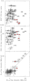 |
Fig. 13 Comparison of molecular line intensities and tracers of SF. The bottom panel compares the SFR tracers: background-subtracted 24 μm emission and 8 μm emission, also background-subtracted (the background emission is considerably stronger than any stellar contribution at 8 μm). The middle panel shows how the 12CO intensity varies with SFR. The top panel shows how the dense gas fraction, as traced by the HCO+/CO ratio, varies with SFR. The red triangles indicate the sources which are at high Galactic latitude. It should be immediately apparent that these sources are not distinguishable from the others in the lower two frames but occupy a specific region with low dense gas fraction in the top panel. Neither 8 nor 24 μm data are available for cloud 30. |
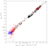 |
Fig. 14 Link between dense gas mass (HCN or HCO+ luminosity on the x-axis) and SF rate (IR luminosity on the y-axis). The line shows a linear relation with |

7 Comparison with other environments
In the extreme outer Galaxy clouds observed here, the line intensity ratios are approximately: CO/HCN ~ 70, CO/HCO+ ~ 35, and CO/13CO ~ 7.5. Thus, the CO emission is stronger relative to the other lines than in the majority of sources observed thus far (see e.g., Fig. 8 of Chen et al. 2015).
However, in the nearly square degree region of Orion B mapped by Gratier et al. (2017), they obtain very similar ratios for their median values of CO,13 CO, HCO+, and HCN, although the HCN emission is stronger after correction for flux in the satellite lines. The median values tend to sample the more extended lower column density regions, as also found recently by Evans et al. (2020).
The Shimajiri et al. (2017) work on nearby molecular clouds showed that HCN and HCO+ emission often traced SF while the H13CN and H13CO+ lines were sensitive to the total H2 column. These regions are much denser than the outer Galaxy clouds studied here and the HCN and HCO+ emission is highly optically thick. The net effect is that the intensity of HCN and HCO+ is highly dependent on gas temperature (thus SF) rather than density. In the highest column density regions, the main isotope lines are strongly self-absorbed. HCN emission in outer Milky Way clouds is optically thin and does not trace SF and so it appears akin to the H13CN in Shimajiri et al. (2017), which traces column density in high volume density regions. While Shimajiri et al. (2017) do not calculate H13CN abundances, the H13CO+ abundances are within a rather narrow range: 1.5–5.8 × 10⁻¹¹ with respect to H2. These values are consistent with  and the column densities (
 ) are similar to our estimates for the main isotope.
Yuan et al. (2016) present HCN and HCO+ observations, also with the PMO telescope, of cool clumps identified by the Planck satellite. They are at approximately the solar circle (mean distance of 1.3 kpc). Their estimated column densities are variable but have median NHCN and  , although the ratio is quite variable. Their abundance estimates differ from source to source but are mostly χ ~ 10−10 for both HCN and HCO+. Other Galactic works include Park et al. (1999) and Barnes et al. (2011) who assume higher abundances, typically χ ~ 10−9. In the cool clouds, the HCO+ line is stronger than HCN.
So far we have compared with other Galactic observations but extragalactic sources allow for a much greater range in properties. A relatively distant region in M 51 was observed with the IRAM interferometer by Chen et al. (2017) who found HCN/CO ratios similar to ours but generally higher HCN/HCO+ ratios. M 31 was observed by Brouillet et al. (2005) and, in the outer parts, a similarly low HCN/CO ratio was found but again a higher HCN/HCO+ ratio. The Large Magellanic Cloud (LMC) provides an environment with a lower metallicity and a higher radiation field than our observations of the outer Milky Way but at similar scales. Chin et al. (1997) observed several lines in the LMC and found again that the HCO+ emission was stronger than the HCN (or HNC), unlike large Milky Way molecular clouds or star-forming galaxies (their Table 10). Subsequently, Nishimura et al. (2016), Anderson et al. (2014), Galametz et al. (2020), and Seale et al. (2012) observed CO-strong molecular clouds in the LMC and consistently confirm the weak emission from nitrogen-bearing molecules, as well as strong CCH emission. Braine et al. (2017) observed the low-metallicity galaxies M 33, IC 10, and NGC 6822 in the local group and found ratios quite similar to those presented here. These authors concluded that the low HCN/HCO+ ratio was due to weak HCN emission rather than particularly strong HCO+ emission. This was attributed to the decrease in N/O with metal deficiency.
The low HCN/HCO+ ratios we observe in the extreme outer Galaxy are probably due to a combination of low volume density and subsolar metallicity. A gradient in N/O exists in the Galaxy (Magrini et al. 2018). However, while Arellano-Cordova et al. (2021) find a N/O gradient of −0.015 dex kpc−1 from optical observations, Rudolph et al. (2006) find a N/O gradient of −0.03 dex kpc−1 from far-IR spectral line data. As a result, the N/O ratio for the distant clouds should be approximately half of the solar circle value. If the new values underestimate the gradient, then the low HCN fluxes could be entirely due to a decrease in abundance. Two features lead us to believe that volume density is also an issue. First of all, the new gradient uses high-quality Gaia DR2 distances. Secondly, the low molecular fraction in and the diffuse nature of the outer parts of spiral galaxies argues for a lower hydrostatic pressure as compared to the inner disk (see e.g., Blitz & Rosolowsky 2004). While the molecular line ratios are not clearly related to the level of SF, there is a clear difference between the clouds in the plane and those at b > 2° in that the HCO+/CO ratio is lower for the latter (Fig. 13, but also HCO+/13CO and the same ratios with HCN). Our clouds at higher latitude are at h ≳ 300 pc from the Galactic plane such that the local pressure should be lower.
We find a similar effect in the Yuan et al. (2016) sample. Clouds with h > 180pc above the plane have significantly lower average and median  and IHCN/(N13CO) values than the clouds at h < 180pc. The mean values are 50% higher in the plane and the median is twice as high for both
  and IHCN/(N13CO). (N13CO) has been used as the reference column density but the higher dense fraction (stronger HCN and HCO+ emission) close to the Galactic plane is equally found using the 12CO column density (see Table 3 of Yuan et al. 2016).
8 Conclusions
The dense gas tracers HCN(1−0) and HCO+(1−0) were observed in a sample of extreme outer Galaxy clouds (15 ≳ Rgal ≲ 21 kpc) from the Sun et al. (2015) unbiased CO survey. The clouds were chosen for their reasonably strong CO (ICO > 7 km s−1) and  emission. None were detected in C18O(1−0); however, the limits are close to what would be expected for optically thin emission so far out in the disk.
The HCN and HCO+ emission is weak, both in an absolute sense and relative to the CO lines (Tables 1 and 2). The line ratios follow approximately
 after accounting for the satellite HCN lines. These ratios are typical of a subsolar metallicity environment, where N is more affected than O.
The 12CO(1−0) emission is highly optically thick, but the 13CO(1−0) is optically thin, τ13 ≲ 1. The estimated H2 column densities are ~1022 cm−2, depending on the hypotheses (Table 3), but in all cases they are several times higher than would be deduced from a standard extragalactic N (H2)/ICO ~ 2 × 1020cm−2/(K km s−1) conversion factor (e.g., Bolatto et al. 2013).
The lines are narrow and the hyperfine ratios of HCN indicate that the emission is optically thin, τΗCN(1−0) ≲ 1. We obtain beam-averaged HCN column densities, for our fiducial excitation temperature, of 1–7 × 1011 cm−2 (Table 3, Col. 10). With the optical depths, we can estimate the dense gas filling factor, again dependent on the assumed Tex, and we obtain values of 10 ± 6% (Table 3), which is in reasonable agreement with other estimates. Other molecules and transitions can trace gas substantially denser, which would then have a lower filling factor. Similar results are obtained for the HCO+ line (see Table 1).
The H2 volume densities required to collisionally excite the optically thin HCN and HCO+ lines are about 100 times those required to excite the CO lines. As explained in Sect. 4.5, we conclude that the HCN and HCO+ emission does not trace the dominant mass component of the gas but the denser clumps. Combined with the derived filling factors, and dependent on the assumed but poorly known abundances of HCN and HCO+, we estimate (Sect. 4.5) that the gas emitting the HCN(1−0) and HCO+(1−0) flux represents some 10% of the total gas mass.
The critical densities of HCN and HCO+ are not the same and we used RADEX non-LTE models to obtain estimates of the HCN column density and we used the HCN/HCO+ intensity ratio to constrain the volume density of the “dense” gas. Because these lines are optically thin, the intensity ratio depends on the abundance ratio. For
 (Watanabe et al. 2017), the “dense” gas is likely n(H2) ≲ 104 cm−3; however, if the relative HCO+ abundance is higher, as obtained in Sect. 4, then denser gas is required for the same line ratio.
As part of the modeling, it was realized that the high cross-F rates initially found by Ben Abdallah et al. (2012) could not fit our data, but that the revised rates by Hernández Vera et al. (2017) provided a good fit. It was thus possible to observationally test hyperfine collision rates.
The original motivation was to explore the link between star formation and dense gas in the poorly known outer disk environment. Our data fall on the general LHCN–LIR plot (Fig. 14); however, within our sample, there is no correlation between the SFR, as traced by the 8μm and/or 24 μm flux, and the flux in the HCN and HCO+ lines or the dense gas fraction as traced by the HCN/CO or HCO+/CO line ratios. Instead, we find that the dense gas fraction decreases away from the Galactic plane, presumably due to lower pressure. An analysis of the Yuan et al. (2016) sources reveals the same trend.
The clouds observed here are extreme outer Galaxy clouds (15–21 kpc from the Galactic center). Although the HCN emission is weak, it is optically thin so the optical depth and column density can be estimated from the hyperfine ratios. Both dense gas tracers (HCN and HCO+) are weak in the clouds further than 300pc from the Galactic plane, suggesting that the lower pressure far from the plane leads to a lower dense gas fraction.
More observations of “ordinary” outer Galaxy clouds are clearly necessary to see if the trend with distance from the plane can be refined and, perhaps, clearly associated with local pressure. Further measurements of HCN and HCO+ in nearby galaxies near or beyond the optical radius, coupled with optical abundance measurements, should separate density and abundance effects to explain the decrease in the HCN/HCO+ intensity ratio with galactocentric distance.
Acknowledgements
We would like to dedicate this work to our dear friend and colleague Prof. Yu Gao, who passed away during the revision of the article. We would like to thank the DeLingHa telescope staff and the Purple Mountain Observatory for making these observations possible. JB would like to thank NanJing University for hosting. We would also like to ackowledge grants from the french PNGC and the ANR program for financing through the ANR-11-BS56-010 project STARFICH. Y.S. acknowledges support by the Youth Innovation Promotion Association, CAS (Y2022085), Light of West China Program, CAS (No. xbzg-zdsys-202212), and the NSFC through grant 11773077. H.C. is supported by Key Research Project of Zhejiang Lab No. 2021PE0AC0. Y.G. research was supported by the National Key Basic Research and Development Program of China (2017YFA0402700), the National Natural Science Foundation of China (11861131007, U1731237, 12033004), and Chinese Academy of Sciences Key Research Program of Frontier Sciences (QYZDJSSW-SLH008). This publication makes use of data products from the Wide-field Infrared Survey Explorer, which is a joint project of the University of California, Los Angeles, and the Jet Propulsion Laboratory/California Institute of Technology, funded by the National Aeronautics and Space Administration.
References
- Aladro, R., Martín, S., Martín-Pintado, J., et al. 2011, A & A, 535, A84 [NASA ADS] [CrossRef] [EDP Sciences] [Google Scholar]
- Anderson, C. N., Meier, D. S., Ott, J., et al. 2014, ApJ, 793, 37 [CrossRef] [Google Scholar]
- Arellano-Córdova, K. Z., Esteban, C., García-Rojas, J., & Méndez-Delgado, J. E. 2021, MNRAS, 502, 225 [CrossRef] [Google Scholar]
- Barnes, P. J., Yonekura, Y., Fukui, Y., et al. 2011, ApJS, 196, 12 [NASA ADS] [CrossRef] [Google Scholar]
- Ben Abdallah, D., Najar, F., Jaidane, N., Dumouchel, F., & Lique, F. 2012, MNRAS, 419, 2441 [NASA ADS] [CrossRef] [Google Scholar]
- Binney, J., & Vasiliev, E. 2023, MNRAS, 520, 1832 [NASA ADS] [CrossRef] [Google Scholar]
- Blitz, L., & Rosolowsky, E. 2004, ApJ, 612, L29 [NASA ADS] [CrossRef] [Google Scholar]
- Bolatto, A. D., Wolfire, M., & Leroy, A. K. 2013, ARA & A, 51, 207 [NASA ADS] [CrossRef] [Google Scholar]
- Boquien, M., Calzetti, D., Kramer, C., et al. 2010, A & A, 518, A70 [Google Scholar]
- Boquien, M., Calzetti, D., Aalto, S., et al. 2015, A & A, 578, A8 [NASA ADS] [CrossRef] [EDP Sciences] [Google Scholar]
- Bovy, J., & Rix, H.-W. 2013, ApJ, 779, 115 [Google Scholar]
- Braine, J., Combes, F., & van Driel, W. 1993, A & A, 280, 451 [NASA ADS] [Google Scholar]
- Braine, J., Shimajiri, Y., André, P., et al. 2017, A & A, 597, A44 [NASA ADS] [CrossRef] [EDP Sciences] [Google Scholar]
- Brouillet, N., Muller, S., Herpin, F., Braine, J., & Jacq, T. 2005, A & A, 429, 153 [NASA ADS] [CrossRef] [EDP Sciences] [Google Scholar]
- Buchbender, C. 2014, PhD thesis, Universidad de Granada, Spain http://hdl.handle.net/10481/31707 [Google Scholar]
- Calzetti, D., Kennicutt, R. C., Engelbracht, C. W., et al. 2007, ApJ, 666, 870 [Google Scholar]
- Chen, H., Gao, Y., Braine, J., & Gu, Q. 2015, ApJ, 810, 140 [NASA ADS] [CrossRef] [Google Scholar]
- Chen, H., Braine, J., Gao, Y., Koda, J., & Gu, Q. 2017, ApJ, 836, 101 [NASA ADS] [CrossRef] [Google Scholar]
- Chin, Y.-N., Henkel, C., Whiteoak, J. B., et al. 1997, A & A, 317, 548 [NASA ADS] [Google Scholar]
- Chin, Y.-N., Henkel, C., Millar, T. J., Whiteoak, J. B., & Marx-Zimmer, M. 1998, A & A, 330, 901 [NASA ADS] [Google Scholar]
- Digel, S., de Geus, E., & Thaddeus, P. 1994, ApJ, 422, 92 [NASA ADS] [CrossRef] [Google Scholar]
- Draine, B. T., Dale, D. A., Bendo, G., et al. 2007, ApJ, 663, 866 [NASA ADS] [CrossRef] [Google Scholar]
- Evans, Neal J. I., 1999, ARA & A, 37, 311 [NASA ADS] [CrossRef] [Google Scholar]
- Evans, Neal J. I., Kim K.-T., Wu, J., et al. 2020, ApJ, 894, 103 [NASA ADS] [CrossRef] [Google Scholar]
- Fang, M., Kim, J. S., van Boekel, R., et al. 2013, ApJS, 207, 5 [NASA ADS] [CrossRef] [Google Scholar]
- Flower, D. R. 1999, MNRAS, 305, 651 [Google Scholar]
- Fontani, F., Giannetti, A., Beltrán, M. T., et al. 2012, MNRAS, 423, 2342 [NASA ADS] [CrossRef] [Google Scholar]
- Fontani, F., Colzi, L., Bizzocchi, L., et al. 2022, A & A, 660, A76 [NASA ADS] [CrossRef] [EDP Sciences] [Google Scholar]
- Freeman, K. C. 1970, ApJ, 160, 811 [Google Scholar]
- Galametz, M., Kennicutt, R. C., Calzetti, D., et al. 2013, MNRAS, 431, 1956 [NASA ADS] [CrossRef] [Google Scholar]
- Galametz, M., Schruba, A., De Breuck, C., et al. 2020, A & A, 643, A63 [NASA ADS] [CrossRef] [EDP Sciences] [Google Scholar]
- Gallagher, M. J., Leroy, A. K., Bigiel, F., et al. 2018, ApJ, 858, 90 [NASA ADS] [CrossRef] [Google Scholar]
- Gao, Y., & Solomon, P. M. 2004a, ApJS, 152, 63 [Google Scholar]
- Gao, Y., & Solomon, P. M. 2004b, ApJ, 606, 271 [NASA ADS] [CrossRef] [Google Scholar]
- Gao, Y., Carilli, C. L., Solomon, P. M., & Vanden Bout, P. A. 2007, ApJ, 660, L93 [NASA ADS] [CrossRef] [Google Scholar]
- García-Burillo, S., Usero, A., Alonso-Herrero, A., et al. 2012, A & A, 539, A8 [CrossRef] [EDP Sciences] [Google Scholar]
- Glover, S. C. O., & Clark, P. C. 2012, MNRAS, 426, 377 [Google Scholar]
- Godard, B., Falgarone, E., Gerin, M., Hily-Blant, P., & de Luca, M. 2010, A & A, 520, A20 [NASA ADS] [CrossRef] [EDP Sciences] [Google Scholar]
- Graciá-Carpio, J., García-Burillo, S., Planesas, P., Fuente, A., & Usero, A. 2008, A & A, 479, 703 [CrossRef] [EDP Sciences] [Google Scholar]
- Gratier, P., Bron, E., Gerin, M., et al. 2017, A & A, 599, A100 [NASA ADS] [CrossRef] [EDP Sciences] [Google Scholar]
- Green, S., & Thaddeus, P. 1974, ApJ, 191, 653 [Google Scholar]
- Guilloteau, S., & Baudry, A. 1981, A & A, 97, 213 [NASA ADS] [Google Scholar]
- Gusev, A. S., Guslyakova, S. A., & Khramtsova, M. S. 2012, Astron. Astrophys. Trans., 27, 233 [NASA ADS] [Google Scholar]
- Hernández Vera, M., Lique, F., Dumouchel, F., Hily-Blant, P., & Faure, A. 2017, MNRAS, 468, 1084 [Google Scholar]
- Hoekstra, H., van Albada, T. S., & Sancisi, R. 2001, MNRAS, 323, 453 [NASA ADS] [CrossRef] [Google Scholar]
- Jiménez-Donaire, M. J., Bigiel, F., Leroy, A. K., et al. 2019, ApJ, 880, 127 [CrossRef] [Google Scholar]
- Juneau, S., Narayanan, D. T., Moustakas, J., et al. 2009, ApJ, 707, 1217 [NASA ADS] [CrossRef] [Google Scholar]
- Kalberla, P. M. W., & Kerp, J. 2009, ARA & A, 47, 27 [NASA ADS] [CrossRef] [Google Scholar]
- Kennicutt, R. C. J. 1989, ApJ, 344, 685 [CrossRef] [Google Scholar]
- Kennicutt, R. C., & Evans, N. J. 2012, ARA & A, 50, 531 [NASA ADS] [CrossRef] [Google Scholar]
- Kepley, A. A., Leroy, A. K., Frayer, D., et al. 2014, ApJ, 780, L13 [Google Scholar]
- Koenig, X. P., Leisawitz, D. T., Benford, D. J., et al. 2012, ApJ, 744, 130 [Google Scholar]
- Krips, M., Neri, R., García-Burillo, S., et al. 2008, ApJ, 677, 262 [NASA ADS] [CrossRef] [Google Scholar]
- Kutner, M. L., & Ulich, B. L. 1981, ApJ, 250, 341 [NASA ADS] [CrossRef] [Google Scholar]
- Kwan, J., & Scoville, N. 1975, ApJ, 195, L85 [NASA ADS] [CrossRef] [Google Scholar]
- Lahuis, F., & van Dishoeck, E. F. 2000, A & A, 355, 699 [NASA ADS] [Google Scholar]
- Linsky, J. L. 2003, Space Sci. Rev., 106, 49 [Google Scholar]
- Ma, B., Tan, J. C., & Barnes, P. J. 2013, ApJ, 779, 79 [Google Scholar]
- Magrini, L., Vincenzo, F., Randich, S., et al. 2018, A & A, 618, A102 [NASA ADS] [CrossRef] [EDP Sciences] [Google Scholar]
- Mangum, J. G., & Shirley, Y. L. 2015, PASP, 127, 266 [Google Scholar]
- Martín, S., Mauersberger, R., Martín-Pintado, J., Henkel, C., & García-Burillo, S. 2006, ApJS, 164, 450 [Google Scholar]
- Molinari, S., Schisano, E., Elia, D., et al. 2016, A & A, 591, A149 [NASA ADS] [CrossRef] [EDP Sciences] [Google Scholar]
- Müller, H. S. P., Schlöder, F., Stutzki, J., & Winnewisser, G. 2005, J. Mol. Struct., 742, 215 [Google Scholar]
- Nishimura, Y., Shimonishi, T., Watanabe, Y., et al. 2016, ApJ, 818, 161 [NASA ADS] [CrossRef] [Google Scholar]
- Nishimura, Y., Watanabe, Y., Harada, N., et al. 2017, ApJ, 848, 17 [NASA ADS] [CrossRef] [Google Scholar]
- Park, Y. S., Kim, J., & Minh, Y. C. 1999, ApJ, 520, 223 [NASA ADS] [CrossRef] [Google Scholar]
- Patra, S., Evans, Neal J. I., Kim, K.-T., et al. 2022, AJ, 164, 129 [NASA ADS] [CrossRef] [Google Scholar]
- Pedicelli, S., Bono, G., Lemasle, B., et al. 2009, A & A, 504, 81 [NASA ADS] [CrossRef] [EDP Sciences] [Google Scholar]
- Pineda, J. L., Langer, W. D., Velusamy, T., & Goldsmith, P. F. 2013, A & A, 554, A103 [NASA ADS] [CrossRef] [EDP Sciences] [Google Scholar]
- Pirogov, L., Zinchenko, I., Lapinov, A., Myshenko, V., & Shul’Ga, V. 1995, A & AS, 109, 333 [NASA ADS] [Google Scholar]
- Privon, G. C., Herrero-Illana, R., Evans, A. S., et al. 2015, ApJ, 814, 39 [CrossRef] [Google Scholar]
- Ragan, S. E., Henning, T., Tackenberg, J., et al. 2014, A & A, 568, A73 [NASA ADS] [CrossRef] [EDP Sciences] [Google Scholar]
- Reid, M. J., Menten, K. M., Brunthaler, A., et al. 2014, ApJ, 783, 130 [Google Scholar]
- Rudolph, A. L., Fich, M., Bell, G. R., et al. 2006, ApJS, 162, 346 [Google Scholar]
- Sakamoto, S., Hasegawa, T., Handa, T., Hayashi, M., & Oka, T. 1997, ApJ, 486, 276 [NASA ADS] [CrossRef] [Google Scholar]
- Sandstrom, K. M., Leroy, A. K., Walter, F., et al. 2013, ApJ, 777, 5 [Google Scholar]
- Schmidt, T. M., Bigiel, F., Klessen, R. S., & de Blok, W. J. G. 2016, MNRAS, 457, 2642 [NASA ADS] [CrossRef] [Google Scholar]
- Schöier, F. L., van der Tak, F. F. S., van Dishoeck, E. F., & Black, J. H. 2005, A & A, 432, 369 [CrossRef] [EDP Sciences] [Google Scholar]
- Schuller, F., Menten, K. M., Contreras, Y., et al. 2009, A & A, 504, 415 [NASA ADS] [CrossRef] [EDP Sciences] [Google Scholar]
- Seale, J. P., Looney, L. W., Wong, T., et al. 2012, ApJ, 751, 42 [NASA ADS] [CrossRef] [Google Scholar]
- Shan, W. L., Yang, J., & Shi, S. C., et al. 2012, ITTST, 2, 593 [NASA ADS] [Google Scholar]
- Shimajiri, Y., André, P., Braine, J., et al. 2017, A & A, 604, A74 [NASA ADS] [CrossRef] [EDP Sciences] [Google Scholar]
- Shirley, Y. L. 2015, PASP, 127, 299 [Google Scholar]
- Skrutskie, M. F., Cutri, R. M., Stiening, R., et al. 2006, AJ, 131, 1163 [NASA ADS] [CrossRef] [Google Scholar]
- Sodroski, T. J., Odegard, N., Dwek, E., et al. 1995, ApJ, 452, 262 [Google Scholar]
- Sodroski, T. J., Odegard, N., Arendt, R. G., et al. 1997, ApJ, 480, 173 [NASA ADS] [CrossRef] [Google Scholar]
- Sun, Y. 2015, PhD thesis, Purple Mountain Observatory, Chinese Academy of Sciences PR China [Google Scholar]
- Sun, Y., Xu, Y., Yang, J., et al. 2015, ApJ, 798, L27 [Google Scholar]
- Turner, B. E., Pirogov, L., & Minh, Y. C. 1997, ApJ, 483, 235 [CrossRef] [Google Scholar]
- Usero, A., Leroy, A. K., Walter, F., et al. 2015, AJ, 150, 115 [Google Scholar]
- van der Tak, F. F. S., Black, J. H., Schöier, F. L., Jansen, D. J., & van Dishoeck, E. F. 2007, A & A, 468, 627 [NASA ADS] [CrossRef] [EDP Sciences] [Google Scholar]
- Wang, Y., Beuther, H., Schneider, N., et al. 2020, A & A, 641, A53 [CrossRef] [EDP Sciences] [Google Scholar]
- Watanabe, Y., Sakai, N., Lindberg, J. E., et al. 2012, ApJ, 745, 126 [NASA ADS] [CrossRef] [Google Scholar]
- Watanabe, Y., Sakai, N., Sorai, K., & Yamamoto, S. 2014, ApJ, 788, 4 [NASA ADS] [CrossRef] [Google Scholar]
- Watanabe, Y., Nishimura, Y., Harada, N., et al. 2017, ApJ, 845, 116 [Google Scholar]
- Wouterloot, J. G. A., & Brand, J. 1989, A & AS, 80, 149 [NASA ADS] [Google Scholar]
- Wright, E. L., Eisenhardt, P. R. M., Mainzer, A. K., et al. 2010, AJ, 140, 1868 [Google Scholar]
- Wu, J., Evans, N. J.II, Gao, Y., et al. 2005, ApJ, 635, L173 [NASA ADS] [CrossRef] [Google Scholar]
- Wu, J., Evans, N. J.II, Shirley, Y. L., & Knez, C. 2010, ApJS, 188, 313 [NASA ADS] [CrossRef] [Google Scholar]
- Yuan, J., Wu, Y., Liu, T., et al. 2016, ApJ, 820, 37 [NASA ADS] [CrossRef] [Google Scholar]
Estimates of the disk mass scale length of the Galaxy range between 2 and 3 kpc (Binney & Vasiliev 2023; Bovy & Rix 2013) and following Gusev et al. (2012) we estimate the blue-band scale length to be about 3.5 kpc, yielding R25 ≈ 11 kpc assuming a central disk surface brightness of 21.65 mag/″2 from Freeman (1970).
All Tables
All Figures
|
Fig. 1 WISE 22 μm band images of sources 7, 14, 16, 18, 30, and 34 (identification in upper right corner). These are the sources for which only a single pointing is available. The images are all 10 arcmin in size, oriented in l and b. The central circle gives the HCN/HCO+ beamsize. The transfer function (rainbow from black to white) of the WISE observations differs from image to image. For cloud 7 it is from 91.5 to 98; for cloud 14 it is 100.5 to 107; for 16 it is 103 to 115; for 18 it is 102 to 114; for 30 it is from 108 to 112 and for cloud 34 it is from 108 to 135 counts. Following Sun (2015), class I sources within our maps are shown as circles and class II as squares. |
| In the text | |
|
Fig. 2 WISE 22 μm band images of sources 21, 56, and 57 (identification in upper right corner). These are the sources which were mapped. The images are all 600″ × 400″ in size, oriented in l and b. The color scale (rainbow from black to white) of the WISE observations differs from image to image. For cloud 21 it is from 95 to 116 and for clouds 56 and 57 the range is from 129 to 134 counts. The central circle gives the HCN/HCO+ beamsize and is the (0,0) position in Figs. 4–6 which show the spectra. The box indicates the size of the region shown in Figs. 4–6. Following Sun (2015), class I sources within our maps are shown as circles and class II as squares. |
| In the text | |
|
Fig. 3 Spectra for the clouds that have not been mapped, as in Fig. 1. The axes are the same for each cloud. 12CO is in black and corresponds to the temperature scale. 13CO is in red and has been multiplied by 5. HCO+, in green, has been multiplied by 35. The HCN spectra have been multiplied by 35 for comparison with HCO+ but also multiplied by 9/5 to account for the satellite lines as explained in the text. The 12CO and 13CO spectra have been convolved with a Gaussian kernel to the angular resolution of the HCN and HCO+ spectra. |
| In the text | |
|
Fig. 4 Spectra of Cloud 21. Positions are indicated on the x and y axes as offsets in arcminutes and each box represents 30″. 12CO is in black, 13CO in red, HCO+ in green and HCN in blue. The velocity scale goes from −106.5 km s−1 to −97 km s−1. The temperatures scales are −.7 to 7 K for 12CO, −.14 to −1.4 K for 13CO, −.02 to .2 for HCO+ and for HCN. The HCN line (only central component shown) has been multiplied by 9/5 so that the line intensity represents the total line flux for comparison with other species. The 12CO and 13CO spectra have been convolved to the same angular resolution as the HCN and HCO+. |
| In the text | |
|
Fig. 5 Spectra of Cloud 56. Positions are indicated on the x and y axes as offsets in arcminutes and each box represents 30″. 12CO is in black, 13CO in red, HCO+ in green and HCN in blue. The velocity scale goes from −107.5 km s−1 to −99 km s−1. The temperatures scales are −.7 to 7K for 12CO, −.14 to 1.4K for 13CO, −.02 to .2 for HCO+ and for HCN. The HCN line (only central component shown) has been multiplied by 9/5 so that the line intensity represents the total line flux for comparison with other species. The spectra in the corners show only CO as not all positions were observed in HCN and HCO+. |
| In the text | |
|
Fig. 6 Spectra of Cloud 57. Positions are indicated on the x and y axes as offsets in arcminutes and each box represents 30″. 12CO is in black, 13CO in red, HCO+ in green and HCN in blue. The velocity scale goes from −106.5 km s−1 to −98 km s−1. The temperatures scales are −.7 to 7 K for 12CO, −.14 to 1.4 K for 13CO, −.02 to .2 for HCO+ and for HCN. The HCN line (only central component shown) has been multiplied by 9/5 so that the line intensity represents the total line flux for comparison with other species. The spectra in the corners show only CO as not all positions were observed in HCN and HCO+. |
| In the text | |
|
Fig. 7 Sum of spectra for each of the clouds for which we were able to make maps. The lines are narrow although each spectrum represents a sum of many positions. The clear separation of the hyperfine components enables us to estimate the optical depth. The parameters of the Gaussian fits shown in green are given in Table 2. |
| In the text | |
|
Fig. 8 Integrated intensities of HCN and HCO+ lines for all positions observed. All data are on the main beam temperature scale and the central HCN intensity has been multiplied by 9/5 to account for the satellite hyperfine components. The line indicates |
| In the text | |
|
Fig. 9 Integrated intensities of 12CO and 13CO lines for all positions observed. The line indicates the best-fit: |
| In the text | |
|
Fig. 10 LTE representation of hyperfine component ratios as a function of main component (F = 2−1) optical depth. The observed ratios for clouds 21, 56, and 57 are indicated. The vertical dashed lines indicate the uncertainties from Table 3. |
| In the text | |
|
Fig. 11 Intensity ratios of the hyperfine components of the HCN J = 1−0 line, calculated with RADEX as a function of N(HCN). Gray areas indicate observed ranges for the F = 1−1/2−1 (top) and 0−1/2−1 (bottom) ratios, respectively 0.6, 0.6, 0.7 and 0.2, 0.2, 0.3 for clouds 21, 56, and 57. The numbers indicating the rates refer to the years of publication of the rates. |
| In the text | |
|
Fig. 12 Intensity ratio of the HCN and HCO+ J = 1−0 lines, calculated with RADEX as a function of n(H2). |
| In the text | |
|
Fig. 13 Comparison of molecular line intensities and tracers of SF. The bottom panel compares the SFR tracers: background-subtracted 24 μm emission and 8 μm emission, also background-subtracted (the background emission is considerably stronger than any stellar contribution at 8 μm). The middle panel shows how the 12CO intensity varies with SFR. The top panel shows how the dense gas fraction, as traced by the HCO+/CO ratio, varies with SFR. The red triangles indicate the sources which are at high Galactic latitude. It should be immediately apparent that these sources are not distinguishable from the others in the lower two frames but occupy a specific region with low dense gas fraction in the top panel. Neither 8 nor 24 μm data are available for cloud 30. |
| In the text | |
|
Fig. 14 Link between dense gas mass (HCN or HCO+ luminosity on the x-axis) and SF rate (IR luminosity on the y-axis). The line shows a linear relation with |
| In the text | |
Current usage metrics show cumulative count of Article Views (full-text article views including HTML views, PDF and ePub downloads, according to the available data) and Abstracts Views on Vision4Press platform.
Data correspond to usage on the plateform after 2015. The current usage metrics is available 48-96 hours after online publication and is updated daily on week days.
Initial download of the metrics may take a while.