| Issue |
A&A
Volume 675, July 2023
|
|
|---|---|---|
| Article Number | A163 | |
| Number of page(s) | 20 | |
| Section | Extragalactic astronomy | |
| DOI | https://doi.org/10.1051/0004-6361/202345844 | |
| Published online | 14 July 2023 | |
Expectations for time-delay measurements in active galactic nuclei with the Vera Rubin Observatory⋆
1
Center for Theoretical Physics, Polish Academy of Sciences, Al. Lotników 32/46, 02-668 Warsaw, Poland
e-mail: This email address is being protected from spambots. You need JavaScript enabled to view it.
2
Laboratório Nacional de Astrofísica – MCTI, R. dos Estados Unidos, 154 - Nações, Itajubá, MG 37504-364, Brazil
3
Department of Theoretical Physics and Astrophysics, Faculty of Science, Masaryk University, Kotlarska 2, 61137 Brno, Czech Republic
4
Departamento de Astronomia, Universidad de Chile, Camino del Observatorio 1515, Santiago, Casilla 36-D, Chile
5
Astronomical Observatory, University of Warsaw, Al.Ujazdowskie 4, 00-478 Warszawa, Poland
6
University of Belgrade-Faculty of Mathematics, Department of astronomy, Studentski trg 16, Belgrade, Serbia
7
Humboldt Research Fellow, Hamburger Sternwarte, Universität Hamburg, Gojenbergsweg 112, 21029 Hamburg, Germany
8
Astronomical Observatory, Volgina 7, 11160 Belgrade, Serbia
9
Astroinformatics, Heidelberg Institute for Theoretical Studies, Schloss-Wolfsbrunnenweg 35, 69118 Heidelberg, Germany
10
School of Physics & Astronomy, University of Southampton, Southampton SO17 1BJ, UK
11
Department of Astronomy and Astrophysics, 525 Davey Lab, The Pennsylvania State University, University Park, PA 16802, USA
Received:
4
January
2023
Accepted:
6
June
2023
Abstract
Context. The Vera Rubin Observatory will provide an unprecedented set of time-dependent observations of the sky. The planned Legacy Survey of Space and Time (LSST), operating for ten years, will provide dense light curves for thousands of active galactic nuclei (AGN) in deep drilling fields (DDFs) and less dense light curves for millions of AGN from the main survey (MS).
Aims. We model the prospects for measuring the time delays for the AGN emission lines with respect to the continuum, using these data.
Methods. We modeled the artificial light curves using the Timmer-König algorithm. We used the exemplary cadence to sample them (one for the MS and one for the DDF), we supplement light curves with the expected contamination by the strong emission lines (Hβ, Mg II, and CIV, as well as with Fe II pseudo-continuum and the starlight). We chose suitable photometric bands that are appropriate for the redshift and compared the assumed line time-delay with the recovered time delay for 100 statistical realizations of the light curves.
Results. We show that time delays for emission lines can be well measured from the main survey for the bright tail of the quasar distribution (about 15% of all sources) with an accuracy within 1σ error. For the DDF, the results for fainter quasars are also reliable when the entire ten years of data are used. There are also some prospects to measure the time delays for the faintest quasars at the lowest redshifts from the first two years of data, and possibly even from the first season. The entire quasar population will allow us to obtain results of apparently high accuracy, but in our simulations, we see a systematic offset between the assumed and recovered time delay that depends on the redshift and source luminosity. This offset will not disappear even in the case of large statistics. This problem might affect the slope of the radius-luminosity relation and cosmological applications of quasars if no simulations are performed that correct for these effects.
Key words: galaxies: active / quasars: emission lines / quasars: supermassive black holes
On behalf of the LSST-AGN Science Collaboration.
CNPq Fellow.
© The Authors 2023
 Open Access article, published by EDP Sciences, under the terms of the Creative Commons Attribution License (https://creativecommons.org/licenses/by/4.0), which permits unrestricted use, distribution, and reproduction in any medium, provided the original work is properly cited.
This article is published in open access under the Subscribe to Open model. This email address is being protected from spambots. You need JavaScript enabled to view it. to support open access publication.
1. Introduction
The Vera C. Rubin Observatory and its Legacy Survey of Space and Time (LSST; Ivezić et al. 2019) will provide an unprecedented amount of data in many fields and will thus revolutionize our view of the Universe. Observations will start relatively soon, most likely in mid-2024. Optimizing the output from these data, particularly from the first stages of its operation, is therefore extremely important. Among numerous results, LSST will provide up to ten million quasars. This will open a path to massive reverberation monitoring of active galactic nuclei (AGN) in a range of redshifts from 0 up to 7 (Shen et al. 2020; Kovačević et al. 2021).
The current description of the Vera Rubin Observatory can be found in Ivezić et al. (2019). General expectations of the LSST discoveries in the field of AGN were discussed by Brandt et al. (2018), and specific predictions for the mapping of AGN accretion disks with the LSST were presented by Kovačević et al. (2022) and Pozo Nuñez et al. (2023). The prospects for the continuum time-delays from accretion disks were also discussed by Yu et al. (2020). In the current paper, we aim to assess the accuracy with which emission-line time delays can be measured using the four photometric bands of the LSST. Broad emission lines are characteristic for almost all bright AGN (see, e.g., Krolik 1999, for a suitable review). The exact location and geometry of the corresponding region (known as the broadline region, BLR) is generally unresolved, except for the most recent observations of three AGN in the infrared domain with the use of the GRAVITY Very Large Telescope Interferometer (VLTI) (3C 273; GRAVITY Collaboration 2018, NGC 3783; GRAVITY Collaboration 2021, and IRAS 09149-6206; GRAVITY Collaboration 2020). For the remaining objects, we rely on reverberation monitoring in order to understand the structure and dynamics of their BLRs.
Reverberation mapping is a well-established observational technique that has been extensively used to study the inner structure of AGN on subparsec length scales, which are typically beyond the resolution limits of current telescopes. It effectively replaces the spatial resolution with a time resolution that needs to be adjusted according to the spatial scale of interest (see, e.g., Cackett et al. 2021, for a review and references therein). The idea was proposed in 1982 by Blandford & McKee (1982), who showed that the line emission produced in the BLR follows the same variability pattern as the continuum emission from the disk, but is delayed by the light travel time between the disk and the BLR. The first systematic observational results were published in 1990–1993, presenting the results from the ground-based campaigns as well as from the International Ultraviolet Explorer (IUE) for the bright nearby AGN (Maoz et al. 1990; Netzer & Maoz 1990; Peterson & Gaskell 1991; Peterson et al. 1991; Peterson 1993). One of the main results of reverberation is the measured time lag, which can be used to estimate the black hole mass. This technique has successfully measured the BH mass of many low-redshift (z < 0.5) AGN through intense monitoring (Kaspi et al. 2000; Peterson et al. 2004; Bentz et al. 2009; Bentz & Katz 2015; Du et al. 2015, 2016, 2018b). The results including higher redshifts came later, based on the Mg II and CIV lines, because they required longer monitoring (Shen et al. 2016; Grier et al. 2017; Lira et al. 2018; Czerny et al. 2019; Zajaček et al. 2020; Kaspi et al. 2021; Zajaček et al. 2021). The radius of the BLR measured from the time delays and the monochromatic absolute luminosity of reverberated quasars, and in general in all AGN, are significantly correlated, which is referred to as the radius-luminosity (RL) relation (Bentz et al. 2013). Recently, the standard RL relation has been proposed for cosmological applications by Watson et al. (2011), Haas et al. (2011), and Czerny et al. (2013). The development has been encouraging, although the cosmological constraints are not yet tight because only a few AGN were studied, and the scatter in individual measurements is also large (Martínez-Aldama et al. 2019; Panda et al. 2019; Czerny et al. 2021; Zajaček et al. 2021; Khadka et al. 2021, 2022, 2023; Cao et al. 2022; Panda & Marziani 2023).
The LSST will provide photometric light curves for many AGN, but the conversion from photometry to line time-delays is not simple and accurate, and it is important to estimate the reliability of the measurements depending on the source luminosity, redshift, and available cadence. We thus created a simulation tool that allowed us to optimize the success of the measurements for the whole survey, the first two years, and the first year, and we considered both the main survey and the planned deep drilling fields.
In this work we present the prospects for the line delay measurements with LSST data. In Sect. 2 we describe the numerical code we created for that purpose. In Sect. 3 we show the code predictions based on the planned observational cadence. Methodology limitations are addressed in Sect. 4, and a number of additional issues are discussed in the Appendix. Main results are summarized in Sect. 5.
2. Model
We tested the prospects for the time-delay determination of broad emission lines with respect to the continuum using the synthetic light curves that were probed according to the operation simulator (OpSim) provided by the VRO-LSST data management team1.
We modeled the continuum variability and the contribution of the emission lines to the photometric bands. This allowed us to simulate the accuracy of the recovery of the broad emission line delays. In this way, we also optimized the future modeling effort by the choice of prospective sources at each stage for the duration of the project. In our simulations, we assumed that the redshift of the studied source, z, can be estimated. This allowed us in principle to derive the absolute value of the monochromatic flux in one of the photometric bands from the measured magnitude. In the current version of the program, we simply assumed the value of the absolute monochromatic flux as one of the parameters because we aim to test the possibility of the time-delay determination, and not at a determination of the cosmological parameters from the measured time delay. If only a photo-z is available, the delay measurement is still possible, but it introduces additional errors (LSST Science Collaboration 2009; Ivezić et al. 2019). We discuss this issue in Sect. 4.
The presented modeling is based on stochastic light curves, which offer a good representation of the AGN variability, and we present the method used in our simulations in Sect. 2.3. We stress that because the created light curves have a random character, we always calculated 100 realizations of the full process described in the next subsections for a single set of parameters to assess the accuracy of the time-delay modeling. A preliminary version of the results from our code can be found in Panda et al. (2019).
2.1. Choice of suitable photometric bands
We considered the g, r, i, and z bands as particularly suitable for line-delay measurements because their efficiency is high. We selected only three strong emission lines for the tentative time-delay measurements: Hβ, Mg II, and CIV, because they have a record of showing radius-luminosity relation from time-delay measurements (e.g., Bentz et al. 2013 for Hβ; e.g., Homayouni et al. 2020; Zajaček et al. 2021 for Mg II; and, e.g., Cao et al. 2022 for CIV). Since the line should be well within the border of the band edges, we limited the position of the line to 410–530 nm (in g band), 570–670 nm (in r band), 710–800 nm (in i band), and 830–910 nm (in z band). Modeling photometric reverberation mapping data shows that if the BLR is dominated by circular Keplerian orbits, a symmetric cut of the line wings can lead to an overestimation of the delay by less than 5%. In the case of asymmetric half-line coverage, the bias of the delay is less than 1% (see Pozo Nuñez et al. 2014). For the line center in the rest frame, we assumed 486.2721 nm (Hβ) and 154.90 nm (CIV), and the Mg II line was modeled as a doublet with the mean position 0.5(279.635 + 280.353) nm. If any of the redshifted lines fit any of the favored spectral regions, this line and this photometric band were selected for further modeling as a line-contaminated band. The near band was selected as an uncontaminated band for further processing, and all this was performed automatically. When none of the lines fit into one of the bands, then no time delay recovery was performed for this redshift.
The choice of a suitable band for the line emission depends on the redshift. For some redshifts, two bands could be considered (e.g., for redshifts z ∼ 0.5, both Hβ and Mg II can be studied). Moreover, the choice of the second uncontaminated band is usually not unique as it could be a shorter or longer band next to the one with the line. We usually studied sets of redshifts in an automatic code, in which case, we predefined these setups for all the simulations. We list our choice in Table 1, but this can be modified in the code when needed. Using the z-band, we could extend the studied range to higher redshifts, but higher-redshift quasars are more likely to be affected by broad absorption lines and at still higher redshifts, by the Lyα forest. We therefore extended our standard plots only up to redshift 3.5. Table 1 shows that for some redshifts, we do not have a suitable choice of lines to follow because the potential line is too close to the edge of the photometric band (see Panda et al. 2019, for more details).
Choice of bands in the standard automatic setup.
2.2. Artificial spectrum and line contamination of the photometric bands
We constructed the artificial spectrum of an AGN in the wavelength range of 100–2000 nm, which is enough to model the sources with redshift up to 5. The continuum was parameterized with a single slope α (Fν ∝ να, or Fλ ∝ λ−2 − α). We then added the emission lines Hβ, MgII, and CIV. The line shapes were parameterized as single Gaussians (MgII was treated as two Gaussian components because it is a doublet), the width was assumed to be the same for all three lines, and it was set by the full width at half maximum (FWHM). Optionally, it can be represented by a Lorentzian shape. The line intensity was set by assuming the line equivalent widths (EWs). As a default, we assumed the EWs characteristic for bright quasars (Forster et al. 2001). We also included the broadband contaminants in the form of the FeII pseudo-continuum and the starlight. The FeII continuum was taken from one of the theoretical templates (d11 − m20 − 20.5 − 735.dat) of Bruhweiler & Verner (2008), which fits the spectra of quasars well, for instance, LBQS 2113-4538 (Hryniewicz et al. 2014, HE 0435-4312; Zajaček et al. 2021). Since the model does not contain any kinematic broadening, we applied Gaussian smearing parameterized by the Gaussian width. The FeII pseudo-continuum contributes to the optical and to the UV part of the spectrum. The spectral shape of the starlight was also taken from the model of Cid Fernandes et al. (2005), the version developed by Bruzual & Charlot (2003), and the parameters were adjusted to fit the bright Seyfert galaxies in Śniegowska et al. (2018). The normalization was the only free parameter of the model.
Next, we calculated the contamination of the three emission lines to all photometric bands for a given redshift and source properties. This was done by folding the spectrum shifted to the observed frame with the profiles of the LSST filters. We first calculated the content of the filter when the selected line was included in the AGN spectrum, then we repeated the calculations setting the EW of the selected line to zero, and next, we calculated the ratio. In this way, we obtained the fractional contamination of each line to each filter, which is a few up to 15%, depending on the line. Starlight and FeII contributions were always included, so that the contamination was measured against the sum of the continuum and pseudo-continua. This allowed us to confirm the band selection and informed us about the importance of the selected line in the selected band. The exemplary spectra at two values of the redshift are shown in Fig. 1, and the photometric profiles of the LSST filters are overplotted.
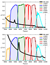 |
Fig. 1. Example of the artificial spectrum of an AGN at z = 0 (upper panel) and high redshift z = 2.7 (lower panel). The LSST filters are overplotted. |
2.3. Construction of a single dense light curve
We first constructed a single dense stochastic light curve. To do this, we used the algorithm developed by Timmer & Koenig (1995). We usually assumed a broken power-law shape for the underlying power spectrum, with two frequency breaks, fb1 and fb2, and three slopes (α1,α2, and α3). This parameterization is more general than the damped random walk that is frequently used to model AGN light curves (Kelly et al. 2009), which would correspond to fb1 = fb2, and α1 = 0, α3 = 2. The random aspect appears when the power spectrum specified in the frequency domain is Fourier-transformed to the time domain because the power spectrum specifies only the value of the Fourier transform, but not the phase. This phase was thus adopted as random, which is justified by studies of AGN light curves. This led to (an almost arbitrary) number of light curves corresponding to the same power spectrum and thus representing the same set of parameters. As advised by Uttley et al. (2005), in the next step the exponent of the constructed stochastic light curve was calculated for final use which allowed us to avoid negative values when the fluctuations were strong, and it additionally reproduced the standard correlation between the rms and flux and the associated log-normal flux distribution seen in accreting sources. The remaining parameters are the time step in the dense light curve, δT, and the total duration of the light curve, T. The normalization of the curve is provided by the assumed total variance. This light curve later represents the continuum band, which is relatively free from contamination by a strong emission line.
2.4. Delayed dense light curve
In the next step, we created a delayed dense light curve. This required the assumption of the time delay expected in a given object. In our modeling, we used the radius-luminosity relation derived as
![Mathematical equation: $$ \begin{aligned} \log {(\tau _{\rm obs} \;[{light-days}])}= \beta + \gamma \log {L_{3000,44}} + \log (1+z), \end{aligned} $$](/articles/aa/full_html/2023/07/aa45844-23/aa45844-23-eq1.gif) (1)
(1)
where L3000, 44 is the monochromatic absolute luminosity at 3000 Å in units of 1044, in erg s−1, τobs is the time delay in the observer’s frame, and z is the source redshift. The values of the coefficients can be taken from the observational studies of the R − L relation9:16 am (e.g., Kaspi et al. 2000; Peterson et al. 2004; Bentz et al. 2013), and they are slightly different for various lines, in particular, the delay for CIV is shorter than the typical delay for Hβ and Mg II (e.g., Lira et al. 2018). This was not included in the simulations. We used the same R − L for all the lines, and the fixed parameters were set as default (β = 1.573, γ = 0.5). The choice of the slope was motivated theoretically by the failed radiatively accelerated dusty outflow (FRADO) model of the BLR (Czerny & Hryniewicz 2011; Czerny et al. 2015, 2017; Naddaf et al. 2021; Naddaf & Czerny 2022), which is well justified for Hβ and Mg II, but not for CIV, which belongs to the high-ionization lines and forms in the dustless line-driven wind, closer to the black hole.
We used the delay given by Eq. (1) to shift the original dense line light curve. Additionally, because the reprocessing in the BLR happens in an extended medium, the original dense curve should be convolved with the response function of the BLR. These response functions were derived observationally for a few nearby sources (e.g., Grier et al. 2013; Xiao et al. 2018; Du et al. 2018a; Horne et al. 2021). Attempts to do this for Mg II are complicated by the presence of the underlying Fe II component (Panda 2021; Prince et al. 2022b). Therefore, in the current paper, we simply assumed the response function in the form of a symmetric Gaussian shape, with the time shift set by Eq. (1), and the width σBLR of 10% of the same delay. We also performed tests using a half-Gaussian shape for this purpose as an exception, as was done in the simulations of the time delay by Jaiswal et al. (2023).
2.5. Cadence in all six photometric bands
As argued, for example, by Malik et al. (2022), general sampling, and in particular, seasonal gaps, is a critical issue for a successful delay recovery. Thus, in order to realistically replicate the actual LSST cadence, we used the operation simulator (OpSim) results provided by the VRO-LSST data management team. For the wide-fast-deep (WFD) MS survey, we used the OpSim run baseline_v2.0_10yrs and extracted the 5σ depth light curves for the six bands (ugrizy), determined for 30-second exposures. We made a random search using a 3.5° × 3.5° search area and limited the sky coordinates (RA, Dec) within 0.01 dispersion. This criterion allowed us to choose roughly the 5σ depth for the same (synthetic) source across the six bands. We made a similar search for the deep-drilling field surveys, where we use the OpSim Run: ddf_v1.7_nodither_10yrs. We used these two cadences in most of our simulations, referring to them as DDF and main survey (MS) for simplicity. The 5σ depth in principle informs us about the photometric accuracy of the measurement, depending on the adopted luminosity and redshift of the source, but this is not yet incorporated in the software, and we used a fixed photometric accuracy. However, the typical limit in the g band in the selected field is 24.5 mag, which corresponds to a 5σ detection of an AGN with log L3000 = 43.814 in erg s−1 (we use values of the luminosity L in units of erg s−1 throughout the paper), according to the online AGN calculator (Kozłowski 2015). This means that a quasar with an adopted log L3000 = 44.7 at redshift 2 will be detected with 0.06 mag error and a quasar at log L3000 = 45.7 will be detected roughly with 0.02 mag error. However, some of the exposures are repeated two to three times within 6 h for the MS and five to ten times in DDF within a very short time period of 5–10 min. While these multiple observations do not sample the AGN variability in practice, they effectively lower the error. As a default, we used an even much lower error to emphasize the problems that are directly caused by the red-noise character of the light curves combined with the planned sampling.
We selected two bands for the time-delay measurement: One band that is strongly contaminated by one of the broad emission lines, and the other band was free of contamination, which closely represents the continuum, and neighbors the selected contaminated band. Since in the future we may wish to also use the photometry from other bands to model the continuum, we currently read all the simulated observational dates from the LSST cadence simulator for a selected specific position on the sky and a specific cadence model. This is currently done externally; the cadence is extracted using the simulated databases from the LSST operation simulator, which are processed locally using PYTHON and SQLITE and stored in the form of an ASCII file.
2.6. Creating two simulated photometric light curves
With two dense light curves representing the continuum and the line emission, as described in Sects. 2.3 and 2.4, as well as simulated dates of the measurements in the two selected bands (Sect. 2.5), we now construct the modeled light curves. They were constructed by adding the reference curve and the delayed curve, but with the delay curve normalized by the level of line contamination, as specified in Sect. 2.2, and by interpolation to the planned cadence. Observations in the two bands are not simultaneous, they simply follow the set LSST cadence for the chosen location in the sky. Only one of the two constructed curves is strongly contaminated by the BLR, as designed, so that it contains the relatively delayed signal, typically of about a few percent, depending on the redshift and adopted strength of the lines.
At this stage, we also included the additional noise due to the expected photometric error (P) in magnitudes, which (for the small error) is equivalent to the dimensionless fractional error. This was done assuming the photometric accuracy in magnitudes and by adding a Poisson noise to the curve by multiplying each data point flux by (1 + PσP), where σP is the random number representing the Gaussian distribution with zero mean and a dispersion of 1.
In this approach, we neglected the time delays between the nearby continuum bands used in the process, which are generated by the reverberation in the accretion disk. This is an approximation made for simplicity because we concentrated on the plausibility of the recovery of the line delays. The intrinsic continuum delays between the continuum bands are much shorter, about one day to a few days, and their modeling involves the assumption of the height of the irradiating source (see, e.g., Kammoun et al. 2021, for the time-delay plots). The measured delays frequently appear to be longer, but this is quite likely a result of the BLR contamination (e.g., Netzer 2022). Sparse monitoring of the main survey should not be affected by intrinsic continuum time delays. DDF monitoring might be used to disentangle the intrinsic accretion disk delays and the BLR, but we do not address this issue in the current paper. It is important to note that the BLR time delays basically scale with the monochromatic luminosity as the square root (see Eq. (1), where γ ∼ 0.5), and the same scaling is expected from the accretion disk reverberation (e.g., Collier et al. 1999; Cackett et al. 2007) so that the intrinsic continuum time delay should always be shorter for all objects. An example of the two dense light curves representing the uncontaminated photometric channel, the convolution representing the contaminated channel, and the observational points representing the actual cadence is shown in Fig. 2.
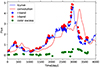 |
Fig. 2. Example of the artificial dense light curve (continuous blue line), its convolution with the BLR response (continuous red line), observational points in i band set by the cadence (red circles), and observational points in r set by the cadence, with contamination from the CIV line (blue circles). Green points represent the net contamination for ϵi = 1.0 (see Eq. (2)). The delay is calculated between the green and blue points. We adopt standard values of the parameters from Table 2 and z = 2.7. |
2.7. First stage of the preparation for the time-delay measurement
We initially tested whether the time delay could be directly measured from the two photometric curves. However, the measurements were very inconclusive because the second light curve contained only a few percent of the delayed line emission. As discussed in previous studies of photometric reverberation mapping (Pozo Nuñez et al. 2012, 2015), the varying AGN continuum must be removed before cross-correlation techniques are used. This can be achieved by subtracting a fraction of the continuum traced by a band with negligible line contribution. To improve the chances of the delay measurement, we therefore first subtracted the relatively uncontaminated curve F1(t) from the contaminated curve, F2(t),
 (2)
(2)
to select ten values of the coefficient, ϵi, equally spaced between 0.85 and 1.15. This required interpolation because F1 and F2 are not measured at the same moment. An example of this subtraction is shown in Fig. 2 with the green points. The time delay is measured for all ten values of ϵi, and the time delay was later set to the value that favored the quality of the time-delay fit.
2.8. Time-delay measurements
Finally, we determined the time delay using one of the two methods. The default method used in the current paper is the χ2 method (for details, see Czerny et al. 2013 and Bao et al. 2022). Optionally, the interpolated cross-correlation function (ICCF) can be used, which is described in detail by Gaskell & Peterson (1987) and Peterson et al. (1998, 2004). We searched for the delay imposing the lower time-delay limit at 0.25 of the assumed delay, and the maximum time delay was determined as the lower of the two values: half of the total duration of the campaign, and 1.9 of the assumed delay. The errors in the delay measurement in both cases were set by the dispersion (i.e., standard deviation) in the delay measurements obtained from 100 statistical realizations of the initial stochastic light curve described in Sect. 2.3.
To measure the time-lags, we also tested the Javelin code (Zu et al. 2011, 2013). We ran numerous tests on the simulated data. The method, when properly applied, takes more time and does not give better results. We discuss this issue in Appendix A.
2.9. Assigning representative parameter values
Since the model has many parameters, we first set the representative parameters that were finally included in Table 2 to show the basic trend more easily. We used the SDSS DR14 QSO catalog (Rakshit et al. 2020) to obtain the distribution of the quasar luminosities, line intensities, and line widths. The parent sample from Rakshit et al. (2020) contains spectroscopically measured parameters such as line and continuum luminosities, line widths and equivalent widths for 526 265 SDSS quasars. We considered the distribution of the relevant parameters that serve as input to our code, that is, the continuum luminosity at 3000 Å (or L3000 Å), the line widths (FWHM) for the prominent broad emission lines (C IV, Mg II, and Hβ), and their equivalent widths (EWs). We also considered the EW for the optical Fe II emission integrated between 4434–4684 Å, which is an important contaminant and coolant in the BLR (Boroson & Green 1992; Verner et al. 1999; Shen & Ho 2014; Marinello et al. 2016; Panda et al. 2018; Marziani et al. 2018; Panda 2022). For the L3000 Å, the DR14 QSO catalog provides a quality flag to assess the goodness of fit in addition to the luminosity and corresponding error for each source. the quality flag = 0 corresponds to a good-quality measurement, while measurements with the quality flag > 0 may not be reliable either due to poor S/N or poor spectral decomposition. We therefore filtered sources with L3000 Å > 0 and a corresponding quality flag = 0. This returned 405 077 sources. The first panel in Fig. 3 shows the distribution of L3000 Å for these sources. We similarly created subsamples for the FWHMs and EWs of the broad emission lines. Their distributions are reported in the other panels of Fig. 3. For the FWHMs and the EWs, there are no quality flags. In addition to filtering for sources with value > 0 (here value represents the FWHM or EW for the emission lines of interest), we therefore employed an additional filter: evalue/value < 0.1 (where evalue represents the errors for the corresponding value). We realized that these original distributions had a tail with absurdly high values of about 4–5 × 10⁵ for the FWHMs and ∼108 for the EWs. To filter these erroneously fitted cases, we further restricted each of our subsamples within an upper limit ≳99th percentile. This upper limit was employed uniquely for each case. The final distributions thus obtained are shown in the remaining panels in Fig. 3. The overall counts in each subsample, the median value, and the respective 16th and 84th percentiles for each distribution are tabulated in Table 3. We note that this final filtering to restrict the upper limits of the subsamples has no noticeable effect on the median 16th and 84th percentiles per distribution. The plots from this catalog are shown in Fig. 3. The two exemplary values of the log L3000 luminosity used later in most simulations roughly correspond to 1σ deviation from the mean, that is, 16% of quasars are expected to be brighter than ∼45.7, and 84% are brighter than ∼44.7.
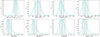 |
Fig. 3. Distribution of the quasar luminosity L3000 Å, line widths (FWHM of C IV, Mg II and Hβ) and equivalent widths (C IV, Mg II, Hβ and optical Fe II) from the DR14 quasar catalog (Rakshit et al. 2020). For each distribution, we show the median (dashed lines) and the 16th and 84th percentiles (dotted lines). These statistics are reported in Table 3 for each of these parameters. |
Model parameters of pairs of photometric light curves.
The line width ∼4000 km s−1 is quite representative for all lines. Line equivalent widths are about 60 Å in the studied sample. We compared this with the distribution of line equivalent widths from the Large Bright Quasar Survey (Forster et al. 2001). This survey reports the EWs of 105 Å for Hβ, 52.7 Å for CIV, and 35.6 Å for the Mg II narrow component, and their broad component most likely (partially or mostly) represents the Fe II contamination. The strength of Hβ is then much higher, and we used a higher value as a default value in our simulations, but we later testes the sensitivity of the results to the adopted parameters.
The representative LSST quasars will not necessarily have the same statistical properties because theLSST will reach considerably deeper (LSST Science Collaboration 2009; Ivezić et al. 2019). In this study, we did not aim at the use of the luminosity function as was done recently by Shen et al. (2020) to make specific predictions.
2.10. Statistical error of the time-delay recovery
The secondary peaks in the histogram are more problematic (see Appendix). We therefore stress that the reported error bars represent the expected error in a single time-delay measurement if no special tests or a preselection of suitable curves is made, and no special methods sensitive to multiple time delays from a single set of data are employed. There are options that can indeed help to decrease the scatter, and we discuss them extensively in the Appendix.
3. Results
3.1. Expectation from the main survey
In this section, we study the prospects of measuring emission line time delays using the data from the main survey, which will cover ten years, but not very densely. We selected the position in the sky. We used the location on the sky centered at (0, −30) for the MS and (9.45, −44.025) for DDF. The sky coordinates (RA, Dec) are reported in degrees.
We followed the steps described in Sect. 2. To illustrate the modeling further, we selected a source with a standard luminosity (see Table 2) located at redshift 2.7. In Fig. 2 we show the two photometric bands, one that is only weakly contaminated (the y band in this case), and the other band, which is strongly contaminated (the r band, in this case, containing the CIV line). We also show the effect of the subtraction described in Sect. 2.2. The two photometric light curves roughly follow each other because the contamination by the delayed line emission is weak, 12% in this case. The direct measurement of the delay between the two bands is therefore not effective, but the subtracted curve follows the delayed curve much better, making the delay measurement much more accurate.
Nevertheless, the cadence in the main survey is not quite suitable for time-delay measurements of relatively faint AGN. The upper panel in Fig. 4 shows that the measured delay is always considerably shorter than the assumed delay because the timescales corresponding to the actual delay are not well probed. However, for brighter sources, the expected time delay is longer, so that the usual sampling characteristic for the main survey is adequate to recover the line delay at least for z > 1 (see the lower panel in Fig. 4). In the actual data analysis, the fainter sources should therefore not be included because the measurement will not be reliable for them. We should also be careful about including the results from too low redshifts, based on Hβ. Although bright quasars, with monochromatic luminosities above log L3000 = 45.7, in erg s−1, are relatively well measured, the expected and recovered time delay at redshifts below 1.0 are still offset.
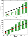 |
Fig. 4. Adopted (black points) and mean recovered (red points) time delay as a function of redshift for faint AGN (log L3000 = 44.7, upper panel) and for bright AGN (log L3000 = 45.7, lower panel) from the main survey. Green error bars are the standard deviation that is expected in a single source measurement, as determined by the use of 100 statistically equivalent simulations. The error of the mean recovered delay is 10% of the dispersion. The other parameters have the standard values given in Table 2. The redshift gaps correspond to no satisfactory selection of the contaminated and uncontaminated bands. |
In our simulations, we adopted the same theoretical time delay for all the lines, even though the CIV line delay is usually shorter. This may cause an additional increase in the error at higher redshifts where the CIV line is used, and in this case, the minimum source luminosity should be even higher. The delay based on Mg II is overall comparable to Hβ (Zajaček et al. 2021) so that the error in our approach is smaller.
3.2. Expectations from the deep drilling fields
In the DDF area, the number of quasars observed is orders of magnitude smaller than expected from the main survey. However, the DDF provide a much denser sampling of the light curve, which increases the quality. This dense coverage importantly allows us to determine some time delays on timescales much shorter than ten years. We thus first discuss the results of the simulations for the entire duration of the project, then for the first two years, and then for the first year of its operation.
In the specific field that we used in the simulations, the number of observing visits is high: 1056 (u), 2239 (g), 4495 (r), 4496 (i), 2330 (z), and 4436 (y). However, at least in this specific field, 6 visits were typically in the minute time separation that for AGN is equivalent to a single visit, although with an improved S/N. When we count only the visits that are separated by one day or more, then the monitoring is limited to 131 (u), 219 (g), 239 (r), 245 (i), 97 (z), and 226 (y) in ten years, and the time separation is frequently of the order of 2 days with long gaps of about a month (except for the six-month seasonal gaps), which averages to a mean separation of 7–9 days in different colors. We illustrate this in Fig. 5, where we plot just the first year of the curve simulated with DDF cadence. Most points are unresolved, and only well-separated point aggregates show up. This is still much better than the main survey, but not as dense as it might seem from the total number of visits. In our simulation, we used all the visits as they are in the cadence. To illustrate this effect on the whole duration of the survey, we show in the lowest two panels of Fig. 5 the histogram of the time separations in the entire ten-year monitoring. We had to use the logarithmic scale for the vertical axis because the time separations that are shorter than 2 days dominate all other separations by some orders of magnitude. We stress that in the actual computations, no binning was performed. We used the data cadence as it was provided.
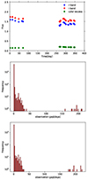 |
Fig. 5. Illustration of the DDF cadence issues. Upper panel: example of the artificial light curve for the first year of observing with DDF cadence in i band (blue circles) and in r band, contaminated by CIV line. Green points represent the net contamination for ϵi = 1.0 (see Eq. (2)). The delay is calculated between the green and the blue points. We adopt standard values of parameters from Table 2, z = 3.276. Middle panel: Histogram of the time separation between the consecutive observation dates in r band in the selected DDF field during the whole ten years. Lower panel: same for the i band. |
The representative results for the whole ten-year monitoring are shown in Fig. 6. For bright quasars, the results from DDF are not considerably better than from the main survey, except for some improvement at the lowest redshifts (below 1.0), where the denser coverage allows a better determination of the time delay (shorter in this case).
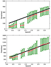 |
Fig. 6. Adopted and recovered time delay as a function of redshift for faint AGN (log L3000 = 44.7, upper panel) and for bright AGN (log L3000 = 45.7, lower panel) from ten years of observations in the DDF. The other parameters have the standard values given in Table 2. |
The difference is highly significant for the faint quasars. They are not reliably sampled in the main survey, but those located in the DDF can be well measured at redshifts above 1.8. This is interesting and important because fainter quasars will dominate the quasar population, so that many faint quasars can be detected in the DDF. In the SDSS (see Fig. 3 and Table 3), about 80% of the quasars are brighter than log L3000 = 44.7, and in the DDF, they would be well measured, while in the main survey, only about 15% of the quasars are bright enough to have delay timescales that are long enough to be measured adequately. The low quality at the lowest redshift is partially related to the large gaps between the seasons. The considerable underestimation of the delay for redshifts between 1.0 and 1.5 arises because the expected/assumed time delay in simulations for the adopted luminosity is about 180 days. At redshifts lower than 0.5, the division of the data into separate seasons may help.
3.3. Expectations from the first year and two years of operation
We first started with a more conservative approach and analyzed the possibility of obtaining interesting results from two years of data. We do not expect any reliable results from the main survey, taking into account the available sampling. However, the cadence of the DDF is much denser, so that time delays of about a year might be measured. In the case of faint AGN, the expected delays are shorter than 400 days, so that the measurement is possible (see Fig. 7, upper panel). The measurements and the predictions are within 1σ error for all redshifts. The mean values are systematically offest from the expected values for all redshifts, however. This offset is caused by data sets that are too short. The measurements are clearly useful for some statistical studies, although a systematic offset of ∼40% should be included. This offset will depend on the exact source luminosity, so that appropriate accompanying simulations would be necessary to improve the quality of the results.
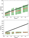 |
Fig. 7. Adopted and recovered time delay as a function of redshift for faint AGN (log L3000 = 44.7, upper panel) and for bright AGN (log L3000 = 45.7, lower panel) from two years of observations in the DDF. The other parameters have the standard values given in Table 2. |
In the case of bright AGN, the expected time delays are so long that only the results for objects at redshifts lower than 0.3 are potentially useful when only two years of data are available. Otherwise, the recovered delay saturates at the maximum allowed by the code, which is set at a minimum between half of the duration of the data set and twice the expected time delay (see Fig. 7, lower panel).
If only the first year of the data is used, the situation is even more difficult. For bright sources, the measurements are unreliable for any redshift, and in the case of faint sources, only the results from low redshifts are promising (see Fig. 8). In any case, AGN at a redshift higher than 0.7 are beyond reach, and conservative searches should rather use an even lower redshift limit of ∼0.4. Nevertheless, it is encouraging overall that some AGN emission-line time delays can be measured from such a short monitoring, with such a highly nonuniform cadence.
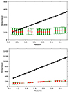 |
Fig. 8. Adopted and recovered time delay as a function of redshift for faint AGN (log L3000 = 44.7, upper panel) and for bright AGN (log L3000 = 45.7, lower panel) from the first year of observations in the DDF. The other parameters have the standard values given in Table 2. |
3.4. Prediction sensitivity of the adopted parameters
Since the number of parameters in our model is large and the representative parameter choice is justified, we tested the dependence of the results only for a selection of assumed parameters. Some of the parameters, such as the FWHM, are of no importance except for a small change in the photometric bands available for time delay measurements.
We tested the dependence on the parameters by mostly concentrating on the first year of the LSST data, since these data will be available relatively soon and can be used to draw important conclusions as soon as possible. However, the trend generally applies to the full ten-year DDF survey as well as to the main survey mode.
We first tested the adopted standard values of the line EWs for the three lines (see Table 2). The assumed standard value for the Hβ line in particular is much higher than the mean value from the SDSS given in Table 3, 150 Å versus 67.36 Å. We therefore recalculated the predictions for all the lines assuming the mean values from Table 3. We considered only the case of the faint AGN population, log L3000 = 44.7. The result is shown in the upper panel of Fig. 9. Comparing the new results to the upper panel in Fig. 8, we see that the change in the EWs of the lines did not affect the results. The delay for redshifts below 0.5 would be well recovered, but higher-redshift sources are beyond the reach of the first year DDF monitoring, even for faint quasars.
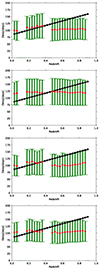 |
Fig. 9. Sensitivity of the simulations to the assumed parameter for the first year of DDF data, faint quasars log L3000 = 44.7. Top panel: alternative values of the line EWs. Second panel: assuming a larger photometric error. Third panel: at shorter timescales for the frequency breaks of the power spectrum. Lowest panel: at lower variability amplitude (see Sect. 3.4 for details). |
We next tested the effect of the assumed photometric accuracy by replacing the rather unrealistic value of 0.001 with 0.02, hence being more conservative. This is clearly much larger than the systematic error, which is expected to be at the level of 0.005 mag (Ivezić et al. 2019). This time, we used the values of the EWs as in the previous plot, and we only changed the expected error. The result (second panel in Fig. 9) is similar to the previous simulations (Fig. 8). The delays are now determined with an error that is larger by up to 20%, but some lo- redshift measurements are still useful.
We also verified whether the adopted high- and low-frequency breaks are important for the simulations. We repeated the computations for the standard accuracy of 0.001, but took the high- and low-frequency breaks to be roughly ten times higher (3.66 × 10⁻⁸ Hz, and 3.66 × 10⁻⁹ Hz, respectively). This caused no systematic effects and a very slight increase in the error by a few percent at most (see Fig. 9). Finally, we tested the adopted level of quasar variability, but in this case, the decrease in the variability level did not affect the results of the simulations (see Fig. 9, lowest panel). Thus the parameterization of the variability does not seem essential for the modeling.
Next, we tested the effect of the assumed R − L relation for the predictions. In our standard simulation setup, we used the same relation for all the lines. In order to determine whether this assumption might be problematic, we performed simulations assuming
 (3)
(3)
for the Hβ line (Khadka et al. 2021),
 (4)
(4)
for the Mg II line (Zajaček et al. 2021), and
 (5)
(5)
for the CIV line (Cao et al. 2022). The difference is most significant for the CIV line, which is suitable for quasars at higher redshifts. In this case, we therefore show the results for bright quasars from the DDF field from the entire ten years of data. This is to be compared with Fig. 6. The new results are shown in Fig. 10. The results at low redshift changed less because they were based on Hβ and Mg II, but a much shorter time delay for CIV created a problem at high redshift. It underpredicted the delay by ∼10%. A considerable problem, however, is seen at the two lowest redshifts, below 0.5. The new formula for the Hβ time delay from Eq. (3) brings values of 142 and 158 days, which are now close to half a year, and the delay determination is strongly affected by the seasonal gap. In our standard simulations, the delay was assumed to be 331 and 360 days for the corresponding two redshifts for bright quasars, so that the problem of the seasonal gap did not appear for this class of sources.
 |
Fig. 10. Sensitivity of the simulations to the assumed parameter for the ten years of DDF data, bright quasars log L3000 = 45.7, in erg s−1, assuming a different radius-luminosity relation for each of the emission lines. Top panel: symmetric Gaussian response. Lower panel: half-Gaussian asymmetric response for the BLR. |
The relations discussed above, representing the time delay as a function of the monochromatic luminosity, are not necessarily universal. There are indications that the time delays are relatively shorter for sources with a high Eddington ratio (e.g., Du et al. 2015, 2016). Knowledge of the Eddington ratio, however, requires knowledge of the black hole mass and the black hole spin. In the case of spectroscopic studies, the problem can be addressed by additionally measuring the black hole mass from the line profiles or by introducing a second parameter into the relation, for example, the normalization of the Fe II pseudo-continuum, which is related to the Eddington ratio (Du et al. 2018b). This is not a good strategy for the sample, however, which is very heterogeneous (Khadka et al. 2022). In the case of photometric measurements, it is not clear how the issue can be addressed in an individual object.
The next potentially important assumption was using a symmetric Gaussian to model the response of the BLR, while in the few cases, when the response function shape was derived from the data, the shape was clearly asymmetric (Horne et al. 2021). For the comparison, we therefore performed simulations with the response function in the form of a half-Gaussian (see, e.g., Jaiswal et al. 2023), but assuming the shift as implied by the formulae and the width as in a standard model, that is, 10% of the time delay. While we did this, we kept the line delays different for each emission line, as in the previous case. We observed that the recovery of the delay in this case is less accurate. The expected values depart by up to ∼20% for the adopted width of the half-Gaussian (see Fig. 10, lower panel). This systematic offset is thus a potential problem, although the recovered and expected time-delay difference is still within 1 σ error.
Finally, we tested other cadences than the two representative ones for MS and DDF. We used the location on the sky (0, −30) for the MS, and for the DDF, we used the ELAIS-S1 centered at (9.45, −44.025), but we tested eight more recently proposed cadences for the MS and for the DDF. We list them in Table 4. In order to make the presentation compact, we plot it by skipping the error bars because they do not change much. We instead show two plots that are color-coded according to the relative difference of the mean time delay, τderived, with the time delay adopted in the simulations, τadopted,
 (6)
(6)
Effective mean separation in the observing dates in r band and the redshift-averaged offset of the mean recovered time delay in comparison to the assumed time delay for bright quasars for ten years of data.
This dimensionless quantity depends strongly on the source luminosity, therefore, we plot it as a function of redshift separately for faint (upper panel of Fig. 11) and bright AGN (lower panel). We used all ten years of the simulated cadence. For most of the cadences, the results are overall similar to those obtained previously. The results for the bright AGN are quite satisfactory, particularly for moderate redshifts. For redshifts z ∼ 0.7, the derived delays are frequently too short. As discussed already by Czerny et al. (2013), for bright quasars, we need five measurements per year if the coverage is uniform and the data is spectroscopic. For a photometric (more difficult) time-delay measurement with nonuniform sampling, we need twice that many data points, and light curves providing less than that cannot be used. For fainter quasars, most of the cadences again underpredict the time delays, which are too short to be properly sampled in the MS mode.
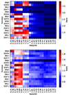 |
Fig. 11. Color-coded relative systematic error of the delay determination for faint (upper panel) and bright (lower panel) AGN in ten years of data for eight MS cadences and eight DDF cadences different from those considered before. The coding scale is different in the lower and upper panels. |
In the case of DDF, the results were qualitatively similar. With the aim to compare them quantitatively, we therefore calculated two global parameters for each cadence. One parameter was the mean separation of visits after treating the observation made within one day as a single exposure. The second parameter was the redshift-averaged value of δ (see Eq. (6)). In Table 4 we list these values for the bright quasars. It is interesting to note that a simple comparison of the number of independent measurements or an actual number of visits is not reflected in the quality. For example, in the cadence S6-DDF, the total number of visits is lower by a factor of 2 than in the remaining cadences (2542, 1672, 2637, and 2209 in g, r, iz bands in comparison with the mean of 5033, 2853, 5132, and 4356, respectively). However, the worst offset occurs for the cadence S3-DDF, which means that the specific distribution of observing dates is important. This offset remains, regardless of the number of observed sources. For accurate results, the offset must therefore be corrected through simulations. The large systematic error for faint sources at redshifts between 1 and 1.5 that is visible in Fig. 6 is seen in all cadences, although it is relatively smaller in S7-DDF.
4. Discussion
The LSST will provide up to ten million quasar detections in the main survey mode and a few thousand higher-quality AGN light curves from the DDF. It will be an enormous leap in the reverberation monitoring of AGN and for the prospects of applying the results to constrain the cosmological models. We thus performed simulations to estimate the prospects of the results from the entire ten-year survey as well as from the first two years and the first year of data collection. A large number of expected time-delay measurements will open an efficient way to study AGN properties, as well as to apply them to cosmology. We should also be aware that the large statistics of the measured time delays may reveal the dependence on the redshift, in addition to the known trends with the Eddington ratio (Du et al. 2018b; Panda 2022; Panda & Marziani 2023). For example, the R − L relation may be affected by a systematic change in the average viewing angle for selected subpopulations of quasars. Currently, we do not see any such trend with the redshift (e.g., Prince et al. 2022a; Dainotti et al. 2022), but the accuracy of this statement is low as the 95% confidence level limit allows a change in the viewing angle from ∼75 deg (at redshift 0) to ∼30 deg (at redshift 3), with a corresponding systematic change in the luminosity distance by a factor of 1.8 (see Fig. 3 in Prince et al. 2022a).
The expected accuracy of the time-delay measurement for a single AGN is about 30% if the source parameters are appropriate for the measurement. During the first year, only the shortest time delays can be measured, which means that only DDF data are useful for this purpose. In addition, only faint AGN at low redshift have a time delay that is short enough to be measured. Using the SDSS AGN statistics for reference, we can expect only 15% of AGN to have redshifts below 0.9, and not all of them are faint. This means that overall, some 10% of the AGN out of about ten thousand located in the DDFs can potentially allow a measurement of the time delay. This is still a few hundred measurements and more than are available at present. It is interesting for statistical studies. For cosmological applications, such a sample will be still too small, particularly because the dispersion in the measurements of line delays is usually high (e.g., Zajaček et al. 2021; Cao et al. 2022, for the most recent cosmological applications). Thus the reduction of the statistical error by a factor of 10 will not lead to high-precision cosmology yet.
Measurements based on two years of data from the DDF will improve the situation considerably, but the critical improvement will come from the whole ten years of data. The DDF data will allow a measurement of time delays for all bright AGN and for most and even faint AGN at a redshift above 1.7. This means that at least half of the quasars in DDFs will have a determined line delay. A thousand measurements will reduce the statistical error by a factor of 30, and it will almost approach an accuracy of 1% in the overall distance determination. An even more spectacular improvement will come from the main survey. Only bright quasars will have delay measurements there, but this means about one million measurements. At face value, this will reduce the statistical error by a factor of 1000, which means a formal subpercent accuracy for cosmological measurements.
However, in this case, the dominant source of the error will be the systematic error. Our simulations show that this systematic error is likely to be present. Our simulations for the ten years of data in the main survey for faint AGN (log L3000 = 44.7) always returns an average time delay that is much shorter than the assumed value (see Fig. 4). The smallest error is for redshifts close to 3, but it is ∼30% smaller than expected. There seem to be no systematic issues with bright objects (log L3000 = 45.7, in erg s−1) between redshift 1.7 and 3.0. A slight deviation appears above 3, and this effect should not be present for somewhat fainter AGN because it is related to time delays that are too long compared with the survey duration. A clear discrepancy is present at the lowest redshift. However, for cosmological applications, it is necessary to cover a broad range of redshifts, including the lowest redshifts. A further study of the systematics present in this case below 1.7 is therefore necessary. The solution may be to use extensive modeling and the appropriate corrections, but they will most likely depend on the specific source luminosity and the actual cadence in the field. Combining the results from the DDF and the main survey will also improve the situation because for DDFs, the results at lower redshifts are more accurate. As mentioned above, the additional intrinsic systematic trends in AGN may also be detected. Separate studies of subclasses of AGN are therefore required. In order to achieve high accuracy of the results, the intrinsic time delays between the continuum bands should also be included in the actual data analysis. The potential errors related to this issue were not estimated in the current study.
The cadence adopted in the simulations is one of the main sources for the offset. We checked that by repeating the computations for the faint quasars, two years of data, assuming the same number of observations as implied by the DDF cadence used in Fig. 7, but assuming a seasonal gap of 180 days between years 1 and 2, and roughly equally spaced observations during the remaining six-month periods. In this case, the agreement between the assumed and recovered time delays is much better, although the dispersion in the redshift recovery is still roughly the same. However, this cadence is not likely to be accepted during the DDF monitoring. Otherwise, we do not see high sensitivity of the line delay recovery on the tested cadences that were considered here. The possibility of measuring the time delay mostly depends on the source luminosity and redshift, and not as much on the actual cadence.
This is clearly different from the measurement of the continuum time delay, where dense sampling is essential, as argued already by Brandt et al. (2018). For this reason, Kovačević et al. (2022) argued that useful measurements can be mad only for DDF, and some of the cadences were favored. Simulations performed by Pozo Nuñez et al. (2023) also request a two- to five-day cadence for continuum delays with the LSST, and such cadence is roughly expected in DDF fields although not forming such a regular pattern as assumed in that paper.
Our simulations are based on the creation of the light curves using the Timmer & Koenig (1995) algorithm. This is not the only method available, although it is fairly general due to a number of parameters entering into the parameterization of the power density spectrum. Other methods of creating artificial light curves are also used, mostly working directly in the time domain, such as the damped random walk (Kelly et al. 2009), the damped harmonic oscillator (Yu et al. 2022), or more complex higher-order CARMA processes (Kelly et al. 2014). These methods were used by Sheng et al. (2022) to simulate quasar light curves in the DDF and aimed at the precise reconstruction of the light curves from the available photometric data. They used the advanced method of stochastic recurrent neural networks and concluded that the recovery precision is most affected by the seasonal gaps. In our simulations, we neglected the narrow components of the emission lines, but for quasars, the narrow components are usually relatively weak.
More importantly, we assumed in the present simulations that we know the luminosity and the redshift of each source. The redshift is important both for the position of the emission lines and also for the luminosity and the estimate of the expected time delay. However, most of the quasars, particularly the fainter sources, will be discovered in the course of the survey, which poses a problem for their identification and the photometric measurement of the redshift. The automatic AGN classifier (see Russeil et al. 2022) is already working in the case of the Zwicky Transient Facility, and a similar classifier is under development for the LSST. The accuracy of the photometric redshifts for AGN is not well established, therefore we did not attempt to model this effect, but it will be likely a considerable source of error in the MS, where spectroscopic follow-up of a large fraction of sources is not realistic. If the photometric errors are small, it would be enough to broaden the redshift ranges, which should be avoided because the band does not contain a full line, which would simply reduce the number of suitable objects.
5. Conclusions
We showed that the recovery of the emission line time delay from the photometric measurements available from the LSST is possible for a significant fraction of the quasars. The expected time delays depend on the source luminosity, but quasars typically range from ∼100 days to over three years, so that the specific cadence requirements are not as critically important as for continuum time delays. We list our results below.
-
For quasars brighter than log L3000 = 45.7, the cadence available in the main survey is in general good enough to allow measurements of the line time delay with respect to the continuum; individual measurement errors are large, about 40%, but in most of the cadences, the systematic offset is 10–15%. Combining measurements for many quasars will therefore allow us to statistically study trends such as the radius-luminosity relation.
-
For quasars fainter than log L3000 = 44.7, the main survey is not recommended, and for the intermediate-luminosity quasars, the redshift limit of practical use will have to be set through simulations.
-
The line time delays in quasars fainter than log L3000 = 44.7 can be successfully measured from the DDF. In this case, even the first two years of data are enough, and the longer data set does not improve the delay measurement at lower redshifts unless the data are sampled in shorter periods or are detrended.
-
Bright quasars can be also studied with dense sampling when they are located in DDF fields, but this only slightly decreases the individual error (down to below ∼30%).
-
Each of the considered cadences leads to some systematic offset between the delay assumed in the setup and the recovered time delay. This offset (about 10%) will remain even if numerous quasars are measured. High-quality results therefore require correcting for this offset by numerical simulations. This offset will depend on quasar properties as well as cadence, photometric errors, and the time-delay measurement method.
-
Some of the considered cadences are better than others, but for the line-delay measurements, the cadence is apparently not a critical issue.
Therefore, with proper selection of the source luminosities and corresponding redshift ranges, we expect reliable measurements of the time delays for a significant fraction of the quasars observed in the main survey mode when the project is completed. The exact fraction could be estimated when the observational cadence is set. Results for intrinsically fainter sources located in DDF fields and with low redshifts can be obtained even from the data collected during the first year of the project.
The results of the OpSim runs are hosted on the publicly available website: http://astro-lsst-01.astro.washington.edu:8080.
Acknowledgments
This project has received funding from the European Research Council (ERC) under the European Union’s Horizon 2020 research and innovation program (grant agreement No. [951549]). The project was partially supported by the Polish Funding Agency National Science Centre, project 2017/26/A/ST9/00756 (MAESTRO 9), project 2018/31/B/ST9/00334 (OPUS 16), and OPUS-LAP/GAR-LA bilateral project (2021/43/I/ST9/01352/OPUS 22 and GF23-04053L). Partial support came from MNiSW grant DIR/WK/2018/12. This project has received funding from the European Research Council (ERC) under the European Union’s Horizon 2020 research and innovation program (grant agreement No. [951549]). SP acknowledges the Conselho Nacional de Desenvolvimento Científico e Tecnológico (CNPq) Fellowships 164753/2020-6 and 300936/2023-0. MZ, RP, and BC acknowledge the Czech-Polish mobility program (MŠMT 8J20PL037 and PPN/BCZ/2019/1/00069). SK acknowledges the National Science Centre grant (OPUS16, 2018/31/B/ST9/00334). A.B.K., D.I., and L.Č.P. acknowledge funding provided by the University of Belgrade-Faculty of Mathematics (contract No. 451-03-47/2023-01/200104) and Astronomical Observatory Belgrade (contract No. 451-03-47/2023-01/200002) through the grants by the Ministry of Science, Technological Development and Innovation of the Republic of Serbia. D.I. acknowledges the support of the Alexander von Humboldt Foundation. M.L. M.-A. acknowledges financial support from Millenium Nucleus NCN19_058 (TITANs). FPN gratefully acknowledges the generous and invaluable support of the Klaus Tschira Foundation. MZ acknowledges the financial support from the GAČR-LA grant no. GF22-04053L.
References
- Bao, D.-W., Brotherton, M. S., Du, P., et al. 2022, ApJS, 262, 14 [NASA ADS] [CrossRef] [Google Scholar]
- Bentz, M. C., & Katz, S. 2015, PASP, 127, 67 [Google Scholar]
- Bentz, M. C., Walsh, J. L., Barth, A. J., et al. 2009, ApJ, 705, 199 [NASA ADS] [CrossRef] [Google Scholar]
- Bentz, M. C., Denney, K. D., Grier, C. J., et al. 2013, ApJ, 767, 149 [Google Scholar]
- Blandford, R. D., & McKee, C. F. 1982, ApJ, 255, 419 [Google Scholar]
- Boroson, T. A., & Green, R. F. 1992, ApJS, 80, 109 [Google Scholar]
- Brandt, W. N., Ni, Q., Yang, G., et al. 2018, arXiv e-prints [arXiv:1811.06542] [Google Scholar]
- Bruhweiler, F., & Verner, E. 2008, ApJ, 675, 83 [NASA ADS] [CrossRef] [Google Scholar]
- Bruzual, G., & Charlot, S. 2003, MNRAS, 344, 1000 [NASA ADS] [CrossRef] [Google Scholar]
- Cackett, E. M., Horne, K., & Winkler, H. 2007, MNRAS, 380, 669 [Google Scholar]
- Cackett, E. M., Bentz, M. C., & Kara, E. 2021, iScience, 24, 102557 [NASA ADS] [CrossRef] [Google Scholar]
- Cao, S., Zajaček, M., Panda, S., et al. 2022, MNRAS, 516, 1721 [NASA ADS] [CrossRef] [Google Scholar]
- Cid Fernandes, R., Mateus, A., Sodré, L., Stasińska, G., & Gomes, J. M. 2005, MNRAS, 358, 363 [Google Scholar]
- Collier, S., Horne, K., Wanders, I., & Peterson, B. M. 1999, MNRAS, 302, L24 [NASA ADS] [CrossRef] [Google Scholar]
- Czerny, B., & Hryniewicz, K. 2011, A&A, 525, L8 [NASA ADS] [CrossRef] [EDP Sciences] [Google Scholar]
- Czerny, B., Hryniewicz, K., Maity, I., et al. 2013, A&A, 556, A97 [NASA ADS] [CrossRef] [EDP Sciences] [Google Scholar]
- Czerny, B., Modzelewska, J., Petrogalli, F., et al. 2015, Adv. Space Res., 55, 1806 [NASA ADS] [CrossRef] [Google Scholar]
- Czerny, B., Li, Y.-R., Hryniewicz, K., et al. 2017, ApJ, 846, 154 [NASA ADS] [CrossRef] [Google Scholar]
- Czerny, B., Olejak, A., Rałowski, M., et al. 2019, ApJ, 880, 46 [Google Scholar]
- Czerny, B., Martínez-Aldama, M. L., Wojtkowska, G., et al. 2021, Acta Physica Polonica A, 139, 389 [NASA ADS] [CrossRef] [Google Scholar]
- Dainotti, M. G., Bargiacchi, G., Lenart, A. Ł., et al. 2022, ApJ, 931, 106 [NASA ADS] [CrossRef] [Google Scholar]
- Du, P., Hu, C., Lu, K.-X., et al. 2015, ApJ, 806, 22 [NASA ADS] [CrossRef] [Google Scholar]
- Du, P., Lu, K.-X., Zhang, Z.-X., et al. 2016, ApJ, 825, 126 [CrossRef] [Google Scholar]
- Du, P., Zhang, Z.-X., Wang, K., et al. 2018a, ApJ, 856, 6 [NASA ADS] [CrossRef] [Google Scholar]
- Du, P., Brotherton, M. S., Wang, K., et al. 2018b, ApJ, 869, 142 [CrossRef] [Google Scholar]
- Forster, K., Green, P. J., Aldcroft, T. L., et al. 2001, ApJS, 134, 35 [NASA ADS] [CrossRef] [Google Scholar]
- Gaskell, C. M., & Peterson, B. M. 1987, ApJS, 65, 1 [NASA ADS] [CrossRef] [Google Scholar]
- GRAVITY Collaboration (Sturm, E., et al.) 2018, Nature, 563, 657 [Google Scholar]
- GRAVITY Collaboration (Amorim, A., et al.) 2020, A&A, 643, A154 [NASA ADS] [CrossRef] [EDP Sciences] [Google Scholar]
- GRAVITY Collaboration (Amorim, A., et al.) 2021, A&A, 654, A85 [NASA ADS] [CrossRef] [EDP Sciences] [Google Scholar]
- Grier, C. J., Peterson, B. M., Horne, K., et al. 2013, ApJ, 764, 47 [NASA ADS] [CrossRef] [Google Scholar]
- Grier, C. J., Trump, J. R., Shen, Y., et al. 2017, ApJ, 851, 21 [NASA ADS] [CrossRef] [Google Scholar]
- Haas, M., Chini, R., Ramolla, M., et al. 2011, A&A, 535, A73 [NASA ADS] [CrossRef] [EDP Sciences] [Google Scholar]
- Homayouni, Y., Trump, J. R., Grier, C. J., et al. 2020, ApJ, 901, 55 [Google Scholar]
- Horne, K., De Rosa, G., Peterson, B. M., et al. 2021, ApJ, 907, 76 [Google Scholar]
- Hryniewicz, K., Czerny, B., Pych, W., et al. 2014, A&A, 562, A34 [NASA ADS] [CrossRef] [EDP Sciences] [Google Scholar]
- Ivezić, Ž., Kahn, S. M., Tyson, J. A., et al. 2019, ApJ, 873, 111 [Google Scholar]
- Jaiswal, V. K., Prince, R., Panda, S., & Czerny, B. 2023, A&A, 670, A147 [NASA ADS] [CrossRef] [EDP Sciences] [Google Scholar]
- Kammoun, E. S., Dovčiak, M., Papadakis, I. E., Caballero-García, M. D., & Karas, V. 2021, ApJ, 907, 20 [NASA ADS] [CrossRef] [Google Scholar]
- Kaspi, S., Smith, P. S., Netzer, H., et al. 2000, ApJ, 533, 631 [Google Scholar]
- Kaspi, S., Brandt, W. N., Maoz, D., et al. 2021, ApJ, 915, 129 [NASA ADS] [CrossRef] [Google Scholar]
- Kelly, B. C., Bechtold, J., & Siemiginowska, A. 2009, ApJ, 698, 895 [Google Scholar]
- Kelly, B. C., Becker, A. C., Sobolewska, M., Siemiginowska, A., & Uttley, P. 2014, ApJ, 788, 33 [NASA ADS] [CrossRef] [Google Scholar]
- Khadka, N., Yu, Z., Zajaček, M., et al. 2021, MNRAS, 508, 4722 [NASA ADS] [CrossRef] [Google Scholar]
- Khadka, N., Martínez-Aldama, M. L., Zajaček, M., Czerny, B., & Ratra, B. 2022, MNRAS, 513, 1985 [NASA ADS] [CrossRef] [Google Scholar]
- Khadka, N., Zajaček, M., Prince, R., et al. 2023, MNRAS, 522, 1247 [NASA ADS] [CrossRef] [Google Scholar]
- Kovačević, A. B., Ilić, D., Popović, L. Č., et al. 2021, MNRAS, 505, 5012 [CrossRef] [Google Scholar]
- Kovačević, A. B., Radović, V., Ilić, D., et al. 2022, ApJS, 262, 49 [CrossRef] [Google Scholar]
- Kozłowski, S. 2015, Acta Astron., 65, 251 [NASA ADS] [Google Scholar]
- Krolik, J. H. 1999, Active Galactic Nuclei: From the Central Black Hole to the Galactic Environment (Princeton, N.J: Princeton University Press) [Google Scholar]
- Lira, P., Kaspi, S., Netzer, H., et al. 2018, ApJ, 865, 56 [NASA ADS] [CrossRef] [Google Scholar]
- LSST Science Collaboration (Abell, P. A., et al.) 2009, arXiv e-prints [arXiv:0912.0201] [Google Scholar]
- Lu, K.-X., Du, P., Hu, C., et al. 2016, ApJ, 827, 118 [CrossRef] [Google Scholar]
- Malik, U., Sharp, R., Martini, P., et al. 2022, MNRAS, 516, 3238 [NASA ADS] [CrossRef] [Google Scholar]
- Maoz, D., Netzer, H., Leibowitz, E., et al. 1990, ApJ, 351, 75 [NASA ADS] [CrossRef] [Google Scholar]
- Marinello, M., Rodríguez-Ardila, A., Garcia-Rissmann, A., Sigut, T. A. A., & Pradhan, A. K. 2016, ApJ, 820, 116 [Google Scholar]
- Martínez-Aldama, M. L., Czerny, B., Kawka, D., et al. 2019, ApJ, 883, 170 [CrossRef] [Google Scholar]
- Marziani, P., Dultzin, D., Sulentic, J. W., et al. 2018, Front. Astron. Space Sci., 5, 6 [CrossRef] [Google Scholar]
- Naddaf, M. H., & Czerny, B. 2022, A&A, 663, A77 [NASA ADS] [CrossRef] [EDP Sciences] [Google Scholar]
- Naddaf, M.-H., Czerny, B., & Szczerba, R. 2021, ApJ, 920, 30 [NASA ADS] [CrossRef] [Google Scholar]
- Netzer, H. 2022, MNRAS, 509, 2637 [NASA ADS] [Google Scholar]
- Netzer, H., & Maoz, D. 1990, ApJ, 365, L5 [NASA ADS] [CrossRef] [Google Scholar]
- Panda, S. 2021, PhD Thesis, Polish Academy of Sciences, Instituteof Physics [Google Scholar]
- Panda, S. 2022, Front. Astron. Space Sci., 9, 409 [NASA ADS] [CrossRef] [Google Scholar]
- Panda, S., & Marziani, P. 2023, Front. Astron. Space Sci., 10, 1130103 [NASA ADS] [CrossRef] [Google Scholar]
- Panda, S., Czerny, B., Adhikari, T. P., et al. 2018, ApJ, 866, 115 [CrossRef] [Google Scholar]
- Panda, S., Martínez-Aldama, M. L., & Zajaček, M. 2019, Front. Astron. Space Sci., 6, 75 [NASA ADS] [CrossRef] [Google Scholar]
- Peterson, B. M. 1993, PASP, 105, 247 [NASA ADS] [CrossRef] [Google Scholar]
- Peterson, B. M., & Gaskell, C. M. 1991, ApJ, 368, 152 [NASA ADS] [CrossRef] [Google Scholar]
- Peterson, B. M., Balonek, T. J., Barker, E. S., et al. 1991, ApJ, 368, 119 [NASA ADS] [CrossRef] [Google Scholar]
- Peterson, B. M., Wanders, I., Horne, K., et al. 1998, PASP, 110, 660 [Google Scholar]
- Peterson, B. M., Berlind, P., Bertram, R., et al. 2002, ApJ, 581, 197 [NASA ADS] [CrossRef] [Google Scholar]
- Peterson, B. M., Ferrarese, L., Gilbert, K. M., et al. 2004, ApJ, 613, 682 [Google Scholar]
- Pozo Nuñez, F., Ramolla, M., Westhues, C., et al. 2012, A&A, 545, A84 [NASA ADS] [CrossRef] [EDP Sciences] [Google Scholar]
- Pozo Nuñez, F., Haas, M., Ramolla, M., et al. 2014, A&A, 568, A36 [NASA ADS] [CrossRef] [EDP Sciences] [Google Scholar]
- Pozo Nuñez, F., Ramolla, M., Westhues, C., et al. 2015, A&A, 576, A73 [NASA ADS] [CrossRef] [EDP Sciences] [Google Scholar]
- Pozo Nuñez, F., Bruckmann, C., Deesamutara, S., et al. 2023, MNRAS, 522, 2002 [CrossRef] [Google Scholar]
- Prince, R., Hryniewicz, K., Panda, S., Czerny, B., & Pollo, A. 2022a, ApJ, 925, 215 [NASA ADS] [CrossRef] [Google Scholar]
- Prince, R., Zajaček, M., Czerny, B., et al. 2022b, A&A, 667, A42 [NASA ADS] [CrossRef] [EDP Sciences] [Google Scholar]
- Prince, R., Zajaček, M., Panda, S., et al. 2023, A&A, submitted, [arXiv:2304.13763] [Google Scholar]
- Rakshit, S., Stalin, C. S., & Kotilainen, J. 2020, ApJS, 249, 17 [Google Scholar]
- Russeil, E., Ishida, E. E. O., Le Montagner, R., Peloton, J., & Moller, A. 2022, arXiv e-prints [arXiv:2211.10987] [Google Scholar]
- Shen, Y., & Ho, L. C. 2014, Nature, 513, 210 [NASA ADS] [CrossRef] [Google Scholar]
- Shen, Y., Horne, K., Grier, C. J., et al. 2016, ApJ, 818, 30 [NASA ADS] [CrossRef] [Google Scholar]
- Shen, X., Hopkins, P. F., Faucher-Giguère, C.-A., et al. 2020, MNRAS, 495, 3252 [Google Scholar]
- Sheng, X., Ross, N., & Nicholl, M. 2022, MNRAS, 512, 5580 [CrossRef] [Google Scholar]
- Śniegowska, M., Czerny, B., You, B., et al. 2018, A&A, 613, A38 [NASA ADS] [CrossRef] [EDP Sciences] [Google Scholar]
- Timmer, J., & Koenig, M. 1995, A&A, 300, 707 [NASA ADS] [Google Scholar]
- Uttley, P., McHardy, I. M., & Vaughan, S. 2005, MNRAS, 359, 345 [NASA ADS] [CrossRef] [Google Scholar]
- Verner, E. M., Verner, D. A., Korista, K. T., et al. 1999, ApJS, 120, 101 [NASA ADS] [CrossRef] [Google Scholar]
- Watson, D., Denney, K. D., Vestergaard, M., & Davis, T. M. 2011, ApJ, 740, L49 [CrossRef] [Google Scholar]
- Xiao, M., Du, P., Lu, K.-K., et al. 2018, ApJ, 865, L8 [NASA ADS] [CrossRef] [Google Scholar]
- Yu, Z., Martini, P., Davis, T. M., et al. 2020, ApJS, 246, 16 [Google Scholar]
- Yu, W., Richards, G. T., Vogeley, M. S., Moreno, J., & Graham, M. J. 2022, ApJ, 936, 132 [NASA ADS] [CrossRef] [Google Scholar]
- Zajaček, M., Czerny, B., Martinez-Aldama, M. L., et al. 2020, ApJ, 896, 146 [Google Scholar]
- Zajaček, M., Czerny, B., Martinez-Aldama, M. L., et al. 2021, ApJ, 912, 10 [CrossRef] [Google Scholar]
- Zu, Y., Kochanek, C. S., & Peterson, B. M. 2011, ApJ, 735, 80 [NASA ADS] [CrossRef] [Google Scholar]
- Zu, Y., Kochanek, C. S., Kozłowski, S., & Udalski, A. 2013, ApJ, 765, 106 [NASA ADS] [CrossRef] [Google Scholar]
Appendix A: Error of the delay measurement in simulations
A.1. Exemplary histograms of the time delay
As outlined in Section 2.10, we used 100 random realizations of the process to determine the time-delay accuracy. The mean time delay is determined as the average of the 100 delays, and the error as the dispersion. This is a very simple procedure, but a more advanced procedure seems to be problematic because the time delay of the BLR lines measured from the photometry is difficult.
We illustrate the distribution of the 100 time delays in Figure A.1. The computations were made for the standard model, sain Survey cadence, redshift z = 1.93, and a quasar luminosity of log L3000 = 45.7, L3000 in erg s−1. The delays do not have a Gaussian distribution. Instead, a few peaks are visible. The mean of the derived time delays for the adopted parameters is 778.57 days, while the maximum in the histogram is at 768.12 days in the observed frame. The dispersion calculated from the delays gives 361.99 days, which would imply the results for the time delay with 1 σ error between 416.58 days and 1140.56 days. When we determine the 1 sigma error from the actual complex histogram, the corresponding numbers are 241.87 days and 1131.30 days. The error is therefore somewhat larger due to the complex shape. However, the representative values can be derived from our simplified approach.
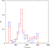 |
Fig. A.1. Example of the histogram of the 100 random realizations for the time delay (blue histogram), and 1000 realizations of the same process (red histogram). The assumed redshift is 1.93, and the assumed luminosity is log L3000 = 45.7, L3000 in erg s−1,. The expected time delay is 776.27 days. |
We repeated the same simulation, but using 1000 realizations instead of 100. The results are also plotted in Figure A.1. In this case, we obtain the mean delay of 799.58 days, with a dispersion of 340.19 days. The expected dispersion is large. The 1 sigma result is between 427.96 days and 1174.56 days when it is determined from the histogram. A larger number of statistical realizations does not change the histogram essentially. A secondary peak again appears at the shortest delays as well as at the longest delays, but the central peak is close to the expected value.
The histogram has additional peaks at the highest and the longest delays because the search is performed in a limited range of likely delays. If no range in the search is imposed, the best delay value frequently peaks at zero delays or at the longest wavelengths. The current version of the code for each light-curve set selects only the single best value for the delay. A more advanced version should store three (or more) values and then select the most likely value a posteriori. This certainly should be done when analysing actual data.
A.2. Multiple characters of the best-fit solutions
As mentioned in Section A.1, the best-fit solutions peak at the minimum and the maximum allowed value of the delay during the period search. This is related to the complex character of the function that implies the best fit. In the case of the χ2 method, the best fit corresponds to the minimum value, and the function frequently has a number of minima. We took three of the special solutions shown in Figure A.1 selected in such a way that one has the minimum roughly where expected, while the other two have the minimum at the shortest and the longest delays, respectively. We plot the χ2 distribution for these three cases in Figure A.2.
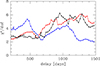 |
Fig. A.2. χ2 distribution as the function of the assumed time delay for three exemplary light curves showing the best-fit time delay of 533 days (black line), 1475 days (maximum allowed; blue line), and 194 days (minimum allowed, red line). They all show a minimum around ∼700 days, but this is only a local minimum. The assumed time delay is 776.27 days. |
Assuming a narrower search range for the delay can automatically reduce the error, but in the case of the actual single datum for a quasar, we will have only a crude estimate of the expected time delay from its redshift and magnitude. The luminosity estimate may additionally be biased by the intrinsic extinction in the source. We thus tested whether confirming the correlation between the two cross-correlated curves helps to eliminate sources that likely lead to the deepest minimum at the wrong location.
A.3. Curve quality and optional curve preselection
We used the 1000 simulated realizations shown in Figure A.1 in order to assess the quality of the quasar curves in the MS. After optimized band subtraction as explained in Eq. 2, we calculated for each of the created pairs of curves the correlation coefficient r with the aim to determine whether a pair preselection can improve the accuracy of the delay determination for most quasars without the loss of many sources. In Figure A.3 we show the number of pairs that is left as a function of the choice of minimum acceptable value of r. Less than 10% of quasars (for the adopted luminosity, redshift, and MS observational pattern) may in principle guarantee reliable measurements. Overall, the curve quality is low, but our simulations most likely represent the actual data quality well. Still, having a million objects or more, we can have encouraging statistics if the results are not biased.
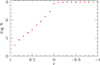 |
Fig. A.3. Number of curve pairs left out of 1000 simulated pairs as a function of the adopted cutoff for the correlation coefficient r. Only 84 pairs out of 1000 have r > 0.3. |
However, selecting realizations (sources) only according to their correlation coefficient does not lead to the successful removal of the wings seen in Figure A.1. In Figure A.4 we show all the values of the 1000 correlation coefficients as a function of the time delay predicted for the given pair. Many of the highest values populate the region in which the time delays are too short. This is expected. Part of the effect is due to the imperfect subtraction of the bands with and without an emission line, which is well modeled in our software. This will be surely present in the actual LSST data. The other aspect may be related to the red-noise character of the quasar light curves. We observed strong local minima for unexpectedly short time delays in our observational spectroscopic studies of the quasar time delay with the Southern African Large Telescope, where the cadence was similar to what is expected from the LSST (Czerny et al. 2019; Zajaček et al. 2020, 2021; Prince et al. 2022b, 2023).
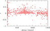 |
Fig. A.4. Values of the correlation coefficients r for 1000 pairs as functions of the measured time delay. High values of r are not only close to the expected time delay, but lie mostly around the lower limit adopted for time-delay measurements. |
Therefore, we performed a combined study of the selection based both on the value of r and the lower limit for the time delay. In the minima of the histogram A.1, we selected the minimum and the maximum time delays as 0.5 Tassumed and 1.5 Tassumed, respectively, and we repeated the previous study. The error bars are clearly smaller for any constraints on the minimum value of r, and they are particularly reduced for r > 0.7, down to 75 days, but only four objects satisfy the two criteria of 1000 simulated pairs. For a conservative choice of r > 0.3, the mean value and the dispersion is 748 ± 146 days, and we have 50 such pairs. The overall trend with the change in the limiting value of r is shown in Figure A.5. We also considered a recalculation of the time delays assuming the same lower and upper limit for a delay search in the code itself, instead of selecting suitable pairs a posteriori. However, running a new set of 1000 simulations with the imposed narrower search for the delay did not improve the situation much. For a conservative case of r > 0.3, the mean value of the dispersion is 681 ± 170 days, and 73 such pairs satisfy this constraint. By selecting 50 out of 1000 cases, we thus reduce the dispersion by a factor of 2.3 (from 340 down to 146 days), but if we were to create 50 bins from the original 1000 objects, then the dispersion would decrease by a factor  . Overall, it therefore seems a better strategy to use all the data and finally bin them. At some level, the systematic effects might become essential, as indicated by the differences between the mean values from the simulations and the assumed values in the simulations, as presented in the figures in Section 3.
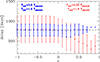 |
Fig. A.5. Time delay from the subsample of 1000 simulations selected according to the minimum value of r (simulations with the maximum value of the correlation coefficient smaller than r were removed from the sample) and the adopted limits for time delay. Narrower limits clearly give smaller errors, which is reflected in the dispersion. |
A.4. Grouping quasars in the actual data
The errors in a single measurement shown in Figures 4 - 10 are large, but a preselection of the sources (except for selecting only a suitable range of redshifts and source luminosity, which does not give an offset between the assumed and the mean recovered value of the time delay) does not seem to give an efficient way to reduce the error. However, if the aim is not an individual source, but the construction of radius-luminosity relation or luminosity distance measurements, the efficient way is to group the measurements.
In the case of the MS survey, we will have at our disposal about one million objects with measured emission line delays. These measurements can be grouped into relatively narrow redshift bins as well as into luminosity bins and then averaged. This should provide an efficient way to reduce the error when establishing a mean trend.
In the case of DDF fields, there is an additional interesting option for fainter sources at low redshift. Since we showed in Figure 8 that for sources like this, one year of data is enough to perform the measurements, the delay can be measured in ten consecutive years independently after the survey is completed, and can then be combined into a single time delay, with additional quality control from the measurement dispersion. This quality control will be essential because we know well that some nearby sources can show large variations in the measured Hβ line delay between the consecutive years, with more complex scaling with luminosity than in statistical samples of different sources (e.g., Peterson et al. 2002; Lu et al. 2016; Horne et al. 2021, for NGC 5548).
A.5. Time-delay measurements using Javelin
We also tested the use of the Javelin code to determine the time delay (Zu et al. 2011, 2013). We focused on the simulations for the MS for bright quasars. When the expected time delay was allowed to be between 0 and 3000 days for all the redshifts, the measured time delay was uncorrelated with the assumed time delay, and no clear trend with the redshift was seen, in contrast to expectations (the assumed rest-frame time delay was redshift independent, but the curves are analyzed in the observed frame). Next, we applied the same restrictions for the time-delay search as in the χ2 method. The minimum value was adopted as 0.25 of the assumed delay in the observed frame, and the maximum value was determined as the smaller value of the two: (a) half of the monitoring period, and (b) 1.9 times the expected time delay. For each redshift we performed 10 statistically independent simulations, i.e., we used ten different (but statistically equivalent) curves created with the Timmer & Koenig (1995) algorithm.
We compared in detail the results for the redshift z = 0.25 and the redshift z = 3.27. For the smaller redshift, we obtained the mean delay from 10 realizations: 285.9 days, the mean error reported by Javelin is 82.1 days (calculated by averaging all reported positive and negative time delays), and the mean dispersion between the best fit time delays is 149.1 days. The dispersion between different realizations of statistically identical curves was larger than the error typically reported by Javelin. For the redshift z = 3.27, the values are the following: mean delay = 1211.6 days, mean error = 160.5 days, and mean dispersion = 179.8 days. In this case, the mean error and the mean dispersion are similar. The mean time delays for z = 0.25 in both Javelin and the χ2 methods are shorter than assumed in the modeling, but within the error (285.9 days and 218.1 days, respectively, vs. 331.0 days assumed in the simulations). For the high redshift z = 3.27, the recovered mean time delays (Javelin: 1211.6 days, and χ2: 1041.8 vs. the assumed value of 1132.4 days) were also consistent with the assumed values. Javelin, except for some underestimation of the error, is also a viable method, but much more computationally intensive.
Appendix B: Details for the cadence simulations
A brief description for each of the selected cadence simulations used in this paper is summarized in Table B.1. For more details, we refer to the official RUBIN_SIM webpage2.
Details of the cadence simulations from the rubin_sim
All Tables
Effective mean separation in the observing dates in r band and the redshift-averaged offset of the mean recovered time delay in comparison to the assumed time delay for bright quasars for ten years of data.
All Figures
|
Fig. 1. Example of the artificial spectrum of an AGN at z = 0 (upper panel) and high redshift z = 2.7 (lower panel). The LSST filters are overplotted. |
| In the text | |
|
Fig. 2. Example of the artificial dense light curve (continuous blue line), its convolution with the BLR response (continuous red line), observational points in i band set by the cadence (red circles), and observational points in r set by the cadence, with contamination from the CIV line (blue circles). Green points represent the net contamination for ϵi = 1.0 (see Eq. (2)). The delay is calculated between the green and blue points. We adopt standard values of the parameters from Table 2 and z = 2.7. |
| In the text | |
|
Fig. 3. Distribution of the quasar luminosity L3000 Å, line widths (FWHM of C IV, Mg II and Hβ) and equivalent widths (C IV, Mg II, Hβ and optical Fe II) from the DR14 quasar catalog (Rakshit et al. 2020). For each distribution, we show the median (dashed lines) and the 16th and 84th percentiles (dotted lines). These statistics are reported in Table 3 for each of these parameters. |
| In the text | |
|
Fig. 4. Adopted (black points) and mean recovered (red points) time delay as a function of redshift for faint AGN (log L3000 = 44.7, upper panel) and for bright AGN (log L3000 = 45.7, lower panel) from the main survey. Green error bars are the standard deviation that is expected in a single source measurement, as determined by the use of 100 statistically equivalent simulations. The error of the mean recovered delay is 10% of the dispersion. The other parameters have the standard values given in Table 2. The redshift gaps correspond to no satisfactory selection of the contaminated and uncontaminated bands. |
| In the text | |
|
Fig. 5. Illustration of the DDF cadence issues. Upper panel: example of the artificial light curve for the first year of observing with DDF cadence in i band (blue circles) and in r band, contaminated by CIV line. Green points represent the net contamination for ϵi = 1.0 (see Eq. (2)). The delay is calculated between the green and the blue points. We adopt standard values of parameters from Table 2, z = 3.276. Middle panel: Histogram of the time separation between the consecutive observation dates in r band in the selected DDF field during the whole ten years. Lower panel: same for the i band. |
| In the text | |
|
Fig. 6. Adopted and recovered time delay as a function of redshift for faint AGN (log L3000 = 44.7, upper panel) and for bright AGN (log L3000 = 45.7, lower panel) from ten years of observations in the DDF. The other parameters have the standard values given in Table 2. |
| In the text | |
|
Fig. 7. Adopted and recovered time delay as a function of redshift for faint AGN (log L3000 = 44.7, upper panel) and for bright AGN (log L3000 = 45.7, lower panel) from two years of observations in the DDF. The other parameters have the standard values given in Table 2. |
| In the text | |
|
Fig. 8. Adopted and recovered time delay as a function of redshift for faint AGN (log L3000 = 44.7, upper panel) and for bright AGN (log L3000 = 45.7, lower panel) from the first year of observations in the DDF. The other parameters have the standard values given in Table 2. |
| In the text | |
|
Fig. 9. Sensitivity of the simulations to the assumed parameter for the first year of DDF data, faint quasars log L3000 = 44.7. Top panel: alternative values of the line EWs. Second panel: assuming a larger photometric error. Third panel: at shorter timescales for the frequency breaks of the power spectrum. Lowest panel: at lower variability amplitude (see Sect. 3.4 for details). |
| In the text | |
|
Fig. 10. Sensitivity of the simulations to the assumed parameter for the ten years of DDF data, bright quasars log L3000 = 45.7, in erg s−1, assuming a different radius-luminosity relation for each of the emission lines. Top panel: symmetric Gaussian response. Lower panel: half-Gaussian asymmetric response for the BLR. |
| In the text | |
|
Fig. 11. Color-coded relative systematic error of the delay determination for faint (upper panel) and bright (lower panel) AGN in ten years of data for eight MS cadences and eight DDF cadences different from those considered before. The coding scale is different in the lower and upper panels. |
| In the text | |
|
Fig. A.1. Example of the histogram of the 100 random realizations for the time delay (blue histogram), and 1000 realizations of the same process (red histogram). The assumed redshift is 1.93, and the assumed luminosity is log L3000 = 45.7, L3000 in erg s−1,. The expected time delay is 776.27 days. |
| In the text | |
|
Fig. A.2. χ2 distribution as the function of the assumed time delay for three exemplary light curves showing the best-fit time delay of 533 days (black line), 1475 days (maximum allowed; blue line), and 194 days (minimum allowed, red line). They all show a minimum around ∼700 days, but this is only a local minimum. The assumed time delay is 776.27 days. |
| In the text | |
|
Fig. A.3. Number of curve pairs left out of 1000 simulated pairs as a function of the adopted cutoff for the correlation coefficient r. Only 84 pairs out of 1000 have r > 0.3. |
| In the text | |
|
Fig. A.4. Values of the correlation coefficients r for 1000 pairs as functions of the measured time delay. High values of r are not only close to the expected time delay, but lie mostly around the lower limit adopted for time-delay measurements. |
| In the text | |
|
Fig. A.5. Time delay from the subsample of 1000 simulations selected according to the minimum value of r (simulations with the maximum value of the correlation coefficient smaller than r were removed from the sample) and the adopted limits for time delay. Narrower limits clearly give smaller errors, which is reflected in the dispersion. |
| In the text | |
Current usage metrics show cumulative count of Article Views (full-text article views including HTML views, PDF and ePub downloads, according to the available data) and Abstracts Views on Vision4Press platform.
Data correspond to usage on the plateform after 2015. The current usage metrics is available 48-96 hours after online publication and is updated daily on week days.
Initial download of the metrics may take a while.